Development of the morphodynamics on Little Ice Age lateral moraines in 10 glacier forefields of the Eastern Alps since the 1950s

Since the end of the Little Ice Age (LIA) in the middle of the 19th century, Alpine glaciers have been subject to severe recession that is enhanced by the recent global warming. The melting glaciers expose large areas with loose sediments in the form of lateral moraines, amongst other forms. Due to their instability and high slope angle, the lateral moraines are reworked by geomorphological processes such as debris flows, slides, or fluvial erosion. In this study, the development of the morphodynamics and changes in geomorphological processes on lateral moraines were observed over decades, based on a selection of 10 glacier forefields in the Eastern Alps. To identify geomorphological changes over time, several datasets of archival aerial images reaching back to the 1950s were utilized in order to generate digital elevation models (DEMs) and DEMs of difference. The aerial images were complemented by recent drone images for selected moraine sections, enabling a high-resolution analysis of the processes currently occurring. The results concerning the development of morphodynamics on lateral moraine sections are diverse: some slopes display a stagnation of the erosion rates, whereas the rates of one section increase significantly; however, the majority of the slopes show a decline in morphodynamics over decades but stay on a high level in many cases. In particular, moraine sections with high morphodynamics at the beginning of the observation period mostly show high erosion rates up until present-day measurements, with values up to 11 cm yr⁻¹. These moraine sections also feature heavy gullying on their upper slopes. A correlation between the development of morphodynamics and the time since deglaciation could scarcely be established. In fact, the results instead indicate that characteristics of the lateral moraines such as the initial slope angle at the time of deglaciation have a significant influence on the later morphodynamics. These observations raise concerns as to whether the until now often conducted analyses based on the comparison of lateral moraine sections with different distances to the glacier terminus, assumed to represent varying time spans since deglaciation, can provide sound evidence concerning the process of stabilization.

1 Introduction

Hambrey (1994, p. 142) wrote that “lateral moraines are among the most impressive features of contemporary glacial mountain environments […], especially above and down stream of those glaciers in the Alps, Scandinavia, the Western Cordillera of North America, and elsewhere […]”. These lateral moraines, often showing a perfect, well-preserved shape (Mortara and Chiarle, 2005), are exposed as a consequence of the extensive glacier melting since the end of the Little Ice Age (LIA, ca. 1450–1850 CE) (Haeberli and Beniston, 1998; Zemp et al., 2008).

The mostly unvegetated and often steep proximal moraine slopes are prone to a variety of geomorphic processes (Curry et al., 2006, 2009; Micheletti et al., 2015b; Chiarle et al., 2007). Water- and gravity-driven processes are occurring on the moraines. These include linear processes such as fluvial rill erosion and debris flows, denudation by slope wash, small mass movements, or sheet erosion by snow gliding (cf. Ballantyne, 2002b; Chiarle et al., 2007; Heckmann et al., 2012; Mortara and Chiarle, 2005; Wetzel, 1992). Debris flows were identified in several studies as the dominant agent of erosion and transport on recently deglaciated sediment-mantled slopes with high slope gradients (Ballantyne, 2002b; Curry et al., 2006). On some of these steep lateral moraines, the geomorphic processes, mainly fluvial processes and in the following also debris flows (cf. Ballantyne and Benn, 1996), lead to the formation of deeply incised gullies (Curry, 1999; Curry et al., 2006). On the other hand, Lukas et al. (2012) point out the unusually high stability and steepness of some lateral moraines in the Alps due to over-consolidation.

Church and Ryder (1972) and Ballantyne (2002a) developed models predicting the course of the erosion rates in a paraglacial landscape and the duration until stabilization. In these models, “paraglacial” refers to a time period in which non-glacial geomorphic processes lead to an adjustment of bedrock and sedimentary landforms after deglaciation; the term also implies that the activity and dynamics of these processes are directly conditioned by deglaciation (Ballantyne, 2002a, b, Benn and Evans, 2010; Church and Ryder, 1972). Both Church and Ryder (1972) and Ballantyne (2002a) assume a rapid decrease in the sediment yield after deglaciation, Ballantyne even claims an exponential decrease, with 50 % of sediment being exhausted after 354 years in his hypothetical model.

Several studies have tried to verify these models based on investigations of gullies on LIA lateral moraines. Curry (1999) and Curry et al. (2006) analysed gullies on moraine sections of different age concerning the time since deglaciation, which have thus undergone different times for paraglacial adjustment. They found out that the older gullies are less narrowly incised, the gully depth reduces with age, and the sidewalls collapse. The authors conclude that this leads to a levelling and finally stabilization of the slopes within decades. Ballantyne and Benn (1996) also deduced a stabilization from their analyses, and Eichel et al. (2018) developed a conceptual model of a paraglacial transition from active to stable Alpine lateral moraine slopes based on their observations.

These analyses, however, did not observe the geomorphic activity on lateral moraines over time. Instead, the observation over time was substituted by the comparison of moraine sections with different distances to the glacier terminus and thus with different ages since deglaciation. However, this so-called space-for-time substitution approach, also often used in ecology (Damgaard, 2019), ignores different characteristics of the moraine sections, e.g. regarding slope angle or slope length. Thus, the comparability of the moraine sections is not clear. Moreover, these studies combined the space-for-time substitution with morphometric measurements of gullies for the estimation of the eroded volume (e.g. Curry, 1999; Curry et al., 2006) or geomorphological mapping for the estimation of the morphodynamics (e.g. Eichel et al., 2018), which means that no direct measurements of erosion were conducted.

So far, only a few studies have observed lateral moraines over time using multitemporal digital elevation models (DEMs), e.g. Lane et al. (2017) or Dusik et al. (2019). These studies could not confirm a levelling of gullies after some decades, as reported by Curry (1999) and Curry et al. (2006), and neither could Jäger and Winkler (2012) by making a comparison to old photographs (ca. 1950–1990 CE). Only Schiefer and Gilbert (2007) could detect decreasing erosion in gullies over decades in Canada using multitemporal DEMs.

In our study, we use several datasets of historical aerial images dating back to the 1950s, from which multitemporal DEMs were generated. This enables an observation of the morphodynamics on the lateral moraines over decades and the investigation of landform evolution over time on the same moraine section, rendering the space-for-time substitution unnecessary. It also allows for a validation of the latter. Another advantage of using multitemporal DEMs is the possibility of identifying the melt-out of dead ice contained in the lateral moraines, which must not be interpreted as erosion (Anderson, 2019). It is unclear if a possible influence of melting dead ice on paraglacial adjustment was considered in the named studies using space-for-time substitution. In this paper, we take this aspect into account by carefully excluding areas of conspicuous melt-out of dead ice from our analyses.

The aim of this study is to gain better insight into the development of the morphodynamics on recently deglaciated lateral moraines, namely the duration of the process of stabilization, possible influences on stabilization, and the geomorphic processes occurring with different morphodynamics. We conducted the analysis on 10 selected lateral moraines tracts distributed within the Eastern Alps. This ensures a good comparison and covers different characteristics regarding, for example, altitude above sea level (a.s.l.) and climate. The analysis over time using multitemporal DEMs and the larger number of glacier forefields enable an observation of erosion rates over time and the investigation of the possible influence of the time since deglaciation and the slope angle on the development of the morphodynamics and the process of paraglacial adjustment.

Figure 1 Map of the study areas. (a) Map with an overview over the location of the glacier forefields (ASTER DEM of NASA, METI, and Japan Space Systems), (b–k) orthophotos showing the 10 investigated glacier forefields and the moraine sections that were investigated in detail, with arrows showing the flow direction of the glacier. Orthophotos were calculated using the following aerial image datasets as a base: Alpeiner Ferner 2009 (State of Tyrol, Austria), Langtauferer Ferner 2016 (Hydrographic Office, Agency for Civil Protection, Autonomous Province of Bolzano-South Tyrol, Italy), Krimmler Kees 2006 (Federal Office of Metrology and Surveying BEV, Austria), Vedretta d'Amola 2004 (Autonomous Province of Trento, Italy), Höllentalferner 2009 (Bavarian State Office for Survey and Geoinformation LDBV, Germany), Hohenferner 2016 (Hydrographic Office, Agency for Civil Protection, Autonomous Province of Bolzano-South Tyrol, Italy), Rofenkarferner 2009 (State of Tyrol, Austria), Waxeggkees 2010 (State of Tyrol, Austria); orthophoto of Gepatschferner and Weißseeferner 2015 (State of Tyrol, Austria).

2 Study areas

A total of 10 glacier forefields in the Eastern Alps were selected for investigation which are located in Germany, Austria, and Italy (see Fig. 1a). The glacier forefields and thus the study areas were defined in a way that they encompass the extent of the corresponding glacier during the Little Ice Age (LIA; for example, see Fischer et al., 2015). They follow the lateral moraine ridges down to the maximum LIA extent. At the upper border, perpendicular to the glacier flow direction, the areas were usually delineated so that they included areas that were still covered by the glacier on the earliest aerial images in the 1950s. This often corresponds to the upper limit of lateral moraines being developed. The study areas are marked in black in Fig. 1b to k.

Due to their different locations within the Eastern Alps and the different altitudes between 1927 and 3049 m a.s.l., the study areas feature different climatic properties that are reflected, e.g. by differences in the mean annual precipitation and the mean annual air temperature as listed in Table 1.

Table 1 Size, altitude (a.s.l.), mean annual precipitation, mean annual temperature, and geological unit of the glacier forefields (source of precipitation and temperature data: ZAMG et al., 2015).

Besides the climatic conditions, the study areas also show different lithological characteristics. Five study areas belong to the Ötztal–Stubai complex, two are situated within the Tauern Window, one is located within the Ortler–Campo crystalline, one is located within the Adamello–Presanella group, and one is located within the Wetterstein mountains (e.g. Meschede, 2018; Mair et al., 2007; Pindur and Luzian, 2007; Carton and Baroni, 2017; see Table 1).

Resulting from the different climatic and also lithological conditions, the glacier forefields also show different kinds of vegetation. The majority of the glacier forefields are part of the alpine zone, which is dominated by dwarf shrubs and alpine pastures (Kilian et al., 1994; Pindur and Luzian, 2007; Veit, 2002). In some of the lower parts of the glacier forefields, larch and Swiss stone pine forests can be found (Autonomous Province Bolzano-South Tyrol, 2010). In any case, it has to be considered that growth of vegetation has only been possible for a maximum of 170 years due to the glacier coverage, and the vegetation within the glacier forefields is thus less developed than in surrounding areas.

The sizes of the glacier forefields and thus the study areas differ due to different sizes of the glaciers that formed them, varying between 16 and 278 ha (see Table 1). As a consequence, the corresponding lateral moraines have different slope lengths, slope angles, and moraine tract lengths.

Within each glacier forefield, we selected between two and three moraine sections, depending on the size of the respective forefield, for closer analysis of the development of the geomorphological processes and for the calculation of erosion rates on the upper moraine slopes. These moraine sections were chosen so that they are located at different distances from the LIA maximum extent of the respective glacier, representing different time periods since deglaciation, different altitudes, different slope angles, etc. The criteria used for the selection of these sections are as follows: a well-developed lateral moraine landform without larger bedrock outcrops, a certain distance between the selected sections, and accessibility to the moraine sections. The channel usually present at the foot of the slope and the moraine ridge or gully headcut served as lower and upper borders for the moraine section, respectively. The boundaries on the left and right side were either defined by geomorphological features, such as outcropping bedrock or a channel crossing the area, or delineated by watershed boundaries in order to avoid areas with sediment influx from adjacent sections. The moraine sections were named corresponding to the glaciers that formed them, as can be seen in Fig. 1b to k with the purple, cyan, and green polygons and labels. Properties like the slope angle or altitude of each moraine section can be found in Betz-Nutz (2021, p. 44).

3 Data and methods

3.1 Data

An overview of the data (including the sources) is listed in Table 2. Aerial images formed the basis for the calculation of DEMs and orthophotos for the 10 entire glacier forefields (study areas). For most of the study areas, three aerial image datasets were available for this study, one from the 1950s, one from the 1970s and 1980s, and one from the 2000s. The number of aerial images is 5 to 8 for the older datasets (until 1983), which were scanned and digitized, and 5 to 30 for the more recent digital image datasets (from the 2000s on). DEMs from airborne laser scanning (ALS) surveys were used in addition to these or to close gaps in the photogrammetric DEMs (see Table 2).

Table 2 Overview of the used aerial image datasets, ALS and TLS datasets, and drone images with the respective years, sources, and study areas. Aerial images and ALS data cover the entire glacier forefields, whereas the TLS data and drone images cover only the selected moraine sections.

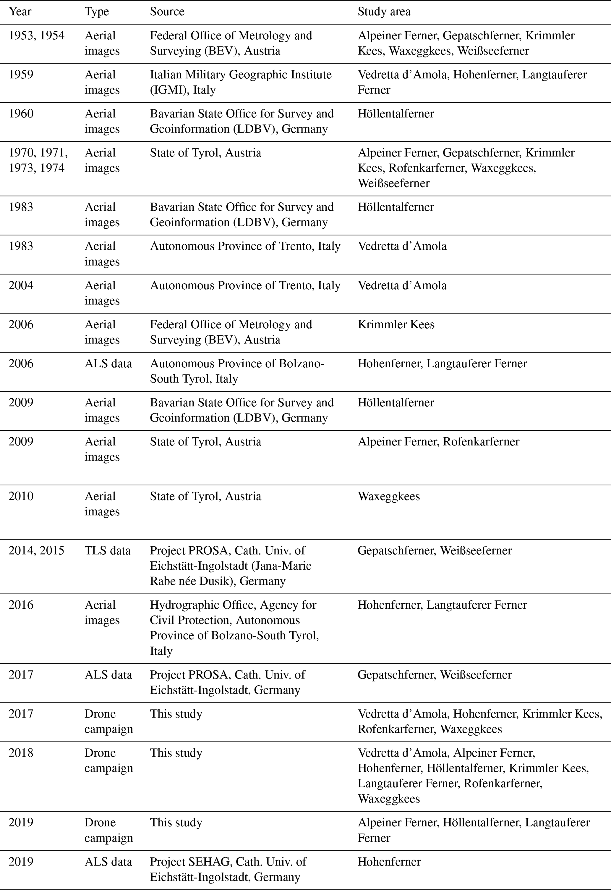
Moreover, drone images were taken of the 23 selected moraine sections for 2 consecutive years between 2017 and 2019. These were also the basis for the calculation of DEMs and orthophotos. For the moraine sections of two study areas, terrestrial laser scanning (TLS) data were used instead of drone images (see Table 2).

Besides the orthophotos generated from the named aerial image datasets, we also used old maps showing the former glacier extent together with descriptions and maps from the literature for mapping glacier extents (see Sect. 3.6.1). A complete list of the orthophotos, maps, and literature used can be found in Betz-Nutz (2021, 188–190).

3.2 Field survey

The field campaigns were conducted between 4 July 2017 and 4 September 2019, within the months July, August, and September of each year. For global referencing, we defined and measured ground control points (GCPs) on the selected moraine sections where drone images were later taken. As GCPs, large rocks on the moraine slopes were selected in an evenly distributed way and marked with crosses. However, on the steepest slopes, no GCPs could be set on the upper slope due to inaccessibility. Yet, on many moraine sections it was possible to access the ridge of the moraine and mark and measure GCPs there. On each moraine section, between 14 and 79 GCPs were marked and measured, depending on the size and terrain complexity of the slope.

The crosses marked on the stones were then surveyed using a total station by Leica Geosystems AG, TCRM1205 Type GDF121. As these measurements were conducted using the local coordinate system of the total station, at least three fix points around the total station were also measured using a Stonex S9III Plus Global Navigation Satellite System (GNSS) antenna for about 1.5 h per point to gather global coordinates. The recorded raw data were then post-processed by the Trimble CenterPoint RTX post-processing service. The local coordinates of the total station were then rotated into the geocentric coordinate system using the fix points and a coordinate transformation based on Euler angles. Finally, the GCPs were converted into the Universal Transverse Mercator (UTM) coordinate system (Zone 32N, EPSG 25832). In the field campaigns of following years, the GCPs that had already been marked and measured were used again (where still available). However, most GCPs and some fixed points were measured again as they were not found again or had moved.

After marking and measuring the GCPs, aerial photos of the moraine sections were taken by a DJI Phantom 4 Pro⁺ drone. Care was taken to achieve a high overlap between the images taken in the horizontal and vertical directions to enable good photogrammetric processing. The flight strips were parallel to the slope, and we attempted to keep the distance to the slope constant so that the marked crosses on the stones could be seen clearly. The mounted camera of the drone was positioned in such a way that the view direction was orthogonal to the slope surface and for that purpose it was also adapted during the flight. This means it had to be adjusted corresponding to the slope angle, which varies on the lateral moraines from the foot to the ridge. Between 396 and 1610 images were taken per moraine section.

3.3 Photogrammetric analysis

The archival aerial images and the drone images were used to generate DEMs via photogrammetric processing using structure from motion with multi-view stereo principle (SfM-MVS) in Agisoft Metashape Professional (https://www.agisoft.com/, last access: 10 March 2023). The background and workflow of using SfM-MVS has been explained in various earlier publications (Aber et al., 2019; Carrivick et al., 2016; Eltner et al., 2016; Smith et al., 2016; Westoby et al., 2012).

First, the drone images of each investigated moraine section were processed. After the calculation of the sparse cloud in Agisoft Metashape, the GCPs measured in the field (see Sect. 3.2) were set directly on the images as markers, and optimizations of the camera parameters were done several times. Subsequently, the dense cloud was calculated with high quality, and orthophotos were generated.

The historical digitized (scanned) images and the newer digital aerial images, all covering whole glacier forefields, were processed in the next step. As described in Stark et al. (2020) and Altmann et al. (2020), the historical images were pre-processed by (i) resizing the images so that each set of images had the same size in order to be associated with one camera, (ii) masking of the black border of each image, and (iii) adjusting the contrast for some of the images. In the following, the images were processed with the same standard workflow as the newer digital images. For global referencing, first the GCPs selected for the drone image campaign were applied to the newest aerial images, since these have the smallest differences from the drone survey and better image quality. Once having processed this newest aerial image dataset, we used the orthophotos and DEMs to select GCPs that are well distributed within the total glacier forefield and on the margins that could also be identified in the historical aerial image datasets. The GCP coordinates were extracted from the previously generated DEMs and applied to the historic aerial images.

3.4 Point cloud adjustment and calculation of DEMs of difference (DoDs)

Further processing of the points clouds was done in SAGA LIS (Conrad et al., 2015; https://www.laserdata.at/software.html, last access: 15 March 2023). After cropping the point clouds to the extent of the area of interest and removing outliers, the point densities of point cloud pairs selected for comparison were set to a similar value via 3D block thinning. We used the filter method “mean”, where a new point representing the mean value within the defined block is calculated. The horizontal and vertical spacing depends on the density of the point cloud and was selected to be between 0.1 and 1 m in our case. This enables a better adjustment of the point clouds and reduces the data amount (Mayr et al., 2018; Stark et al., 2020). In a next step, preliminary DEMs and DEMs of difference (DoDs) were employed to visually identify stable areas.

In the following, the points within these stable areas were used to optimize the co-registration of the point clouds using the tool “iterative closest point adjustment” (ICP) in SAGA LIS. Subsequently, the calculated transformation and rotation matrix for the stable areas was applied to the whole point cloud that should be adjusted. In some cases, after the first ICP the mean value of the DoDs was near zero, but systematic errors could be found in different parts of the model due to the fact that the ICP algorithm cannot eliminate complex, non-linear errors (cf. Bakker and Lane, 2017). Therefore, the affected point clouds were split into parts with either positive or negative deviations, and ICP was done separately before merging the adjusted subsets to one single point cloud.

After adjustment, raster DEMs were generated from the point clouds using the mean elevation of points for each raster cell. The resolution was 1 m or sometimes 1.5 m for the DEMs of the aerial images (2.5 m for the ALS data of South Tyrol) and 0.2 m for the drone-DEMs. Finally, DoDs were calculated by subtracting the two corresponding DEMs.

3.5 Error estimation

Despite accurate ICP adjustment, the calculated DoDs still have an uncertainty that has to be estimated when an erosion rate is calculated. The uncertainty assessment is based on stable areas, i.e. selected sections of the DoDs that had obviously and plausibly not experienced any surface changes, for example bedrock outcrops or flat, inactive, and sometimes vegetated lateral moraine sections. The DoD values within these areas nevertheless show non-zero values that are related to measurement uncertainties. Regarding the determination of the uncertainty, we have to distinguish between the accuracy (closeness of the two DEMs to each other) and the precision (variance within the model) of the measurement. We decided to use the standard deviation (precision) and the mean value (accuracy) of the DoDs in this study (cf. James et al., 2019).

The study of Anderson (2019) deals with the propagation of these errors into the volume or a mean change. He proposes the estimation and combination of two random errors (one spatially autocorrelated and one uncorrelated) and one systematic error. A test was done with four different DoDs of this study (representative combinations of DEMs generated from aerial images, drone images, ALS, and TLS) in order to quantify the different error types. The results show that the corresponding errors are very small (0.003–2.1 cm) (see Betz-Nutz, 2021, for more details), as the random errors cancel out over larger areas (Anderson, 2019), and the systematic error (mean) is small due to the previous ICP adjustment. However, we only sum negative values (gross erosion) in this study, and this means that an additional source of error is not considered, namely when the true elevation change is so small that random errors are likely to cause the sign of the true change to flip, meaning that areas with accumulation are wrongly treated as erosion (or vice versa) (Anderson, 2019). Thus, we believe that the real error in the DoDs is in fact higher than calculated with the above method. Due to this fact, Anderson (2019) states that thresholding must be applied prior to the propagation of the error values into the volume so that these small values are excluded from the analysis. However, we found that reasonable thresholding would also remove shallow but plausible erosion features (see Betz-Nutz, 2021, for more details). Thus, we limit ourselves to considering precision and accuracy calculated within stable areas as a metric to assess the quality of DoDs.

3.6 Investigation of geomorphic processes

We used the orthophotos, DEMs, and DoDs to qualitatively and quantitatively investigate geomorphological processes occurring on the moraine slopes.

3.6.1 Interpretation of DoDs and orthophotos

The DoDs and orthophotos were interpreted regarding the surface changes that have occurred. Since surface changes are clearly visible in DoDs, their spatial patterns give important hints about, for example, the types of the corresponding geomorphic processes. The orthophotos aid the interpretation of the patterns seen in the DoDs. Together, this enables an evaluation of what geomorphic processes are affecting and forming the lateral moraines.

Moreover, the DoDs are helpful for the mapping of glacier extents and the detection of melting dead ice. The detection of debris-covered ice, still in contact with the glacier or already isolated, is often difficult when looking only at the surface at one point of time, e.g. on an orthophoto. The use of DoDs can be very helpful for the detection of debris-covered ice as they show negative values for subsiding surfaces (Abermann et al., 2010; Schomacker, 2008). This enables the exclusion of areas affected by debris-covered ice from analyses of geomorphic processes and the computation of erosion rates.

Thus, for the glacier mapping back until the 1950s, DoDs were used supplementarily to the orthophotos. The glacier extents were mapped in a way that ice on the margins that is covered by debris but still in contact with the glacier as visible on DoDs is considered part of the glacier (see the example in Betz-Nutz, 2021, p. 71, their Fig. 12). For the mapping of earlier glacier extents, old maps and descriptions in the literature were used (see Sect. 3.1).

Regarding the detection of melting dead ice with the help of DoDs, there are some features that can help to differentiate it from the melting glacier and sediment erosion (see also Fig. 2). First of all, it is isolated from the glacier mass. Furthermore, melting dead ice is usually represented by relatively high values in the DoD compared to sediment erosion values. Moreover, melting ice does not appear punctually or linearly but is instead found over larger areas. Geomorphic processes such as landslides, in contrast, would change the texture of the surface, and retreated moraine ridges would be visible. Instead, melting ice below the surface inhibits the formation of rills or other forms due to the constant change in the surface due to thawing. Another point is that a surface depression caused by dead-ice melt-out lacks corresponding depositional features in the downslope, while eroded material would have been deposited somewhere below or a channel would have transported the sediment away. Thus, if a possible sediment erosion can be excluded by the analysis of these features, the melting of debris-covered ice is very probable.

Figure 2 Detection of debris-covered dead ice for the example of the Alpeiner Ferner: (a) orthophoto of 1954 and (b) 1954–1973 DoD (the aerial images of 1954 are from BEV, while those of 1973 are from the State of Tyrol, Austria).

3.6.2 Morphometric analysis

Moreover, we compared profile lines of different DEMs and calculated the gully depth of all moraine sections with gullies and the headward retreat rate on these slopes.

For the calculation of the maximum depth of the gullies, first the most recent DEM was used to calculate the flow accumulation, contour lines, and hillshade. On the basis of these datasets, lines were digitized orthogonal to the gully thalweg from one gully ridge to the next and in slope-parallel distances of about 1 m. Following this, the height differences between the ridge and the thalweg were measured, and the profile with the biggest height difference (i.e. the most deeply incised) was determined. Moreover, the slope gradient of the deepest point of the respective profile in the thalweg was determined. Its cosine was then used to correct the height difference in order to determine the incision perpendicular to the gully thalweg.

Nearly all moraine slopes with gullies show headward retreat. In order to gain insight into the rates of the headcut retreat, the lines connecting the gully headcuts were mapped using the oldest (1950s) and the newest (2018/2019) orthophotos as a base. In the next step, the minimum and maximum Euclidian distances between the headcuts on the old and new orthophotos were measured (see Fig. 3). Moreover, the mean headcut retreat rate was approximated as follows. If the area of the headcut retreat between the left- and right-most gully (area outlined in blue in Fig. 3) was a rectangle, then its area divided by its width would be the length (distance of headcut retreat). Figure 3 shows that the area is not a rectangle and therefore has no constant length, but as the width is constant between the two epochs, the result of the division represents an average length and is equivalent to the average distance of gully headcut retreat.

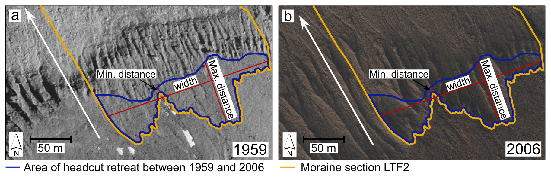
Figure 3 Measuring of the headcut retreat for the example of moraine section LTF2: (a) orthophoto of 1959 and (b) orthophoto of 2006 (aerial images of 1959 are from IGMI, and the 2006 orthophoto was provided by the Autonomous Province of Bolzano-South Tyrol).

3.6.3 Quantification of erosion rates

To enable a comparison of the morphodynamics on the lateral moraines, it was necessary to define comparable areas and time periods for the different study areas and moraine sections. Due to different sizes of the moraine sections and different proportions of the erosion, transport and deposition areas, the erosion rates were only quantified using the erosion areas on the upper slopes of the selected moraine sections, representing the main areas of erosion.

For this reason, the erosion area was mapped on each moraine section. The upper border of each erosion area was either the moraine ridge or the headcut of the gullies present on the slope. The lateral borders were mostly equal to the moraine section outline (see Sect. 2). The lower border of the erosion areas was drawn at the transition from the erosion to the transport area, which corresponds to the downslope end of the gully sidewalls on gullied slopes (see Fig. 8).

As slope areas including melting dead ice would falsify the calculation of the real sediment erosion, dead-ice areas were excluded from the mapped erosion areas. In cases where it was not possible to clearly delimit the dead-ice-affected area from the ice-free slope, no erosion area could be defined for these moraine sections.

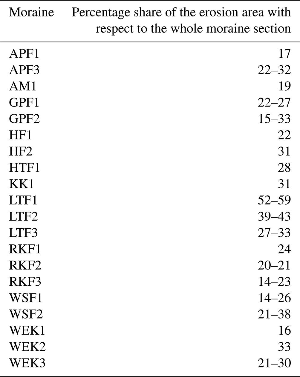
Wherever possible and reasonable, the outlines of the erosion areas were used for several DoDs of the same moraine section, as this ensures the best comparability. However, for the case of extensive changes over time, the erosion areas had to be defined independently for different DoDs in order to include areas formerly featuring dead-ice or glacier areas or newly formed erosion areas in younger DoDs. The proportion of erosion area compared to the total area of the moraine sections can be seen in Table 3.

Table 3 Proportion of erosion area compared to the total area of the moraine sections.

Subsequently, all DoD cells with negative values within the erosion areas were summed up, multiplied by the cell size (see Sect. 3.4), and divided by the size of the erosion area and the number of years spanned by the respective DoD. Hence, the resulting erosion rate represents a mean annual surface elevation change (in cm a⁻¹) within a certain period.

In order to improve the comparability and to facilitate the interpretation of the temporal evolution of erosion rates, the DoDs were allocated to three general time periods of similar length based on the majority of the available image datasets.

• Time period 1. This period includes all DoDs from the 1950s to the 1970s.

• Time period 2. This period includes all DoDs from the 1970s to the 2000s. DoDs ranging from the 1950s and 1960s to the 2000s are allocated to period 1 and 2 (same erosion rate for both time periods).

• Time period 3. This period includes all DoDs from the 2000s to 2018/2019. The erosion values calculated using several DoDs within this time period were summed up and divided by the years covered by the entire period.

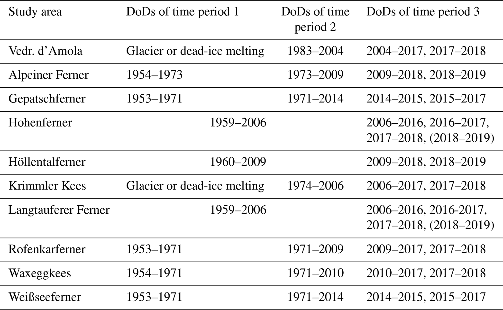
A list of all DoDs used for the calculation of erosion rates and their attribution to the time periods can be found in Table 4.

Table 4 DoDs used for the calculation of the erosion rates and their attribution to the defined time periods 1–3. Note that some moraine sections of the DoDs covering the entire forefields are affected by dead ice in some time periods (see Fig. 10), and for some moraine sections additional drone images were acquired (years in parentheses).

3.7 Analysis of possible influencing factors on morphodynamics

In order to investigate possible factors influencing the morphodynamics on lateral moraines, we conducted an analysis including the entire defined glacier forefields.

For this analysis, the most recent DoD covering the entire respective glacier forefield was used, mainly representing the second analysed time period ranging from the 1960s, 1970s, or 1980s to the 2000s. The latest available DEMs of the entire glacier forefields, which are from the 2000s (see Table 2 for the exact year of the respective aerial images), formed the basis for the derivation of the slope angle. For better comparison, the resolution of all models was set to 1 m for this analysis. All areas with bedrock and areas with a glacier or dead ice were excluded from the analysis, as were river channels, forest areas, and human infrastructure.

As mentioned before (Sect. 1), morphodynamics are assumed to depend on the time since deglaciation (amongst other factors). Deglaciation is understood in this study to be the complete melting of the glacier at a particular location, but this does not necessarily include the melt-out of dead ice or ice-cored moraines. In order to analyse the relationship between the erosion and time since deglaciation, an interpolation of the mapped glacier extents was necessary to estimate a value for the time since deglaciation for each raster cell. For this purpose, we gridded the mapped glacier outlines and calculated a distance grid showing for each pixel the Euclidian distance to the next pixel of a glacier outline. In the next step, we used two distance grids of subsequent glacier extents to calculate the year of deglaciation for each pixel using a linear interpolation of the respective dates of glacier extents based on the distance ratio. After this was calculated for each pair of distance grids, all grids with the years of deglaciation were merged. Moreover, the years since deglaciation were approximated by the difference between the date of deglaciation of the respective raster cell and the mean year of the time period spanned by the used DoD. These interpolated times of deglaciation were also used to define the year of complete deglaciation for each moraine section (youngest year when the foot of the slope was free of glacier ice).

4 Results and discussion

4.1 Results of the error estimation

For the quality assessment of the different DoDs, an error estimation was conducted within stable areas, which revealed a wide range of errors depending on the type of dataset. Figure 4 shows boxplots with the distributions of the mean values and standard deviations of the DoDs. Both parameters are highest for the DoDs based on aerial images. The absolute value of these mean values ranges between 0.2 and 18.4 cm within this group, and the standard deviation ranges between 12.2 and 76.5 cm. The large differences within this type of DoD can be explained by the different quality of the aerial images (e.g. flight height, image resolution) and the resulting elevation models. Regarding the interpretation, we took care when comparing the erosion rates of these models with high uncertainties with erosion rates of other periods or moraine sections and reflected this in the interpretation of the results. Within the group of DoDs generated from a DEM based on aerial images and a DEM based on drone images, the absolute value of the mean ranges from 0.03 to 4.8 cm, and the standard deviation ranges from 5.3 to 24.6 cm. This outlier of 24.6 cm can be explained by an aerial image dataset of low quality within the Vedretta d'Amola area (2004). However, the variance is much lower within this group. An even lower variance is visible for the DoDs based on drone image datasets, where the absolute value of the mean is 1.8 cm at most and the standard deviation is between 1.3 and 6.5 cm. These lower errors can be explained by the better quality of the drone images in comparison to the aerial images (especially the older ones). The uncertainties determined for the aerial image datasets are comparable to the values reported by Stark et al. (2020) and Micheletti et al. (2015a), and this is also the case for the DoDs based on drone images (e.g. Smith and Vericat, 2015).

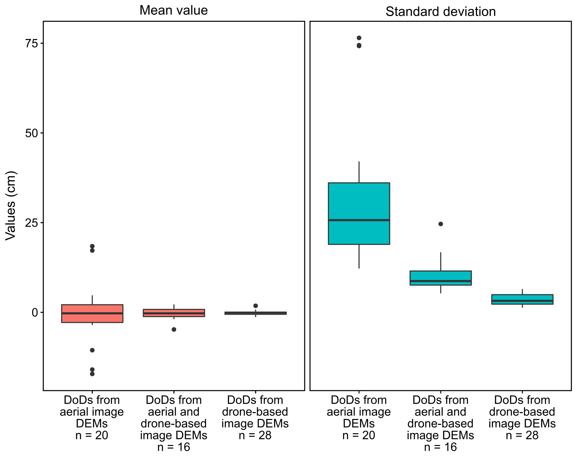
Figure 4 Boxplots showing the distribution of the mean values and standard deviations for different types of DoDs: DoDs from aerial image DEMs, DoDs from aerial and drone-based image DEMs, and DoDs from drone-based image DEMs.

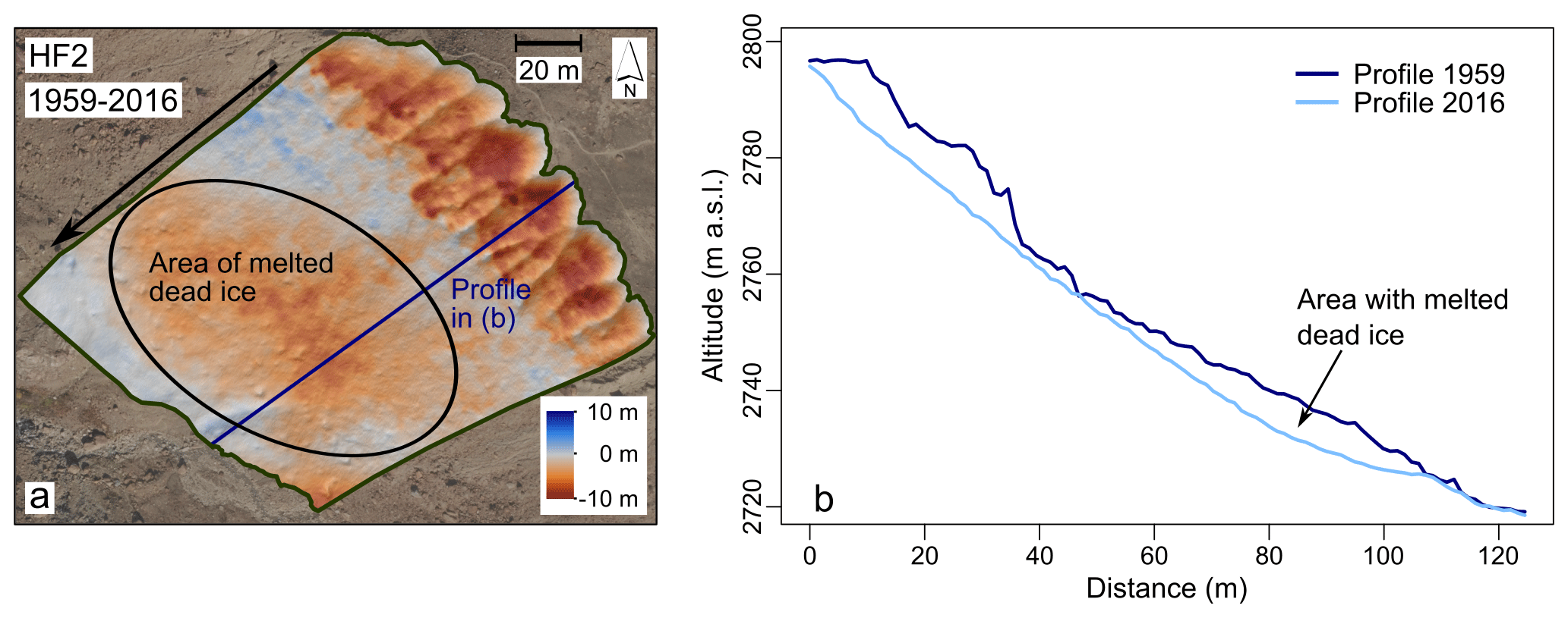
Figure 5 Reaction of lateral moraine slopes to dead-ice melting for the example of moraine section HF2: (a) 1959–2016 DoD and (b) length profile through the DEMs of 1959 and 2016 (aerial images of 1959 are from IGMI, while the 2016 images are from the Hydrographic Office of the Agency for Civil Protection of the Autonomous Province of Bolzano-South Tyrol).

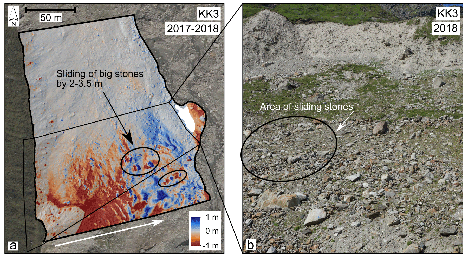
Figure 6 Reaction of lateral moraine slope to dead-ice melting for the example of moraine section KK3: (a) 2017–2018 DoD and (b) image taken from the foot of the moraine slope towards the ridge on 1 August 2018, a rough outline of which is marked in (a).

4.2 Geomorphic processes triggered by dead-ice melt

Melting dead ice is widespread within the investigated glacier forefields and thus in the lateral moraines; it was found in all but one glacier forefield, namely that of the Höllentalferner. Both the long time span and the low elevations in which dead-ice melt-out was detected in some forefields are surprising. In the forefield of the Alpeiner Ferner, at moraine section APF2, dead ice is detectable from 1953 to 2019, i.e. for 65 years, at an altitude of about 2500–2600 m a.s.l. In the forefield of the Krimmler Kees, dead ice existed for several years (at least from 2004 to 2018) at an altitude of about 2000–2200 m a.s.l. This shows that the lateral moraines are strongly affected by melting dead ice. In the following, we present two examples of different geomorphic reactions of lateral moraine slopes to melting dead ice.

The first one is a moraine slope in the forefield of the Hohenferner in the Martell Valley, where dead ice was melting on the middle and lower slope between 1959 and 2016 (Fig. 5a). When comparing the length profiles of 1959 and 2016 (Fig. 5b), a depression of up to 7 m depth is visible in the middle and lower slope part, created due to the subsidence of the sediment after ice melting. Moreover, an increase in the slope gradient of about 10^∘ is detectable in the area where dead ice melted. In total, the surface subsidence leads to a withdrawal of support for the steep upper slope and thus contributes to the destabilization of the slope. It can be supposed that the incision of gullies on the upper slope has been enhanced by the subsidence on the middle and lower slope. The higher surface roughness in 1959 in comparison to 2016 is supposedly caused by sediment-covered dead-ice patches undulating the surface and the lower DEM quality of 1959.

The moraine section KK3 in the forefield of the Krimmler Kees shows a different reaction to melting dead ice on the middle and lower slope. On this slope, no incision of gullies has occurred, and in general hardly any linear erosion is detectable. It is possible that dead ice, which reached further up the slope than it does today, prevented the formation of linear erosion forms. Instead, due to the melting dead ice, the whole slope seems to slide down, which is detectable from the high negative values on the middle slope and the slightly positive values of the DoD on the lower slope, which are probably partly compensated for by melting ice on the lower slope (Fig. 6a). On the lower slope, the sliding is also clearly visible due to some bigger rocks that slid down by 2–3.5 m. We infer from the existence of vegetation (Fig. 6b) that no geomorphic processes occur directly on the surface because otherwise the vegetation would have been affected.

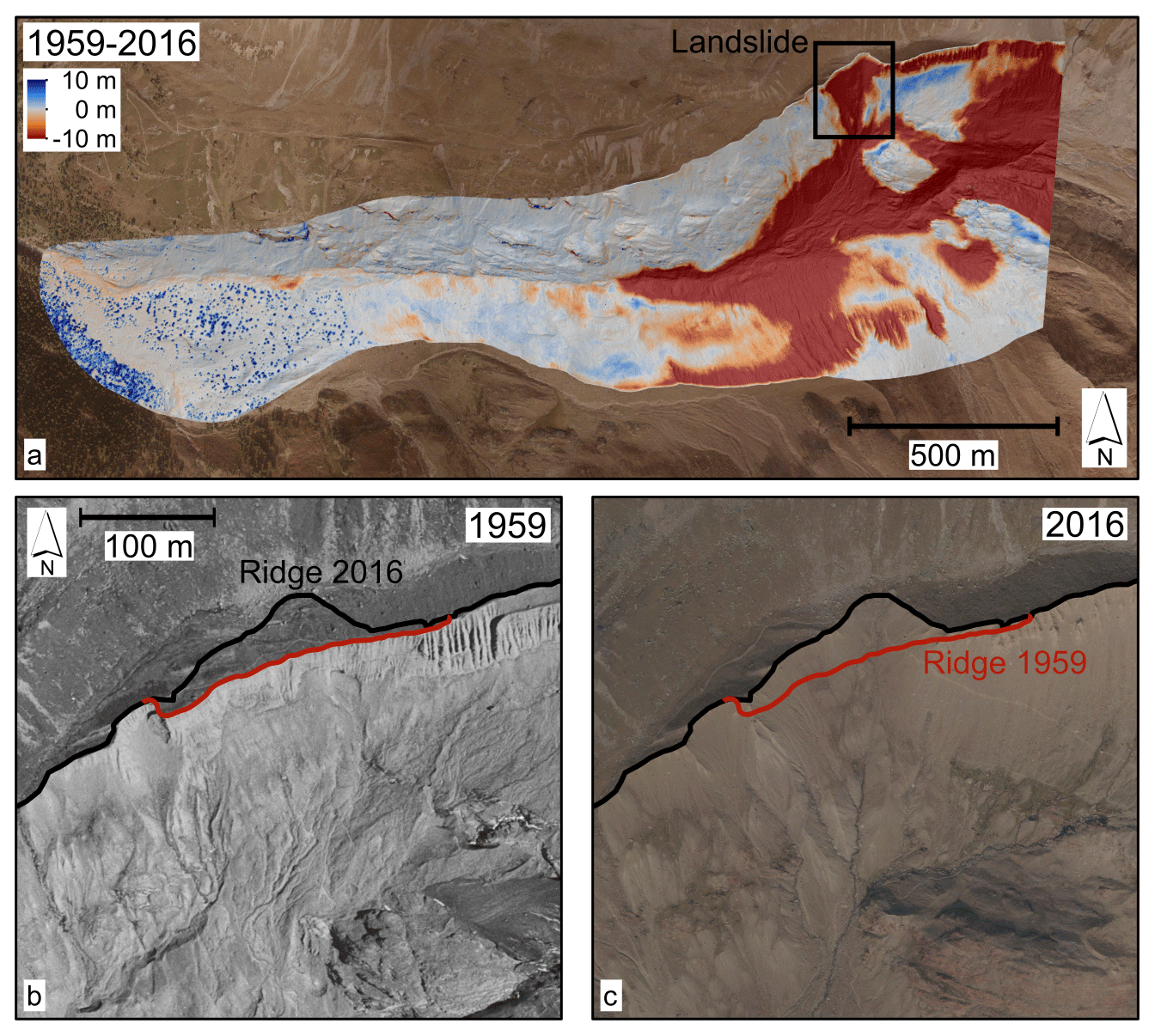
Figure 7 Landslide on the lateral moraine of Langtauferer Ferner: (a) 1959–2016 DoD of the entire glacier forefield, (b) aerial image of 1959, and (c) aerial image of 2016 (aerial images of 1959 are from IGMI, while the 2016 images are from the Hydrographic Office of the Agency for Civil Protection of the Autonomous Province of Bolzano-South Tyrol).

Looking at all investigated glacier forefields, the subsidence due to melting dead ice causes the largest height differences in our DoDs (cf. Sailer et al., 2012) aside from glacier melting. A retarding influence on the stabilization of the moraines by the melting ice and the induced geomorphic processes can be strongly supposed, as also assumed by Lukas (2011) and shown in Ravanel et al. (2018).

4.3 Geomorphic processes and landforms

Based on the interpretation of (i) the spatial pattern of negative and positive values of the DoDs and (ii) orthophotos, different types of geomorphic processes and landforms on the moraine slopes could be detected. In the following, three main types of slopes with typical predominant geomorphic processes and landforms will be discussed.

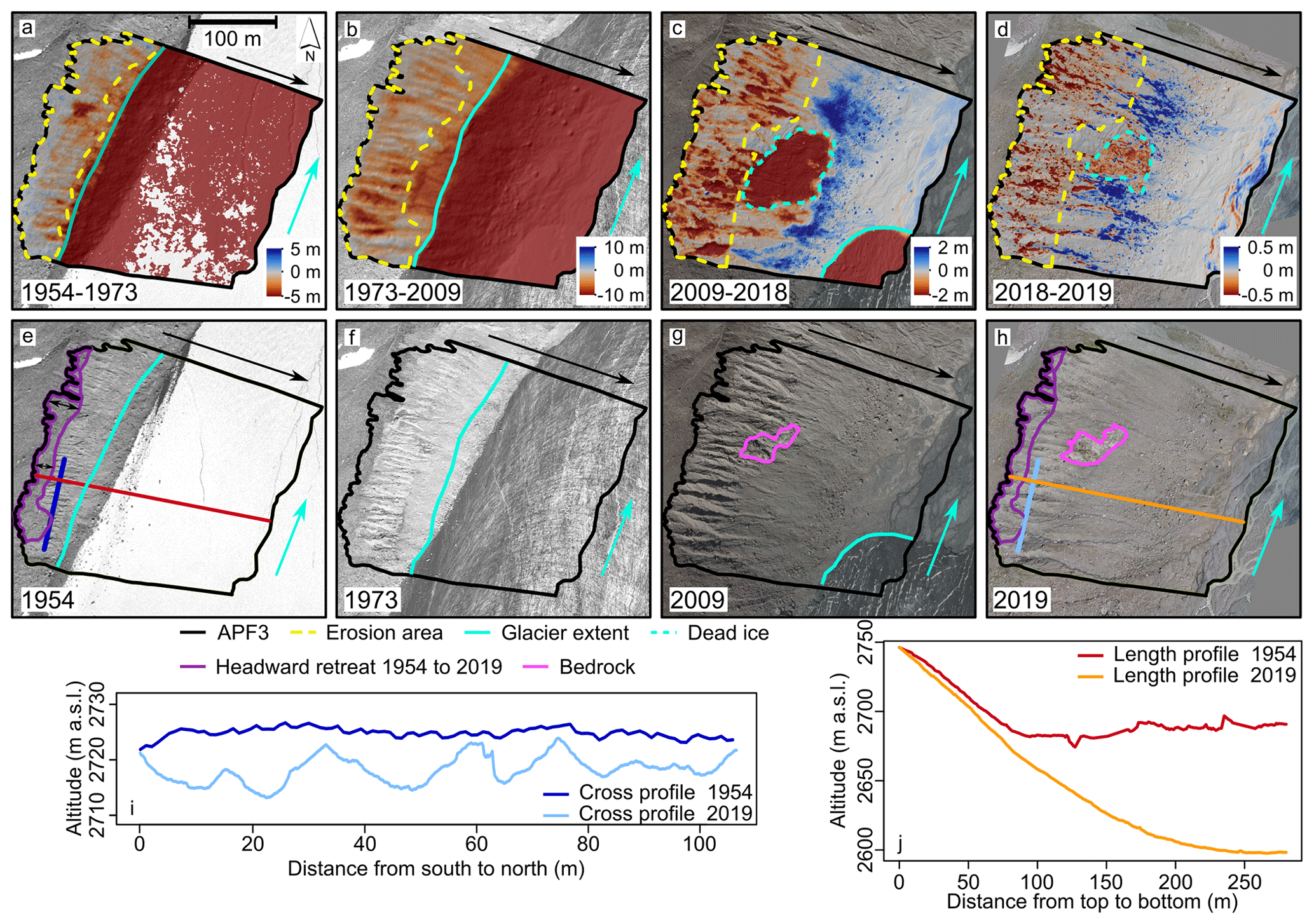
Figure 8 Development of deeply incised gullies for the example of moraine section APF3 in the Alpeiner Ferner forefield: (a–d) DoDs of moraine section APF3 for 1954–1973, 1973–2009, 2009–2018, and 2018–2019, with markings showing the erosion area (dotted yellow line), glacier extent (cyan line), glacier flow direction (cyan arrow), and dead ice (dotted cyan line) and black arrows indicating the downslope direction; (e–h) orthophotos of APF3 for 1954, 1973, 2009, and 2019, with lines showing the length (blue) and cross profiles (red/orange) and a bedrock outcrop (magenta); (i) cross profiles through APF3 for 1954 and 2019; and (j) length profiles along APF3 for 1954 and 2019 (the aerial images of 1954 are from BEV, and those from 1973 and 2009 are from the State of Tyrol, Austria).

4.3.1 Landslides

In some of our study areas, landslides occurred within the first study period beginning in the 1950s. One example in the forefield of the Langtauferer Ferner has been detected on the 1959–2006 DoD and the orthophotos of 1959 and 2016 (Fig. 7b and c). Figure 7a shows the 1959–2016 DoD (for reasons of better resolution). The landslide has a width of 145 m and the depth, meaning the difference between the surfaces of 1959 and 2016, is up to 30 m in some areas. Ongoing erosion following the landslide could have caused further incision, and thus the original landslide may have been slightly smaller. The landslide displaced the moraine ridge backwards by up to 40 m (orthophotos in Fig. 7b and c). As the DoD shows, the areas below the landslide on the valley bottom were still affected by glacier and dead ice melting within this period. This leads to the assumption that the landslide could have been a reaction to changing erosional base levels. It is conspicuous that other glacier forefields that feature big landslides, such as the Gepatschferner with a landslide of a similar size, were also substantially covered in ice on the valley bottom at that time. Other glacier forefields that were already deglaciated at the starting point of our investigations, however, showed no landslides during our observation period, and additionally the earliest orthophotos or DEMs do not show indications of displacements of moraine ridges prior to ca. 1950 that could correspond to landslides. In the forefields of the Langtauferer Ferner and the Gepatschferner, landslides seem to be the dominant processes during deglaciation regarding the erosion volume, as was also observed in the study of Cody et al. (2020) in New Zealand.

Gravitational deformation of moraines, leading to large gaps in the moraine crest during glacier recession, is also reported by Hugenholtz et al. (2008) in the Canadian Rocky Mountains. Moreover, Blair (1994) describes slope failure of lateral moraines and valley walls in New Zealand as being a consequence of the accelerated ablation rates of the glacier.

4.3.2 Slopes with deeply incised gullies

Many of the investigated glacier forefields exhibit lateral moraine sections with heavily gullied upper slopes. All of these moraine slopes were affected either by a melting glacier or melting dead ice on their middle and lower slope within our observation period, except for two moraine sections that had already deglaciated soon after 1900. At several moraine sections, the formation of the heavily incised gullies could be observed beginning with our first DoDs from the 1950s to the 1970s (APF3, GPF1, GPF2, HF2, KK2, LTF2, LTF3, WSF2, for the location of the moraine sections see Fig. 1). On some sections, however, gullies were already present in the 1950s (beginning of observation period), and they do not seem to have experienced further incision since then (HTF1, WSF1, WEK2, WEK3). The moraine section APF3 in the forefield of the Alpeiner Ferner serves as an example of gully formation since the 1950s (Fig. 8). Erosion rates are presented in Sect. 4.4.

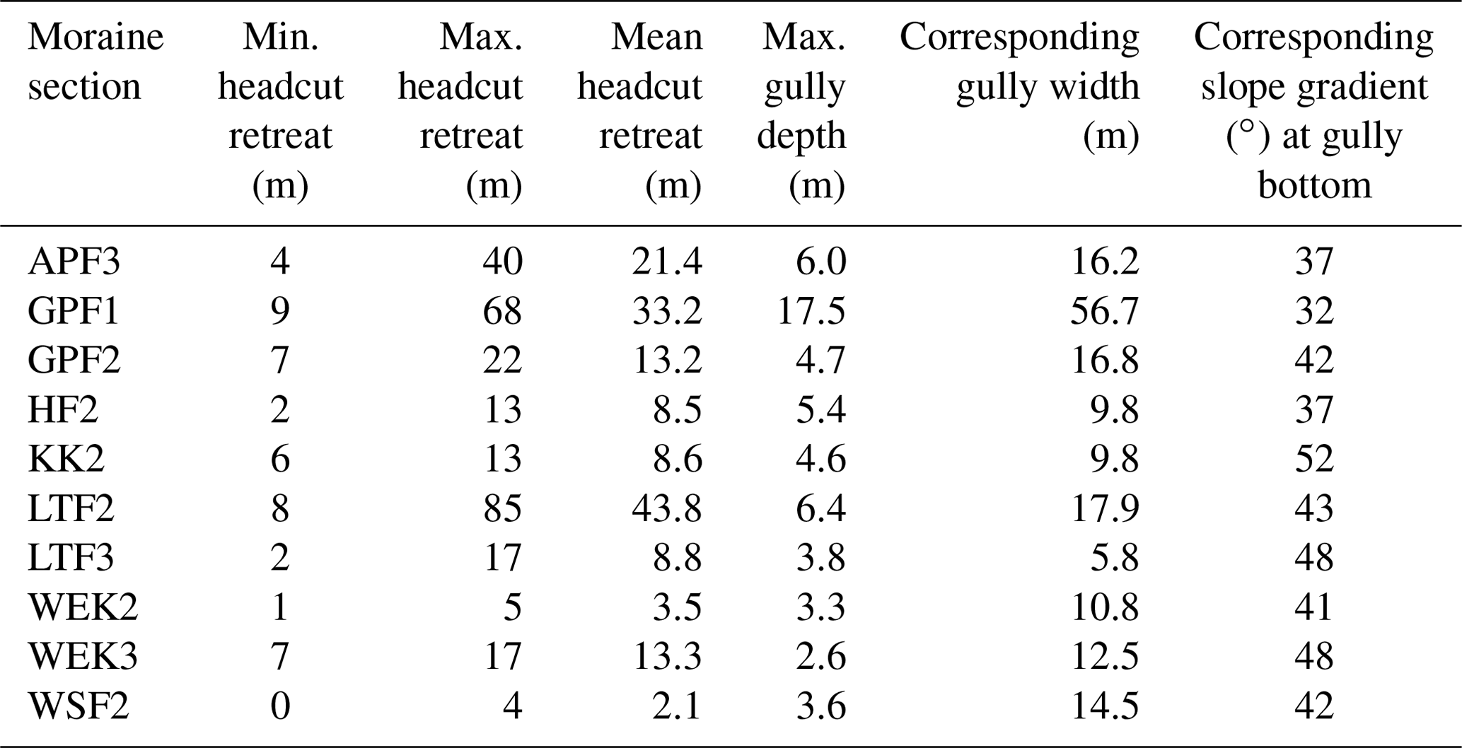
Table 5 Headcut retreat minima, maxima, and mean values between 1953, 1954, or 1959 (oldest available DEM) and 2018 or 2019 (newest available DEM) for each gullied moraine section and maximum gully depth, corresponding gully width, and corresponding slope gradient at the gully bottom for the most deeply incised gully on the respective moraine section.

The orthophoto of 1954 (Fig. 8e) and a cross profile through the DEM of 1954 (Fig. 8i) show that at that time only small rills were present at the upper slope, whereas the lower and middle slope were covered by the glacier in 1954. As the 1954–1973 DoD shows (Fig. 8a), erosion took place in these rills, presumably mainly linear fluvial erosion. The orthophoto of 1973 (Fig. 8f) already shows an enlargement of the rills that became gullies over time. On the 1973–2009 DoD (Fig. 8b), dominated in the middle and lower slope parts by glacier melt, it is also visible that, in addition to an incision of the rills due to linear erosion, a widening due to erosion on the gully sidewalls occurred. It can be assumed that, in addition to fluvial erosion, small-scale gravitational processes such as sheet erosion by snow gliding and denudation also lead to the gully widening. The DoDs of 2009–2018 and 2018–2019 (Fig. 8c and d) show that debris flows have become an important process that causes further gully incision and widening. The slope steepened from 1954 to 2018 from 36.9 to 43.5^∘ and the glacier nearly completely melted in the meantime (see the comparison of the length profiles in Fig. 8j). In 2019, a gully depth of about 6 m could be measured (see the cross profile in Fig. 8i). The accumulated debris flow material is visible on the lower slope part, right before reaching the channel, indicating poor hillslope–channel coupling in this place. The erosion on the gully heads, mainly happening after 1973, leads to the headward retreat of the erosion area (marked in purple in Fig. 8e and h). This retreat amounts to between 4 and 40 m and is easily possible on this moraine slope as it has no sharp ridge; the slope continues upward into a ground moraine of an earlier glacier flowing from the west to the northward-flowing main Alpeiner Ferner glacier tongue. It can be assumed that this favours the ongoing intense erosion and prohibits stabilization. An influence of the dead ice that is detectable on the 2009–2018 and 2018–2019 DoDs on the geomorphic activity is not clear in this case, as above the dead-ice area is also a bedrock outcrop that has been visible since 2009 (magenta area in Fig. 8g and h) and that contributes to stabilization.

These observed processes and the gully development on the moraine slopes in this study are consistent with the observations of, e.g. Dusik et al. (2019), Neugirg (2016), and Wetzel (1992) on similar slopes. Fluvial erosion starts with the formation of rills. Once the rills are bigger, loose material from the sides and headcuts is deposited in the rills, e.g. by snow gliding. Finally, small debris flows evolve from this loose material, supposedly mainly during heavy rainfall in summer, and contribute to a widening of the rills to gullies. It seems that these small debris flows are the dominant processes of sediment transfer on slopes with deeply incised and widened gullies in our study, as previously reported (cf. Ballantyne, 2002b; Cody et al., 2020; Curry et al., 2006; Dusik, 2020; Wetzel, 1992).

Table 5 shows an overview of all gullied moraine sections with respect to (i) the headcut retreat of the gullies (minimum, maximum, and mean for each moraine section) and (ii) the gully width, the gully maximum depth, and the gradient of the gully thalweg of the deepest gully. A maximum headcut retreat of 85 m could be measured on a moraine section in the Langtauferer Ferner forefield (LTF2), followed by a moraine section in the Gepatschferner forefield with a maximum retreat of 68 m (GPF1). The latter slope also stands out regarding the maximum gully depth. A very big gully on this moraine slope has a maximum depth of 17.5 m. This is also due to the relatively low slope gradient of 32^∘ and the high gully width of 56.7 m. The gullies on the other moraine sections show maximum depths from 6.4 m (LTF2) down to 2.6 m (WEK3).

A collapse or widening of the gullies until a levelling of the slope occurs, as described in Curry et al. (2006) based on the comparison of moraine sections with different age since deglaciation, cannot be reproduced with the data in this study. Only some gullies show less activity over time and eventually no longer any incision (WSF1, WEK2, WEK3, HTF1); however, they do not collapse, and the slope is not levelled. As already compared by Betz et al. (2019), where the moraine sections LTF2, LTF3, and HF2 were analysed in a similar way to in Curry et al. (2006), these moraine sections do not show the progression of gully development with increasing age as described by Curry et al. (2006). Neither is a maximum gully incision reached 5 years after deglaciation nor do the gullies widen only 80–140 years after deglaciation. Dusik et al. (2019) also could not reproduce the gully development assumed in Curry et al. (2006).

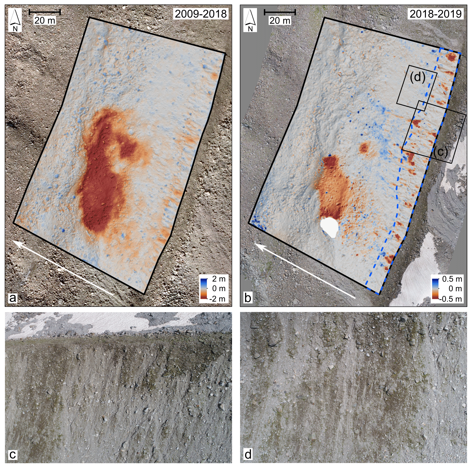
Figure 9 Slope with shallowly incised gullies or rills illustrated for moraine section APF2 in the Alpeiner Ferner forefield: (a) 2009–2018 DoD (the aerial images from 2009 are from the State of Tyrol, Austria), (b) 2018–2019 DoD with the erosion area (blue), and (c, d) drone images of the slope from 1 August 2019.

4.3.3 Slopes with shallowly incised gullies or no incision

In addition to moraine sections with deeply incised gullies like the one explained in Sect. 4.3.2, there are lateral moraine sections that show only very shallowly incised gullies, rills, or even no incisions at all. Some of these exhibit denudation and sheet erosion, while others show no erosion at all. One lateral moraine section in the Alpeiner Ferner forefield, APF2, is an example showing only shallowly incised rills (Fig. 9). Although there is dead ice melting on the middle slope, the upper slope (41^∘ slope gradient) does not show heavy gullying. Instead, mostly fluvial processes and small slides, and possibly also small debris flows of short length, are occurring, as can be especially seen in the 2018–2019 DoD in Fig. 9b. It can be assumed that the melting dead ice, which also reached up to the upper slope until recently, as suggested by the 2009–2018 DoD in Fig. 9a, inhibited the incision of linear forms due to the constant, areal melting of the ice. Without gully incision and headcut erosion, a headcut retreat of the moraine ridge is also missing here. A stabilization of the slope, however, has not yet occurred as the already existing grass vegetation is destroyed again by the geomorphic processes (images in Fig. 9c and d).

Lateral moraine slopes with these kinds of geomorphic processes, i.e. mainly fluvial processes and small slides, can be found in almost all investigated glacier forefields. However, they mostly do not show melting dead ice any more. Some of these moraine slopes show ongoing activity, but some also show a decrease in activity and signs of stabilization such as vegetation growth. The development of the corresponding erosion rates is presented in the following section.

4.4 Erosion rates

The temporal development of the morphodynamics and thus the erosion rates differ between the investigated lateral moraine sections. Decreases in erosion rates, stagnation of erosion rates, and increases in geomorphic activity could all be detected. Figure 10 compares the erosion rates of the 20 moraine sections for which erosion rates could be calculated in at least two of the three time periods (1950s–1970s, 1970s–2000s, 2000s–2018).

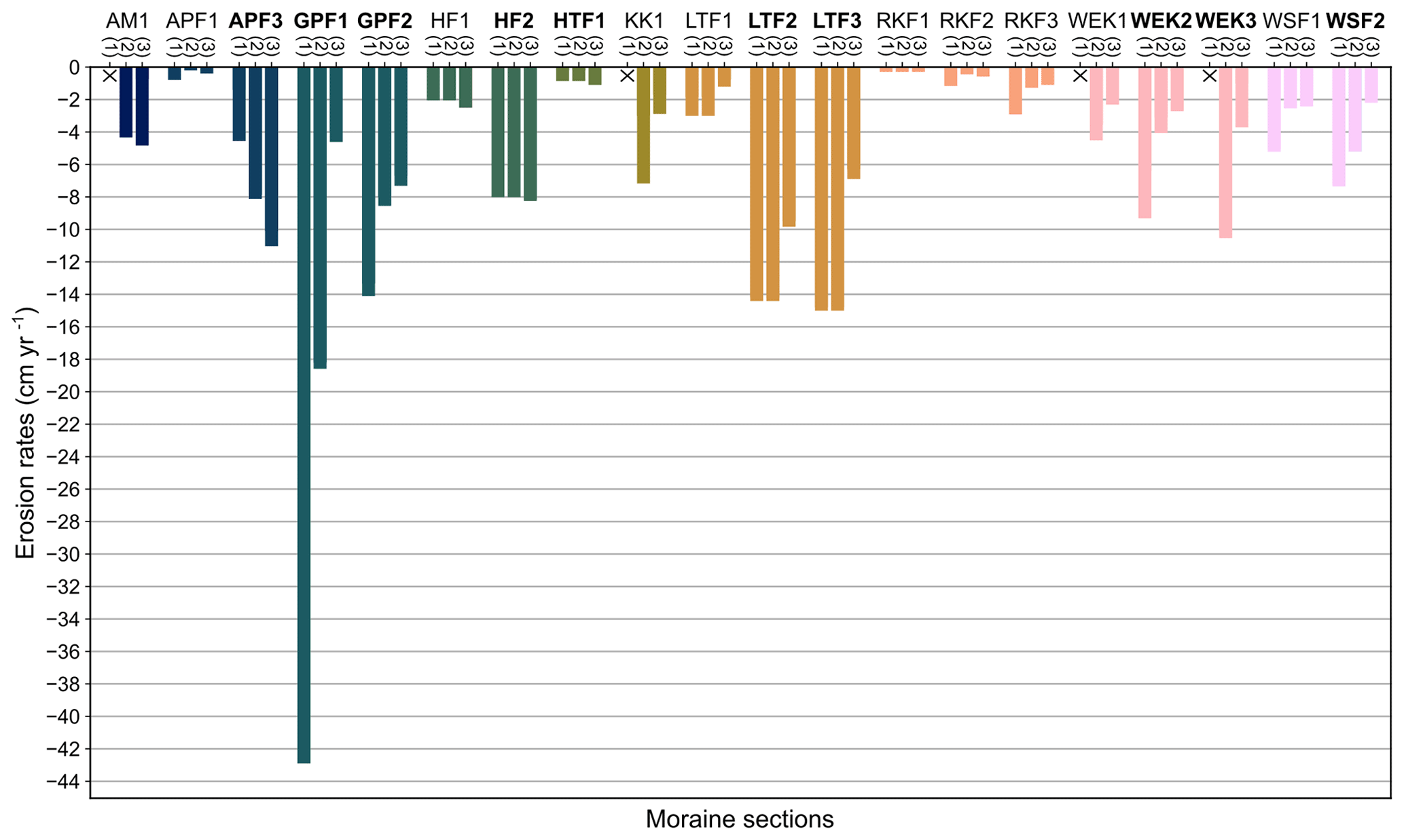
Figure 10 Erosion rates for 20 investigated moraine upper slopes for the three time periods (1) 1950s–1970s, (2) 1970s–2000s, and (3) 2000s–2018 (see Table 4 for specific DoDs). Moraine sections written in bold represent upper slopes with deeply incised gullies (colour map batlow10 from Crameri et al., 2020).

The highest erosion rates could be found for the moraine slopes with deeply incised gullies as described in Sect. 4.3.2 (names marked in bold in Fig. 10). Within this group, the highest erosion rate was detected on moraine section GPF1 with nearly 43 cm yr⁻¹ in the first time period. At this time the glacier (Gepatschferner) and dead ice melted on the slope foot and also partly on the middle slope. Another moraine section in the Gepatschferner forefield (GPF2) also shows high rates of 14 cm yr⁻¹ in this first observed time period. Also, two moraine sections in the Langtauferer Ferner forefield (LTF2, LTF3) have an erosion rate of 14–15 cm yr⁻¹ in the period from 1959 to 2006, where LTF2 in particular was heavily influenced by the melting glacier. This means that the highest erosion rates can be detected in the phase of strong glacier melting on the slope foots accompanied by initial gully erosion and, on some slopes, by landslides (see Sect. 4.3.1). After this initial gully formation and glacier melting, the erosion rate decreases to lower than 10 cm yr⁻¹ but stays at a high level, with more than 4 cm yr⁻¹ of erosion even decades after deglaciation in time period three. The gullied moraine section HF2 shows a slight increase or at least stagnation over many decades (8.0 cm yr⁻¹ in 1959–2006, 8.3 cm yr⁻¹ in 2006–2018), while APF3 even exhibits a clear increase in erosion rate from period one to three (10 cm yr⁻¹ in 2009–2019). It deglaciated completely only recently (in 2012) and is still influenced by melting dead ice, which is likely to influence the activity. Only on three gullied slopes with less deeply incised gullies did the erosion rates decline below 4 cm yr⁻¹, with rates between 2.2 and 3.7 cm yr⁻¹ in the third period (WSF2, WEK2, WEK3). These slopes already deglaciated in the 1930s, and the gullies were well developed in 1953, meaning that, unlike on other slopes, the gullies have stabilized over the decades. Overall, most of the gullied slopes show decreasing but ongoing high activity even after decades, while only a few seem to stabilize after many decades.

The erosion rates of the group of gullied slopes is comparable with erosion rates reported in literature, except for HTF1, which shows only very little activity. For the erosion in gullies on lateral moraines, studies in Norway determined 1.9–16.9 cm yr⁻¹ (Ballantyne and Benn, 1994; Curry, 1999), a study in Switzerland determined 4.9–15.1 cm yr⁻¹ (Curry et al., 2006), and a study in Austria determined 2.9–3.4 cm yr⁻¹ (Dusik, 2020). These lateral moraines for which erosion rates are reported had been deglaciated for 43–79 years at the time of observation, which is comparable with our investigated moraine sections. However, it must be kept in mind that the methods to calculate the erosion rates differ between the studies. While, e.g. in Curry et al. (2006) and Curry (1999) the erosion rates were deduced from the volume of the existing gullies, assuming that this represents the eroded volume, in Dusik (2020) and in this study the erosion rates were calculated based on the height differences detectable in the DoDs.

The slopes with shallow gullies, rills, or no gullies show lower erosion rates, and more signs of stabilization can be found on these slopes. In the first observed time period, erosion rates of up to 7 cm yr⁻¹ (KK1) occurred on these slopes; however, on most of the slopes the rate was below 5 cm yr⁻¹ in all time periods. In the third period, the erosion rate decreased to around 1–3 cm yr⁻¹ on the moraine sections KK1, LTF1, RKF3, WEK1, WSF1, and RKF2. The highest activity in the third period was detected on AM1 with 4.8 cm yr⁻¹, whereas HF1, which is characterized by sheet erosion by snow, shows a constant erosion rate of 2.1–2.5 cm yr⁻¹. Reasons for the overall lower activity of these slopes can be seen in the longer time since deglaciation and lower slope angles due to their location being closer to the LIA maximum glacier extent (see Sect. 4.5.1 and 4.5.2). The rates are comparable with the ones in Dusik (2020) on lateral moraines at the Weißseeferner (Austria) without gully formation with 0.8–1.7 cm yr⁻¹ (Dusik, 2020).

4.5 Influencing factors on morphodynamics

4.5.1 Time since deglaciation

As the time since complete deglaciation and dead-ice melting on the moraines determines how much time has passed for the adjustment of lateral moraines and for landform evolution on the hillslopes, this parameter is important for the analysis of the morphodynamics.

In Fig. 11, the mean erosion rates of the moraine sections in time period 3 (see Table 4 for specific DoDs) are plotted against the years of their deglaciation (for the interpolation method for years of deglaciation, see Sect. 3.7). Here, the end of dead-ice melting is not considered, as this is not detectable until the 1950s, the time of the first DEMs. Besides the erosion rates and the time of deglaciation, it is indicated if the moraine sections are characterized by deeply incised gullies or by only shallow (or no) gullies (filled and empty symbols, respectively). It can be recognized that moraine sections that deglaciated later show higher erosion rates. The moraine sections with low erosion rates (below 2 cm yr⁻¹) already deglaciated before 1950, with the exception of one moraine section that deglaciated in 1990 (RKF3). The moraine slopes with the highest erosion rates (more than 4 cm yr⁻¹), however, deglaciated after 1950, again with one exception (LTF3 deglaciated in 1911). Moreover, a trend can be seen that moraine sections showing only shallowly incised gullies or no gullies deglaciated earlier, while those with deeply incised gullies deglaciated later.

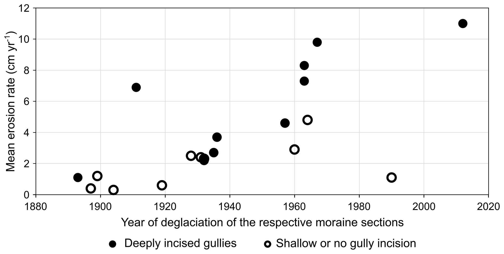
Figure 11 Mean erosion rates in time period 3 (see Table 4 for specific DoDs) depending on the years of deglaciation of the moraine sections with deeply incised gullies and shallow (or no) gully incision.

Besides this analysis of the investigated moraine sections, an analysis based on all grid cells within the 10 glacier forefields was conducted (see Sect. 3.7). Figure 12 shows the sum of the annual erosion volume categorized by 20-year groups of the time difference between deglaciation and the mean year of the respective DoDs, divided by the entire area that deglaciated in the respective time period. It is conspicuous that grid cells that deglaciated between the mean year of the respective DoD and up to 20 years before (mainly deglaciated between 1970 and 1990 for the DoDs used in this analysis) show comparatively low erosion. Going further back, the erosion rates increase, which means that a higher activity is detectable on older cells with respect to the time of their deglaciation. The erosion rate is then similar for a number of 20-year classes, but cells deglaciated for the longest time again show less activity. However, the rates stay higher than on the youngest grid cells. Most of the DoD peaks in the respective glacier forefields can be explained by the high activity of certain moraine sections within the glacier forefield. For example, the high erosion values at the Alpeiner Ferner forefield between 20 and 80 years since deglaciation (orange bars) are largely attributable to the highly active moraine section APF3.

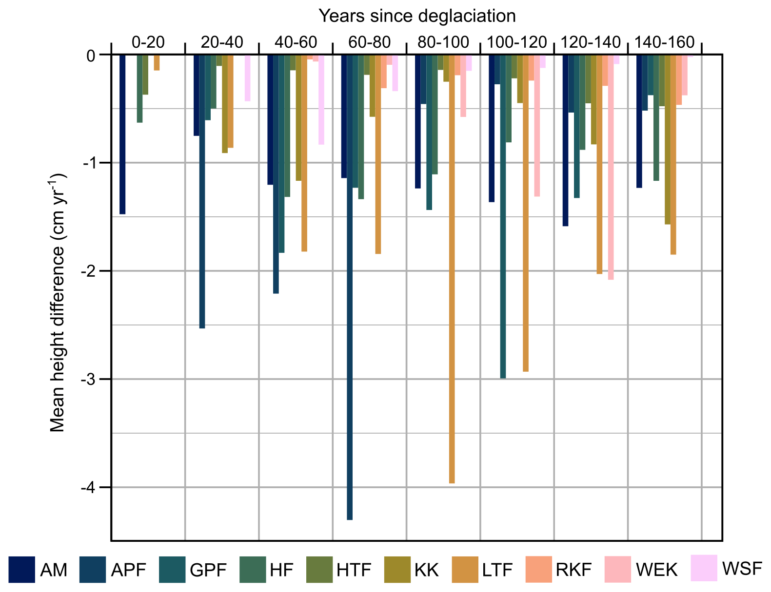
Figure 12 Mean annual height difference (based on the DoDs of the study areas covering time period 2; see Table 4 for specific DoDs) for different 20-year groups since deglaciation (relating to the mean year of the used DoD; colour map batlow10 from Crameri et al., 2020).

A comparison of the results of the analysis for the investigated moraine sections (Fig. 11) and the grid cells in the glacier forefields (Fig. 12) shows that in the former lower erosion rates are measured on moraine sections that were deglaciated at earlier points in time, whereas in the latter a consistent decrease in height differences with more years since deglaciation cannot be observed. The missing correlation in the grid-cell-based analysis can be explained by the simultaneous early deglaciation of the often highly active upper slopes and areas closer to the LIA glacier maximum which are, however, in general affected by only very little geomorphic activity. This shows that there is not a simple decrease in morphodynamics with increasing time since deglaciation, which indicates that the reason for higher erosion rates on moraine sections that deglaciated later is likely not given by the shorter time since deglaciation alone.

4.5.2 Slope angle

Correlation of the slope angle and geomorphic activity

The analysis of the slope angle and its influence on the geomorphic activity clearly shows that there is a correlation. In Fig. 13, classes of the slope angle (10^∘-classes) are plotted against the mean annual height difference in the DoD (volume difference per area covered by the raster cells of the respective slope angle class). It is visible that from a slope angle of 20–30^∘, the erosion rate increases until an angle of 60–70^∘ (single cells with more than 70^∘ were excluded). The highest erosion rates for the classes with the highest slope angle can be attributed to very high erosion on very steep but small areas. However, if the absolute sum of the erosion volumes is observed, i.e. without a standardization of the erosion volume to the area covered by the raster cells of the respective slope angle class (not shown here), most of the erosion can be detected on moraine slopes with slope angles of 30–40^∘ (38 %) and 40–50^∘ (30 %). In any case, only very little erosion takes place on moraine slopes with less than 30^∘.

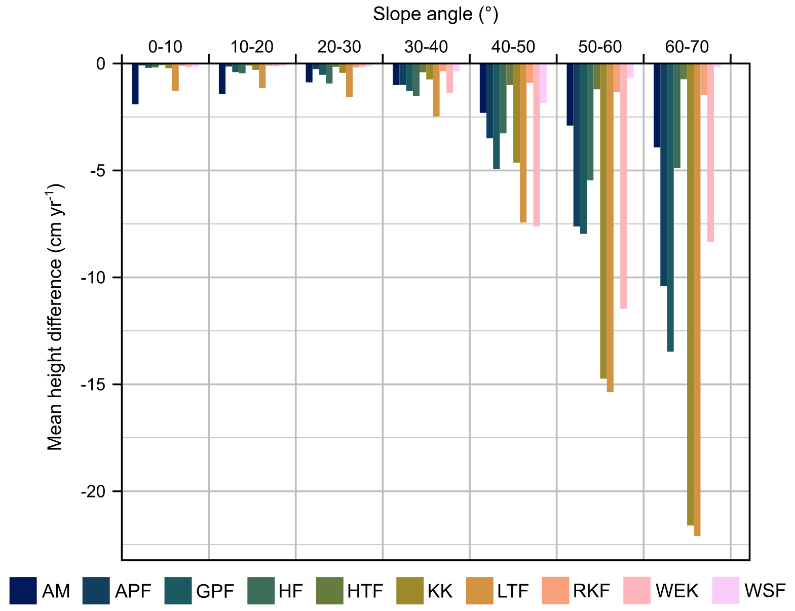
Figure 13 Mean annual height difference (based on the DoDs of the study areas covering time period 2; see Table 4 for specific DoDs) depending on the slope angle (colour map batlow10 from Crameri et al., 2020).

Dependence of the slope angle on the distance from the LIA maximum

Since the analysis above revealed that the erosion rate depends on the slope angle, we also analysed where within the glacier forefields particularly steep lateral moraine slopes can be found. For the Waxeggkees forefield, several cross profiles through the forefield show a decrease in slope angle with increasing distance from the location of the LIA maximum (see Fig. 14a and b). The same trend can be observed when looking at the mean slope angle at different positions between the upper end of the study area (see Sect. 2) and the maximum LIA extents in all investigated glacier forefields (Fig. 14c). This means that the mean slope angle increases in all analysed glacier forefields with increasing distance from the LIA glacier maximum within the study areas, albeit at different intensities and not always in a linear form. These variations can be explained by, e.g. bedrock areas that appear within the moraine tracts and have been excluded from the analysis. In any case, the slope angles are lower near the LIA maximum (0 %–10 %) than at a greater distance from the maximum, and this means that the potential for higher erosion rates also increases with increasing distance from the LIA glacier maximum.

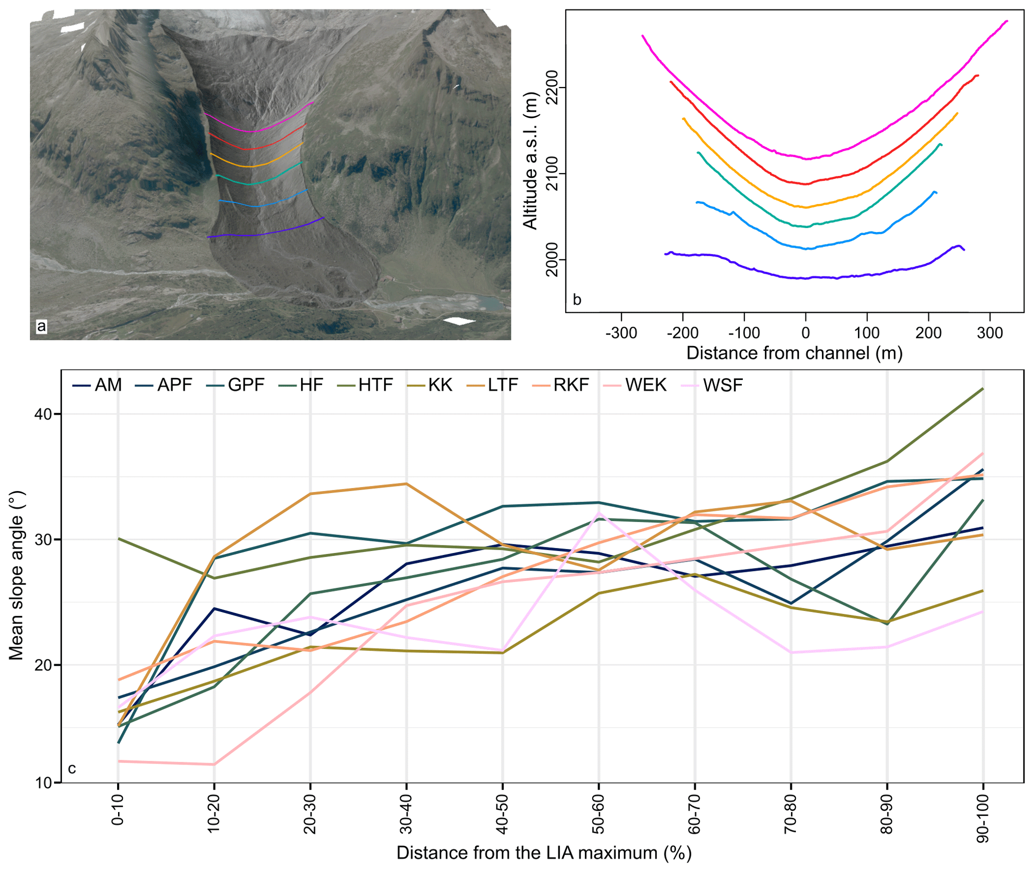
Figure 14 Slope angle depending on the distance from the LIA-maximum. (a) Oblique view of the Waxeggkees forefield with cross profiles in different distances to the LIA maximum (the source of 2010 aerial image is the State of Tyrol, Austria), shown in (b) against the altitude; (c) mean slope angles depending on the distance from the LIA maximum for all glacier forefields (100 % refers to the maximum distance from the LIA maximum within the respective study area, mean slope angle for each distance class is based on the newest DEM of the study areas; colour map batlow10 from Crameri et al., 2020).

Change in the slope angle over time

The findings shown above raise the question whether the decrease in the slope angle with increasing distance to the recent glacier tongue is a consequence of the longer time since deglaciation, since more time has already passed for adjustment, or of the genesis of the respective lateral moraines. For this purpose, the change in the slope angle over time was analysed for 20 upper slopes of the investigated moraine sections via a comparison of the slope angle in about 1950 (first available DEM) and 2018. In Fig. 15, the slope angle of ca. 1950 (x axis) is plotted against the difference in the slope angle between ca. 1950 and 2018 (in ^∘, y axis). Moreover, each moraine section is coloured by the magnitude of the erosion rate within the time period of the 1970s to the 2000s (red for >4 cm yr⁻¹, orange for 2–4 cm yr⁻¹, blue for 0–2 cm yr⁻¹). The plot shows that the moraine sections with the highest erosion rates (red) are characterized by an increase in the slope angle on the upper slopes, which is up to 6.6^∘, with one exception (GPF1). All but one of the moraine slopes with moderate erosion rates (orange) show a decrease in the slope angle, mostly of 0.2–2^∘, but the slope angle on one slope even decreased by 3.2^∘ (HF1). The moraine slopes with low activity (blue) show comparably little change in the slope angle due to very little sediment transfer. Overall, a clear decrease in the slope angles, following the idea of the paraglacial adjustment, is not detectable on the investigated upper slopes, especially not for the highly active moraine slopes, whose already steep upper slopes of 35–45^∘ steepened even more between ca. 1950 and 2018.

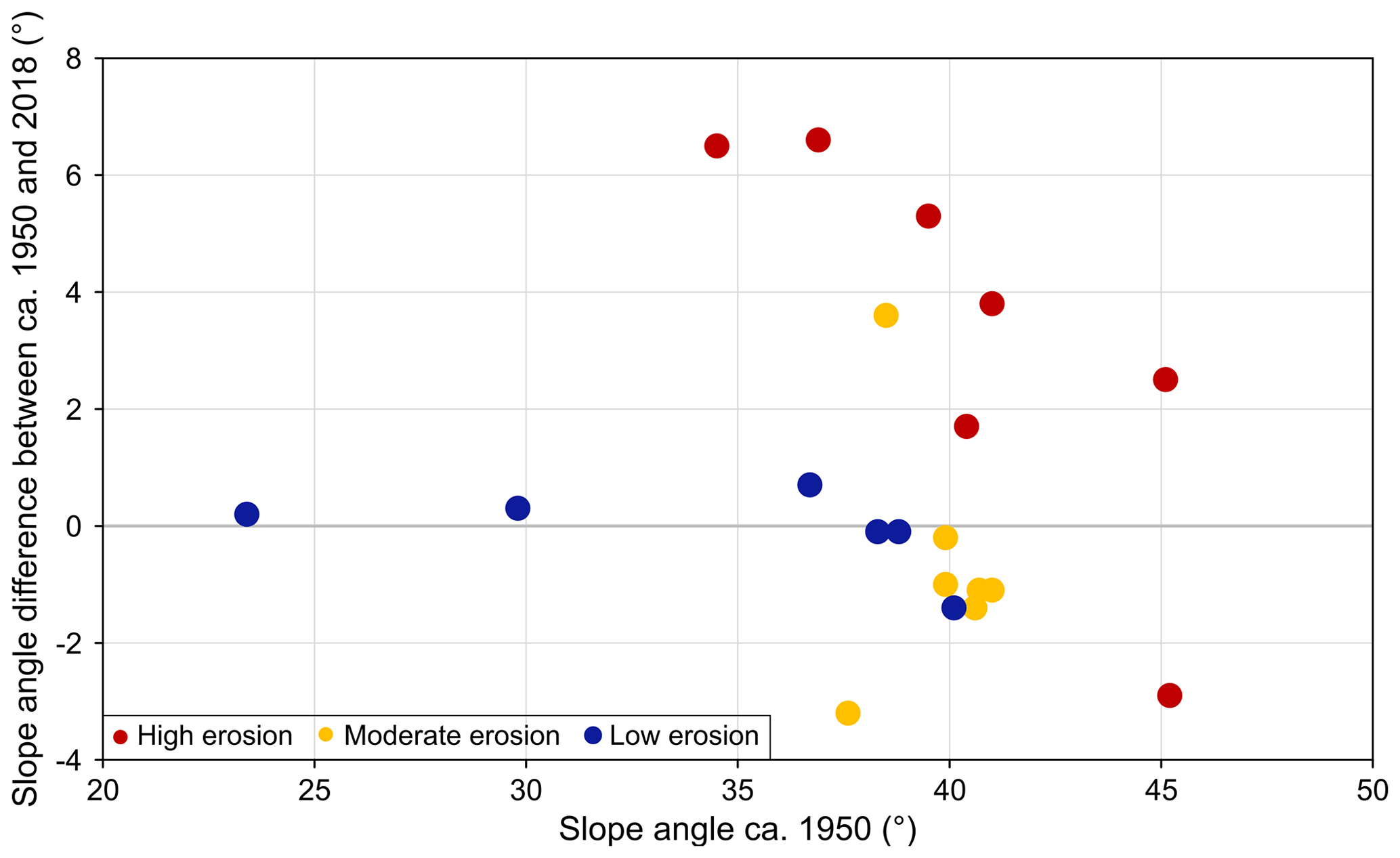
Figure 15 Change in the slope angle between ca. 1950 (1953/1954/1959/1960, depending on the DEM) and 2018 for the upper slopes of the investigated moraine sections. Colouring of the dots represents the mean erosion rates of the DoDs in time period 3 (see Table 4 for specific DoDs; erosion rate of 0–2 cm yr⁻¹ in blue, 2–4 cm yr⁻¹ in orange, and >4 cm yr⁻¹ red).

The result that the slope angles of lateral moraines do not decrease substantially over decades but presumably differ significantly already from the beginning of deglaciation is supported by old photographs from about 1900 showing the glacier forefields at a time when the glaciers still covered substantial parts of the LIA extent. Already at that time, the lateral moraines were less steep near the LIA maximum, but steep slopes deglaciated further upwards, e.g. visible for the Waxeggkees forefield in Fig. 16. Thus, the correlation between the slope angle and the distance from the LIA maximum, as shown above, is already visible at that time. This can be explained by the lower glacier ice thickness near the LIA maximum, which inhibits the forming of lateral moraines with high slope angles, unless certain conditions of the relief, such as larger bedrock areas, lead to a congestion of the ice masses also near the LIA maximum (e.g. observable in the Langtauferer forefield).

Table 6 Overview over the slope angle, erosion rate, recent activity, and years since deglaciation for all investigated moraine sections. Change in the slope angle is indicated if it was more than 1^∘ (median) between ca. 1950 and 2018. Change in the erosion rate is indicated if it exceeds 1.8 cm between the first and third period. Recent activity is based on time period 3 ($++$ for >4 cm yr⁻¹, + for 2–4 cm yr⁻¹ and 0 for 0–2 cm yr⁻¹).

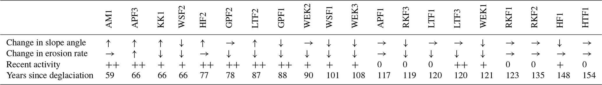
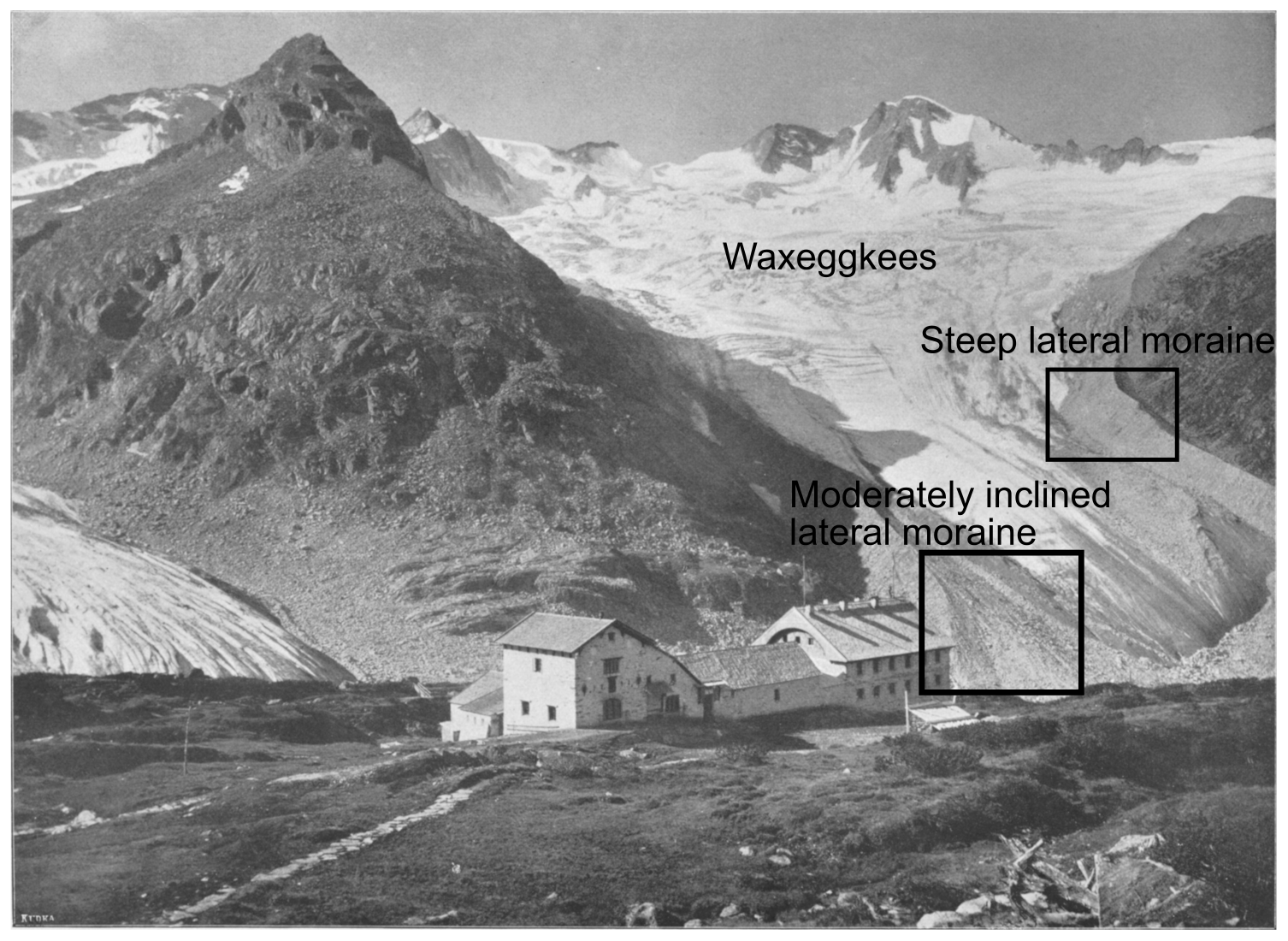
Figure 16 Photograph of the Waxeggkees showing lateral moraines with decreasing slope angle in the direction of the LIA maximum extent within the valley (Würthle & Sohn, Salzburg, in Platz and Rothpletz, 1903; courtesy of the Kulturarchiv Oberengadin).

4.6 Implications of the results for the paraglacial adjustment

The majority of the study areas show a decline in erosion rates over time from the 1950s to the 2000s. However, there are moraine slopes with an increase in or a stagnation of the erosion rate (see Table 6). Moreover, the erosion rates stay at a high level on some of the moraine sections. The fact that gullied slopes, which have already been deglaciated for 66 years, show still increasing erosion rates and that those that have been deglaciated for 120 years still show erosion rates of about 7 cm yr⁻¹ (LTF3), illustrates how long a stabilization on very steep and highly active slopes can take. The time since deglaciation for these gullied, very steep, and active slopes is not long enough yet to detect a stabilization. Since there are no slopes with deeply incised gullies in the study areas that feature even longer times since deglaciation, the future development of the steepest moraine sections cannot be predicted based on the available data.

Furthermore, a correlation between the development of the erosion rates and the time since deglaciation is unclear, as shown in Fig. 12 and Table 6 (comparison of change in erosion rate and years since deglaciation). For example, the most recently deglaciated moraine sections (59–66 years) developed diversely. Thus, the rapid paraglacial adjustment of gullied slopes after several decades, as postulated by Curry et al. (2006), Ballantyne (2002a), and Eichel et al. (2018), could not be generally proven, as several moraine sections did not show an increasing stabilization with ongoing time since deglaciation (e.g. HF1, LTF3, APF3). However, a tendency toward paraglacial adjustment over longer time periods than reported in the mentioned publications is indicated by our data.

It is probable that the differences between the results of this study and previous studies are due to the fact that the latter used space-for-time substitution instead of an observation over longer time periods. Using space-for-time substitution for the study areas of this work would have generated similar results regarding the erosion rates because the slopes closer to the LIA maximum (older with respect to the time since deglaciation) show smaller erosion rates than the ones at a larger distance (see the comparison of recent activity and years since deglaciation in Table 6). However, it should be noted that different initial conditions of the slopes at the time of deglaciation are not reflected with the use of space-for-time substitution, as also described in Wojcik et al. (2021) for the investigation of vegetation succession. Yet, the initial conditions can have a substantial influence on the morphodynamics. As our results showed, the slope angle is an especially crucial factor determining the morphodynamics on a moraine slope. When comparing moraine sections in different distances to the LIA maximum, as is done when using space-for-time substitution, slopes are compared that probably did not have comparable slope angles at the time of deglaciation due to the glacier ice mass distribution. Thus, it is clear that less inclined slopes with a shorter distance from the LIA maximum also exhibit lower erosion rates and show earlier signs of stabilization and vegetation succession. However, this is not necessarily or not solely due to a longer time since deglaciation. This shows the importance of the analysis of multitemporal DoDs in several glacier forefields in order to properly investigate trends of morphodynamics.

These results show that high slope angles are a necessary precondition for high morphodynamics. Further influence factors can determine if a steep lateral moraine indeed shows high erosion rates and, e.g. heavy gullying. The factors altitude, slope undercutting by channels, climate, and geology were investigated in Betz-Nutz (2021) and did not show a clear influence on the morphodynamics on the lateral moraines. A stabilizing effect of vegetation growth due to biogeomorphic interactions is assumed, but the vegetation succession depends on the altitude, moisture availability, etc. (Betz-Nutz, 2021; Schumann et al., 2016; Eichel et al., 2016). Factors such as the local substrate, the potential for headward retreat, and non-local factors, such as the size of the catchment, should be investigated further.

5 Conclusion

The following conclusions can be drawn from our analyses.

1. The use of data covering several decades, which is possible with the processing of historical aerial images, makes a space-for-time substitution dispensable. Instead of comparing different moraine sections regarding their different time since deglaciation, it is possible to analyse morphodynamics over time on the same moraine section. This enables new insights and reveals the true complexity of the development of lateral moraine slopes in glacier forefields. It shows, e.g. that the course of development of moraine sections that deglaciated a longer time ago does not necessarily provide information about the future development of younger moraine sections.

2. Melting dead ice is an important factor to consider when analysing the development of glacier forefields and especially moraine slopes. This melting ice can lead to an ongoing destabilization of the slopes and thus decelerate the process of stabilization.

3. The highest morphodynamics occur on very steep moraine slopes with deeply incised gullies. On these slopes, high erosion rates could be detected over many decades, often with ongoing gully incision and headward retreat. Slopes that did not experience a heavy gully erosion and incision seem to show more signs of stabilization.

4. The time since deglaciation alone does not explain the pattern of active or less active areas within the glacier forefields.

5. The slope angle seems to be the crucial factor determining the geomorphic activity of moraine slopes. Only on slopes with at least 30^∘ slope angle can high morphodynamics be detected. The distribution of the glacier ice mass during the LIA maximum and historical photographs both suggest that the slope angle on lateral moraines was lower with a smaller distance to the LIA maximum from the beginning of deglaciation onward.