Patterns and rates of soil movement and shallow failures across several small watersheds on the Seward Peninsula, Alaska

Thawing permafrost can alter topography, ecosystems, and sediment and carbon fluxes, but predicting landscape evolution of permafrost-influenced watersheds in response to warming and/or hydrological changes remains an unsolved challenge. Sediment flux and slope instability in sloping saturated soils have been commonly predicted from topographic metrics (e.g., slope, drainage area). In addition to topographic factors, cohesion imparted by soil and vegetation and melting ground ice may also control spatial trends in slope stability, but the distribution of ground ice is poorly constrained and hard to predict. To address whether slope stability and surface displacements follow topographic-based predictions, we document recent drivers of permafrost sediment flux present on a landscape in western Alaska that include creep, solifluction, gullying, and catastrophic hillslope failures ranging in size from a few meters to tens of meters, and we find evidence of rapid and substantial landscape change on an annual timescale. We quantify the timing and rate of surface movements using a multi-pronged, multi-scalar dataset including aerial surveys, interannual GPS surveys, synthetic aperture radar interferometry (InSAR), and climate data. Despite clear visual evidence of downslope soil transport of solifluction lobes, we find that the interannual downslope surface displacement of these features does not outpace downslope displacement of soil in locations where lobes are absent (downslope movement means: 7 cm yr⁻¹ for lobes over 2 years vs. 10 cm yr⁻¹ in landscape positions without lobes over 1 year). Annual displacements do not appear related to slope, drainage area, or modeled total solar radiation but are likely related to soil thickness, and volumetric sediment fluxes are high compared to temperate landscapes of comparable bedrock lithology. Time series of InSAR displacements show accelerated movement in late summer, associated with intense rainfall and/or deep thaw. While mapped slope failures do cluster at slope–area thresholds, a simple slope stability model driven with hydraulic conductivities representative of throughflow in mineral and organic soil drastically overpredicts the occurrence of slope failures. This mismatch implies permafrost hillslopes have unaccounted-for cohesion and/or throughflow pathways, perhaps modulated by vegetation, which stabilize slopes against high rainfall. Our results highlight the breadth and complexity of soil transport processes in Arctic landscapes and demonstrate the utility of using a range of synergistic data collection methods to observe multiple scales of landscape change, which can aid in predicting periglacial landscape evolution.

1 Introduction

In Arctic, sub-Arctic, and Antarctic regions, the presence of permafrost and seasonal thaw leads to a range of soil transport processes strongly influenced by the thermal dynamics of the landscape (Harris and Lewkowicz, 2000; Matsuoka, 2001; Millar, 2013). Water and sediment fluxes are also influenced by the presence of excess near-surface ground ice (Li et al., 2021; Mithan et al., 2021) and limited subsurface infiltration of surface waters due to the presence of impermeable permafrost and seasonally frozen ground (Walvoord and Kurylyk, 2016). As with non-permafrost regions, rates, mechanics, and timing of downslope soil movement on hillslopes play a fundamental role in landscape evolution (Lavé and Burbank, 2004; Roering et al., 2007); the transport and storage of soil organic carbon (Yoo et al., 2006); the delivery of sediment, carbon, and nutrients to streams (Berhe et al., 2018); and the stability of infrastructure (Hjort et al., 2022). Despite decades of research on patterns and rates of soil movement in periglacial environments (Carson and Kirkby, 1972; Matsuoka, 2001; French, 2018), the geomorphological and permafrost research communities lack process-based transport formulations to parameterize landscape evolution models applicable to permafrost-dominated regions.

Increasing research focus on the Arctic and permafrost regions has drawn attention to the large quantities of soil organic carbon stored in northern high-latitude soils (Hugelius et al., 2014; Olefeldt et al., 2016; Shelef et al., 2017). Numerous studies have highlighted the magnitude of carbon release that may be associated with thaw of frozen carbon (Schuur et al., 2015), though these estimates have large uncertainties. Recent estimates of possible carbon release due to catastrophic erosional events suggest that overlooking these rapid processes may drastically underestimate carbon release from hillslopes under future warming (Turetsky et al., 2020). However, these estimates carry uncertainties that arise both from limited quantification of carbon stocks and very limited understanding of how climate and landscape dynamics interact in permafrost settings to control the magnitude, location, and rate of landscape change and carbon release.

Predicting slope failures in any soil-mantled landscape generally involves estimating a baseline force balance on the hillslope and tracking any temporal change in stresses in the soil. This force balance is controlled by the topography and soil thickness (Montgomery and Dietrich, 1994), which modulate slope, shear stress, and hillslope hydrology. The hydrology in turn controls the saturation state and pore pressure acting within the soil (Montgomery and Dietrich, 1994; Lu and Likos, 2006). Therefore, any change to the rate and volume of water supplied to a soil-mantled hillslope will change the stress balance. An increase in high-latitude slope failures (Balser et al., 2014; Lewkowicz and Way, 2019) has occurred as summers get both warmer and wetter (Hu et al., 2015; Douglas et al., 2020). This poses a conundrum for understanding the main driver of slope stability in permafrost: is summer thaw happening deeper and faster, resulting in thaw-consolidation-driven failures on ice-rich planes? Or do intense summer rainfall events on ever-deepening active layers alter the force balance and trigger landslides? Or are both combining to the destabilization of hillslopes? Most studies of modern permafrost slope stability involve statistical correlations between historical failure sites and topographic or climatic metrics (Lewkowicz and Harris, 2005; Balser et al., 2014; Lewkowicz and Way, 2019). However, since future Arctic climate change has no modern precedent, empirical studies may be inherently limited in future applicability. Therefore, understanding the mechanisms and topographic controls on hillslope processes is crucial for making process-based predictions of Arctic sediment and carbon balances as 21st century warming proceeds.

In this study, we present multiyear observations of recent topographic change and sediment transport in a relatively steep watershed (10–25^∘ slopes) on the Seward Peninsula, AK. Our site is located within the discontinuous permafrost zone, and over the course of study (2017–2019) the site experienced both warmer-than-average and wetter-than-average summers, making it a sensitive, ideal location to study how permafrost thaw modulates sediment flux and slope stability. We use differential GPS (DGPS), synthetic aperture radar interferometry (InSAR), orthoimagery, and digital elevation models (DEMs) collected via uncrewed aircraft system (UAS) to track topographic changes in the landscape. We evaluate spatial and temporal trends as functions of topography and hydrology to assess the transferability of slope-stability predictions formulated in temperate landscapes.

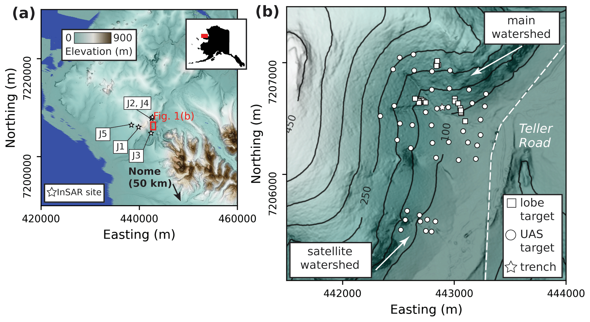
Figure 1 Overview of regional setting (a), with location within Alaska, and site (b). Star symbols in (a) indicate locations of InSAR-derived displacement observations. In (b), squares denote differential GPS survey targets for lobe features, and circles denote targets for uncrewed aerial survey (UAS) calibration points. Star is location of deep (>1 m) trench. Location of Teller Road is shown as a white dashed line. Contour lines are 50 m intervals for elevation data. Elevation data are meters above sea level derived from ArcticDEM. Northing and easting coordinates UTM zone 3N.

2 Study area

Our study area is on the western Seward Peninsula (65^∘ N) in western Alaska (Fig. 1) and underlain by the Precambrian Nome Group, comprised of chlorite and marble schists, and the Precambrian Slate of the York region, which contains metamorphosed interbedded dolomitic and argillaceous bedrock. Both units are in places intruded by coarse-grained gabbros and diabases (Sainsbury, 1972), expressed as rocky unvegetated areas on the surface. Unglaciated hillslopes support a rocky, thin (up to 1–2 m) soil mantle that is commonly organized into turf-banked solifluction lobes (defined as isolated, tongue-shaped features with relatively smooth upper surfaces) and sweeping solifluction terraces (steps or benches with straight fronts) (Harris, 1988; Kaufman et al., 1989). Last Glacial Maximum (LGM) glaciation was limited to the Kigluaik Mountains to the southeast, but earlier Pleistocene glaciation may have been more extensive and reached some portions of the study area (Kaufman et al., 2011). The study region is bordered by the Imuruk Basin to the northeast and Port Clarence to the north, both of which drain into the Bering Sea to the west, which underwent large changes in sea level during the last glacial period (Elias et al., 1996; Lozhkin et al., 2011). The study watershed, located along the Teller Road, lies near the drainage divide between Canyon Creek, which drains to the Imuruk Basin to the east, and McAdam Creek, which drains to the Bering Sea to the west.

The study area is underlain by discontinuous permafrost, and the mean annual air temperature for the region from 1980–2015 was −6 ^∘C with a positive trend of 0.06 ${}^{\circ }\mathrm{C}{\mathrm{yr}}^{-\mathrm{1}}$ (Thornton et al., 2016; Jafarov et al., 2018). Over the same period, total average rain and snow precipitation were ∼400 and 300 mm yr⁻¹, respectively; snow precipitation has declined while rain precipitation has increased (Jafarov et al., 2018).

3 Methods

We collected field and remotely sensed data from several small watersheds along the Teller Road near mile point 47, and hence we refer to the site as “Teller 47”. We collected differential GPS data in June and July 2017, July 2018, and August 2019, and during the 2018 and 2019 campaigns imagery was collected via uncrewed aircraft system (UAS). Our August 2019 field season began 5 d after an unusually intense rainstorm between 1–3 August; detailed field observations were made at the site to document the geomorphic and hydrologic consequences of the storm. A meteorological station located within the study area (442937.59 E, 7206428.18 N UTM 3N; 67 m above sea level; Busey et al., 2021) that records data every half hour recorded 77 mm of rain in 65 h, with a peak rainfall intensity of 9.6 mm h⁻¹ on 2 August; these data were supplemented with historical climate data from the Nome Regional Airport (Alaska Climate Research Center Data Portal, 2022). We also mapped subseasonal surface movements across the landscape using InSAR (interferometric synthetic aperture radar) from satellite data from 2014 to 2019. We synthesized these datasets to connect discrete and continuous measurements of surface displacement to climate and topographic drivers.

3.1 Differential GPS

In June 2017, 20 survey markers were placed in four clusters on solifluction lobe treads and downslope of lobe fronts to track annual movement both on and around lobe treads (Fig. 1b). The markers are white plastic rectangles measuring 40 cm × 70 cm and were secured with two rebar rods in the center of the marker. The bottom of the rebar was hammered to a depth of up to 50 cm, and the remaining protruding rebar at the surface was capped with a rebar cap. When measuring the height of the target at the rebar, we measured the height of the rebar caps and subtracted the height of the rebar to calculate the position of the target flush to the tundra surface. On the northernmost, south-facing slope, targets were distributed across three lobes with dimensions of ∼40 m in the upslope direction and ∼20 m in the cross slope. On the east-facing hillslope located between the two tributary branches of the main drainage, we placed a fourth cluster of 10 targets across a series of arcuate features with torn vegetation and exposed soils upslope and apparent bunching of tundra and soils downslope.

We used a Trimble R10 integrated GNSS System (base and rover) to re-survey the four corners and tops of the two rebar poles for all survey markers for each year. We collected GNSS observations at each point for 30 s. The base was positioned at the same location each year for the annual survey. The system's effective accuracy has both intrinsic uncertainty (8 mm horizontal and 15 mm vertical) and depends on a survey's greatest distance from a point to the base (for our surveys, 925 m, or 0.925 network real-time kinematics (RTK) parts per million (ppm), a unit of uncertainty specific to the model) such that our surveys have accuracies of ∼9 mm in the horizontal and ∼16 mm in the vertical. We surveyed the solifluction lobe markers for 3 years: when the targets were first deployed June 2017, July 2018, and August 2019. This produced 2 years' worth of interannual displacement measurements. To compare interannual movement we averaged the four XY positions at each marker corner to produce a single coordinate for a target each year with an uncertainty (calculated via standard error) of ±1.8 cm horizontal and ±3.2 cm vertical. We then calculated the distance between each years' target-averaged point in both the horizontal and vertical to determine annual displacement. Survey points were corrected using the Online Positioning User Service (OPUS; https://www.ngs.noaa.gov/OPUS/, last access: June 2020) and adjusted (e.g., corrected for base receiver height above ground) in Trimble Business Center software.

To investigate potential controls of interannual displacement measured by DGPS, we compared displacement magnitudes to topographic attributes that were likely to influence movement. We calculated the upslope contributing area at each survey point as a proxy for saturation. We resampled the 2 m ArcticDEM digital elevation model of the site to 10 m using bilinear interpolation to minimize the effect of microtopography on topographic metrics and calculated topographic slope with RichDEM (Barnes and Bovy, 2022) and modeled total incoming solar radiation as watt hours per square meter using the Solar Radiation tool in ArcMap of the area around each survey point.

3.2 Field mapping and UAS imagery

In July 2018 we used a DJI Phantom 4 Pro uncrewed aircraft system (UAS) to collect >6800 high-resolution aerial photos of the lower portion of the watershed. At the time of the UAS survey, we laid out 41 25 cm×25 cm tile ground control points (GCPs) secured with one rebar rod in the center. The rebar tops were surveyed with differential GPS, and these coordinates were used to construct and validate the orthomosaic. We also surveyed the gridded UAS markers in August 2019, rendering only a single interannual displacement measurement.

We used Agisoft Metashape photogrammetry software to construct a georeferenced orthomosaic image of a portion (0.68 km²) of the watershed with a final horizontal resolution of ∼1 cm. We selected a subset of 75 % of surveyed GPS points to align the model and visually checked that the remaining 25 % of markers' centers aligned with the GPS points.

We manually delineated the perimeters of failures visible in the UAS imagery and created shapefile polygons. The failures were identified by the exposure of bare mineral soils due to disruption of the overlying tundra vegetation. We used the shapefiles to analyze the topographic distribution and sizes of the failures.

In August 2019, we surveyed the Teller 47 watershed with GPS points, photographed changes, and measured depth to permafrost using tile probes. We made particular note of new slope failures and evidence of incision into the tundra mat. We also collected an additional ∼300 georeferenced UAS images of slope instability features using the same equipment as in 2018. We performed an initial orthomosaicking of the 2019 images based on the georeferencing of the images, after which resulting orthomosaics were georeferenced to the 2019 imagery based on identifiable control points in both images such as shrubs, rocks, trees, and other presumably stable features. Because we targeted 2019 photography for failures, a complete orthomosaic of the 2018 survey area was not collected. Any failures mapped in the 2019 imagery that were also present in the 2018 imagery were manually removed from the 2019 inventory. For areas not covered by orthomosaics but were photographed via UAS, we mapped failures on individually georeferenced and orthomosaicked images.

We mapped the regions lacking near-surface permafrost based on field probing and coring, topographic properties, and vegetation distributions at the study site. In unfrozen hollow fills and lobes, the absence of permafrost was confirmed by the excavation of opportunistic pits and a trench up to 2 m in depth. These observations were used to map permafrost-free locations and inform estimates of the extent of thawed areas along drainages based on both the presence of dense shrubs and trees and the presence of grasses instead of tundra, a robust pattern observed at both our site and with geophysical observations at a nearby site (Uhlemann et al., 2021). A rough estimate of the extent of permafrost-free areas in the study area is presented in Fig. 2a. Permafrost depth probing sites were selected opportunistically as we traversed the watershed, and thus the permafrost-free extent mapped in Fig. 2a is approximate.

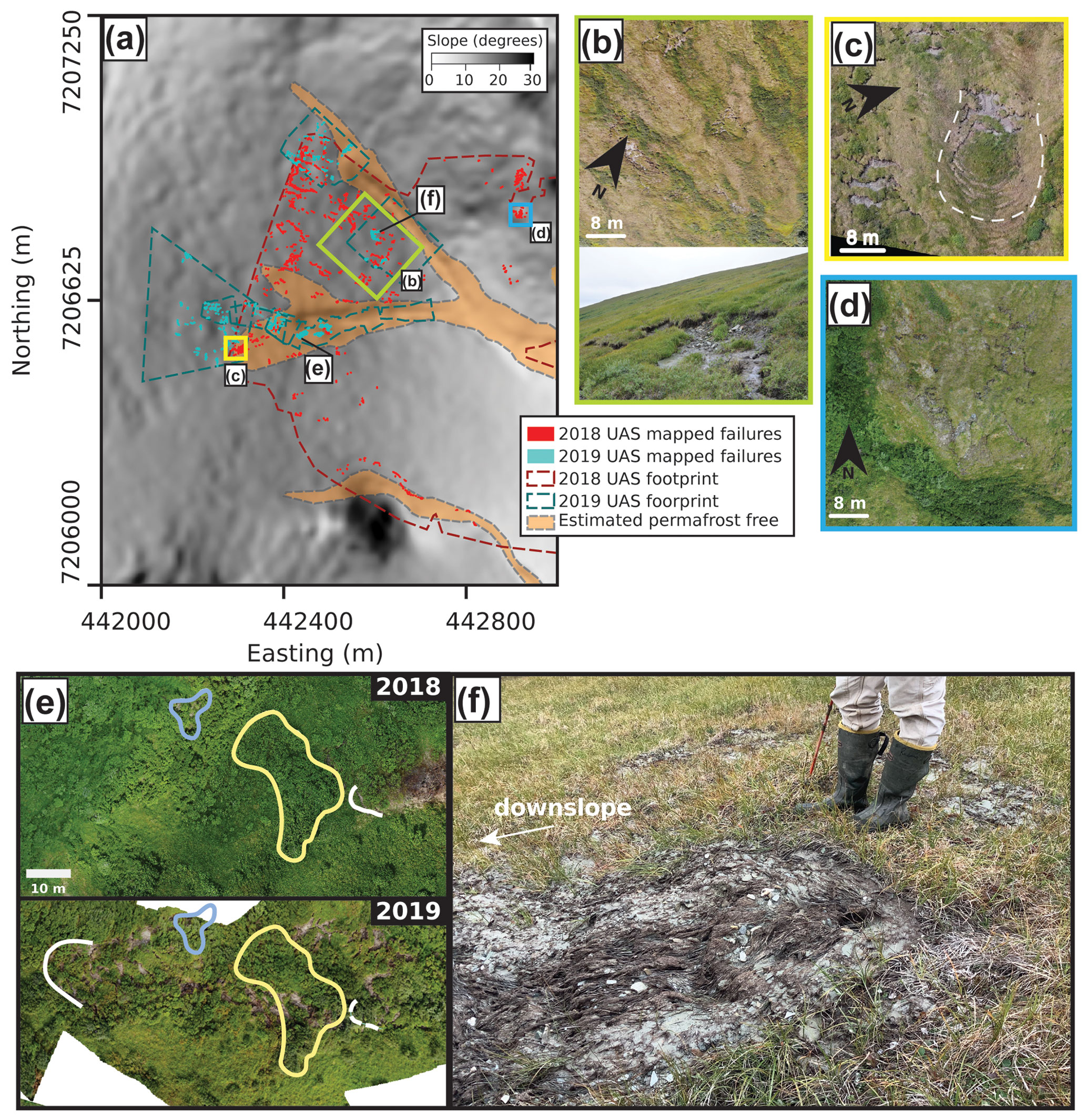
Figure 2 Landforms and slope failures at the Teller 47 watershed. (a) Slopeshade of ArcticDEM topography model overlain with mapped failures in 2018 (red) and 2019 (cyan). (b) Many small arcuate failures occur on the steeper slopes of the watershed. (c) The area around the two channels exhibited detachment of the tundra mat from the underlying mineral soil in arcuate shapes (white dashed line). Separation of the tundra at the head of a failure results in rumpled tundra at the toe. (d) In an area of more convergent topography, overland flow incised through the tundra mat and exposed mineral soil. (e) Gully head retreat of ∼70 m between July 2018 and August 2019; each year's gully head shown with a solid white line, with the 2018 location shown as dashed lines in 2019. The translation of a group of shrubs downslope is demonstrated with their position outlined in yellow in 2018 and the same location, now with exposed soil, shown in 2019; the blue outline is another incipient failure. (f) Mud ejection feature with ∼10 cm diameter vent.

3.3 InSAR

We mapped subseasonal surface movements across the landscape using InSAR (interferometric synthetic aperture radar) at a resolution of 100 m. While these observations cannot resolve fine-scale processes such as the shallow failures in Fig. 2, we studied them to identify their association with rainfall events on the hillslope scale. To this end, we processed Sentinel-1 observations (Torres et al., 2012) between early June and mid-September 2017–2019 at a resolution of 100 m. The Sentinel-1 observations from path 15, frame 377 were available at 12 d intervals from an easterly look direction (101^∘ azimuth angle, 38^∘ incidence angle). To determine the slope and aspect of the underlying topography on a scale that matched that of the radar data, we resampled the ArcticDEM topography model with bilinear interpolation to 15 m and smoothed the resulting topography with a Gaussian filter (σ=1.5 pixels).

The line-of-sight (LOS) motion measured by InSAR will contain contributions from downslope and surface-perpendicular movements at any given location. The easterly look direction implies that downslope and perpendicular movements added destructively over the southwest-facing Teller 47 hillslope, compounded by poor resolution (foreshortening). Unfortunately, a dense time series of Sentinel-1 observations from the opposite look direction is not available.

To estimate the line-of-sight movements, we used a short baseline (SBAS) approach (Berardino et al., 2002). We first formed the interferograms at a resolution of 100 m by multilooking with a rectangular boxcar filter (13 range × 5 azimuth samples). Owing to the rapid loss of coherence, we only processed interferograms with temporal separations of up to 24 d, and the interferograms were then unwrapped using the SNAPHU package, which is based on a network optimization approach (Chen and Zebker, 2001). After geocoding using the TanDEM-X 90 m DEM, we referenced the interferometric phases at bedrock outcrops, which we assumed to be stable. We then estimated the movement time series from the interferogram stack by weighted least squares, with the weights determined by the Cramér–Rao coherence-derived estimate of the phase variance (Zwieback and Meyer, 2021). The standard error of the Sentinel-1 displacement estimates in northwestern Alaska was estimated at approximately 1 cm by Zwieback and Meyer (2021). We consistently adopt the sign convention that positive movements correspond to increasing LOS distance between the satellite and the surface.

To constrain the subseasonal movements of hillslopes in the study area, we focused on five locations close to the Teller 47 site. The reason we did not analyze the movements at the Teller 47 site are the unfavorable viewing geometry: steep southeast-facing slope with destructive interference of downslope and surface-perpendicular motion and low coherence due to foreshortening. Instead, we selected five nearby sites of predominantly west-facing aspect (determined using the TanDEM-X DEM) with similar surficial characteristics (Fig. S1 in the Supplement). We checked these locations with favorable viewing geometry manually to rule out phase unwrapping errors, which manifest as regions where the displacement estimates have an offset.

3.4 Slope stability

3.4.1 Topographic controls on failure locations

To determine whether our mapped slope failures occurred at particular slope–area thresholds, we extracted the average value of the 15 m slope and 2 m drainage area rasters for each failure polygon as well as for the entire area covered by the UAS survey. To more clearly differentiate failure locations across different geomorphic regimes, we binned the total area of both the hillslope and failure polygons in logarithmic bins (i.e., powers of 10) for drainage area between 10¹–10⁴ m² as well as slope bins between 7–25^∘. Casting failure locations in slope–area space assists in determining the dominant process regime (e.g., hillslope versus fluvial; Montgomery and Dietrich, 1994; Tucker and Bras, 1998).

3.4.2 Infinite slope model of stability

We compared our slope failure inventory to an implementation of SHALSTAB, a topographically derived landslide susceptibility model (Montgomery and Dietrich, 1994). The model uses upslope contributing area and soil transmissivity as a proxy for pore-water pressure generated by precipitation of a given rate. We applied the model to our field site under the conditions of an intense rainfall event on 2 August 2019, during which rain fell at a maximum rate of ∼50 mm d⁻¹. We calculated rasters for slope on a resampled 10 m DEM using the GDAL and RichDEM packages (Barnes and Bovy, 2022), and we calculated drainage area on the original 2 m ArcticDEM raster with a D-infinity algorithm (Tarboton, 1997) using the Flow Accumulation tool in ArcMap for the study area. We assumed a soil thickness of 1 m, equivalent to the active layer depth we observed in August, assuming the permafrost table below represented an impermeable layer similar to bedrock in the original implementation of the model. We used a bulk saturated hydraulic conductivity (K_sat) of 2.2 m d⁻¹, using estimates made for a nearby site (Jafarov et al., 2018) and assuming $\mathrm{1}/\mathrm{3}$ of the active layer was an organic horizon and $\mathrm{2}/\mathrm{3}$ of the active layer was mineral soil, to calculate the ratio of throughflow q to soil transmissivity t. This metric produces a map of relative wetness in the landscape, where high $q/t$ represents areas with throughflow rates much higher than the soil can transmit indicating a greater likelihood of failure.

4 Results

4.1 Field observations

4.1.1 Observations of slope failures

We noted new slope failures and areas of tundra disturbance in August 2019 not visible in the 2018 UAS imagery (Fig. 2). One major failure occurred on the planar, south-facing slope in between the two first-order drainages (Fig. 2b). Here, the tundra mat and some underlying mineral soil (up to 10 cm) had been detached, forming an arcuate area of exposed cobble-rich soil upslope and a “rumpled” mat of tundra downslope. Along the edges of this failure, water was flowing both atop the vegetation mat as well as incising deeply (>1 m) into the mineral soil on the margins of the failure and flowing into the main channelized drainage network downslope.

Another major form of tundra disturbance was apparent piping of water from below the soil to the surface of the tundra in an eruption of soil, cobbles, and water (Fig. 2f). The site of the pipe emergence was strewn with clods of sedge, fine-grained soil, and rock fragments up to 10 cm diameter up to 5 m away from the pipe. Downslope of the pipe, sediment tens of centimeters in thickness buried green undisturbed tundra, implying that sediment was transported in large volumes from the pipe tens of meters downslope.

Other failure styles we observed included small (1–3 m across) semi-arcuate detachments of the tundra and up to ∼10 cm of underlying soil, revealing crescent-shaped exposed mineral soil (Fig. 2b). There appeared to be a range of ages to these failures, revealed by the appearance of the exposed mineral soil surface. Surfaces that were comprised almost entirely of fine-grained material, which sometimes still bore slickenline-like striations in the direction of failure, appeared to be recent; we suspect these delicate striation features would have been destroyed had they occurred prior to the 2 August rainstorm. Other failure surfaces contained more pebbles and cobbles, implying removal of fines via slopewash indicating these surfaces at least pre-dated the 2 August rainstorm.

The crescent-shaped failures appeared upslope of and in association with lobe treads. In 2019, we observed buckled tundra vegetation and shrubs that had overridden intact vegetation forming a rumpled and rounded elevated nose front (Fig. 2c). These features were most common on the middle east-facing slope, but morphologically similar features, highlighted by shrub growth along the lobe fronts, occur on the south-facing slope in areas where permafrost is no longer present. Where failure occurred on lobe treads, portions of the tundra mat were translated downslope but remained intact. On the east-facing slope for flows we visually determined to be somewhat recently active, the average downslope distance between the soil exposing detachments and the lobe front was 45 ± 15 m (mean and standard deviation), with average widths of 19 ± 5 m and areas of 67 ± 376 m², based on measurements of digital mapping (see code and data repository).

Another failure style was the expansion outward and upslope of the gullies at our site. Based on 2018 and 2019 UAS imagery and 2019 field surveys, the head of the southeast-flowing gully migrated upslope about 70 m (Fig. 2d). We also noted extensive tundra disturbance within ∼30 m of the area surrounding the gully head as well as the banks 100 m downslope. The east banks of the adjacent watershed also had failure surfaces noted in 2018 imagery that expanded as noted in 2019 field surveys.

We visually mapped ∼1200 individual failures from 2018 orthoimagery, amounting to ∼600 m² of area, or 0.09 % of the area of the watershed covered by our orthoimagery (0.67 km²) (Fig. 2a). These failures averaged 0.5 m² (±1.1 standard deviation) in area and 0.48 m (±0.43 standard deviation) in width measured normal to the downslope direction (see code and data repository). The maximum area and width mapped were 20.6 m² and 6.6 m, respectively. Failures were concentrated on the southeast-facing planar slope between the two first-order streams. Other failures occurred on the east-facing slope that was characterized by tussock tundra and water tracks (Evans et al., 2020), whose flow lines indicated divergent flow paths. On the southwest-facing slope, which contained rockier soil and no water tracks, failures were restricted to an area of convergent topography.

We mapped 205 new failures on hillslopes in the 2019 orthomosaics covering 0.04 km² of the study area. On the hillslopes, the average area (0.87 ± 1.67 m²) was slightly larger and downslope width (0.51 ± 0.43 m) was similar to the failures mapped in the 2018 imagery (see code and data repository). New failures along the axis of the southern tributary to the main drainage mapped via orthomosaics (n=32) were even larger with an average area of 4.3 (±3.3) m² and average width of 1.6 (±0.95) m. The maximum area and width were 13.3 m² and 4.3 m, respectively. We mapped an additional 121 failures from individual orthomosaicked images.

In 2017 we encountered frozen soils at the head of the southernmost drainage at the site; however later in the summer during the 2019 field effort, no frozen material was encountered within 2 m of the surface of the exposed hollow face, suggesting the frozen material encountered in 2017 was seasonally frozen or that rapid loss of permafrost occurred following the failure. In 2019, opportunistic digging into failure faces along the other drainages at the site only exposed unfrozen deposits. The trench into the lobe (Fig. 1b) also indicated that the absence of permafrost extended northward from the main drainage and was associated with dense 2–3 m high shrubs along the front of lobes and grasses on the flat lobe platforms. Soil coring further upslope on the south-facing slope indicated that presence of permafrost was heterogenous with frozen soils absent in large 2–3 m high lobes. Based on our limited coring, however, the full extent of permafrost and non-permafrost regions was not delineated.

4.1.2 Differential GPS interannual displacement measurements

Mean annual horizontal and vertical change of lobe targets from the 2-year period of 2017–2019 was 7.1 ± 4.3 cm (1 SD) and 8.7 ± 5.6 cm, respectively (Fig. 3) (with uncertainty deriving from the 1.8 cm uncertainty of DGPS measurements) (see supplemental data; raw data hosted within data repository assets). Lobe targets moved an average of 8.0 ± 3.3 cm in the horizontal direction and 8.0 ± 6.1 cm in the vertical direction from 2017–2018, and 6.3 ± 5.7 cm and 9.4 ± 7.6 cm in the horizontal and vertical directions, respectively, from 2018–2019. We recorded three upwards interannual vertical movements (inflation). In general, lobe targets that had higher magnitudes of movement in 2017–2018 also had large movement magnitudes in 2018–2019 (Fig. S2). We did not observe a systematic pattern of movement with position on lobes across the landscape. On two lobate features, targets closest to the lobe front moved faster than targets upslope on the tread (Fig. 3b), but this pattern was not observed at other locations where a lobe had more than one survey target (see Supplement).

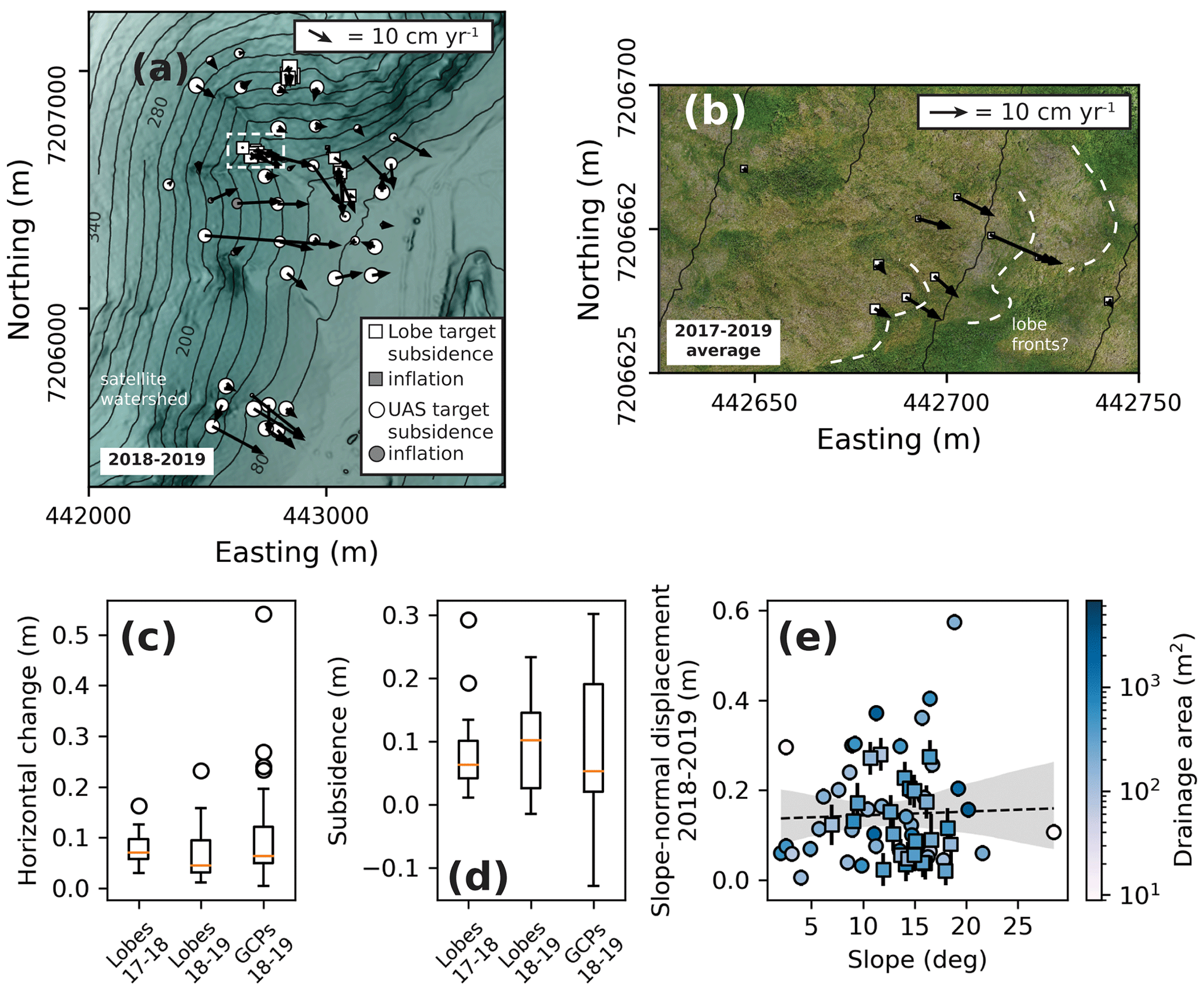
Figure 3 (a) Map of 2018–2019 displacement vectors including horizontal displacements (arrows) and elevation changes (squares for lobes, circles for UAS targets). Arrow and symbol size scales with magnitude. Elevation data are the same as Fig. 1b. Figure 3b location is shown as a dashed white box. (b) Zoom-in to orthoimage derived from UAS imagery to vectors associated with lobate features with speculative lobe fronts delineated in a white dashed line. Arrow and square size represents average annual displacement vectors across the 2 years (2017–2019). (c) Boxplot showing horizontal change for each measurement type and year. Orange lines within boxes are medians; white circles are outlier data. (d) Subsidence magnitudes; elevation increases are negative values. (e) Scatterplot of lobe marker (squares) and UAS target (circles) displacement versus slope, with symbols colored by the drainage area at that position. Regression line includes a 95 % confidence interval.

A t test for independent samples applied to 2018–2019 displacements (Virtanen et al., 2020) found no significant difference between magnitudes of movement of lobe targets and magnitudes of movement of GCPs laid out in a grid (see Supplement). Gridded targets moved an average of 10.2 ± 10.6 and 6.3 ± 10.1 cm in the x and z directions, respectively, but there was a larger spread in displacement magnitudes than for lobe targets. Some gridded targets moved up to 5× as much as other targets. Unlike lobe movements, which tended to cluster between 5–10 cm yr⁻¹, some gridded target movement magnitudes were >25 cm yr⁻¹ (Fig. 3c). We recorded several negative vertical displacements but no negative horizontal displacements.

Both lobe and grid targets had smaller-than-average displacements on the south-facing, steep, rocky slope in the north of the watershed where the presence of permafrost may be more sporadic (Fig. 3a). At the base of all hillslopes and across the relatively flat alluvial plain near the drainage outlet, displacements were also low. Locations upslope of the gully heads exhibited a wide range of displacements; these positions correspond to the region of many smaller tears in the tundra mat of varying ages, as discussed above. The satellite watershed in the SW of the survey region, which we have observed to be actively gullying, has moderate to high displacement magnitudes (Fig. 3a).

Lobe total (horizontal plus vertical) displacement from 2017–2019 has no discernible correlation with slope, drainage area, or modeled solar radiation, and nor do movements from the individual years 2017–2018 and 2018–2019 (Figs. 3e and S2). The gridded targets demonstrate a weakly positive relationship between slope angle and displacement, but there is considerable scatter in the magnitude of displacements. There is also no clear relationship between drainage area or modeled solar radiation and displacement magnitude.

4.2 InSAR

We show the cumulative and differential displacements averaged over five hillslope sites (J1–J5; see Fig. 1a) normalized to a 90 d period beginning in early summer and ending in early autumn for years 2017–2019 (Fig. 4a and b). Cumulative displacement in 2019 exceeded that of previous years by up to a factor of 2. For four out of five locations, the InSAR estimates show a notable acceleration in early August 2019 that lasted for at least 1 month. For J4, the acceleration started before the 4 August 2019, acquisition; for J1 and J2 it started afterwards. In previous years there was either no apparent late-season acceleration (2017) or it set in mid-August (2018).

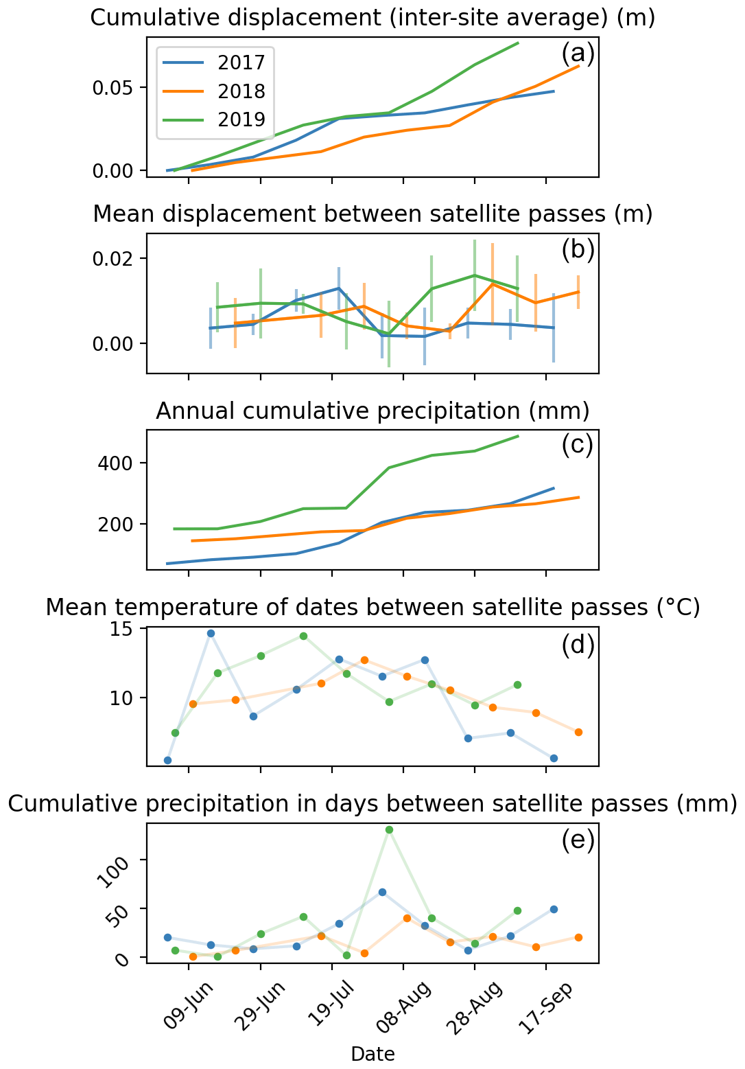
Figure 4 InSAR displacements versus climate variables during the corresponding satellite passes: (a) cumulative displacement; (b) differential movement (vertical error bars are 1 standard deviation across the five sites); (c) cumulative precipitation during the satellite recording time; (d) 12 d rolling average temperature between satellite passes; (e) 12 d cumulative rainfall between satellite passes.

We compare the observed displacements to the nearest long-term climate data collection site at Nome Airport (Alaska Climate Research Center Data Portal, 2022). The higher cumulative displacement in 2019 compared to the previous 2 years mirrors cumulative rainfall recorded at the station. By the season's end, cumulative rainfall in 2017 and 2018 was approximately half of cumulative rainfall in 2019, and those years experienced about half as much cumulative displacement as 2019 (Fig. 4). We derived values for the mean temperatures (Fig. 4d) and cumulative rainfall (Fig. 4e) of the 12 d in between satellite passes to ascertain the relationship between movement and meteorological variables; except for the rainstorm of August 2019, there is no apparent pattern.

4.3 Slope stability

4.3.1 Topographic controls on failure locations

The location of mapped slope failures in the subset of the watershed covered by orthoimagery in 2018 and 2019 cluster at slope–area thresholds (Fig. 5). Most failures occurred between slopes of 14–20^∘ and drainage areas between 0.1–1.2×10³ m². Normalizing for the proportion of the mapped landscape that falls into each slope–area bin, more failures occur in the higher drainage areas ($>\mathrm{0.5}\times {\mathrm{10}}^{\mathrm{3}}$ m²) on slopes of 14–20^∘. At both exceptionally steep slopes (>22^∘) and at exceptionally high drainage areas ($>\mathrm{1.5}\times {\mathrm{10}}^{\mathrm{3}}$ m²), relatively high proportions of the hillslope falling within this slope–area bin experience failures; indeed failures seem to follow contours of steepness (the product of slope and the square root of drainage area) (Fig. 6).

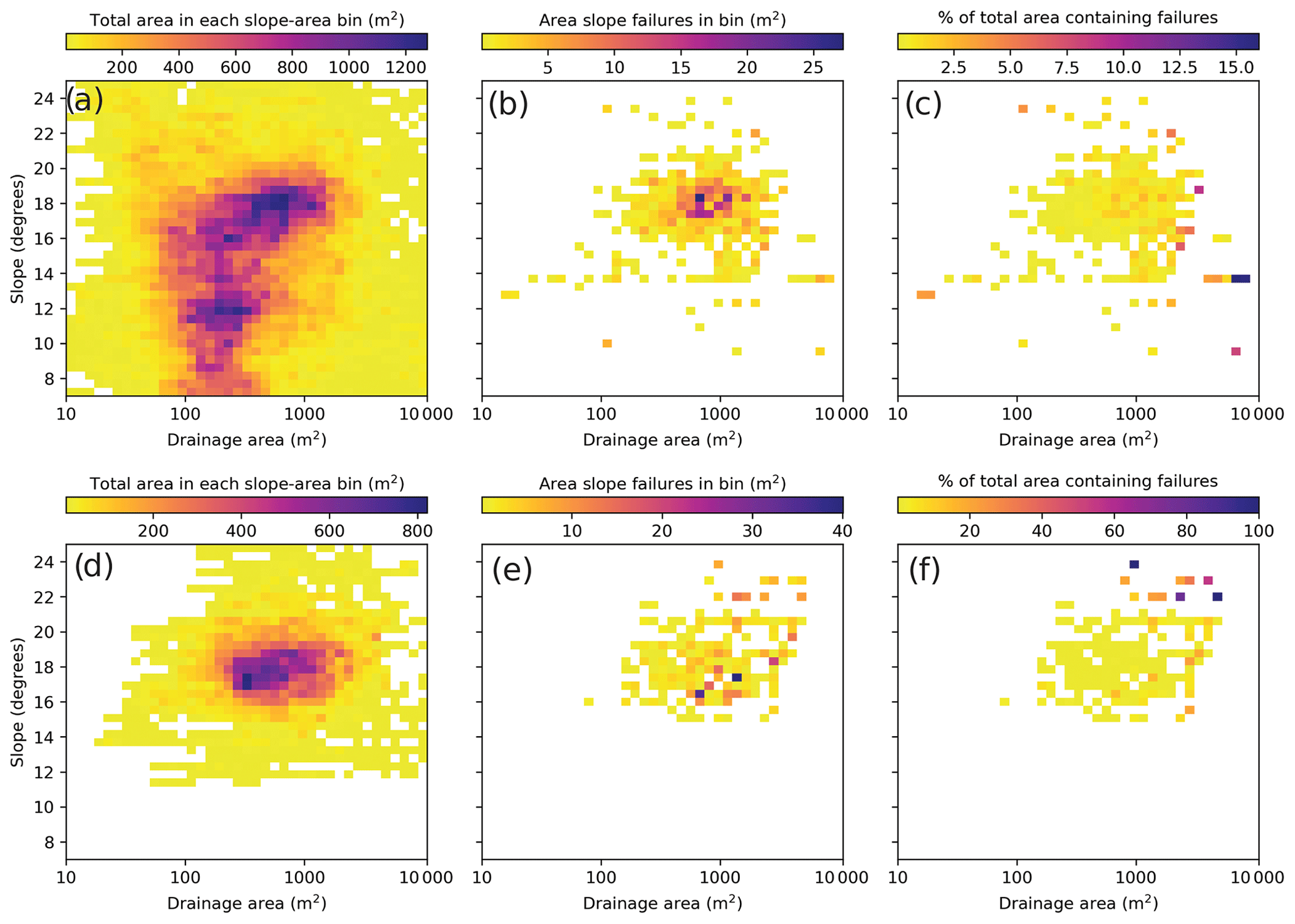
Figure 5 Mapped slope failure locations in slope–area space versus total area covered by UAS surveys in 2018 (a–c) and 2019 (d–f). (a) Total area of the DEM covered by the 2018 UAS survey that falls into each slope–area bin. (b) The summed areas of failure polygons whose centroids fall within a slope–area bin. (c) The proportion of failure areas to the total area covered by the UAV (the ratio of b to a). Panels (d–f) are the same but for the 2019 UAV survey footprint. In (f), note that some failures' areas were larger than the total area of the slope–area bin in which its centroid fell, resulting in high failure rates for that bin.

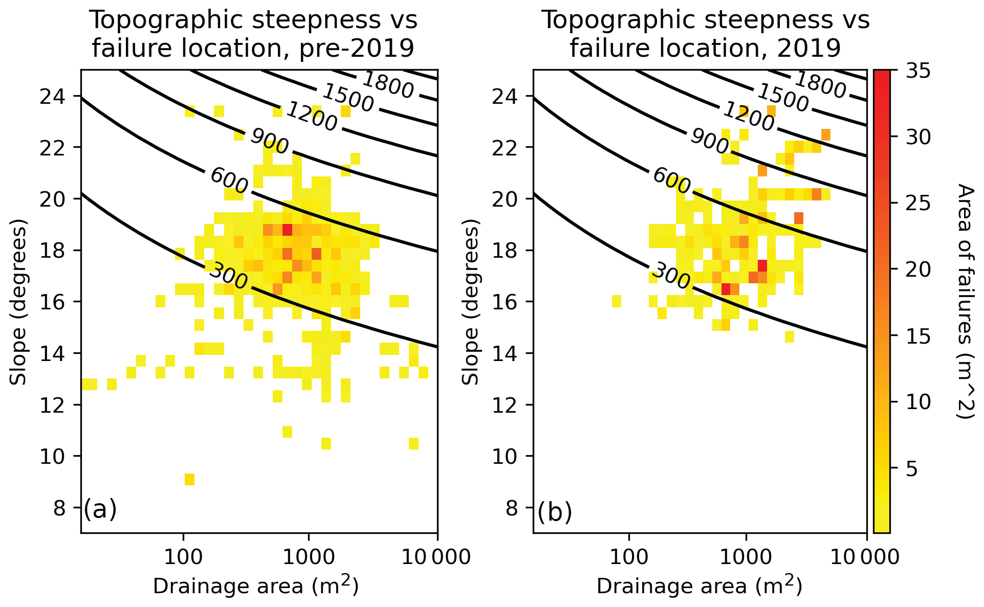
Figure 6 Mapped failures (a) before and (b) after the August 2019 rainstorm and survey plotted in slope–area space with contours demonstrating topographic steepness (the product of slope and the square root of drainage area). Colors demonstrate areal extent of failures that fall into each slope–area bin versus the entire area represented by the UAS survey region.

4.3.2 Infinite slope model of stability

We calculated the critical rainfall rate (q_cr, mm d⁻¹) needed to induce driving forces to exactly balance resisting forces (factor of safety (FS)=1) (Montgomery and Dietrich, 1994) (Fig. 7a). We show results for a range of precipitations that reflect historical rainstorms as observed at the Nome Airport: the annual peak daily rainfall since 1900 has ranged between 10–60 mm d⁻¹. Thus, we consider landscape positions for which q_cr<10 mm d⁻¹ to represent unconditionally unstable positions (failure of the soil column is predicted to occur without the addition of water), q_cr between 10–60 mm d⁻¹ to be conditionally stable (failure dependent on water volume added), and q_cr>60 mm d⁻¹ to be unconditionally stable (failure not predicted at saturation).

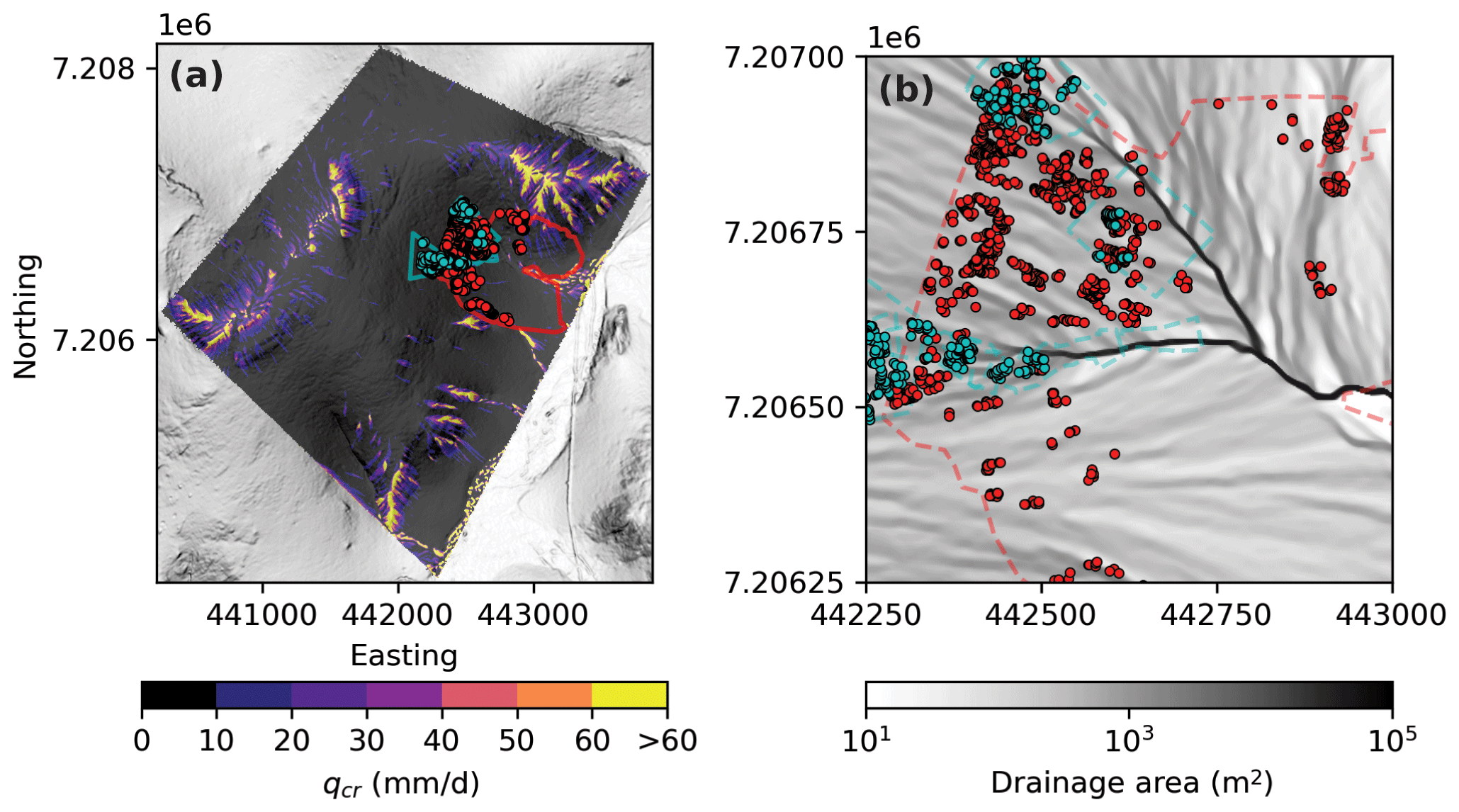
Figure 7 (a) Map of entire SHALSTAB model domain with color contours demonstrating critical rainfall (q_cr) necessary to instigate failure. Note most of the model domain is predicted to be unconditionally unstable given our parameters (see text). UAS survey area and mapped failures in 2018 (red) and 2019 (cyan) shown. Background slopeshade generated from ArcticDEM as described in the text. (b) Drainage area versus mapped failures. Dashed lines are UAS survey areas as in Fig. 2a.

A striking feature of the SHALSTAB model output is that a majority of the hillslope is expected to experience excess throughflow and thus failure given the conditions of the 2 August rainstorm where q=50 mm d⁻¹ (Fig. 7a). Although most of the noted major slope failures in 2019 do occur in areas with modeled excess throughflow (true positives), a vast portion of the east-facing hillslopes were also expected to have excess throughflow, but the tundra was observed to be intact with no recent failures noted (false positives).

5 Discussion

5.1 Rates and patterns of hillslope sediment flux

5.1.1 Geomorphic controls

We suspect that soil thickness plays a role in explaining the spread of interannual displacement measurements, although we did not systematically measure soil thickness. The locations with small displacement for both grid and lobe targets were typically on steeper slopes with patchier vegetation and cobble-rich soil exposed at the surface (Fig. 3a). Targets with thin, rocky soils also tended to be steeper sloping, contributing to the scatter of slope versus displacement. In contrast, targets on steep slopes with thick soils had large magnitudes of downslope displacement. Locations with finer and thicker soil are expected to host more ground ice in the transition zone in the upper permafrost, promoting soil shear at depth as permafrost thaws (Kirkby, 1995; Lewkowicz and Clarke, 1998; Shur et al., 2005).

Previous studies have found that solifluction lobes tend to move faster than the surrounding soil (Harris et al., 2008; Ballantyne, 2013; Eichel et al., 2020). This contrasts with our results, in which soil transport rates are similar between lobes and surrounding hillslope locations (Fig. 3c and Supplement). There are several possibilities to explain this discrepancy. First, lobes likely move faster because they are thicker than the surrounding topography (Glade et al., 2021). We lack constraints on presence or depth of permafrost and soil at survey sites over time, and it is possible that the difference in thickness between lobes and non-lobes is minimal, leading to similar transport rates. Second, it is well known that soil velocities vary substantially within a single solifluction lobe, with the highest velocities in the middle and near-zero velocities at the front (Benedict, 1970; Eichel et al., 2020). This pattern is likely due to the dynamics of lobe movement, in which lobes roll over themselves at the front similarly to a fluid front flowing down a plane (Glade et al., 2021). Because we placed our targets at a variety of sub-lobe positions, it is possible that our displacement data reflect the noise of the within-lobe variability in deformation and thus are difficult to relate directly to topographic metrics. Finally, vegetation is thought to be an important control on solifluction lobe deformation; different species prefer to grow on lobes, often concentrated at the front of the lobe where drainage is greatest (Price, 1974; Benedict, 1976; Eichel et al., 2017). While we did not conduct a comprehensive vegetation survey, all lobe fronts at the site have been colonized by shrubs, and it is possible that over time preferential plant colonization at lobe fronts has slowed down solifluction lobes relative to the surrounding topography.

5.1.2 Parameterizing thawed soil movement for predictions and modeling

The average displacement of 5 cm yr⁻¹ measured on lobes and surrounding topography at the Teller 47 watershed is slightly faster than most annual surface displacements of solifluction lobes in a recent compilation of field observations (Glade et al., 2021) and corresponds more closely with solifluction rates described in Matsuoka (2001) in warmer and typically alpine environments.

Our measurements from an active permafrost hillslope offer an opportunity to consider how hillslope sediment flux might be parameterized in a landscape evolution model. Landscape evolution models for periglacial landscapes parameterize sediment transport as dependent on the thermal state of the soil and thus interpret an “effective diffusivity” based on the volume of sediment moved during thaw (Bovy et al., 2016). Assuming an exponential velocity profile with depth observed in most periglacial hillslope settings (Glade et al., 2021), DGPS-derived surface velocities observed in the field over the 2017–2019 period can be extrapolated to velocity profiles at depth (Eq. 1) and transformed into an annual sediment flux per unit width q_s (Eq. 2) with the following formulations (Johnstone and Hilley, 2014):

$$\begin{array}{}\text{(1)}& {\displaystyle }V\left(h\right)=V_{\mathrm{0}}{e}^{\frac{-h}{d_c}}\text{(2)}& {\displaystyle }{q}_{\mathrm{s}}=V_{\mathrm{0}}{d}_c\left(\mathrm{1}-e^{\frac{-H}{d_c}}\right),\end{array}$$

where V is the velocity of soil at a given depth, V₀ is the surface velocity, h is the surface normal depth at a point in the soil column, H is the total depth of soil over which to integrate the flux, and d_c is a scaling depth whose value sets the shape of the velocity profile. Using a thaw depth of 100 cm and surface velocity of 5 cm yr⁻¹ on a slope of 15^∘, modeled on our DGPS observations, we estimated volumetric sediment flux with depth–velocity profiles that resemble field- and lab-derived profiles (Lewkowicz and Clarke, 1998; Glade et al., 2021). Although we had no field data to determine velocity profiles with depth, compilations from solifluction movement (Glade et al., 2021) imply global solifluction profiles are best fit with scaling depths d_c between 5 and 20 cm (Fig. 8). This range of d_c results in estimated volumetric sediment fluxes of 25–100 cm² yr⁻¹.

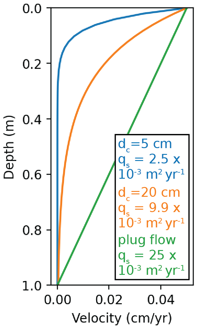
Figure 8 Representative velocity profiles of solifluction and associated volumetric sediment fluxes (q_s) for an active layer of thickness 1 m, such as observed at the Teller 47 site. For exponentially decaying profiles as observed in sites compiled by Glade et al. (2021), the depth at which V(h)=0 varies between 20 and 80 cm. For plug flow, modeled off the observations of Lewkowicz and Clarke (1998), velocity decays linearly with depth and thus represents higher volumetric sediment fluxes.

Our study highlights the variety of complex processes driving periglacial slope instability. Soil, especially when subjected to freeze–thaw and temporally changing saturation conditions, likely behaves as a complex soft material, sometimes behaving as a solid and sometimes behaving as a fluid (Jerolmack and Daniels, 2019; Glade et al., 2021). For this reason, we strongly caution against the use of simple hillslope diffusion transport laws (e.g., Dietrich et al., 2003) in periglacial landscape evolution models. However, because most hillslope studies report estimates of diffusivity values as opposed to volumetric flux, for the purposes of comparison we use our surface velocity data to estimate hillslope diffusivities at our site. Assuming that the surface velocity is controlled by a diffusion-like process, where V₀=kS, where k is a measure of hillslope transport efficiency and S is the topographic slope (Johnstone and Hilley, 2014), we find estimated diffusivity constants between 94–372 cm² yr⁻¹ for portions of the hillslope where the soil thickness would span the entire depth of the modeled thickness (≥1 m).

The low end of these estimated diffusivities is higher than >80 % of diffusivities compiled by Hurst et al. (2013) and igneous and metamorphic landscapes by Richardson et al. (2019) in middle-latitude landscapes. These values imply high hillslope diffusivities in this permafrost landscape compared to temperate landscape measurements, in line with modeled assumptions of high shear rates in thawing permafrost (Kirkby, 1995; Bovy et al., 2016). Note that our estimates of volumetric flux and diffusivities come from the DGPS measurements and do not include failures; thus they likely underestimate the annual flux at our site. Further, this annual flux estimate is conservative because it assumes little movement with depth (d_c=5 cm), while plug-like flow from shear along saturated zones at the base of the active layer can drive deep-seated movement in late summer (Lewkowicz and Clarke, 1998; Matsuoka, 2001; Shur et al., 2005). While we lack in situ observations of the late-season acceleration in the InSAR time series, the acceleration is consistent with plug-like flow (Harris et al., 2011). We also caution that our instantaneous measurements of modern, active movement are difficult to compare against morphometric-derived diffusion constants and other long-term records of sediment flux; in addition, volumetric fluxes will be lower where soils are thin because there is less soil to transport at depth (see Fig. 3a). However, this analysis suggests that soil transport rates in periglacial settings can be more rapid than those in temperate regions.

Based on the mismatch between observed and modeled slope failures, using topographic metrics like slope and drainage area may not be sufficient to predict slope failure on short temporal and spatial scales due to the stochasticity and heterogeneity of such systems. However, these metrics may still be useful for driving longer-term landscape evolution models for steady processes, notorious collapsers of stochasticity. Observations of warming-induced shear in field and modeled permafrost soils (Carson and Kirkby, 1972; Harris et al., 1997; Lewkowicz and Clarke, 1998; Matsuoka, 2001) have led to models of permafrost landscapes that link soil transport efficiency to the cumulative thaw depth over a summer, maximizing soil diffusivity at MAT at or around 0 ^∘C (Kirkby, 1995; Anderson, 2002; Anderson et al., 2013; Andersen et al., 2015; Bovy et al., 2016). However, these models are agnostic toward both the rate at which warming proceeds and the direction of temperature change (warm to cold vs. cold to warm). More work is needed to understand whether current “snapshots” of surface displacements are representative of either long-term sediment flux or warming-induced disturbance.

5.2 Patterns and styles of abrupt erosion and slope failures

5.2.1 Observed erosion and slope failures

Field observations suggest that slope failures occurred at a range of depths. The saturated state of the soil during August 2019 fieldwork made excavation and identification of failure planes difficult. However, the tears in the tundra vegetation mat and associated below-ground roots that exposed mineral soils upslope of the compressional lobes likely occurred at some depth within the mineral soil profile. Given high hydraulic transmissivity and low bulk density of the tundra vegetation mat, it seems unlikely the tundra alone was detaching and failing; instead, flow of soil beneath the vegetation likely pulled the vegetation along with it at the lobe front, as evidenced by the bulked and rumpled vegetation in the nose and tore the upslope vegetation far from stable portion of the hill upslope. Within and directly above the hollows, deeper failures (1–2 m) may be triggered by destabilization of the hillslope by gullying and incision in the stream channels. These failures occur both above and lateral to the gullies, and multiple episodes of failure pre- and post-2019 suggest this instability may be propagating upslope through regions of the hillslope lacking permafrost.

The tendency for failures to occur in higher drainage areas for a given slope (Figs. 5 and 6) implies that saturation and throughflow likely play a role in destabilizing that slope position. Since inflection points in slope–area space are thought to indicate changes in process between diffusive hillslope processes and advective fluvial processes at a saturation threshold (Tucker and Bras, 1998; Clubb et al., 2016), these failures probably represent hillslope positions that failed at saturation when throughflow was high.

In contrast, the failures mapped on low slopes, but high drainage areas (14^∘ and 1.5×10³ m²) represent a different failure regime. In the field, we observed soil piping that led to water and sediment transport downslope in the form of overland flow. In addition to soil piping, overland flow paths that previously routed through the tundra exhibited new incision into the underlying mineral soil and deposited sediment downslope. Surface and shallow subsurface water flows on the tundra are known as water tracks (Mcnamara et al., 1999; Trochim et al., 2016), which are present at our site in the form of vegetation contrasts and subtle concavities on hillslopes. In 2019, we observed both channelized surface flows through the tundra mat as well as numerous instances in which overland flow in water tracks had breached the tundra mat and root layer and was incising into the mineral soil below. This implies some incision or saturation threshold was crossed, allowing water to incise through the otherwise strong, permeable tundra mat. Once that incision begins, the saturated fine-grained soil is easily eroded.

5.2.2 Model predictions and implications

The SHALSTAB model overestimates the regions of the Teller 47 watershed prone to failure when using values for the saturated hydraulic conductivity (K_sat) of the organic horizon (∼6.0 m d⁻¹) and mineral soil (0.06 m d⁻¹) from previous hydrologic models for a hillslope hydrology model of a nearby watershed (Jafarov et al., 2018). However, the SHALSTAB model requires a minimum of 100–200 m d⁻¹ for most hillslope positions to achieve a factor of safety of unity (driving and resisting forces exactly balanced). For the bulk K_sat of the soil profile to reflect the relative stability of the hillslope (since all points on the hillslope did not fail), the mineral soil may have a higher K_sat, but it is more likely that the rainfall runoff moving through this landscape is not infiltrating into the mineral soil as true throughflow and instead flows through both the organic soil layers and peaty tundra mat. Cohesion, particularly in the root zone, would also contribute to higher-than-modeled slope stability.

Since water tracks can support surface flows on permafrost hillslopes without necessarily interacting with the underlying mineral soil (Trochim et al., 2016; Evans et al., 2020), these water flow paths are good mechanisms to explain the overprediction of slope failures at higher drainage areas. Though the topographic signature of water tracks is subtle on the landscape at the 2 m scale, slight variations in convergent and divergent topography emerge in our wetness model, which correspond to water track flow paths. While some of these areas do indeed contain mapped failures (Fig. 2d), clearly much of this area did not fail during the 2 August rainstorm (Fig. 7b). Moreover, based on historical rainfall data (Alaska Climate Research Center Data Portal, 2022), the landscape experienced storms with sufficient rainfall to initiate failure in these parts of the landscape as well, and yet no failures are observed. This implies that the tundra mat and water tracks allow excess throughflow to work its way to the channel network without initiating a channel.

These observations show that while slope failures and gully locations are controlled by topography, both the permeability of the tundra mat and the cohesion imparted by its roots (Gyssels et al., 2005) are likely important mediators of rainfall infiltration and slope stability that complicate topographic-based predictions. Both subsurface flow rate and root cohesion are important elements of the force balance on slopes and require extensive field characterization (Parker et al., 2016; Hales, 2018). To improve predictions of both pore-pressure-induced slope failures and shear stress-driven gullying, observations of partitioning of throughflow into the permeable tundra mat versus the impermeable mineral soil are needed, as well as estimates of the shear strength that the tundra mat imparts on the surface of the hillslope to inhibit incision below some threshold (Tucker and Bras, 1998; Istanbulluoglu and Bras, 2005).

5.3 Ground ice thaw versus summer rainfall as driver of disturbance

What are the relative contributions of precipitation and ground ice thaw to the observed landscape disturbances at our site? The apparent pipe flow, excavation, and ejection of mineral soil and rocks under the tundra observed in 2019 (see Fig. 2e) suggest hydraulic heads above ground surface. On Ellesmere Island in 2005, rapid and deep thaw led to high porewater pressures creating similar mud ejection features (Lewkowicz, 2007). Conditions in which hydraulic head is elevated above the ground surface could be driven by rapid thaw as proposed by Lewkowicz (2007) or by intense rainfall as occurred at the site on 2 August. Another dramatic process, the gully head retreat that occurred between July 2018 and August 2019, appears unrelated, at least directly, to permafrost thaw as we did not observe permafrost in the upper meter of soil surrounding the major drainages (Fig. 2).

Attributing remotely sensed surface displacement to either rainfall or warming remains elusive. The InSAR-observed late-season acceleration in surface displacement in 2019 may be explained by subsidence and downslope motion triggered by the melting of excess ice near or at the top of the permafrost (Zwieback and Meyer, 2021), as well as by increased downslope movement promoted by wetter conditions. We note apparent acceleration of surface displacement after late-season rainfall in both 2018 and 2019, whereas in 2017, early-season warming may have led to accelerated displacement ∼24 d later. In contrast, the above-average temperatures in early July 2019 do not correspond to additional displacement. Whereas the temperature trends for warmer months (early June through early September) are similar over the 2017–2019 periods, the total rainfall varies more considerably, from a low of 150 mm in 2018 to a high of 250 mm in 2019; cumulative displacement thus more closely mirrors cumulative rainfall for 2017–2019.

If the present-day form of soil-mantled permafrost hillslopes is adjusted to transport sediment under the colder Neoglacial of the past 5 kyr (Hunt et al., 2013; Kaufman et al., 2016) and indeed most of the Quaternary, either deepened active layers and/or higher rainfall amounts could promote slope instability. On soil-mantled sloping surfaces, thawed, saturated soils are prone to slope failure due to increased pore pressure from saturation and/or reduced cohesion from lack of ground ice. On landscape positions currently occupied by water tracks, thaw of ground ice would promote subsidence and subsequently wetter and thus warmer ground temperatures (Evans et al., 2020), and increased overland flow due to high rainfall would promote shear stresses necessary to overcome any incision inhibition imparted by vegetation.

Recent work modeling slope stability of thawing permafrost hillslopes found that high concentrations of ground ice near to the potential failure plane had more influence over the slope's stability compared to high ground ice volume in general or the pace at which thawing proceeded (Mithan et al., 2021). In this model, however, the only source of excess pore-water pressures was the thawing ice lenses themselves, with no representation of upslope hydrology channeling either meltwater from upslope ice lenses or any precipitation-derived moisture. These models also produced failure planes close to the base of the active layer to simulate the active layer detachments observed in the central Brooks Range (Balser et al., 2014), potentially deeper and morphologically different than the failures observed at our site. Understanding whether ground ice thaw or summer rainfall drives erosion is thus important for predicting landscape response to projected climate change in the Arctic.

Are ongoing climate trends in the Arctic making the landscape more susceptible to erosion? In addition to continued warming of the Arctic in the Anthropocene, hydroclimate changes may lead to less precipitation falling as snow and more precipitation falling as rain (Bintanja and Andry, 2017; Landrum and Holland, 2020). Arctic hillslopes typically experience peak runoff conditions while the active layer is thin as snowmelt arrived in late spring, limiting the potential for deep-seated failures and gully incision (Crawford and Stanley, 2014). On the Seward Peninsula, the past 2 decades have seen an increase in days above 0 ^∘C (degree days of thaw; DDT) (Alaska Climate Research Center Data Portal, 2022), and active layers may be deepening based on long-term monitoring (Nyland et al., 2021). (Fig. 9). Decadal trends in annual maximum precipitation (Fig. 9a) and cumulative precipitation (Fig. 9b) vary over time, perhaps driven by the Pacific Decadal Oscillation (Bring et al., 2016), and both precipitation trends have been higher in the past 2 decades than the century average. Over a century in Nome, there have been consistently ∼100 d above 0 ^∘C prior to the year's largest rainstorm, indicating the largest annual rainstorm is not following a longer thaw period. However, average air temperatures in the thaw season are rising, implying that rain is falling on increasingly deeper active layers due to the intensity, rather than duration, of thaw. Deeper thaw driven by higher summer temperatures might be driving new thermoerosion events on convex hillslope positions, and gullying in locations of high drainage areas might be related to other hydrogeomorphic forces.

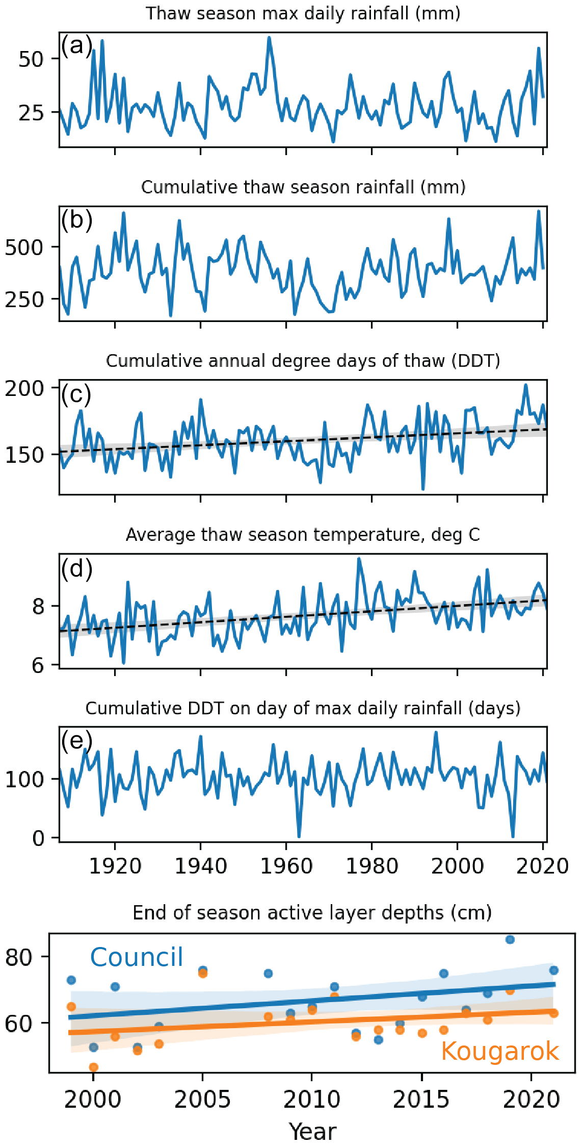
Figure 9 Nome Airport climate data (Alaska Climate Research Center Data Portal, 2022) and active layer thickness datasets. (a) The maximum daily rainfall, in millimeters, for the year's thaw period, defined by days in which degree days of thaw (DDT) are increasing versus the previous day. (b) The cumulative rainfall (in mm) that fell over the thaw period of that year. Both (a) and (b) appear cyclic over the past century. (c) Cumulative annual DDT for each year, which exhibits a statistically significant linear increase (95 % confidence interval). (d) Average temperature of the thaw days of a given year, which exhibits a statistically significant linear increase (95 % confidence interval) (e) The cumulative annual DDT on the day of the year of the single largest precipitation event. Despite potentially increasing cumulative DDT over the century, the timings of thaw initiation and large rainstorms appear to move in tandem, with a consistent ∼100 d between initial thaw and precipitation event. (f) Thickness of the active layer at two sites (Council and Kougarok) on the Seward Peninsula since 1999 from data derived from the CALM permafrost monitoring network (Brown et al., 2000; Nyland et al., 2021), whose upward trend is not statistically significant (95 % confidence interval).

Elsewhere in the Arctic, thaw slump activity has been linked to rising summer air temperatures (Lacelle et al., 2010; Lewkowicz and Way, 2019). In the Noatak Basin, northwestern Alaska, a high concentration of new thaw slumps occurred in the aftermath of an unusually warm and rainy May (Balser et al., 2014). These authors speculated concurrent thaw and rainfall may raise pore pressures in an active layer that would otherwise be drier and less thermally conductive; unsaturated active layers are more self-insulating than saturated active layers. However, the causes of small hillslope failures like those described in this study have not been extensively studied across the Arctic. Tracking hillslope disturbances at the scale of what we observed at Teller 47 (the visibly apparent scars of most individual failures are <10 m²) is only possible with high-resolution imagery such as that collected with a UAS and thus have limited temporal range for study. Future data compilations and modeling endeavors should determine the relative contribution of temperature versus precipitation to the frequency and magnitude of slope failures and gullying in the Arctic.

6 Conclusions

We quantified the timing and rate of surface movements in a discontinuous permafrost landscape using numerous approaches (UAS surveys, DGPS, and InSAR). Field-surveyed displacements of targets within and outside of lobes exhibited similar annual rates and do not appear sensitive to topographic factors like slope or drainage area. In contrast, mapped slope failures cluster at slope–area thresholds, but slope-stability models predicted many more failures could have occurred. This mismatch implies that permafrost hillslopes have unaccounted-for cohesion and/or throughflow pathways, perhaps modulated by vegetation, which stabilize slopes against high rainfall. Time series of InSAR displacements show accelerated movement in late summer, associated with intense rainfall and/or deep thaw, and cumulative annual displacements mirror cumulative annual rainfall. The changing role of water is therefore of equal importance as the changing thermal conditions in explaining ongoing topographic change in permafrost landscapes. Our results highlight the breadth and complexity of soil transport processes in Arctic landscapes and demonstrate the utility of using a range of synergistic data collection methods to observe multiple scales of landscape change.