the Creative Commons Attribution 4.0 License.
the Creative Commons Attribution 4.0 License.
 | 31 Jan 2023
Mineral surface area in deep weathering profiles reveals the interrelationship of iron oxidation and silicate weathering
Kyungsoo Yoo
Anthony K. Aufdenkampe
Edward A. Nater
Joshua M. Feinberg
Jonathan E. Nyquist
Mineral specific surface area (SSA) increases as primary minerals weather and restructure into secondary phyllosilicate, oxide, and oxyhydroxide minerals. SSA is a measurable property that captures cumulative effects of many physical and chemical weathering processes in a single measurement and has meaningful implications for many soil processes, including water-holding capacity and nutrient availability. Here we report our measurements of SSA and mineralogy of two 21 m deep SSA profiles at two landscape positions, in which the emergence of a very small mass percent (<0.1 %) of secondary oxide generated 36 %–81 % of the total SSA in both drill cores. The SSA transition occurred near 3 m at both locations and did not coincide with the boundary of soil to weathered rock. The 3 m boundary in each weathering profile coincides with the depth extent of secondary iron oxide minerals and secondary phyllosilicates. Although elemental depletions in both profiles extend to 7 and 10 m depth, the mineralogical changes did not result in SSA increase until 3 m depth. The emergence of secondary oxide minerals at 3 m suggests that this boundary may be the depth extent of oxidation weathering reactions. Our results suggest that oxidation weathering reactions may be the primary limitation in the coevolution of both secondary silicate and secondary oxide minerals. We value element depletion profiles to understand weathering, but our finding of nested weathering fronts driven by different chemical processes (e.g., oxidation to 3 m and acid dissolution to 10 m) warrants the recognition that element depletion profiles are not able to identify the full set of processes that occur in weathering profiles.
- Article
(8193 KB) - Full-text XML
-
Supplement
(595 KB) - BibTeX
- EndNote


1.1 Specific surface area in weathering
Weathering reactions cause dissolution and removal of elements from minerals. Some weathering reactions also produce secondary minerals that form in the place where the primary mineral has weathered, often along fractures or foliations in rock. Studies of rock weathering most often measure element and mineral content of weathering profiles to determine depletion (or enrichment) of elements and minerals. The removal of elements and the formation of secondary minerals as rocks weather increase the specific surface area (SSA, area of surface per unit mass of material) of the formation. Classic geochemical weathering models are based on elemental mass balance from measurements of major, minor, and trace elements in the bulk materials of a depth profile (Brimhall and Dietrich, 1987). Studies and models of chemical weathering suggest that morphologic boundaries should coincide with observable process-based transitions in weathering and pedogenesis (Rempe and Dietrich, 2014; Hasenmueller et al., 2015; Bazilevskaya et al., 2013; Brantley and Olsen, 2014; Brantley et al., 2013b; Maher, 2010; Riebe et al., 2017; Parsekian et al., 2015; Pedrazas et al., 2021; Gu et al., 2020; Brantley and Lebedeva, 2021).
Here we contribute to a series of co-located weathering studies that combine numerous geochemical and geophysical methods to identify the sequence of weathering processes over entire weathering profiles and below the water table at contrasting positions in a landscape. For this study, our goal was to understand how the generation of secondary minerals and SSA coincided with weathering processes and boundaries revealed by our previous studies of elemental depletion (Fisher et al., 2017) and soil biogeochemistry (Fisher et al., 2018) at the same forested hillslope sites over geochemically variable schist bedrock. We quantified primary and secondary minerals and measured the SSA over the same two 21 m deep drill cores for which we quantified major, minor, and trace elements (Fisher et al., 2017). These two 21 m deep cores were co-located with two of six soil pits along a ridgetop to toe slope to interfluve transect that were described and analyzed in detail (Fisher et al., 2018). Adding mineralogical and SSA measurements to this broader weathering study enabled us to explore formation processes for secondary minerals and the SSA that they produce.
Our aim was to drill at the ridgetop and the toe slope in a catena where Fisher et al. (2018) described the soil transect. Due to physical constraints of drilling equipment, we drilled at the ridgetop (Well 1) and on an interfluve (Well 2) that is 10 m below the ridgetop but not contained within the original soil hillslope transect. The soil morphology at the interfluve indicates that colluvium filled this position in the landscape, likely as periglacial mass movement during the Last Glacial Maximum (Carter and Ciolkosz, 1986; Merritts and Rahnis, 2022). After the colluvial influx the landscape experienced erosion that formed gullies in many parts of the forest, including our sampling location. Well 2 was drilled on a convex feature bounded by fluvial gullies, which we term interfluve to differentiate it from the top of the ridge while indicating its convexity (Schoeneberger et al., 2012).
We hypothesized that SSA would develop from the acid-driven weathering that is observable by elemental depletion trends and that morphological boundaries would coincide with changes in SSA. In these two drill cores we previously observed acid-driven elemental depletion weathering fronts at 7 and 10 m for the interfluve and ridgetop profiles, respectively (Fisher et al., 2017), and we therefore expected increasing secondary minerals and SSA at or near these depths. Rather, we observed a sharp SSA weathering front at 3 m deep and strongly increasing toward the surface due to the formation of secondary iron and aluminum oxides as well as oxyhydroxides. We did not observe SSA transitions near any of the many clearly visible soil morphological boundaries.
1.2 Terminology
The critical zone is defined to extend from the top of the vegetation canopy to the deepest limits of actively cycling groundwater (Brantley et al., 2007). This upper layer of the Earth has been termed the “critical zone” to facilitate interdisciplinary research questions and methods for interdependent hydrological, geochemical, geomorphic, biological, and other processes. A consequence of this interdisciplinary focus is that the many functional layers of the critical zone are often defined using different terms by different disciplines. We provide the following terminology for the weathering system in the present study.
We use bedrock to describe rock that has not been subject to alteration by physical or chemical weathering. We use the term weathered rock for rock that has been weathered but has not been physically mixed or mobilized, as evidenced by the retention of rock structure. Weathered rock includes isovolumetrically weathered rock and weathered rock with volumetric alteration that has not been mixed or mobilized. Weathered rock is commonly referred to as saprock, saprolite, and/or immobile regolith; saprock retains rock structure but is fractured and friable, with increased porosity that is susceptible to hydrolysis (Pope, 2015). Saprolite also retains rock structure but is friable and the secondary clay minerals give it plasticity when wet (Graham et al., 2010). Saprolite and saprock were not observed in the studied weathering profiles. The weathered rock we observed in this study retained rock structure that indicated no physical mixing, was strong and dense, and would break only along foliations. In the foliations chlorite and mica minerals would wipe off as a powder but had no plasticity when wet, even within the pedogenically altered soil horizons. We avoid the use of “regolith” because it has been used to describe in situ and mobilized weathered material, and in this discussion we prefer to differentiate between mobile and in situ rock (Pope, 2015). We consider weathered rock to include the soil C horizon, which is referenced by pedologists to describe the zone below which pedogenic alterations are no longer evident by field identification (NRCS, 1993).
We use the term soil to describe the physically mobile layer above weathered rock, in which physical and chemical weathering processes are most active and which develops genetic horizons from accumulation, translocation, and transformation of materials in the soil profile (NRCS, 1993). We consider soil to be synonymous with what geomorphologists recognize as the mobile regolith, which describes material that has been physically mixed or displaced and no longer retains rock structure (Pope, 2015).
1.3 Geological setting
The study site is the Spring Brook watershed (Fig. 1) located in southeastern Pennsylvania and within the Christina River Basin Critical Zone Observatory (CRB-CZO). The bedrock at the site is the Laurels Schist, a foliated, silvery, gray–green, quartz, plagioclase, muscovite, chlorite, garnet schist with minor biotite (mostly retrograded to chlorite) and accessory magnetite, epidote, tourmaline, apatite, and zircon (Blackmer, 2004). The Laurels Schist weathers along the planes in foliation and leaves platy segments of rock that remain virtually unweathered internally. The soils in Spring Brook are mapped as Manor Series soils (Official Soil Series Descriptions. Natural Resources Conservation Service, United States Department of Agriculture, 2012). These Typic Dystrudepts are highly micaceous with weak structures and coarse sandy clay loam textures. The abundant coarse fragments in all of the soils in Spring Brook are composed of angular platy rock fragments of schist called channers. Fisher et al. (2018) calculated a minimum landscape age of 19 kyr for Spring Brook summit and an erosion rate of 50 m Myr−1.
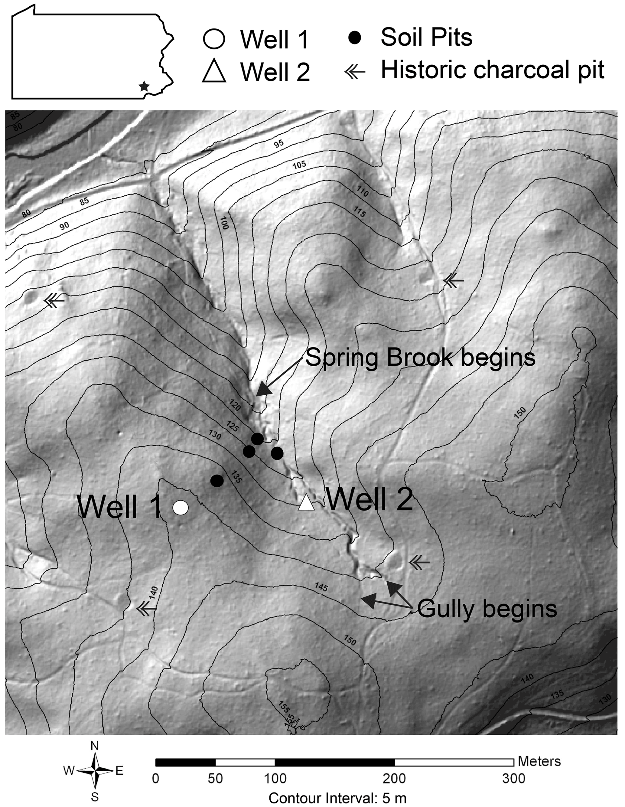
Figure 1A ground-return lidar hillshade image provides a site map of the Spring Brook watershed in the Laurels Preserve in southeastern Pennsylvania. In addition to Well 1 and Well 2, we sampled a transect of soil pits to characterize the influence of landscape position on SSA and other biogeochemical properties (Fisher et al., 2018). The contour interval is 5 m, and features discussed in the text, such as historic charcoal pits and gullies, are labeled (lidar DOI: https://doi.org/10.5069/G9T43R00).
Spring Brook is a first-order watershed that covers 9.6 ha, with a 250 m long spring-fed perennial stream. Summit and back-slope soils in Spring Brook are forming on bedrock. In the lower concave portions of the watershed, colluvium filled the valley through periglacial mass movement during the Last Glacial Maximum. In the 1800s this land was logged, which resulted in erosion. We see evidence of this logging practice, in which the logs were turned to charcoal on site, because the depositional positions throughout the landscape contain soil profile lenses with charcoal. Up-gradient from the stream is a 150 m long, 1 m deep, historic gully that eroded during the logging era and is no longer actively eroding. The gully has been stable long enough to develop an A horizon with significant organic matter accumulation throughout the extent of the swale.
The Spring Brook watershed is a second growth mixed chestnut, oak, and hickory forest of approximately 120–150 years in age and was logged for one to two cutting and planting cycles of 25–30-year-old hardwood trees to provide charcoal for local smelting operations beginning around 1825 (Lesley, 1859; Shields and Benson, 2011). We interpret the level, 2–3 m diameter circles in the lidar imagery as remnants of charcoal production, and each of these circular features contains charcoal and is near a former road (Fig. 1). The property was purchased for hobby farming in the early 1900s, which did not involve tillage, and was used for cattle grazing beginning in 1946. In 1967 the Brandywine Conservancy dedicated the property as the Laurels Preserve and ended grazing activity (Shields and Benson, 2011).
The present climate in Spring Brook is humid continental with mean annual precipitation (MAP) of 1246 mm and a mean annual temperature (MAT) of 10.85 ∘C. The full annual temperature range was −6 to 29 ∘C (1961–1990, Coatesville, PA, https://www.usclimatedata.com, last access: 1 September 2016). Paleoclimate records based on pollen type between 18 and 12 ka estimate annual lows of −12 ∘C and highs of 16 ∘C, which represents a periglacial climate at the Last Glacial Maximum. By 9 ka the temperatures were −4 to 22 ∘C, with a gradual shift to present-day temperature ranges (Prentice et al., 1991).
2.1 Rotosonic drilling
To capture the subsurface topography of weathered materials in Spring Brook, we selected the ridgetop (Well 1, 143.886 m a.s.l.; 39.9195025∘, −075.7891562∘; https://app.geosamples.org/sample/igsn/IESW10006) and interfluve (Well 2, 134.164 m a.s.l.; 39.9194885∘, −075.7879179∘; https://app.geosamples.org/sample/igsn/IESW10007) for drilling. Two 21 m deep boreholes were drilled into the Laurels Schist formation in August 2012. Drilling of additional boreholes was precluded by logistical and financial challenges in the remote, densely forested, steep terrain. Samples were acquired using a Geoprobe Rotosonic (model 8140LC) mid-sized track-mounted drilling rig. The drilling method employed was the “4×6” method, which involves two hollow bits that yield a 4 in. (10.16 cm) sample diameter and a 6 in. (15.24 cm) borehole diameter. Sample intervals up to 10 m in Well 1 and 5 m in Well 2 were drilled with air (i.e., no fluids) to maximize recovery and nearly eliminate contamination. Deeper intervals alternated between no drilling fluid and EZ-MUD® polymer emulsion (by Baroid IDP) to enable drilling to proceed in a timely manner. The drill segments were 1.52 m and were inserted into a plastic sleeve immediately after recovery. While the cores were partially pulverized by the Rotosonic drilling action and segmented due to the foliated nature of the schist, the recovered volumes were 68 %–100 % for core segments drilled without fluid. Where EZ-MUD fluid was used, the recoveries ranged from 17 %–83 % and contained large rock pieces with no pulverized material. Missing sample intervals in the dataset occur where segments were drilled with fluid. Drilling progress was hindered in Well 2 when the drill bit broke after approximately 12 m of recovery. In the laboratory the cores were removed from their plastic sleeves, photographed (Supplement), and divided into intervals of approximately 10 cm. Samples were oven-dried at 60 ∘C, sieved to 2 mm, and weighed. The drilled wells were maintained with flexible liners (FLUTe™ blank liners) that can be removed for measurements and future installations.
2.2 Soil sampling
In addition to drilling, soil pits were hand-excavated to ∼1 m deep within a few meters of the boreholes (Pit 1, ridge: 143.932 m a.s.l., 39.9194572∘, −075.7892333∘, https://app.geosamples.org/sample/igsn/IESW10001; Pit 2, shoulder: 139.949 m a.s.l., 39.919783∘, −75.7888499∘, https://app.geosamples.org/sample/igsn/IESW10002; Pit 3, planar back slope: 129.989 m a.s.l., 39.919926∘, −75.7885518∘, https://app.geosamples.org/sample/igsn/IESW10003; Pit 6, toe slope: 123.096 m a.s.l., 39.9200122∘, −75.7883606∘, https://app.geosamples.org/sample/igsn/IESW10005; Pit 4, swale: 39.919863∘, −75.788162∘, https://app.geosamples.org/sample/igsn/IESW1001C; Pit 5, interfluve: 133.108 m a.s.l. 39.9195557∘, −075.7878866∘, https://app.geosamples.org/sample/igsn/IESW10004). After detailed soil description (Official Soil Series Descriptions. Natural Resources Conservation Service, United States Department of Agriculture, 2012), soil sample collection was guided by morphological horizons. Soil materials were sampled across the entire width of the upslope side of the soil pit to integrate heterogeneities. Soil samples were homogenized in the lab, oven-dried, sieved to 2 mm, and weighed. We did not collect forest litter.
2.3 Specific surface area (SSA)
Samples from the fine fraction (<2 mm), which was mostly generated during grinding associated with drilling, were retained for measurement of SSA. Oven-dried (60 ∘C) samples were degassed at 150 ∘C for a minimum of 4 h in N2 saturation (Mayer and Xing, 2001), weighed, and analyzed using N2 adsorption on a Micromeritics TriStar II 3020. Specific surface area (mineral surface area per unit mass of soil) was calculated with an 11-point isotherm using the BET multipoint isotherm method (Brunauer et al., 1938). For each sample, we measured SSA on three sample treatments to collect information about organomineral associations and extractable oxides. First, untreated samples that may contain organic matter were measured (Dataset S1), then the samples were oxidized at 350 ∘C for 12 h to remove organic matter (Keil et al., 1997), which is the most widely used method to prepare mineral surfaces for N2 adsorption (total SSA). It is well-understood that some mineral transformations can occur under these conditions, but tests by multiple researchers show that these treatments minimally alter total SSA (Keil et al., 1997). For example, our tests of the effects of heating on three soil types and synthesized iron minerals revealed that SSA increased with increased heating temperatures from 150 to 350 ∘C (unpublished lab results). Regardless, all samples for our study were subjected to the same pretreatments, so internal comparison is not a concern. Finally, Fe and Al oxides were removed by the citrate–dithionate method (Burt, 2004) to measure the SSA of primary and secondary silicate minerals (SSASi) and calculate the contribution of extractable oxides to SSA as the fraction of Fed SSA, where Fed . Although the citrate–dithionate extraction was performed on all SSA samples, the elemental composition of extracts was only determined for some intervals from Well 1. In sample intervals where replicate measurements occurred, the mean is reported.
SSA of naturally weathered minerals (e.g., sheet silicates or needle-like oxides) substantially exceeds that of mechanically ground minerals (White et al., 1996; Brantley and Mellott, 2000; Knauss and Thomas, 1989). To confirm that partial pulverization from Rotosonic drilling did not interfere with our estimate of naturally derived SSA, we analyzed SSA on samples that were pulverized in a tungsten carbide ring mill to a particle size that is finer than that produced by Rotosonic drilling. Rocks from Ridge Well 1 at 13 and 16 m were pulverized to D50<20 µm (by laser particle size analysis) and yielded SSA of 6.27 and 6.37 m2 g−1, respectively. If the same particles were perfect cubes rather than mineral-shaped, those samples would yield SSA of only 0.15 m2 g−1 (calculated with density 2600 kg m−3). Rotosonic samples from the finest samples from Ridge Well 1 at 13 and 16 m were sand-sized and ranged in SSA from 3–5 m2 g−1. These results validate the fact that natural mineral structure dominates the SSA measured on drill-pulverized samples.
2.4 Inventory of total mineral surface area
We determine the cumulative inventory of total mineral surface area per given ground surface area (surface area inventory, SAI, in unit dimensions of L2 L−2) from the land surface to the lower depth (z) limit of H as
where SSA is the total mineral specific surface area (L2 M−1) in the depth z, ρ is the bulk density of weathered material (ML−3), and f is the coarse fraction (>2 mm, MM−1). Because the depth to unweathered bedrock varies, we designed SAI to be calculated to a depth of choice (i.e., z=H with units of L).
We calculate SAI beginning at the ground surface and increasing within lower depth limit because the surface is a natural boundary and because we cannot assume the terminal depth of significant weathering and SSA generation. Furthermore, calculating and visualizing inventory in this direction follows conventions used for soil organic carbon and cosmogenic radionuclide inventories (Jobbágy and Jackson, 2000). The noteworthy points in the visualization are the slope and the changes in slope, which enable us to identify process-driven transitions.
2.5 Bulk density
Bulk density measurements for Well 1 were taken directly from the ground surface to the depth of 3.41 m from a nearly continuous set of 2.4 cm diameter cores that were collected using a soil recovery probe (AMS 424.03 custom-built to 0.91 m) from an excavated soil pit a few meters from the well. Bulk density for Well 2 was measured using the same method for the first 1.80 m. Soil cores were segmented in the lab at intervals no greater than 10 cm, air-dried, oven-dried for 48 h at 60 ∘C, and weighed. The USDA standard drying temperature is 110 ∘C (Burt and Staff, 2014), but we chose 60 ∘C to minimize the degradation caused by heat on phyllosilicates and metastable oxide minerals. The stability of these minerals was a concern for X-ray diffraction (XRD) analysis and other biogeochemical measurements in the soil profile. Subsamples for SSA received additional treatment, as described in Sect. 3.3.
We were not able to directly measure bulk density from depths of 5 to 21 m at Well 1 and from 4 to 21 m at Well 2 due to the partially pulverized drill cores recovered from the Rotosonic method. For these intervals we estimated bulk density based on average rock fraction and density of rock chips. The specific gravity of rock chips was measured by water displacement: dry rock chips were weighed in air and the volume of the rock was determined by the mass of water displaced by the rock chips, with two to five replicates for each interval. Because rock chips had low permeability, we did not coat them with plastic or wax, as is necessary for submerging soil or friable material (Burt and Staff, 2014). Rock chip density values in each well did not vary systematically with depth. Average rock chip density for Well 1 (n=63) was 2700 ± 100 kg m−3, and for Well 2 (n=108) the average was 2770 ± 110 kg m−3. Where we have rock chip density measurements and bulk density cores in the top 3.41 m, the bulk density was 53 %–69 % lower than rock chip density. We know that the influence of weathering decreases with increasing depth, but we do not observe an increase in rock chip density with depth, so we set the bulk density estimate as a constant. Thus, for deep bulk density estimates we used 68 % of the rock chip density for each interval to capture the high end of the bulk density range observed from 0–3 m, which yields conservative underestimates in inventory calculations. The bulk density values below 5 m averaged 1830 ± 70 kg m−3 (n=25) in Well 1 and 1880 ± 90 kg m−3 (n=16) in Well 2.
2.6 Characterization of bulk mineralogy
To examine the links between mineral surface area and mineralogy, we characterized the mineralogy of bulk samples using X-ray diffraction (XRD) on a Siemens D-500 diffractometer with a 2.2 kW sealed cobalt source at the University of Minnesota Characterization Facility. Samples were pulverized on a tungsten carbide ring mill to 6 µm (D90) and combined with a 10 % zincite internal standard (Eberl, 2003). The mixture was combined using an agate mortar and pestle wetted with ethanol and was packed into a holder and scanned from 5 (machine minimum) to 75∘ 2θ using Co Kα radiation with 0.02∘ steps and a dwell time of 2 s per step on a continuously rotating sample stage.
XRD spectra were converted to Cu Kα wavelengths for easy comparison with earlier studies using JADE 7.0 software (Materials Data, Inc.) and exported as ASCII text for analysis. Peak intensities were manually normalized in spreadsheet form, setting the zincite 2.476 Å peak as 10 %. Major minerals were identified and quantified using non-interfering peaks and normalized by expected peak intensities: quartz 1.8179 Å (0.14 intensity), plagioclase group 3.17–3.21 Å (1), muscovite 9.95 Å (0.95), and clinochlore (chlorite group) 4.77 Å (0.7).
2.7 Clay mineralogy
Given the expected disproportionate contributions of clay-sized minerals to mineral SSA, we separately characterized their mineralogical compositions. The clay size fraction was isolated by gravity sedimentation using a suction apparatus (Jackson and Barak, 2005). Isolated clay-sized fractions were pretreated in multiple steps to remove carbonates (sodium acetate–acetic acid solution), organic matter (bleach method), and extractable iron oxides (citrate–dithionite) (Burt, 2004; Jackson and Barak, 2005). Because our samples were low in carbonate content and not extremely high in organic matter, we were not concerned that cementation would hinder clay isolation prior to pretreatment. We expect that if some clays were lost during fractionation, the ratios of different clays are likely to be maintained within the detection sensitivity of XRD.
Clays were divided and saturated with potassium or magnesium and were mounted by oriented suspension on glass coverslips. Saturated samples were scanned from 5 to 18∘ (K-saturated) and 5 to 36∘ (Mg-saturated) 2θ using Co Kα radiation. Potassium-saturated samples were heated to 500 ∘C for 1 h and scanned again from 5 to 18∘ 2θ. Magnesium-saturated samples were further saturated with ethylene glycol and scanned from 5 to 18∘ 2θ. Clay XRD methods may have been impacted by pulverization by sonic drilling action, which broke primary minerals into pieces that are small enough to partition with clays in our gravity settling separation, and the pulverized particles may inhibit the secondary phyllosilicates from orienting parallel to the glass slides.
We have chosen not to quantify clay minerals in this study for the following reasons. Repeated chemical rinses and vacuum separation of clay particles from the bulk sample may bias quantification of secondary phyllosilicate minerals. Additional bias may be introduced into the quantification of samples from greater depths collected from Rotosonic drill cores because pulverization by sonic drilling action broke primary minerals into pieces small enough to separate from clays, inhibiting the secondary phyllosilicates from orienting parallel to the glass slides.
2.8 Iron mineralogy
We used rock magnetic measurements to characterize the iron-based magnetic mineral assemblage by mineral species, quantity, and size (Dunlop and Ozdemir, 2007) on a subset of specimens from Ridge Well 1. Samples were pressed into 6 mm diameter pellets under pressure in a mixture of rock powder with SpectroBlend powder (81.0 % C, 2.9 % O, 13.5 % H, 2.6 % N). Room-temperature and low-temperature saturation isothermal remanence (RTSIRM, LTSIRM) was measured on five of the specimens using a Magnetic Properties Measurement System (MPMS, Quantum Designs). A room-temperature vibrating sample magnetometer (VSM, Princeton Measurements) was used to obtain hysteresis loops for all samples. We applied a 1.25 T maximum magnetic field and measured bulk hysteresis parameters, saturation magnetization (Ms), saturation remanence (Mr), coercivity (Bc), and coercivity of remanence (Bcr). To isolate the magnetization of hematite and goethite, we sequentially removed the magnetization associated with magnetite using a 200 mT alternating field demagnetization step and then removed the magnetization associated with goethite using a 100 ∘C thermal demagnetization step.
2.9 Extraction chemistry
We used the citrate–bicarbonate–dithionite (CBD) method to remove free and amorphous iron oxide secondary minerals from samples (Holmgren, 1967; Burt, 2004; Jackson and Barak, 2005). In each instance we applied this method to samples from which organic matter was previously removed. In the CBD solution, iron is reduced with sodium dithionite. Sodium citrate chelates the reduced iron to keep it in solution. Sodium bicarbonate buffers the solution to pH 7.3, and the method was performed at room temperature. The extracted fluid from a subset of 17 samples from Ridge Well 1 was analyzed using inductively coupled plasma–optical emission spectroscopy (ICP-OES) (at Research Analytical Lab, University of Minnesota) to measure the concentration of 27 elements.
CBD extraction was developed to remove Fe oxides, especially amorphous forms, but the method is also shown to remove hydroxy-interlayered aluminum as well as some Al oxides (Shang and Zelazny, 2008). Iron minerals removed by CBD extraction include goethite, hematite, and maghemite, and submicron-sized magnetite may also be extracted (Hunt et al., 1995). While acknowledging the variety of minerals extracted by the CBD method, we refer to these as “extractable oxides” for brevity.
2.10 Seismic multichannel analysis of surface waves (MASW) survey
A geophysical seismic survey using multichannel analysis of surface waves (MASW) was performed along a transect that ran directly from Well 1 to Well 2. The MASW survey used a 16 lb sledgehammer as the seismic source in conjunction with a 24-channel Geometrics Geode seismograph and 4.5 Hz geophones. The geophones were spaced 1.5 m apart (34.5 m spread) with a source offset of 10.5 m from the end the geophone spread to avoid near-field effects in surface wave generation. At each shot location we stacked five hammer blows to boost the signal-to-noise ratio. The entire line was then shifted 3 m (twice the geophone spacing) and the process repeated for a total survey line length of 141 m. The seismic data were analyzed using SeisImager/SW. This approach resulted in estimates of seismic shear wave velocity down to ∼20 m depth along the transect.
3.1 Morphology
The Manor Series soils are coarse–loamy, micaceous, mesic Typic Dystrudepts that exhibit morphological differences associated with landscape position. Detailed morphology of six soil pits at contrasting landscape positions within the Spring Brook catchment is described by Fisher et al. (2018). While hand-excavating soils, we identified the C horizon at 0.84 m near Well 1 by observation of rock structure, silvery gray–green color, undisturbed foliation orientation, and the absence of pedogenic features at this depth within the hand-excavated soil pit. Near Well 2 we excavated a soil pit to 1.24 m, where we observed yellowish brown coloration, pedogenic mottling, and some disruption of rock fragments, so we considered this a B horizon. A grid of soil recovery probes into the bottom of the soil pit indicated a consistent depth where the color changed to the silvery gray–green bedrock color at approximately 1.50 m, which we assigned as the C horizon. In summary, the depth of the boundary of soil to weathered rock occurs at 0.84 m at Well 1 and 1.50 m at Well 2.
3.2 Mineral specific surface area and extractable iron and aluminum oxides
Total mineral specific surface area (SSA, Fig. 2) showed strong depth trends in the upper 3 m at both wells. The total SSA abruptly increased above 3 m, from 2–5 m2 g−1 below to values of ∼12 m2 g−1 at 1.5 m and up to 22 m2 g−1 near the surface. No depth trends were discernable from 4 to 21 m depth. Well 2 had higher a surface area inventory (SAI) in the upper 3 m due to greater accumulations of fine (<2 mm) material within its depositional morphology (Fig. 2).
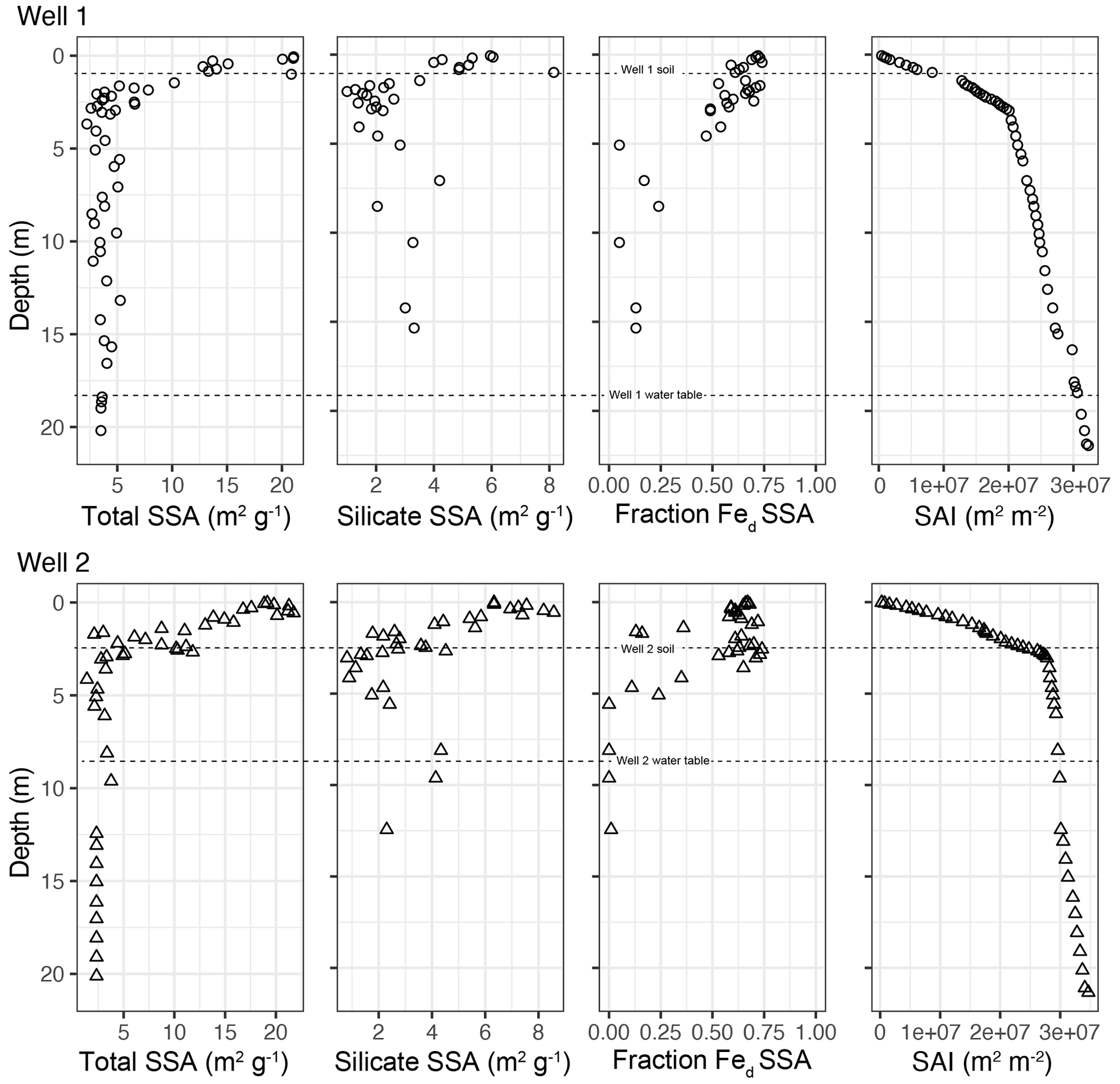
Figure 2Total SSA vs. depth, silicate SSA, fraction of SSA contributed by citrate–dithionite extractable iron (Fed), and surface area inventory (SAI) reveal that SSA increases toward the ground surface and exhibits an abrupt increase near 3 m. Fed SSA reveals that most intervals above 4 m contribute over 50 % of SSA, and below 4 m, <25 % of the SSA is contributed by extractable iron and aluminum minerals. The mean water table for Well 1 was 19 m, and for Well 2 the mean was 7 m. We monitored the water levels using a Decagon CTD10 from December 2013 through January 2015; Well 1 water levels ranged from 17.70–20.27 m, and Well 2 water levels ranged from 6.85–8.33 m.
Silicate SSA (SSASi) measured on samples after citrate–bicarbonate–dithionite extraction mirrored trends in total SSA. SSASi, the combined SSA of primary minerals and secondary phyllosilicates, was responsible for up to 10 m2 g−1 of SSA at the ridge and 9 m2 g−1 at the interfluve (Fig. 2).
The SSA contributed by extractable oxides (Fed SSA), calculated by difference (i.e., ), followed similar increases as total SSA and SSASi over the top 3 m of the drill cores. Fed SSA contributed 36 %–81 % of the SSA found in samples within the top 3 m in both drill cores and reached 15 m2 g−1 at the ridge and 14 m2 g−1 at the interfluve (Fig. 2). Immediately below the 3 m boundary the Fed contribution to SSA was very low. The fraction of SSA contributed by extractable oxides at Ridge Well 1 is 48 %–81 % from 0–3 m deep and 5 %–25 % below 3 m. At Interfluve Well 2 extractable oxides contribute 36 %–77 % of SSA from 0–1.5 m, 13 %–74 % from 1.5–3 m, and 10 %–15 % below 3 m.
The concentration of total Fe (as Fe2O3) hovers close to 10 % along the top 4 m, while the total Al (Al2O3) decreases by about 5 % but hovers around 20 % (Fig. 3). Despite less total Fe vs. Al in the bedrock system, the extractable iron was twice as abundant. The contribution of extractable oxides to total SSA ranged 36 %–81 % of the total SSA over the top 3 m at both landscape positions. Especially significant to this finding is that the extraction removed only <0.1 % of the total sample mass at each interval, meaning that the vast majority of the SSA came from an extremely small mass of sample. The depth profile of total iron shows very little depletion, and total aluminum shows a gradual depletion over the top 4 m where the extractable forms of these elements contributed abundant SSA (Fed SSA in Fig. 3).
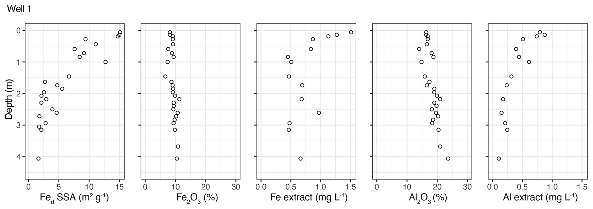
Figure 3Fraction of SSA contributed by citrate–dithionite extractable iron (Fed SSA) for the upper 4 m profile compared to the percent of bulk as Fe or Al as well as to the concentration of Fe or Al in the citrate–dithionite extract.
Fed SSA increased in direct proportion to SSASi over the top 3 m in both drill cores (Fig. 4). None of the changes in total SSA, Fed SSA, and SSASi coincide with the transitions from soil to weathered rock (0.84 and ∼1.50 m for ridge and interfluve, respectively), nor do they correlate with water table fluctuations (Fig. 2).

Figure 4Correlation of Fed SSA with silicate SSA for data from 0–3 m reveals a strong positive correlation between iron and silicate SSA. The correlation holds true at Ridge Well 1 and Interfluve Well 2.
The plot of cumulative inventory of total mineral surface area (SAI, Figs. 2 and 4) reveals where changes occur in mineral surface area production. We applied a segmented linear regression model (Muggeo, 2008) to identify intervals with similar slopes and the break points between these intervals. We iteratively applied segmented regression to optimize fit and break points for each SAI profile using SAI as the dependent variable in the regression analysis and depth as the independent variable (Fig. 5). Our iterations tested the number of break points that yielded the highest R2. Ridge Well 1 had two break points at 1.50 ± 0.08 and 3.11 ± 0.07 m (, , m2 m−3, R2=0.9981). Interfluve Well 2 had three break points at 1.02 ± 0.03, 2.22 ± 0.06, and 2.82 ± 0.02 m (, , , m2 m−3, R2=0.9994). The largest relative change in slope within each profile occurred near 3 m at both drill cores.

Figure 5The surface area inventory (SAI) reveals trends in the accumulation of mineral surface area. The inset image (b) shows the full depth trend, while the larger image (a) reveals the top 5 m. The segmented linear regressions reveal slope changes that do not coincide with morphologically identified boundaries. Gray points in the inset are calculated from interpolated (linear) SSA.
These break points do not correlate well with morphologic features observed from soil pits or drill cores, such as the water table (∼19 and ∼7 m for Wells 1 and 2, respectively) or the boundary of soil to weathered rock (0.84 and 1.50 m for Wells 1 and 2, respectively) (Fig. 2). Nor do the break points correlate with the depths of elemental Ca depletion at 10 m in Well 1 and 7 m in Well 2 (Fig. 6).
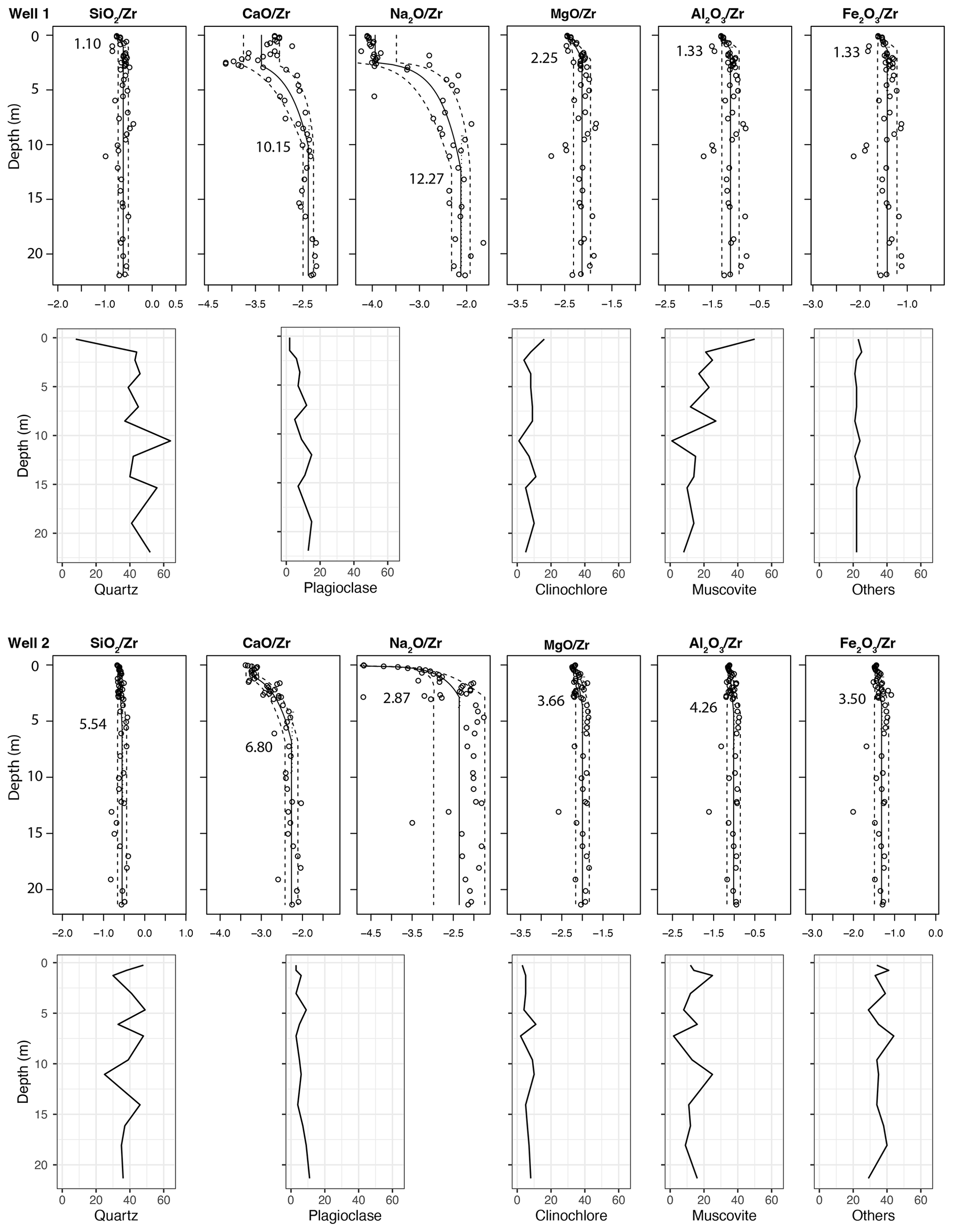
Figure 6Percent distribution of the four major mineral group samples is shown alongside elemental mass balance for dominant elements in each mineral group for each well. Modeled depths of elemental depletion are labeled on each element profile (confidence intervals are tabulated in SI). Mineralogy is variable with depth in both wells, lacking distinctive weathering trends. Other minerals include may include magnetite, hematite, goethite, epidote, garnet, zircon, and others that are in quantities too low for XRD detection or in crystal forms that are amorphous to XRD.
3.3 Mineralogy
Quantitative analysis of bulk XRD revealed that the Laurels Schist is mineralogically variable (Fig. 6), with few discernable depth trends. The bulk primary mineral matrix is composed of quartz, plagioclase, muscovite, and chlorite group minerals (Fig. 7). Of these, primary plagioclase group minerals show the only consistent trend, with relative abundance decreasing toward the surface (Fig. 6). In Ridge Well 1 plagioclase decreases from 15 % at 7 m to 2 % in the near-surface. In Interfluve Well 2 we observe 11 % plagioclase at the base of the profile, which decreases to 3 % in the near-surface XRD data. These results are reinforced by the element mass balance profiles of Ca and Na, which show depletion in the upper 7 to 10 m, because Ca and Na primarily occur within plagioclase group minerals within the Laurels Schist bedrock.
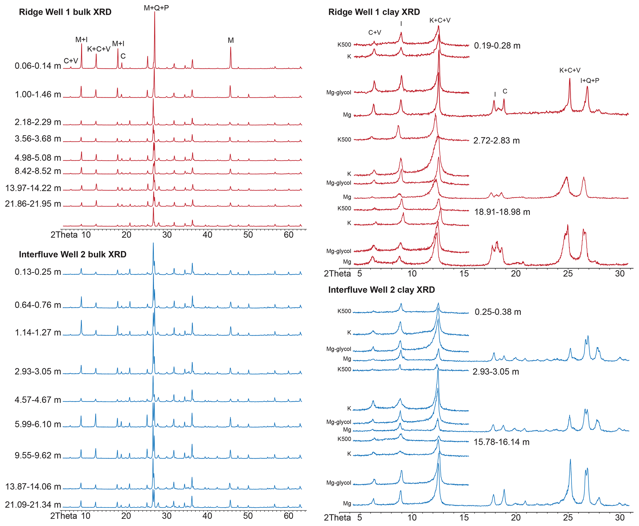
Figure 7Representative XRD spectra for both wells. Bulk XRD was analyzed on random mounts of pulverized sample with a zincite internal standard (peaks in : 2.47635.65(1), 2.81631.35(0.71), 2.60233.93(0.56)). Clay XRD is performed on oriented suspension mounts of pretreated sample (see Sect. 2.7). Mineral groups are generalized and abbreviated as C: chlorite, I: illite, K: kaolinite, M: mica, P: plagioclase, Q: quartz, V: vermiculite.
Although muscovite and chlorite group (i.e., clinochlore) minerals generally oscillate with depth in both wells, peaks for illite–mica and chlorite–vermiculite increase above 2 m within Ridge Well 1, but not for Interfluve Well 2 (Figs. 6 and 7). Elemental depletion of Mg, which primarily occurs in chlorite group minerals, occurs above 2.25 m in Well 1 and above 3.66 m in Well 2. The elemental depletion of Al follows a similar trend as Mg and Fe, with depletion above 1.33 m in Well 1 and above 4.26 m in Well 2.
Clay XRD spectra (Fig. 7) provide evidence that chlorite (14 and 7 Å), illite (10 Å), and vermiculite (14 Å decreasing to 10 Å on heating) occur throughout both profiles and that very little kaolinite is present (i.e., the 7 Å peak is not greatly reduced upon heating to 500 ∘C, suggesting it is a second-order chlorite peak) (Moore and Reynolds, 1997; Jackson and Barak, 2005; Poppe et al., 2001). In Ridge Well 1 the peaks for illite and vermiculite increase in intensity in the upper 3 m (Fig. 7). Trends in Interfluve Well 2 are not as clear because the XRD spectra are variable in Well 2, but illite and vermiculite have higher intensity in the 1.27 and 0.76 m spectra than the deeper intervals.
3.4 Magnetic mineralogy
Analysis of induced and remanent magnetizations for a small subset of Spring Brook samples from the ridge reveals a small quantity of primary magnetite within all Laurels Schist samples. Soils inherited minute quantities of this magnetite from the parent rock but also display fine-grained magnetite (<300 nm), likely pedogenic, enriched in near-surface samples. Of the bulk soil, up to 16 % goethite was detected in near-surface samples, while the same intervals contain <0.5 % magnetite and a similarly small quantity of hematite. Ilmenite was also identified in samples of both the Laurels Schist and its overlying soil. Of the extracted phases, 40 %–75 % were iron minerals, primarily goethite, but some intervals include minor contributions from fine-grained magnetite (<300 nm), hematite, and ilmenite. Most of the Fe-based mineral assemblage in the soil appears to be poorly crystalline goethite, which is consistent with field observations of yellowish colors within the soil (Fig. 9).
3.5 Seismic multichannel analysis of surface waves (MASW)
The seismic multichannel analysis of surface waves (MASW) survey revealed a gradual increase in seismic shear wave velocity with increasing depth for both wells (Fig. 8). Near Ridge Well 1, seismic shear wave velocity was 160 m s−1 at the surface, increasing to 300 m s−1 at 6–7 m and to 500 m s−1 at 14 m. Near Interfluve Well 2, velocities were 300 m s−1 at the surface and increased to 500 m s−1 at 10 m. The depth to 500 m s−1 velocities became increasingly shallow along the transect from Well 1 to Well 2. Shear wave velocities of 500 m s−1 are interpreted as soft rock and are not increased by water saturation (Lowrie, 1997). The soft rock velocities seem to conflict with rock chip densities, which average around 2700 kg m−3 in both wells. Foliation in the Laurels Schist results in discontinuous rock, which effectively slows seismic wave propagation, resulting in low velocities despite the high density rock chips (Clarke and Burbank, 2011, 2010; Eppinger et al., 2021). MASW surveys do not reveal any sharp transitions at ∼3 m depth or any of the other depths where we observed changes in mineral SSA. Near the surface by Well 2 we see material of intermediate velocity, which we interpret as the colluvial deposit.

Figure 8MASW cross section from Well 1 on the left to Well 2 on the right, revealing an increase in rock properties from the ground surface, with no subsurface structures detected. Near the surface by Well 2 we see material of intermediate velocity, which we interpret as the colluvial deposit. The S-wave velocities reach a maximum at 500 m s−1 to a depth of 14 m deep at Well 1, which tapers to 10 m deep at Well 2.
4.1 Secondary mineral and SSA formation separated from elemental depletion
We found a sharp increase in specific surface area and extractable secondary iron and aluminum oxide minerals starting at 3 m depth and increasing strongly toward the surface at both landscape positions (Figs. 2, 4, and 8). The extractable secondary iron and aluminum oxide minerals were responsible for 50 % to 75 % of SSA above 3 m (Figs. 2, 3, 8, and 9). Non-extractable silicate minerals accounted for the balance of the increased SSA above 3 m, or 25 % to 50 % of total SSA at these depths. These non-extractable secondary silicate minerals were likely various forms of vermiculite and illite, the bulk and clay fraction XRD of which have been observed in increased abundances in the upper 2–3 m (Fig. 7) and which form in many intermediate forms during the weathering of muscovite and chlorite group primary minerals (Fig. 10).
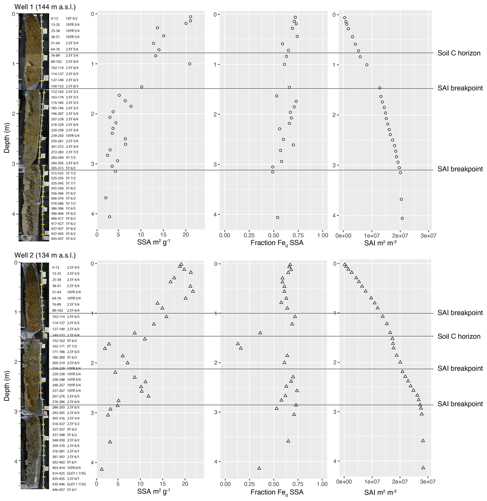
Figure 9Images of recovered drill core to ∼4.5 m with dry Munsell color aligned with data on total SSA vs. depth, fraction of SSA contributed by citrate–dithionite extractable iron (Fed), and surface area inventory (SAI). Images of drill cores indicate color change at the soil C horizon boundary, which is clear in Well 1 but obscured by the core recovery interval in Well 2. Images reveal yellow–orange hues of iron oxide presence in the cores to at least 3 m in Well 1 and to ∼3.25 m in Well 2. Data reveal that SSA increases toward the ground surface. The Fed SSA fraction reveals that most intervals above 4 m contribute over 50 % of SSA.
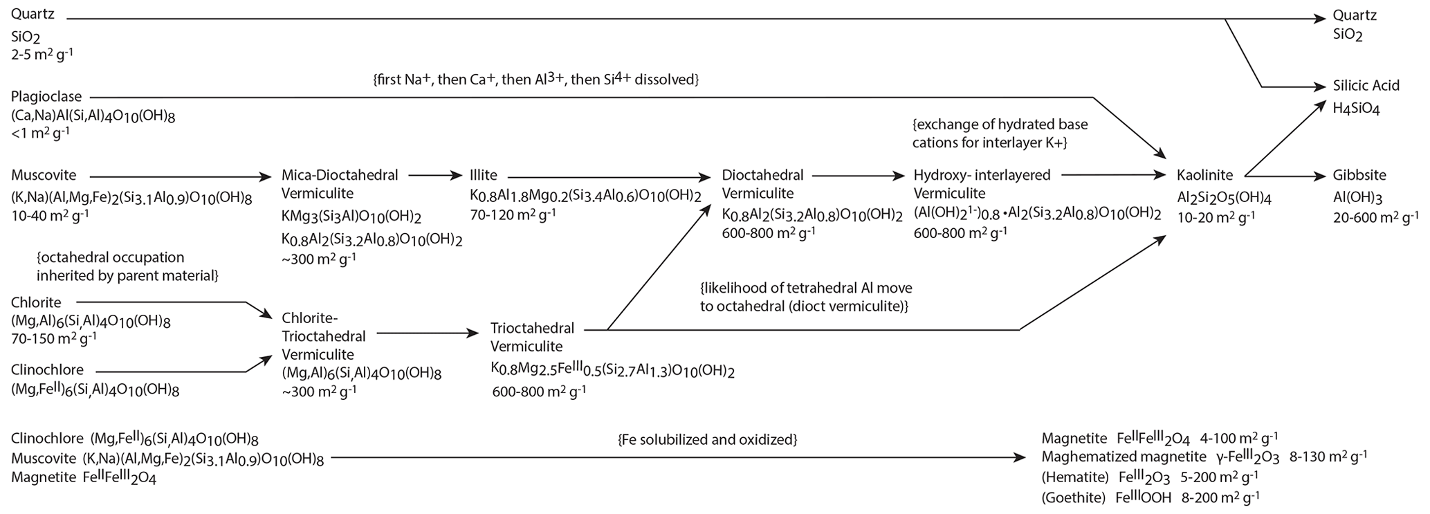
Figure 10Weathering pathways for the Laurels Schist, with major primary minerals listed on the left of the diagram flowing to their observed secondary products. The primary minerals include quartz, plagioclase, muscovite, chlorite–chlinochlore, and magnetite. The secondary minerals include illite, vermiculite, kaolinite, gibbsite (interpreted to be extracted Al), maghemite, hematite, and goethite. We include generalized chemical formulas and SSA range for each mineral. Minerals were identified by XRD and magnetic mineralogy.
We had hypothesized that secondary minerals and SSA would develop from the acid-driven weathering that is observable by elemental depletion trends for base cations Ca, Na, and Mg. Our findings clearly show, however, that depths of elemental depletion fronts vary widely by element and by location and are physically separated from secondary mineral and SSA formation fronts. Elemental depletion of base cations initiated at different depths for each element and location. Ca depletion began at 10.1 and 6.8 m for Wells 1 and 2, respectively; Na depletion started at 12.3 and 2.8 m, and Mg depletion initiated at 2.3 and 3.7 m (Fig. 6).
An alternate hypothesis was that secondary minerals and SSA might form near morphological boundaries, such as a visible soil horizon boundary or at the top of the water table. Our findings show that such morphological boundaries, however, are far from the secondary mineral and SSA formation front. The transition from B to C soil horizons occurred at 0.84 and 1.5 m at Wells 1 and 2, respectively (Fig. 2). The mean water table depth was 19 and 7.5 m (Fig. 2).
All measures of secondary mineral formation have sharp fronts occurring over a narrow depth range of 2.82 to 3.11 m at both locations. This depth did not coincide with any of the elemental depletion fronts or morphological boundaries. Furthermore, we did not observe any of the more subtle SSA transitions near any of the many clearly visible soil morphological boundaries (Fig. 5). We are forced to conclude, therefore, that another process must be driving the formation of secondary minerals and SSA.
Other studies find that the depth distribution of extractable oxides depends on soil type and morphology. Aburto and Southard (2017) studied glacial deposits in the Tahoe region in which the quantity of extractable oxides increased with decreasing depth, but unlike our profiles, the extracted oxides decreased in the uppermost 30 cm. In transects in loess deposits in southern Illinois, Wilson et al. (2013) saw extractable oxides in most profiles reach their maximum in the zone of clay accumulation (Bt horizon), with little to no decrease in extractable oxide at the 2 m depth extent of their study.
Although Fe comprised ∼10 % of the soil elements, XRD was not able to identify iron minerals. XRD depends on minerals having a well-ordered structure and large enough d-spacing for measurements, so the inability to detect soil iron and aluminum oxides was expected due to their small and poorly ordered mineral structures. Specialized magnetic mineralogy methods and instrumentation were required to identify and characterize the iron oxide secondary minerals that were the dominant source of SSA (i.e., primarily goethite, with minor contributions from fine-grained magnetite, hematite, and ilmenite). These iron oxide secondary minerals are known to possess high SSA (Eusterhues et al., 2005; Keil and Mayer, 2014; Thompson et al., 2011), but that such a small fraction of the sample could dominate the total SSA is significant for understanding the biogeochemistry of soils.
4.2 O2 and CO2 as weathering agents
Two bioactive gases, CO2 and O2, are critical reagents for the acid–base and redox reactions of chemical weathering (Brantley et al., 2013b; Bazilevskaya et al., 2014; Buss et al., 2008; Richter and Billings, 2015; Pawlik et al., 2016). Carbonic acid is the primary weathering reagent for silicate minerals, and minerals containing ferrous iron(II) can also be weathered by oxidation reactions, while the weathering of silicate minerals is enhanced by acidity. We observe nested weathering fronts driven by these two different reaction processes (Brantley et al., 2013a; Pedrazas et al., 2021). Acid-driven silicate weathering front occurred at 7–10 m, where acid–base reactions dissolved Ca and Na and degraded primary silicates (Fisher et al., 2017) but resulted in no secondary mineral formation or increase in SSA. A shallower weathering front occurred at 3 m at both landscape positions, where oxidation of iron-bearing primary minerals (i.e., magnetite, clinochlore, and some forms of muscovite) resulted in the formation of secondary extractable iron and aluminum oxides (i.e., goethite, fine-grained magnetite, hematite, and ilmenite) and secondary phyllosilicates (i.e., various forms of vermiculite and illite). These secondary minerals increased SSA, with extractable oxides and non-extractable phyllosilicates proportionally contributing to SSA in an approximately 2:1 ratio.
Within our findings are several notable observations. First, although the SSA was split between the phyllosilicate and oxide minerals, the mass of material contributing the oxide minerals was extremely small, comprising <0.1 % of the total mass extracted at each measured soil interval. Second, oxide minerals record the presence of oxygen (Brantley et al., 2013b), so the mineralogy indicates that oxygen was present to at least 3 m in the soil profiles. Third, we observed measurable quantities of secondary silicate minerals and their contributions to SSA only at the depths above 3 m where we also observe the formation of oxide minerals.
In any soil or weathering study, the influence of biological processes cannot be ignored. In most soils, CO2 is produced by soil organisms as O2 is consumed, so the depth profile of O2 is inversely proportional to pCO2 (Richardson et al., 2013; Liptzin et al., 2011; Kim et al., 2017). Oxygen enables abiotic and microbially mediated iron oxide formation and is a fundamental process for fracturing rock and promoting silicate weathering (Anderson et al., 2002; Buss et al., 2008; Brantley et al., 2013b; Bazilevskaya et al., 2014; Maxbauer et al., 2016; Stinchcomb et al., 2018; Kim et al., 2017). Increased soil CO2 generates acidity, which weathers silicate minerals. A 7–10× increase in the partial pressure of CO2 (pCO2) results in a proportional increase in carbonic acid and a 1 pH unit decrease in soil pH (Hasenmueller et al., 2015). Richter and Billings (2015) measured pCO2 ranging from ∼12 000 to ∼44 000 µL L−1 (30–110 times the atmosphere) at 5.5 m in the Calhoun Experimental Forest in the South Carolina Piedmont. Landscape position can significantly influence pCO2, particularly where soil moisture is highly variable within a landscape, yet soil pCO2 is invariably higher than atmospheric values (Hasenmueller et al., 2015). Gas measurements in diabase in Pennsylvania record pCO2 ranging over the seasons between ∼40 000 and 80 000 µL L−1 at 4 m deep, and in a Virginia granite pCO2 reached its peak at 6 m, where measurements ranged from ∼30 000–100 000 µL L−1 through the seasons (Kim et al., 2017). Soil CO2 is high and increases with depth to concentrations orders of magnitude higher than atmospheric pCO2. Processes that generate CO2 can extend deep into weathering fronts, indicating that acidity from elevated CO2 promotes chemical weathering at depth until the buffering capacity of a rock is reached.
The transition from negligible Fed SSA below 3 m to 36 %–81 % of total SSA above 3 m deep records a change in oxidized minerals, which, in the absence of pore gas measurements, is our best way to estimate of the depth of the O2 gas ventilation front. Many authors use secondary iron oxide and oxyhydroxide minerals as a geological recorder of oxidation processes and subsurface O2 gas (Brantley et al., 2013b; Anderson et al., 2002; Maxbauer et al., 2016; Stinchcomb et al., 2018; Kim et al., 2017). In the steep forested Oregon Coastal Range, greywacke containing pyrite was pervasively oxidized to the depth of 4.5 m at the ridgetop, above which pyrite was no longer present (Anderson et al., 2002). At Shale Hills Critical Zone Observatory in Pennsylvania, oxidation extended as deep as 23 m (Brantley et al., 2013a; Jin et al., 2011). Oxidation of iron within biotite in quartz diorite was identified as a source of fracturing and the initiation of weathering in a mountainous landscape in Puerto Rico (Buss et al., 2008). At a granite ridge in the Piedmont, Bazilevskaya et al. (2014) found that the depth of the lower boundary of weathering is controlled by biotite oxidation, which generates porosity and accelerates other chemical weathering processes by facilitating advective transport of water and oxygen. Maxbauer et al. (2016) identified a 25 m deep oxidation front in sediments in Wyoming.
4.3 Modeling SSA of chlorite schist
Through bulk and clay XRD and magnetic mineralogy we identified the primary minerals in the Laurels Schist as quartz, plagioclase, muscovite, chlorite–chlinochlore, and magnetite. We identified secondary illite, vermiculite, kaolinite, gibbsite (interpreted as extracted Al), maghemite, hematite, and goethite. Weathering of each primary minerals follows a well-understood pathway to secondary minerals, and the weathered products have higher SSA than their primary products until they weather to kaolinite (Fig. 10). In this weathering study, only quartz and plagioclase minerals are missing redox-sensitive elements. The remaining minerals contain elements that will weather to secondary oxides in the presence of oxygen, which lends insight into the formation of secondary minerals in this weathering system.
The oxidative chemical weathering of iron-bearing silicates provides insight into how the oxidation of an iron-bearing mineral generates SSA. Iron-bearing micas and chlorites, for example, oxidize to vermiculite or illite plus an accessory iron oxide or oxyhydroxide (Fig. 10) (Jackson and Hseung, 1952; Jackson et al., 1948; Righi et al., 1993; Ross and Kodama, 1976). Illite in natural settings contains on the order of 17–41 m2 g−1 of SSA (Dogan et al., 2007; Macht et al., 2011), and vermiculite has published values that vary widely but can be has high as 800 m2 g−1 (Thomas and Bohor, 1969; Kalinowski and Schweda, 2007). Plagioclase weathers to kaolinite and can increase SSA from 1 to 10–20 m2 g−1 (Essington, 2003). Kaolinite formation is favored by acidic environments at the expense of the formation of smectite phases (Jackson, 1963; Jackson et al., 1948), and smectite is absent in the studied samples. Collectively, these chemical weathering reactions can explain our observations that SSA from extractable iron and aluminum oxides (Fed SSA) forms in concert with and proportionally to SSA from secondary phyllosilicates (SSAsi) (Figs. 4 and 10) and that the trend is similar at both landscape positions.
We developed a simplified reaction equation that illustrates the stoichiometry of oxidation of an iron-bearing mica weathering to vermiculite, gibbsite, and goethite that is possible at our study site, where Fe is 5 %–16 % of rock mass (Eq. R1 and Fig. 10). Note that these reactions cannot proceed without O2 and they generate acidity. Oxygen would increasingly be the limiting reagent with increasing depth in this type of reaction, which is usually biologically mediated, because soil CO2 is produced at the expense of O2, resulting in decreasing availability of O2 with increasing depth in weathering profiles (Richardson et al., 2013; Liptzin et al., 2011; Kim et al., 2017; White and Buss, 2014), and this mineralogy does not possess the capacity to buffer or neutralize acidity.
Table 1Simplified model of SSA that correlates with two depths in the Spring Brook weathering profiles using an estimated SSA for each mineral and mineral abundance used to calculate SSA.
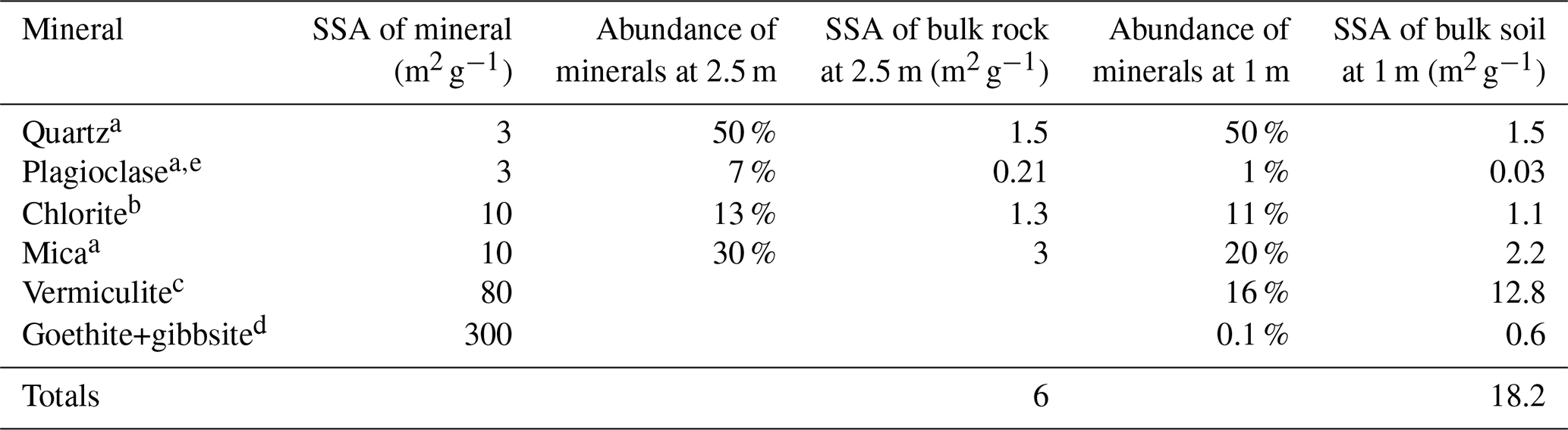
a Essington (2003). b Dogan et al. (2007) and Macht et al. (2011). c Thomas and Bohor (1969) and Kalinowski and Schweda (2007). d Borggaard (1983) and Essington (2003). e Brantley and Mellott (2000).
Our samples had <0.1 % extractable oxides generating more than half of the SSA at many depths in the top 3 m of the weathering profile. We used the weathering of an iron-bearing mica (Eq. R1) to model the potential SSA of this system. Assuming a mineral matrix comparable to our measurements in Ridge Well 1, Table 1 shows estimated SSA for each mineral identified. If we consider the minerals at 2.5 m and assume no oxidation reaction, the SSA of quartz, plagioclase, chlorite, and mica totals 6 m2 g−1. If we apply a weathering reaction that oxidizes one-third of the mica minerals to vermiculite, gibbsite, and goethite, similar to what we observe at 1 m in Ridge Well 1, we arrive at a total SSA of 18 m2 g−1 (Table 1). This model demonstrates how oxidative weathering reactions can explain the observed mineralogical and SSA profiles at our study site.
By applying SSA to assess the extent of weathering in two 21 m profiles at different landscape positions within an unglaciated schist lithology, we discovered that the morphologic boundaries within weathering profiles, namely the boundary of soil to weathered rock and the water table, did not coincide with depths where mineral SSA exhibited significant changes. Total SSA, contributed by extractable oxide (Fed) SSA and silicate SSASi, increased at depths above 3 m at both the ridge and interfluve. The weathering profiles had no other measurable change in surface area. SSA measurements enabled us to identify the depth extent of secondary phyllosilicate and iron oxide mineral formation more clearly than mineralogical methods (this paper) or geochemical mass balance methods on this variable schist bedrock (Fig. 6 and Fisher et al., 2017). Mineral SSA is thus a highly sensitive indicator of mineral production from chemical weathering.
Measuring SSA enabled us to observe the depth where nested weathering fronts generated new SSA. New SSA emerged at the same depth at both landscape positions (3 m), and new SSA was contributed by oxide minerals and secondary silicates. The initiation of oxide formation at 3 m indicates the presence of O2 penetration to at least this depth, which we identify as a weathering front. In contrast, weathering due to CO2 and acidity did not generate new SSA and extended deep into the weathering profiles, to 10 m in Ridge Well 1 and at 7 m in Interfluve Well 2 (Fisher et al., 2017). The penetration depth of O2 and the chemical and biological process associated with oxygen was a control that determined the depth of secondary mineral production for both oxide and silicate in this weathering study. This result demonstrates that element depletion profiles, which are ubiquitous in weathering studies, are not able to identify the full set of processes that occur in weathering profiles.
Future weathering studies could test the hypothesis that O2 is the limiting weathering reagent for the production of secondary oxide and phyllosilicate minerals as well as SSA via oxidation of iron in primary minerals. We arrive at this conclusion from (1) our observation of a strong positive correlation between iron oxide (Fed) SSA and silicate SSASi in the upper 3 m (Fig. 4); (2) the negative correlation of CO2 and O2 as geochemical weathering agents throughout the biogeochemical literature, at least to the depth of buffering capacity, where present (i.e., O2 for iron oxides and carbonic acid from elevated pCO2 for phyllosilicates); (3) the ubiquitous trend of decreasing subsurface gas O2 with depth to concentrations near zero at the depth where iron oxides appear and reduced iron minerals such as pyrite disappear throughout the biogeochemical literature; and (4) the typical trend of increasing subsurface pCO2 with depth to concentrations that are typically 1–2 orders of magnitude higher than in the atmosphere throughout biogeochemical literature.
Measuring SSA is not currently part of the standard suite of measurements applied in weathering studies despite its usefulness in capturing many of the effects of physical and mineralogical alterations. SSA may be especially useful in highly heterogeneous bedrock, where the compositional makes mineralogical changes difficult to associate with chemical weathering. We value the continued measurement of mass change in rock-forming elements and their associated minerals as essential to weathering studies, and we offer our work as a demonstration of the utility of SSA measurements in characterizing important hydro-biogeochemical fronts within weathering profiles.
All data in this publication are available at the University of Minnesota Digital Conservancy (Fisher, 2016h).
Please contact the authors for sample access (https://app.geosamples.org/sample/igsn/IESW10006, Fisher, 2016a; https://app.geosamples.org/sample/igsn/IESW10007, Fisher, 2016b; https://app.geosamples.org/sample/igsn/IESW10001, Fisher, 2016c; https://app.geosamples.org/sample/igsn/IESW10002, Fisher, 2016d; https://app.geosamples.org/sample/igsn/IESW10003, Fisher, 2016e; https://app.geosamples.org/sample/igsn/IESW10004, Fisher, 2016f; https://app.geosamples.org/sample/igsn/IESW10005, Fisher, 2016g). Samples are archived at Stroud Water Research Center (soil), University of Minnesota (drill core), and Minnesota State University, Mankato (pulverized soil and drill cores).
The supplement related to this article is available online at: https://doi.org/10.5194/esurf-11-51-2023-supplement.
BAF was the lead author of this article and led the Rotosonic drilling, soil sampling, specific surface area analysis, bulk density analysis, XRD mineralogy (bulk and clay), and extraction chemistry. KY was the PhD advisor for BAF, and he co-authored the funding efforts for this work, trained and assisted BAF in data collection, analysis, and interpretation, and provided significant feedback on the article contents. AKA co-authored the funding efforts for this work, co-led the Rotosonic drilling and soil sampling, and provided substantial contributions to the paper narrative and data interpretation. EAN provided extensive training on XRD procedures and assisted with XRD data interpretation. JMF provided training on iron mineralogy procedures and data interpretation. JEN graciously volunteered his time and led a group of students through the acquisition, analysis, and interpretation of the MASW data specifically with the aim of understanding this weathering profile; JEN also provided a thoughtful review of several versions of this paper.
The contact author has declared that none of the authors has any competing interests.
Publisher's note: Copernicus Publications remains neutral with regard to jurisdictional claims in published maps and institutional affiliations.
We would like to thank Brandywine Conservancy, Phoebe Fisher, and the field team at Stroud Water Research Center, especially Dave Montgomery and Shannon Hicks, for immeasurable assistance with the field component of this project. We thank Nicolas Jelinski for assistance with laser particle size analysis. We wish to thank Michael Manno and the UMN Characterization Facility for training and assistance with X-ray diffraction. Beth A. Fisher would like to express appreciation for the abundant laboratory assistance of Marta Behling Roser, Justene Davis, and Alex Durr.
This research has been supported by the National Science Foundation Christina River Basin Critical Zone Observatory (grant nos. 0724971 and 1331856).
This paper was edited by Edward Tipper and reviewed by Sétareh Rad and one anonymous referee.
Aburto, F. and Southard, R.: Refined Geomorphologic Interpretation of Glacial Deposits using Combined Soil Development Indices and LiDAR Terrain Analysis, Soil Sci. Soc. Am. J., 81, 109–123, https://doi.org/10.2136/sssaj2016.07.0211, 2017.
Anderson, S. P., Dietrich, W. E., and Brimhall, G. H.: Weathering profiles, mass-balance analysis, and rates of solute loss: Linkages between weathering and erosion in a small, steep catchment, Bull. Geol. Soc. Am., 114, 1143–1158, 2002.
Bazilevskaya, E., Lebedeva, M., Pavich, M., Rother, G., Parkinson, D. Y., Cole, D., and Brantley, S. L.: Where fast weathering creates thin regolith and slow weathering creates thick regolith, Earth Surf. Proc. Land., 38, 847–858, https://doi.org/10.1002/esp.3369, 2013.
Bazilevskaya, E., Rother, G., Mildner, D. F. R., Pavich, M., Cole, D., Bhatt, M. P., Jin, L., Steefel, C. I., and Brantley, S. L.: How Oxidation and Dissolution in Diabase and Granite Control Porosity during Weathering, Soil Sci. Soc. Am. J., 79, 55, https://doi.org/10.2136/sssaj2014.04.0135, 2014.
Blackmer, G. C.: Bedrock geology of the Coatesville quadrangle, Chester County, Pennsylvania, Pennsylvania Geological Survey, 4th ser., 2004.
Borggaard, O. K.: Effects of surface area and mineralogy of iron oxides on their surface charge and anion-adsorption properties, Clay. Clay Miner., 31, 230–232, https://doi.org/10.1346/CCMN.1983.0310309, 1983.
Brantley, S. L. and Lebedeva, M. I.: Relating land surface, water table, and weathering fronts with a conceptual valve model for headwater catchments, Hydrol. Process., 35, e14010, https://doi.org/10.1002/hyp.14010, 2021.
Brantley, S. L. and Mellott, N. P.: Surface Area and Porosity of Primary Silicate Minerals, Am. Mineral., 85, 1767–1783, 2000.
Brantley, S. L. and Olsen, A. A.: Reaction Kinetics of Primary Rock- Forming Minerals under Ambient Conditions, chap. 7.3, in: Treatise on Geochemistry (Second Edition), edited by: Holland, H. D. and Turekian, K. K., Elsevier, Oxford, 69–113, https://doi.org/10.1016/B978-0-08-095975-7.00503-9, 2014.
Brantley, S. L., Goldhaber, M. B., and Ragnarsdottir, K. V.: Crossing Disciplines and Scales to Understand the Critical Zone, Elements, 3, 307–314, https://doi.org/10.2113/gselements.3.5.307, 2007.
Brantley, S. L., Holleran, M. E., Jin, L., and Bazilevskaya, E.: Probing deep weathering in the Shale Hills Critical Zone Observatory, Pennsylvania (USA): the hypothesis of nested chemical reaction fronts in the subsurface, Earth Surf. Proc. Land., 38, 1280–1298, https://doi.org/10.1002/esp.3415, 2013a.
Brantley, S. L., Lebedeva, M., and Bazilevskaya, E.: Relating Weathering Fronts for Acid Neutralization and Oxidation to pCO2 and pO2, in: Treatise on Geochemistry: Second Edition, vol. 6, Elsevier Inc., 327–352, https://doi.org/10.1016/B978-0-08-095975-7.01317-6, 2013b.
Brimhall, G. H. and Dietrich, W. E.: Constitutive mass balance relations between chemical composition, volume, density, porosity, and strain in metasomatic hydrochemcal systems: Results on weathering and pedogenesis, Geochim. Cosmochim. Ac., 51, 567–587, https://doi.org/10.1016/0016-7037(87)90070-6, 1987.
Brunauer, S., Emmett, P. H., and Teller, E.: Adsorption of Gases in Multimolecular Layers, J. Am. Chem. Soc., 60, 309–319, https://doi.org/10.1021/ja01269a023, 1938.
Burt, R.: Soil Survey Laboratory Methods Manual, Soil Survey Investigations Report, 42, 735, https://doi.org/10.1021/ol049448l, 2004.
Burt, R. and Staff, S. S. (Eds.): Kellogg Soil Survey Laboratory Methods Manual, Soil Survey Investigations Report no. 42, Version 5, USDA – Natural Resources Conservation Service, 1003 pp., 2014.
Buss, H. L., Sak, P. B., Webb, S. M., and Brantley, S. L.: Weathering of the Rio Blanco quartz diorite, Luquillo Mountains, Puerto Rico: Coupling oxidation, dissolution, and fracturing, Geochim. Cosmochim. Ac., 72, 4488–4507, 2008.
Carter, B. J. and Ciolkosz, E. J.: Sorting and thickness of waste mantle material on a sandstone spur in central Pennsylvania, Catena, 13, 241–256, https://doi.org/10.1016/0341-8162(86)90001-9, 1986.
Clarke, B. A. and Burbank, D. W.: Bedrock fracturing, threshold hillslopes, and limits to the magnitude of bedrock landslides, Earth Planet. Sc. Lett., 297, 577–586, https://doi.org/10.1016/j.epsl.2010.07.011, 2010.
Dogan, M., Dogan, A. U., Yesilyurt, F. I., Alaygut, D., Buckner, I., and Wurster, D. E.: Baseline studies of The Clay Minerals Society special clays: specific surface area by the Brunauer Emmett Teller (BET) method, Clay. Clay Miner., 55, 534–541, https://doi.org/10.1346/CCMN.2007.0550508, 2007.
Dunlop, D. J. and Ozdemir, O.: Magnetizations in Rocks and Minerals, in: Treatise on Geophysics: Geomagnetism, edited by: Kono, M., Elsevier, Amsterdam, 227–336, https://doi.org/10.1016/B978-044452748-6.00093-6, 2007.
Eberl, D. D.: User's Guide to RockJock – A Program for Determining Quantitative Mineralogy From Powder X-Ray Diffraction Data, U. S. Geological Survey Open-File Report 03-78, 1–47, 2003.
Eppinger, B. J., Hayes, J. L., Carr, B. J., Moon, S., Cosans, C. L., Holbrook, W. S., Harman, C. J., and Plante, Z. T.: Quantifying Depth-Dependent Seismic Anisotropy in the Critical Zone Enhanced by Weathering of a Piedmont Schist, J. Geophys. Res.-Earth, 126, e2021JF006289, https://doi.org/10.1029/2021JF006289, 2021.
Essington, M.: Soil and Water Chemistry: An Integrative Approach, 1st edn., CRC Press, Boca Raton, 534 pp., https://doi.org/10.1201/b12397, 2003.
Eusterhues, K., Rumpel, C., and Kogel-Knabner, I.: Organo-mineral associations in sandy acid forest soils: importance of specific surface area, iron oxides and micropores, Eur. J. Soil Sci., 56, 753–763, https://doi.org/10.1111/j.1365-2389.2005.00710.x, 2005.
Fisher, B.: LP_Well01, University of Minnesota-Twin Cities [sample], https://app.geosamples.org/sample/igsn/IESW10006, 2016a.
Fisher, B.: LP_Well02, University of Minnesota-Twin Cities [sample], https://app.geosamples.org/sample/igsn/IESW10007, 2016b.
Fisher, B.: LP_Pit_For1, University of Minnesota-Twin Cities [sample], https://app.geosamples.org/sample/igsn/IESW10001, 2016c.
Fisher, B.: LP_Pit_For2, University of Minnesota-Twin Cities [sample], https://app.geosamples.org/sample/igsn/IESW10002, 2016d.
Fisher, B.: LP_Pit_For3, University of Minnesota-Twin Cities [sample], https://app.geosamples.org/sample/igsn/IESW10003, 2016e.
Fisher, B.: LP_Pit_For5, University of Minnesota-Twin Cities [sample], https://app.geosamples.org/sample/igsn/IESW10004, 2016f.
Fisher, B.: LP_Pit_For6, University of Minnesota-Twin Cities [sample], https://app.geosamples.org/sample/igsn/IESW10005, 2016g.
Fisher, B.: Geomorphic controls on mineral weathering, elemental transport, carbon cycling, and production of mineral surface area in a schist bedrock weathering profile, Piedmont Pennsylvania, University of Minnesota, http://hdl.handle.net/11299/183377 (last access: 11 November 2016), 2016h.
Fisher, B. A., Rendahl, A. K., Aufdenkampe, A. K., and Yoo, K.: Quantifying weathering on variable rocks, an extension of geochemical mass balance: Critical zone and landscape evolution, Earth Surf. Proc. Land., 42, 2457–2468, https://doi.org/10.1002/esp.4212, 2017.
Fisher, B. A., Aufdenkampe, A. K., Yoo, K., Aalto, R. E., and Marquard, J.: Soil carbon redistribution and organo-mineral associations after lateral soil movement and mixing in a first-order forest watershed, Geoderma, 319, 142–155, https://doi.org/10.1016/j.geoderma.2018.01.006, 2018.
Graham, R., Rossi, A., and Hubbert, R.: Rock to regolith conversion: Producing hospitable substrates for terrestrial ecosystems, GSA Today, 20, 4–9, https://doi.org/10.1130/GSAT57A.1, 2010.
Gu, X., Rempe, D. M., Dietrich, W. E., West, A. J., Lin, T. C., Jin, L., and Brantley, S. L.: Chemical reactions, porosity, and microfracturing in shale during weathering: The effect of erosion rate, Geochim. Cosmochim. Ac., 269, 63–100, https://doi.org/10.1016/j.gca.2019.09.044, 2020.
Hasenmueller, E. A., Jin, L., Stinchcomb, G. E., Lin, H., Brantley, S. L., and Kaye, J. P.: Topographic controls on the depth distribution of soil CO2 in a small temperate watershed, Appl. Geochem., 63, 58–69, https://doi.org/10.1016/j.apgeochem.2015.07.005, 2015.
Holmgren, G.: A rapid citrate-dithionite extractable iron procedure, Soil Sci. Soc. Am. J., 31, 210–211, https://doi.org/10.2136/sssaj1967.03615995003100020020x, 1967.
Hunt, C. P., Singer, M. J., Kletetschka, G., TenPas, J., and Verosub, K. L.: Effect of citrate-bicarbonate-dithionite treatment on fine-grained magnetite and maghemite, Earth Planet. Sc. Lett., 130, 87–94, https://doi.org/10.1016/0012-821X(94)00256-X, 1995.
Jackson, M. and Hseung, Y.: Weathering sequence of clay-size minerals in soils and sediments: II. Chemical weathering of layer silicates, Soil Sci. Soc. Am. J., 16, 3–6, 1952.
Jackson, M. L.: Interlaying of expansible layer sililcates in soils by chemical weathering, Clay. Clay Miner., 11, 29–46, https://doi.org/10.1346/CCMN.1962.0110104, 1963.
Jackson, M. L. and Barak, P.: Soil Chemical Analysis: Advanced Course, UW-Madison Libraries Parallel Press, 930 pp., ISBN 9781893311473, 2005.
Jackson, M. L., Tyler, S. A., Willis, A. L., Bourbeau, G. A., and Pennington, R. P.: Weathering Sequence of Clay-Size Minerals in Soils and Sediments. I. Fundamental Generalizations, J. Phys. Colloid Chem., 52, 1237–1260, https://doi.org/10.1021/j150463a015, 1948.
Jin, L., Rother, G., Cole, D. R., Mildner, D. F. R., Duffy, C. J., and Brantley, S. L.: Characterization of deep weathering and nanoporosity development in shale–A neutron study, Am. Mineral., 96, 498–512, https://doi.org/10.2138/am.2011.3598, 2011.
Jobbágy, E. G. and Jackson, R. B.: The vertical distribution of soil organic carbon and its relation to climate and vegetation, Ecol. Appl., 10, 423–436, https://doi.org/10.1890/1051-0761(2000)010[0423:TVDOSO]2.0.CO;2, 2000.
Kalinowski, B. E. and Schweda, P.: Rates and nonstoichiometry of vermiculite dissolution at 22C, Geoderma, 142, 197–209, 2007.
Keil, R. G. and Mayer, L. M.: Mineral Matrices and Organic Matter, Elsevier Ltd., 337–359, https://doi.org/10.1016/B978-0-08-095975-7.01024-X, 2014.
Keil, R. G., Mayer, L. M., Quay, P. D., Richey, J. E., and Hedges, J. I.: Loss of organic matter from riverine particles in deltas, Geochim. Cosmochim. Ac., 61, 1507–1511, https://doi.org/10.1016/S0016-7037(97)00044-6, 1997.
Kim, H., Stinchcomb, G., and Brantley, S. L.: Feedbacks among O2 and CO2 in deep soil gas, oxidation of ferrous minerals, and fractures: A hypothesis for steady-state regolith thickness, Earth Planet. Sc. Lett., 460, 29–40, https://doi.org/10.1016/j.epsl.2016.12.003, 2017.
Knauss, K. G. and Thomas, J. W.: Muscovite dissolution kinetics as a function of pH and time at 70C, Geochim. Cosmochim. Ac., 53, 1493–1501, 1989.
Lesley, J. P.: The iron manufacturer's guide to the furnaces, forges and rolling mills of the United States: With maps and plates, Wiley, New York, 772 pp., ISBN 9780608414218, 1859.
Liptzin, D., Silver, W. L., and Detto, M.: Temporal dynamics in soil oxygen and greenhouse gases in two humid tropical forests, Ecosystems, 14, 171–182, https://doi.org/10.1007/s10021-010-9402-x, 2011.
Lowrie, W.: Fundamentals of Geophysics, Cambridge University Press, 354 pp., ISBN 9780521467285, 1997.
Macht, F., Eusterhues, K., Pronk, G. J., and Totsche, K. U.: Specific surface area of clay minerals: Comparison between atomic force microscopy measurements and bulk-gas (N2) and -liquid (EGME) adsorption methods, Appl. Clay Sci., 53, 20–26, https://doi.org/10.1016/j.clay.2011.04.006, 2011.
Maher, K.: The dependence of chemical weathering rates on fluid residence time, Earth Planet. Sc. Lett., 294, 101–110, https://doi.org/10.1016/j.epsl.2010.03.010, 2010.
Maxbauer, D. P., Feinberg, J. M., Fox, D. L., and Clyde, W. C.: Magnetic minerals as recorders of weathering, diagenesis, and paleoclimate: A core–outcrop comparison of Paleocene–Eocene paleosols in the Bighorn Basin, WY, USA, Earth Planet. Sc. Lett., 452, 15–26, https://doi.org/10.1016/j.epsl.2016.07.029, 2016.
Mayer, L. M. and Xing, B.: Organic Matter – Surface Area Relationships in Acid Soils, Soil Sci. Soc. Am. J., 65, 567–571, https://doi.org/10.2136/sssaj2001.651250x, 2001.
Merritts, D. J. and Rahnis, M. A.: Pleistocene Periglacial Processes and Landforms, Mid-Atlantic Region, Eastern United States, https://doi.org/10.1146/annurev-earth-032320-102849, 2022.
Moore, D. M. and Reynolds, R. C.: X-ray diffraction and the identification and analysis of clay minerals, Oxford University Press, 378 pp., ISBN 9780195087130, 1997.
Muggeo, V. M. R.: segmented: An R package to Fit Regression Models with Broken-Line Relationships, R News, 8, 20–25, 2008.
NRCS: Soil Survey Manual, Soil Conservation Service, U. S. Department of Agriculture Handbook, 18, 1–2, https://doi.org/10.1097/00010694-195112000-00022, 1993.
Official Soil Series Descriptions. Natural Resources Conservation Service, United States Department of Agriculture: https://soilseries.sc.egov.usda.gov/OSD_Docs/M/MANOR.html, last access: 30 May 2012.
Parsekian, A. D., Singha, K., Minsley, B. J., Holbrook, W. S., and Slater, L.: Multiscale geophysical imaging of the critical zone, Rev. Geophys., 53, 1–26, https://doi.org/10.1002/2014RG000465, 2015.
Pawlik, Ł., Phillips, J. D., and Šamonil, P.: Roots, rock, and regolith: Biomechanical and biochemical weathering by trees and its impact on hillslopes – A critical literature review, Earth-Sci. Rev., 159, 142–159, https://doi.org/10.1016/j.earscirev.2016.06.002, 2016.
Pedrazas, M. A., Hahm, W. J., Huang, M. H., Dralle, D., Nelson, M. D., Breunig, R. E., Fauria, K. E., Bryk, A. B., Dietrich, W. E., and Rempe, D. M.: The Relationship Between Topography, Bedrock Weathering, and Water Storage Across a Sequence of Ridges and Valleys, J. Geophys. Res.-Earth, 126, e2020JF005848, https://doi.org/10.1029/2020JF005848, 2021.
Pope, G. A.: Regolith and Weathering (Rock Decay) in the Critical Zone, chap. 4, in: Developments in Earth Surface Processes, vol. 19, edited by: Giardino, J. R. and Houser, C., Elsevier, 113–145, https://doi.org/10.1016/B978-0-444-63369-9.00004-5, 2015.
Poppe, L. J., Paskevich, V. F., Hathaway, J. C., and Blackwood, D. S.: A laboratory manual for X-ray powder diffraction, Open-File Report, https://doi.org/10.3133/ofr0141, 2001.
Prentice, I. C., Bartlein, P. J., and Webb III, T.: Vegetation and climate change in Eastern North America since the last glacial maximum, Ecology, 72, 2038–2056, 1991.
Rempe, D. M. and Dietrich, W. E.: A bottom-up control on fresh-bedrock topography under landscapes, P. Natl. Acad. Sci. USA, 111, 6576–6581, https://doi.org/10.1073/pnas.1404763111, 2014.
Richardson, D. C., Newbold, J. D., Aufdenkampe, A. K., Taylor, P. G., and Kaplan, L. A.: Measuring heterotrophic respiration rates of suspended particulate organic carbon from stream ecosystems, Limnol. Oceanogr.-Meth., 11, 247–261, 2013.
Richter, D. de B. and Billings, S. A.: “One physical system”: Tansley's ecosystem as Earth's critical zone, New Phytol., 206, 900–912, https://doi.org/10.1111/nph.13338, 2015.
Riebe, C. S., Hahm, W. J., and Brantley, S. L.: Controls on deep critical zone architecture: a historical review and four testable hypotheses, Earth Surf. Proc. Land., 42, 128–156, https://doi.org/10.1002/esp.4052, 2017.
Righi, D., Petit, S., and Bouchet, A.: Characterization of Hydroxy-Interlayered Vermiculite and Illite/Smectite Interstratified Minerals from the Weathering of Chlorite in a Cryorthod, Clays Clay Miner., 41, 484–495, https://doi.org/10.1346/CCMN.1993.0410409, 1993.
Ross, G. J. and Kodama, H.: Experimental alteration of a chlorite into a regularly interstratified chlorite-vermiculite by chemical oxidation, Clay. Clay Miner., 24, 183–190, 1976.
Schoeneberger, P. J., Wysocki, D. A., Benham, E. C., and Soil Survey Staff: Field Book for Describing and Sampling Soils, Version 3.0. Natural Resources Conservation Service, National Soil Survey Center, Lincoln, NE, ISBN 9780160915420, 2012.
Shang, C. and Zelazny, L. W.: Selective dissolution techniques for mineral analysis of soils and sediments, Methods of Soil Analysis. Part 5. Mineralogical Methods, SSSA Book Series, https://doi.org/10.2136/sssabookser5.5.c3, 2008.
Shields, D. and Benson, B.: Catalyst for Conservation: the Brandywine Conservancy's success in saving King Ranch lands in Pennsylvania, 1st edn., Pemcor Printing, LLC, USA, 112 pp., ISBN 9780979587252, 2011.
Stinchcomb, G. E., Kim, H., Hasenmueller, E. A., Sullivan, P. L., Sak, P. B., and Brantley, S. L.: Relating soil gas to weathering using rock and regolith geochemistry, Am. J. Sci., 318, 727–763, https://doi.org/10.2475/07.2018.01, 2018.
Thomas, J. and Bohor, B. F.: Surface area of vermiculite with nitrogen and carbon dioxide as adsorbates, Clay. Clay Miner., 17, 205–209, https://doi.org/10.1346/CCMN.1969.0170403, 1969.
Thompson, A., Rancourt, D. G., Chadwick, O. A., and Chorover, J.: Iron solid-phase differentiation along a redox gradient in basaltic soils, Geochim. Cosmochim. Ac., 75, 119–133, https://doi.org/10.1016/j.gca.2010.10.005, 2011.
White, A. F. and Buss, H. L.: Natural Weathering Rates of Silicate Minerals, in: Treatise on Geochemistry, edited by: Turekian, K. K. and Holland, H. D., Elsevier, 115–155, https://doi.org/10.1016/B978-0-08-095975-7.00504-0, 2014.
White, A. F., Blum, A. E., Schulz, M. S., Bullen, T. D., Harden, J. W., and Peterson, M. L.: Chemical weathering rates of a soil chronosequence on granitic alluvium: I. Quantification of mineralogical and surface area changes and calculation of primary silicate reaction rates, Geochim. Cosmochim. Ac., 60, 2533–2550, https://doi.org/10.1016/0016-7037(96)00106-8, 1996.
Wilson, M. A., Indorante, S. J., Lee, B. D., Follmer, L. R., Williams, D. R., Fitch, B. C., McCauley, W. M., Bathgate, J. D., and Kabrick, J. M.: Soil Geochemistry of Loess Landscapes, Shawnee Hills, Southern Illinois, United States, Soil Sci. Soc. Am. J., 77, 1269–1283, https://doi.org/10.2136/sssaj2013.02.0051, 2013.