Testing the sensitivity of the CAESAR-Lisflood landscape evolution model to grid cell size

Landscape evolution models (LEMs) are useful for understanding how large-scale processes and perturbations influence the development of the surface of the Earth and other planets. With their increasing sophistication and improvements in computational power, they are finding greater uptake in analyses at finer spatial and temporal scales. For many LEMs, the land surface is represented by a grid of regularly spaced and sized grid cells, or pixels, referred to as a digital elevation model (DEM), yet despite the importance of the DEM to LEM studies, there has been little work to understand the influence of grid cell size (i.e. resolution) on model behaviour. This is despite the choice of grid cell size being arbitrary for many studies, with users needing to balance detail with computational efficiency. Using the Morris method (MM) for global sensitivity analysis, the sensitivity of the CAESAR-Lisflood LEM to the grid cell size is evaluated relative to a set of influential user-defined parameters, showing that it had a similar level of influence as a key hydrological parameter and the choice of sediment transport law. Outputs relating to discharge and sediment yields remained stable across different grid cell sizes until the cells became so large that the representation of the hydrological network degraded. Although total sediment yields remained steady when changing the grid cell sizes, closer analysis revealed that using a coarser grid resulted in it being built up from fewer yet more geomorphically active events, risking outputs that are “the right answer but for the wrong reasons”. These results are important considerations for modellers using LEMs and the methodologies detailed provide solutions to understanding the impacts of modelling choices on outputs.

1 Introduction

Landscape evolution models (LEMs) simulate the morphodynamic change of landscapes typically over long timescales ranging from decades to multi-millennia (van der Beek, 2013). Whilst LEMs were predominantly developed for experimental purposes, such as to understand broad-scale basin behaviour over long timescales, the increasing sophistication of the models ushered in an era of “second-generation” LEMs (Coulthard et al., 2013). This has seen an increase in the use of LEMs over shorter time frames with smaller grid cell sizes for operational purposes or to support decision-making (e.g. Environment Agency, 2021; Feeney et al., 2022; Ramirez et al., 2022; Wong et al., 2021). This operationalisation of LEMs brings with it a need to understand model limitations and uncertainties that may have a bearing over real-world decisions.

Landscape change is often simulated by applying process-based rules of hydrology, erosion, and deposition to change the elevation of cells in a regular grid, or in an irregular mesh, that represents the land surface. The spatial resolution of this virtual surface is an important consideration due to two contrasting effects. Firstly, if it is too coarse (e.g. larger grid cells), it may smooth out the terrain too much and miss out key landscape features. Secondly, a finer or higher spatial resolution will better represent features but increases the number of cells and points for the area simulated that in turn increases the computation time (halving the grid cell size results in a square increase in the number of grid cells). Therefore, where high-resolution data are available, a compromise digital elevation model (DEM) grid cell size is used by LEMs that captures drainage basin and hillslope features whilst maintaining a low number of grid cells (Hancock, 2005; Hancock et al., 2016).

Unexpectedly, there are few studies that specifically address the impacts of grid cell resolution on LEMs. Schoorl et al. (2000) used the LAPSUS model to simulate landscape development on a series of artificial DEMs with varying grid cell sizes and showed that with larger grid cells, total erosion or sediment yield from the simulations increased due to an in increase in erosion coupled with a decrease in sedimentation. They argued that the erosion increase was due to the model parameterisation but that a coarsening in the physical representation of the landscape with larger grid cells made sedimentation more difficult, concluding that it is important that the extent of the landscape and its relief characteristics are realistically represented by the used DEM. Hancock (2006) showed a sensitivity in LEM outputs to DEMs created with different kriging/interpolation methods. These changes in the representation can then have important cumulative impacts if the landscape is modelled since LEMs may exacerbate, or deepen, concavities or other features ultimately leading to different shape topographies (Ijjasz-Vasquez et al., 1992; Willgoose et al., 2003). Hancock et al. (2016) illustrated this by perturbating a DEM by different ranges of random values and simulating millennial timescale changes on the different surfaces using the SIBERIA LEM. They found that an increasing magnitude of random surface variability did not significantly alter total basin sediment yields but greatly changed the temporal pattern or delivery of sediment output. Furthermore, after 10 000 years of simulation, the alternative positions of initial random perturbations strongly influenced local patterns of hillslope erosion and landscape evolution – although general landscape metrics were very similar. Hancock and Evans (2006) looked at two small catchments in North Australia using 10, 20, 30, 40, and 50 m grid cells to evaluate the impact of resolution in determining channel head location and the area–slope relationship as well as cumulative area distribution that is a key driver in the SIBERIA (Willgoose and Riley, 1998) LEM. Their findings showed a clear drop in the area–slope relationship with larger grid cells – largely due to the smoothing and subsequent simplification of topography. Finlayson and Montgomery (2003) show a major degradation of DEM mean slope values when resampling from 30 to 90 to 900 m – representing the smoothing of features and lowering of gradients. Finally, Pelletier (2010) noted an impact of grid cell size in LEMs where using larger grid cell flow paths can become dominated by only being able to change direction by 45 or 90^∘.

Looking outside the immediate LEM literature, with cellular morphodynamic models (similar in many ways to LEMs), Doeschl-Wilson and Ashmore (2005) examined the Murray and Paola (1994) braided river model and noted that the model performance was strongly affected by the spatial scales at which the input topography was represented. They demonstrated that when tested over a range of different spatial resolutions, the model had a “preferred” scale where it self-adjusted to have a channel width with a certain number of cells (rather than a distance represented by a number of cells) (Doeschl-Wilson and Ashmore, 2005). Possible reasons why there is a sensitivity to grid resolution in cellular approaches were discussed by Nicholas (2005), who stated that this was a consequence of the water- and sediment-routing equations used in simplified cellular models. For example, where sediment and water were routed in proportion to local bed slopes, the calculations may become sensitive to very small variations in elevation as grid cell resolution changes (Nicholas 2005), that also shows a weakness in using local bed slope to represent the energy slope. This is especially important in a LEM or morphodynamic model where these elevations will be changing every iteration in response to erosion and deposition – this effect will be amplified or reduced by grid resolution.

The two-dimensional flow of water over landscapes is a key process in LEMs and for two-dimensional hydraulic models of flood inundation, the effects of grid cell resolution have been extensively studied (e.g. Horritt and Bates, 2001; Savage et al., 2016). Horritt and Bates (2001) tested the LISFLOOD-FP inundation model against satellite-derived flood inundation extents over DEMs with grid cell resolutions ranging from 10 to 1000 m. Overall, they showed a good comparison between inundation area/extent over all resolutions (using the same model calibrations) though comparison of flood wave travel time was notably different. Interestingly, this shows how grid cell resolution was less important in spatial matches between observed and modelled water extents but certainly interfered with the equations determining where water went (travel times), in effect simplifying them to a point where they did not perform adequately with respect to resolution. Claessens et al. (2005) summarise these effects neatly: the grid cell resolution acts to firstly simplify the topographic data, and secondly, any model processes or governing equations that operate below this resolution will therefore also be simplified. This can lead to apparent gains in accuracy due to greater process representation within the model being countered by the coarser model resolution (Claessens et al., 2005). Horritt and Bates (2001) also described how changes in topographic detail with different resolution DEMs also affected floodplain storage. Similar topographic degradation affecting model behaviour was observed by Savage et al. (2016), who noted that when using LISFLOOD-FP to simulate inundation over a wide range of resolutions, model performance degraded where grid cells were larger than 50 m. This was due to the channel being poorly represented within the DEM leading to increased floodplain water depths – lower velocities that all affected model performance negatively. Importantly, Savage et al. (2016) also observed how model resolution affected parameter sensitivity, a secondary effect aside from model performance. This was also a key finding of Lim and Brandt (2019) using the hydraulic component of CAESAR-Lisflood LEM to examine any dependency between DEM resolution, Manning's n roughness coefficient, and model performance. Comparing model inundation extents and depths for flood events on two rivers to simulation results over grid cell resolutions from 1–50 m, they demonstrated that high-resolution DEMs performed better with higher Manning's n values, whereas lower n values gave better outputs for lower-resolution DEMs. Lim and Brandt (2019) also showed that whilst coarser-resolution DEMs generated better value performances according to their metrics, there were more discrepancies between known flooding and predicted water surface elevations, illustrating a dependency on the metric used for assessment. Choice of metric for assessing model performance is also an important issue presently facing LEM studies, with metrics based on catchment outputs displaying different behaviours to those derived from changes within the catchment (Skinner et al., 2018).

In computational fluid dynamics (CFD), where more complex numerical methods are used for hydraulic modelling, the effects of different grid resolutions or meshing methods are widely considered. Where CFD model simulations are applied to engineering solutions, there are controls and standards for the verification of models (Vassiliadis et al., 2001) that are also reflected in the journal publication policies such as “Solutions over a range of significantly different grid resolutions should be presented to demonstrate grid independent or grid convergent results” (Roache, 2019; Roache et al., 1986). Here, grid independent (or grid independence) refers to whether errors or differences between different resolution simulations are sufficiently small. Hardy et al. (2003) provide a clear summary and example of methods for assessing grid independence using a “Grid Convergence Index approach”. Nicholas (2005) comments that whilst grid independence is considered a key requirement of computational fluid dynamics (CFD) approaches – it may not be reasonable to use such approaches in cellular methods. A logical step might be to use methods from CFD grid independence testing on LEMs. However, grid independence tests are largely performed during steady flow conditions (e.g. Hardy et al., 2003), measuring flow velocities in x, y, and z directions (for example), but sediment processes in LEMs and morphodynamic models are highly episodic and non-linear, even when averaged over medium timescales (Coulthard et al., 1998; Coulthard and Van De Wiel, 2012). Therefore, the availability and choice of metrics to assess LEM performance is difficult.

This issue of which metrics to use to assess LEM performance was considered by Skinner et al. (2018) when they carried out a multidimensional sensitivity analysis on the CAESAR-Lisflood (Coulthard et al., 2013) LEM. Previously, such studies have been hampered by long model run times, making Monte Carlo style analyses difficult; but here, Skinner et al. (2018) used the Morris method (MM; Morris, 1991) to analyse the sensitivity of 15 different model parameters on model performance. Key to this study was the assessment of model behaviours across 15 model functions across 4 core behaviour groups: catchment sediment yields, internal geomorphology, catchment discharge, and model efficiency. The work of Skinner et al. (2018) also provides a framework within which we could look at the impact of grid cell size on both overall model performance and in relation to the other model parameters tested, in effect providing us with a way of making a comprehensive assessment of the impact of grid cell size on LEM performance.

It is clear from the literature that small changes in the landscape (as represented by DEMs) can have an impact on LEM outputs. As the spatial resolution of a DEM affects the representation of topographic features, resolution will have an impact on model performance and output. LEMs may be especially sensitive to this as they typically use local gradients to determine erosion and deposition, thus potentially generating a positive feedback if erosion and deposition increases local changes. In this paper, we address these issues above by using the CAESAR-Lisflood LEM to simulate erosion and deposition over a wide range of grid cell sizes. Output metrics representing geomorphic, hydrological, and model performance are then assessed using the Morris method to establish how grid cell size affects model results and performance, and importantly, whether there are any parameter sensitivities to these resolutions. Our aim is to understand how user choice of grid resolution might influence outputs with an operational use of the model, which has influenced our choice of catchment and timescales simulated.

2 Methods

2.1 Study catchment and DEM data

The model tests were carried out on a DEM of Tin Camp Creek in the Northern Territory, Australia (see Fig. 1). Tin Camp Creek has a catchment area of 0.5 km² and is located within a tropical climate where its watercourse is ephemeral – rainfall in the wet season features small, intense convective events. It is a small sub-catchment of the wider Tin Camp Creek system and has been used previously for studies using LEMs (Hancock et al., 2010; Hancock, 2006, 2012; Skinner et al., 2018). The DEM used is produced from high-resolution digital photogrammetry and available at 2 m grid resolution at its finest (as described by Hancock, 2012). For this study, the 2 m DEM was resampled using the Raster Resample tool in ArcMap v10.4.1 to grid cell sizes between 2 and 30 m at 2 m iterations and a final 50 m grid resolution. The choice of small area DEM is deliberate to reduce model run times – especially when using the smallest grid cell sizes. The 2 m resolution proved to be too computationally expensive so was not used.

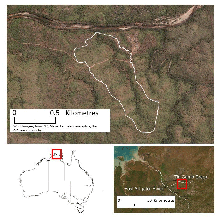
Figure 1 Location of the Tin Camp Creek study site (Imagery source: World imagery from Esri, Maxar, Earthstar Geographics, and the GIS User Community).

2.2 The CAESAR-Lisflood model

The LEM used was the CAESAR-Lisflood model (Coulthard et al., 2013). A full description of the CAESAR-Lisflood model can be found in Coulthard et al. (2013), and its core functionality is only summarised here. The model utilises an initial DEM built from a regular grid of cells, and in the catchment mode (as used in this model setup), it is driven by a rainfall time series that can be lumped or spatially distributed (Coulthard and Skinner, 2016). At each time step, the rainfall input is converted to surface runoff using TOPMODEL (Beven and Kirkby, 1979), where the rate and magnitude of conversion is largely controlled by a key parameter “m”. Surface runoff is then distributed across the catchment and routed across the DEM using the LISFLOOD-FP component (Bates et al., 2010). LISFLOOD-FP uses a simple finite volume method to determine flow between cells (Manhattan neighbours) based on the water surface gradient and the surface friction (Manning's n) with a dynamic time step controlled by a Courant condition (determined by flow depth and velocity). A key improvement of LISFLOOD-FP post 2010 (Bates et al., 2010) is the simple incorporation of inertia based on fluxes between cells in the previous time step. Including inertia significantly reduces numerical instability in the solution, also allowing larger flow model time steps to be used. The CAESAR component of the model drives the landscape development using sediment transport formulae based on flow depths and velocities derived from the LISFLOOD-FP component. Three sediment transport formulae are incorporated within CAESAR-Lisflood, all with different approaches: firstly, the Wilcock and Crowe (2003) approach, which incorporates a “hiding function” to represent how a sand fraction in gravel beds reduces gravel sediment transport below certain flow thresholds; second, the Einstein (1950) formulation that takes a probabilistic approach to whether or not sediment is entrained; third, the Meyer-Peter and Müller approach (Meyer-Peter and Müller, 1948) that takes a more typical approach to sediment transport where it is directly related to the flow properties. All three sediment transport formulae are chosen for CAESAR-Lisflood since, unlike many other methods, they calculate sediment transport for individual size fractions which is a key requirement for the operation of the model with different grain sizes as explained below. Bed load is distributed to neighbouring cells proportionally based on relative bed elevations. This study has not used the suspended sediment processes in the model. The model can handle nine different grain sizes, and information is stored in surface and sub-surface layers where only the top surface layer is “active” for erosion and deposition. A comprehensive description of this process can be found in Van De Wiel et al. (2007). The model has capability for bedrock erosion but the setup for this study does not include a representation of bedrock and is unlikely to be influential over the 30-year operational time frame used. An initial soil layer is determined globally using the information within the grain size set parameter (see Table 1).

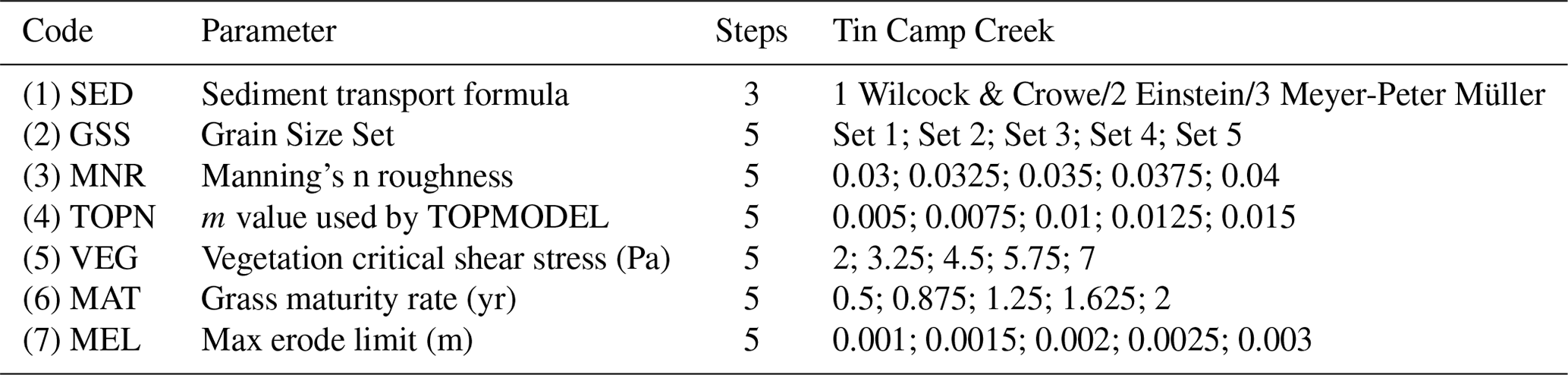
Table 1 Parameters selected for the MM test, the number of iterative steps applied, and the values used for each iterative step. A description of the role of these parameters within the model is provided in Appendix A.

CAESAR-Lisflood is freely available and since 1996 there have been 119 published studies using the model over a wide range of temporal and spatial scales (Skinner and Coulthard, 2022). Here we used CAESAR-Lisflood v1.9 with modifications to allow it to run in batch mode and to automatically collect information relevant to the behavioural functions (outlined below).

2.3 Morris method

Our study used the Morris method (MM) described in Ziliani et al. (2013), i.e. the original MM of Morris (1991), as extended by Campolongo et al. (2007), and applied the “sensitivity” package in the R statistical environment (Pujol, 2008) to generate the parameter sets for the sensitivity analysis (SA). To set up the MM, we selected a number of parameters to be assessed, specifying a minimum and maximum range for each, plus a number of iterative steps. The parameter values are equally spaced based on the range and number of steps – for example, a parameter with a range of 2 to 10 and 5 incremental steps would have available values of 2, 4, 6, 8, and 10. This was carried out for each parameter and where possible, the same number of incremental steps were used for each. For a full description of the MM applied to CAESAR-Lisflood, see Skinner et al. (2018), and a summary is provided below.

The MM uses a system of repeats to sample the global parameter space. For each parameter, the user defines minimum and maximum values and the number of incremental steps within that range from which to choose values (e.g. with a minimum value of 2, a maximum value of 10, and five incremental steps, the values of 2, 4, 6, 8, and 10 would be available). The first test in each repeat uses a randomly selected set of parameters determined from the whole available parameter space. The second test in the repeat uses the same parameter set yet varies a single randomly determined parameter to a different randomly determined value from those available. That parameter would then be excluded from selection for change for the rest of this repeat, with the process continuing until all parameters have been changed once.

The sensitivity of the model to changes in parameter values is evaluated by the changes of objective function values between sequential tests within repeats, relative to the number of incremental steps the parameter value has been changed by (e.g. for the set of values 2, 4, 6, 8, and 10, a switch from an initial value of 4 to either 2 or 6 is one step, a change to 8 is two steps, and 10 is three). The change in objective function score between two sequential tests divided by the number of incremental step changes is an elementary effect (EE) of that objective function and the parameter changed (Eq. 1). After all tests for each grid resolution have been performed, the main effect (ME) for each objective function and parameter is calculated from the mean of the relevant EEs – the higher the ME, the greater the model's sensitivity. Alongside the ME, the standard deviation of the EEs is also calculated as this provides an indication of the non-linearity within the model.

$$\begin{array}{}\text{(1)}& \begin{array}{rl}& d_{ij}=\\ & \left|{\displaystyle \frac{y\left(x_{\mathrm{1}},x_{\mathrm{2}}\mathrm{\dots },x_{i-\mathrm{1}},x_i+{\mathrm{\Delta }}_i,x_{i+\mathrm{1}},\mathrm{\dots },x_k\right)-y\left(x_{\mathrm{1}},x_{\mathrm{2}},\mathrm{\dots },x_{i-\mathrm{1}},x_i,x_{i+\mathrm{1}},\mathrm{\dots },x_k\right)}{{\mathrm{\Delta }}_i}}\right|\end{array},\end{array}$$

where d_ij is the value of the jth EE (j=1, …, r; where r is the number of repetitions (here r=100)) of the ith parameter (e.g. i=1 refers to sediment transport formula; see Table 1), x_i is the value of the ith parameter, k is the number of parameters investigated (here 7), $y(x_{\mathrm{1}},x_{\mathrm{2}},\mathrm{\dots },x_k)$ is the value of the selected objective function, and Δ_i is the change in incremental steps that parameter i was altered by.

In Skinner et al. (2018), an MM test was applied to a DEM of the same Tin Camp Creek basin used for this study, using a single 10 m grid cell size. That test used a sub-set of 15 parameters and 100 repeats, producing 1600 tests in total. Here, we are testing 15 different resolutions so the same level of scrutiny of parameters and repeats would result in 24 000 tests to be required. To reduce the computational expense, we reduced the 15 parameters to the 7 that exhibited the greatest impacts on model behaviour in Skinner et al. (2018). In addition, the number of repeats was reduced to 10, in line with the minimum number suggested by Ziliani et al. (2013). This reduced the total number of tests to 80 for each DEM resolution and 1200 in total. The only difference in the parameter value ranges to Skinner et al. (2018) is the inclusion of Meyer-Peter and Müller (1948) as an additional sediment transport law, with changes between any of the sediment transport laws being counted as a single iterative step change. The parameters and their values are shown in Table 1.

Table 2 Core behaviours of the model and the model functions adopted to assess changes to these (from Skinner et al., 2018).

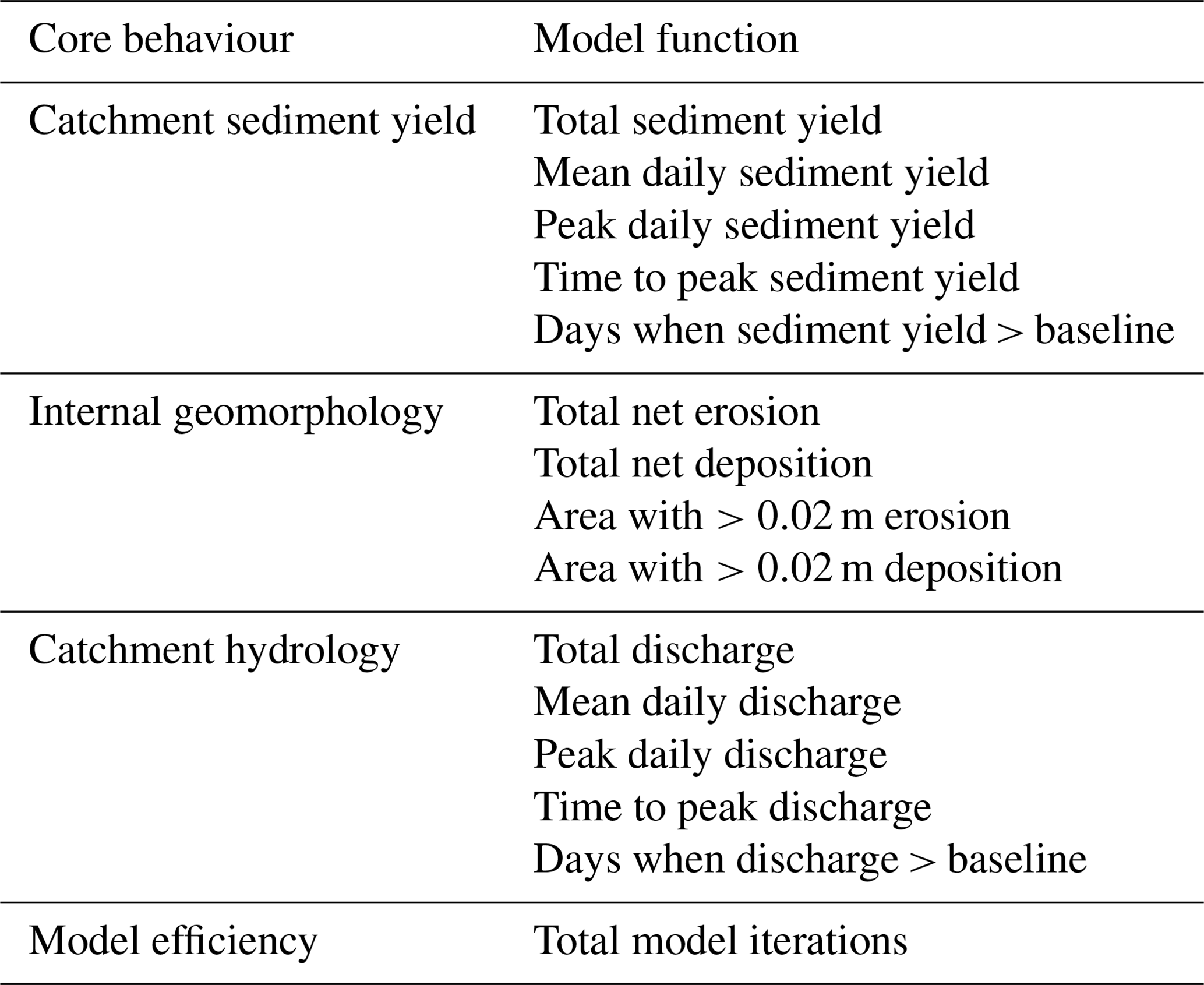
In Skinner et al. (2018), a model function approach to evaluating MM was developed and tested using the CAESAR-Lisflood model. The main purpose of the model function approach was to mitigate for the fact that there is almost always a lack of suitable observation data to use in evaluating the performance of LEMs via an objective function approach (an objective function being the error score between modelled and observed data). Instead, Skinner et al. (2018) proposed a series of metrics that would assess key behaviours in the model relating to its outputs and assess the MM against changes in the model's behaviour. Here, we use the same 15 model functions as Skinner et al. (2018) and these are shown in Table 2. To summarise the large amount of information produced, the ME of each parameter and model function combination was normalised based on the proportion of the ME for highest ranking parameter for that model function – therefore, the highest ranked parameter for each model function always scored 1. The scores for each parameter were aggregated across all model functions based on the mean of the scores. The model functions were further sub-divided into core behaviour groups (Table 2) and the scores aggregated again for each core behaviour. The same was also done, separately, for the standard deviations of each parameter and model function.

The same set of repeats and parameter changes were used for each grid cell size to allow direct comparison. Finally, using the full set of results across all of the grid cell sizes, a further analysis was performed with grid cell size as an additional parameter to assess its relative influence on the model compared to the other seven parameters. This was done by using five steps (4, 8, 12, 16, and 20 m resolution) and randomly selecting the starting grid cell size for each repeat, the position in the sequence it is changed to, and the change in steps.

Each individual test within the repeats consisted of 30 years of simulations using the same input rainfall. The rainfall was produced by using a 23-year observation record from a single rain gauge at Jabiru Airport, with the first 7 years repeated for the full 30-year input. This was applied as a lumped input at a 1 h time step.

2.4 Stream network analysis

To examine how stream network metrics changed with DEM resolution, the Hydrology tools in ArcMap 10.4.1 were used to extract stream networks and stream orders for each resolution with the Strahler (1957) and Shreve (1966) methods. Both methods are top-down approaches to stream ordering in that they start from the source and increase in value towards the outlet. The Strahler method (Strahler, 1957) calculates the depth of the drainage network – a second-order stream begins only where two or more first-order streams meet, and a third-order stream only where two or more second-order streams meet, and so on. As such, the maximum stream order number does not provide information on the number of individual streams within the network. The Shreve method (Shreve, 1966) assigns stream values cumulatively, so where two streams with a value of 1 meet, the downstream becomes 2, and unlike the Strahler method, lower-order tributaries are included in the ordering, so where a stream with a value of 1 joins with a stream with a value of 2, the downstream section is assigned a value of 3. Therefore, the stream number at the outlet provides information on the number of streams in the system. In ArcMap, a stream identification threshold (in effect delineating first-order streams) was set at 1000 m², rounded up to the nearest whole pixels. The total number of first-order streams calculated by the Strahler method was estimated by converting the raster output to a polyline and selecting only first-order streams. With the exception of the 2 m resolution, the analysis was performed on the post-test DEM for Test 1 of each resolution test to allow a drainage network to be established on spin-up into the DEM surface – this negated the need to pit-fill the DEM before the network analysis.

3 Results

3.1 Influence of grid cell size on model outputs (model functions)

The ME for each of the 15 model functions were calculated for each of the grid cell sizes and the patterns observed for each model function are summarised in Table 3. The box and whisker plots of Fig. 2 highlight these patterns for four of the model functions (plots for all of the model functions can be viewed in Appendix B). Figure 2 shows that the mean total erosion and sediment yield outputs by the model remain similar for grid resolutions up to 24–30 m, although the spread of values across the 80 tests vary more with larger grid cells. However, the peak daily sediment yields increase with larger grid cells, whereas there is a decrease in the number of days where sediment yield is over the baseline. This indicates that with larger grid cells, there are less events that produce erosion and sediment outputs offset by an increase in erosion and sediment outputs during larger events.

Table 3 Visual interpretation of influence of grid resolution on the 15 model functions.

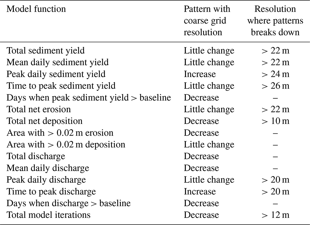
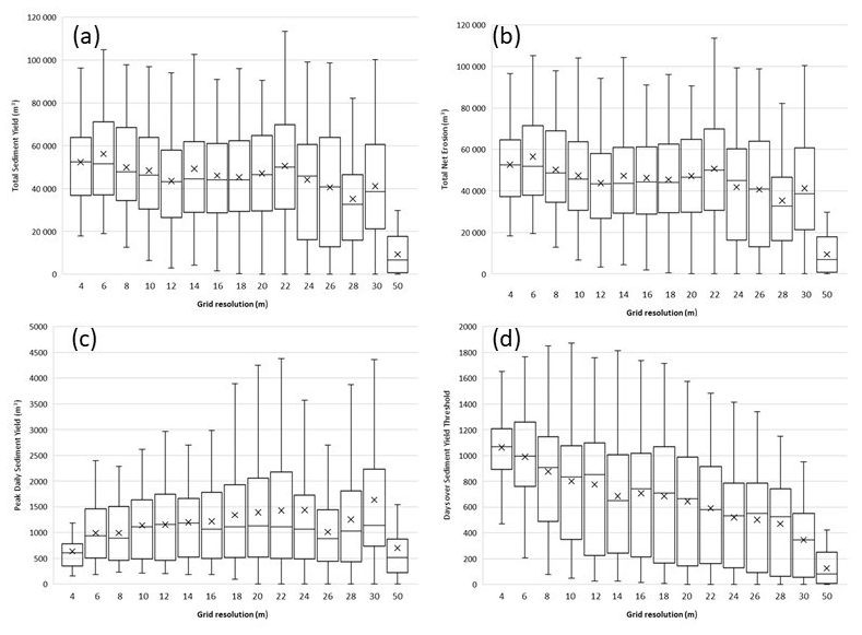
Figure 2 Box and whisker plots showing the mean and spread of model outputs at each grid resolution, for (a) total sediment yield, (b) total net erosion, (c) peak daily sediment yield, and (d) days over sediment yield threshold.

The box and whisker plots in Fig. 2 aggregate the results of 80 tests and could conceal a range of varying model behaviours when using the same parameter set across the different grid cell sizes. To check this, five parameter sets, or tests (numbered as the order they appear in the MM), were randomly selected and plotted in Fig. 3. This shows that the individual tests follow the overall trends displayed in Fig. 2.

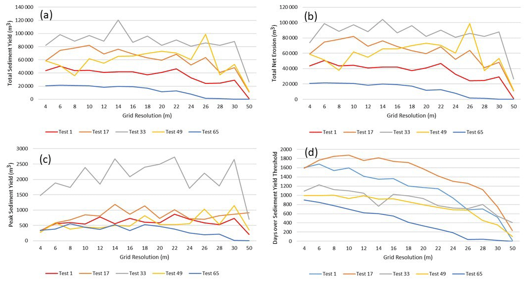
Figure 3 Output values for five randomly selected test numbers at each grid resolution for (a) total sediment yield, (b) total net erosion, (c) peak sediment yield, and (d) days over sediment yield threshold.

3.2 Influence of grid cell size on model behaviour (summary of MM)

The mean aggregated ME scores, measuring the overall relative influence of each parameter across all of the model functions, are shown in Fig. 4. Although there is variation between the grid cell sizes, the relative influence of each parameter remains fairly consistent across DEM resolution. The clear exception here is the Sediment Transport Law: while it remains the most influential parameter for the majority of resolutions, its relative influence decreases as the grid coarsens, until for the coarsest of grids, the TOPMODEL M replaces it as most influential (at 28 and 50 m). It appears that it is an increase in influence of the TOPMODEL M that drives the decrease below 26 m, beyond which all the other parameters increase in influence as the Sediment Transport Law further decreases.

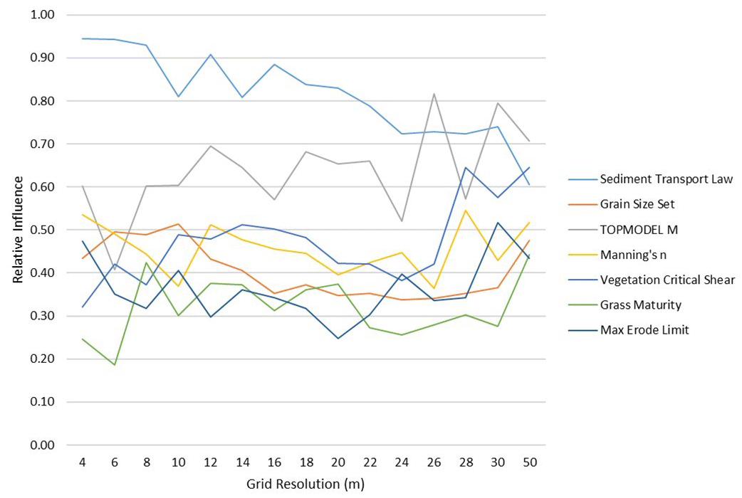
Figure 4 Mean ME scores aggregated for all model functions for each parameter and each grid cell size.

3.3 Stream network analysis

The numbers of stream orders calculated is shown in Fig. 5. The maximum number of stream orders calculated by the Strahler method remained consistent throughout, dipping to three orders at 28 m resolution, and three again at 50 m. The Shreve and Strahler first-order counts steadily decreased as grid cells become larger. This shows that the depth of the drainage network does not reduce until the largest grid cells are used. However, the detail within the network is being lost with less first-order Strahler streams, and lower Shreve numbers, with larger grid cells. The disparity between the Shreve number and the number of first-order Strahler streams is due to disconnection of part of the drainage channel to the main network; therefore, these streams are not contributing to the Shreve number. This disconnection was not consistent through the resolutions, with some coarser resolutions displaying a better connected network than others.

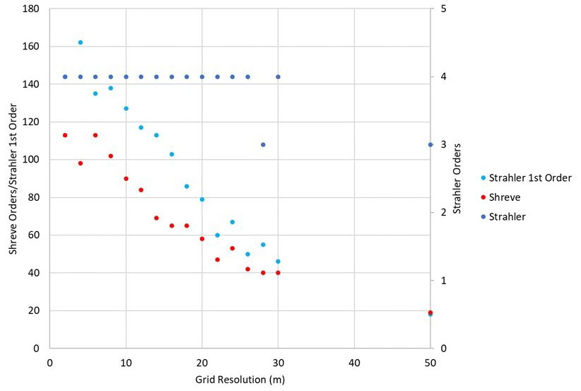
Figure 5 The maximum number of stream orders calculated at each grid resolution using both the Strahler and Shreve methods. The total number of first-order stream cells calculated by the Strahler method is also shown.

3.4 Model performance

Figure 6 shows the changes in the number of iterations required by the model with each grid cell size. The iterations represent the number of calculations required by a test and is a useful proxy for model efficiency that is independent of the specification and performance of individual machines. There is a visible rapid drop off in the number of iterations required between 4 and 12 m resolutions, yet little change with increasing coarseness beyond 12 m, suggesting that there are only marginal computational efficiency gains to be made using DEM resolutions coarser than 12 m (the spread of the total number does decrease beyond 12 m still).

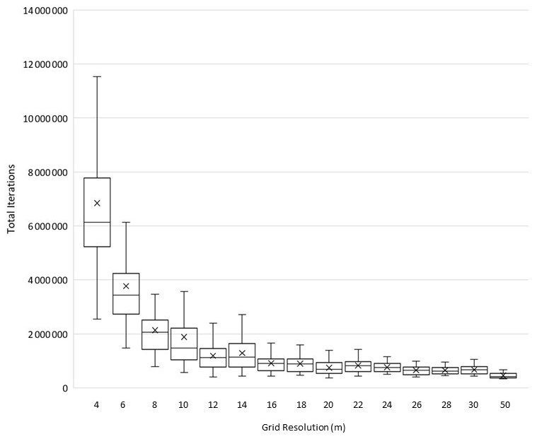
Figure 6 Box–Whisker plots showing the spread of total number of model iterations required at each grid resolution.

3.5 Relative influence of grid cell size

The results from the MM tests for each grid cell size were further used to simulate an MM run where the DEM grid resolution could be considered a parameter itself. Figure 7 summarises the results and reveals the relative importance of grid cell sizes when compared to the key parameters in the model. Overall, it has a similar level of influence over all core behaviours as the Sediment Transport Law (i) and the TOPMODEL M. Broken down, this is skewed by the Catchment Hydrology (iii) and Model Efficiency (v) core behaviours where it is the most influential parameter, whilst it has relatively low relative influence on the Catchment Sediment (ii) and Internal Geomorphology (iv) behaviours.

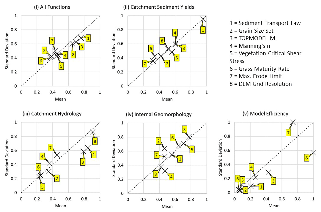
Figure 7 Mean and standard deviation of relative MEs for the seven parameters and DEM grid resolution for all model functions aggregated by core behaviours (see Table 2).

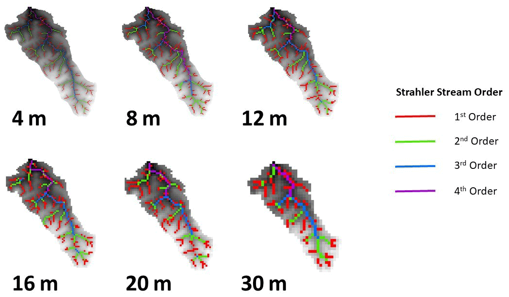
Figure 8 Illustration of the loss of granularity in the representation of the stream network with increasingly large grid cell sizes.

4 Discussion

4.1 Model robustness to grid resolution

Certain aspects of CAESAR-Lisflood's performance are relatively robust to changes in grid cell size. However, this behaviour can conceal important differences. As shown in Table 3 and Figs. 2 and 3, important factors including total sediment yield and total net erosion display little change until grid cell sizes > 22 m. However, whilst these output metrics remain relatively constant, related factors, i.e. peak daily sediment yield increase, and days when peak sediment yield is > threshold decrease. Despite long-term sediment yields being similar, this demonstrates a change in model behaviour, where with larger grid cells, the sediment delivered from the catchment is doing so in fewer yet larger bursts. This can be explained by a loss of the granularity of the drainage network as grid cell size increases, as shown in Fig. 8. In particular, first-order streams are lost with larger grid cells (see Fig. 5). With smaller grid cells, there is a more detailed channel network, so when summed across the whole basin, the process of channels geomorphically “switching on and off” is smoother. With larger grid cells, there are less channels, meaning the switching on and off response is more step like and thus more spiky. This also illustrates one of the weaknesses and difficulties of using a lumped parameter such as basin sediment yield to describe both model performance and basin geomorphology. There was also a decrease in total net deposition with larger grid cells, consistent with the findings of Schoorl et al. (2000), who found that using larger grid cells makes the conditions needed for sedimentation less likely to occur. We did not see any of the larger grid-dependent erosion fluctuations demonstrated by Nicholas (2005) with their braided river model. This can be explained by CAESAR-Lisflood using the flow velocity derived from water surface slope to calculate bed shear stress and thus sediment transport rather than bed slope. In other LEMs based on bed slope, this sensitivity may therefore remain.

4.2 Model behaviour with grid resolution

The behaviours of the model are captured by the relative influence of parameters on the model functions and core behaviours, with changes in the relative influence being taken as a change in behaviour. The relative influence of the seven parameter tests on the core behaviours when using different grid cell sizes is summarised in Fig. 4 and suggests a similar story to the changes in factors that would indicate model robustness. Although there is some noise, the relative importance of the different parameters remains relatively unchanged below the coarsest resolutions > 22 m. However, there is also a general trend of waning influence of the choice of Sediment Transport Law that appears to begin at 10 m resolution and continues throughout. This indicates that the coarsening of the grid resolution is resulting in some key behavioural shifts in the simulations that are most likely related to the loss of detail in the drainage network discussed in Sect. 4.1.

Relative to the seven parameters used in the MM tests, grid cell size showed a mixed degree of influence on the model behaviours (see Fig. 7). Grid cell size had the greatest influence on the model efficiency, which also had a relatively low standard deviation ME, suggesting that this was non-linear and other parameter values did not affect this. This is exactly as would be expected since halving the grid cell size increases cell number by 4, which also increases the number of computations per iteration required by the same factor. Grid cell size had the greatest influence over the catchment hydrology behaviours, which is consistent with the loss of detail in the drainage network discussed in Sect. 4.1 and also the findings of Savage et al. (2016) that grid resolution influences the sensitivity of hydraulic models to parameter values. It had relatively less influence over the catchment sediment and internal geomorphology behaviours but still influential enough to require consideration. Overall, grid resolution was shown to be the third most influential parameter, to a similar degree as the Sediment Transport Law and TOPMODEL M.

4.3 Implications and limitations

This work has only simulated the influence of grid cell size on a single LEM and on a single, relatively small, catchment. The role of the loss of detail in the drainage network with larger grid cells is a physical effect applicable across all models using a regular grid of elevation and to any catchment, regardless of size or situation. However, the relative impact will change with different size basins – at different resolutions – and quite possibly when experiencing a different range or magnitude of driving events. Therefore, the generic finding of our study – that the degradation of a model DEM (larger grid cells) conceals topographic details that may be important to model outcomes – is important. However, the actual impact on individual studies will be specific to the catchment modelled and the resolution chosen.

This study has further highlighted the need for operators to better understand the sensitivities of their models to both internal and external factors before embarking on landscape evolution studies. Here, we have demonstrated that DEM grid resolution is a controlling external factor of the behaviours simulated in the system, with larger grid cells resulting in fewer yet more extreme erosion producing events, which although overall produces similar total sediment yields, does so over a smaller contributing area. Grid cell size was also shown to be the third most influential parameter out of those tested. This suggests that when making model choices, it is important that operators should aim to use the finest resolution available to them and that model efficiency will allow. Where model efficiency is a concern, a compromise can be made by selecting a resolution where coarsening further results in lower levels of benefits – in this study, that would appear to be around 12 m (Fig. 6), close to the default 10 m used for the same catchment in Skinner et al. (2018). Importantly, this choice is catchment-specific.

The use of MM to assess the model's sensitivity to external factors (e.g. grid cell size) relative to the sensitivity to internal parameters presents opportunities and a powerful tool. This allows for a more comprehensive consideration of the sensitivity of the model to choices of the modeller and enable them to evaluate which areas to focus on improving, for example, the tests here tell the modeller that work to increase the resolution and detail of the DEM grid would yield greater benefits than work to reduce the uncertainty in the grain size parameters. Performing this type of analysis to inform model choices will increase the robustness and confidence in model outputs, crucial if LEMs are going to be used operationally and for decision-making. Additionally, the same methods can be applied to other modelling fields, including hydrological and hydraulic modelling.

Whilst this study has highlighted the influence that grid cell size can have on model behaviour and outputs, it is also limited by the narrow set of conditions tested. We have only considered a single LEM and only a single small catchment with its own unique set of conditions. Therefore, whilst many of our findings can reasonably be ported to different models with similar parameterisation and operation, we acknowledge that the findings are not generic. Equally, whilst we believe that many of our findings are directly relevant to other applications of CAESAR-Lisflood to different catchments, Tin Camp Creek has few depositional zones (e.g. floodplains or alluvial fans), so the majority of eroded sediments leave the catchment entirely. We have deliberately used a short timescale of simulation, just 30 years, that is short by the standards of LEMs but analogous to operational uses of the models to aid decision-making. Therefore, the applicability of the detailed results of this study to other models, catchments, and timescales is unknown.

However, we suggest that several findings will be relevant to many LEM-based studies. Namely, (1) using water surface slope instead of bed or cell to cell slope for calculating fluvial erosion is more resilient to different grid cell resolutions; (2) the degradation of the representation of the landscape with increased grid size is most acutely felt in first-order streams; (3) CAESAR-Lisflood is unusual in the LEM community by simulating individual flood events and above we observed that more sediment was being delivered in fewer events with increasing resolution. If or how this effect is found in LEMs using constant or slowly varying representations of climate/rainfall/discharge remains an important and open question for long-term LEM studies; (4) the sensitivities of models to grid cell resolutions should be understood as part of any study using LEMs. This is particularly pertinent when they are being used operationally.

5 Conclusions

This research has explored the influence DEM grid cell size has on the water and sediment outputs of a LEM (CAESAR-Lisflood) using the Morris method sensitivity. We found that simulated basin sediment yields and hydrological outputs totalled over the model duration were largely unchanged as grid cells sizes increased, up to a point where the grid cell size started to degrade the extent and shape of the drainage network. It is likely that the impact of this network degradation will be dependent on the size of the basin, with the results being lessened on larger basins for the same grid cell size.

However, when the model results are analysed over event-scale timescales, it became clear that the lumped output grid-scale independence masked important changes with resolution. As grid cell sizes increased, the similar sediment yields were produced by fewer, larger events. It is important, therefore, to note this sensitivity in the model's application or risk a “right results for the wrong reasons” set of outputs.

These findings are important because the resolution of the DEM used in LEM studies is often an arbitrary choice, often driven by the need to balance including as much detail as is available with model efficiency. The approach presented in this paper demonstrates the feasibility of using a screening sensitivity analysis to identify key influences on model behaviour, for grid cell size, and parameter choices, which will help modellers identify the optimal grid cell sizes for their study.

Appendix A: Description of parameters

Table A1 Description of CAESAR-Lisflood parameters considered as part of the Morris method test.

Appendix B: Box and whisker plots

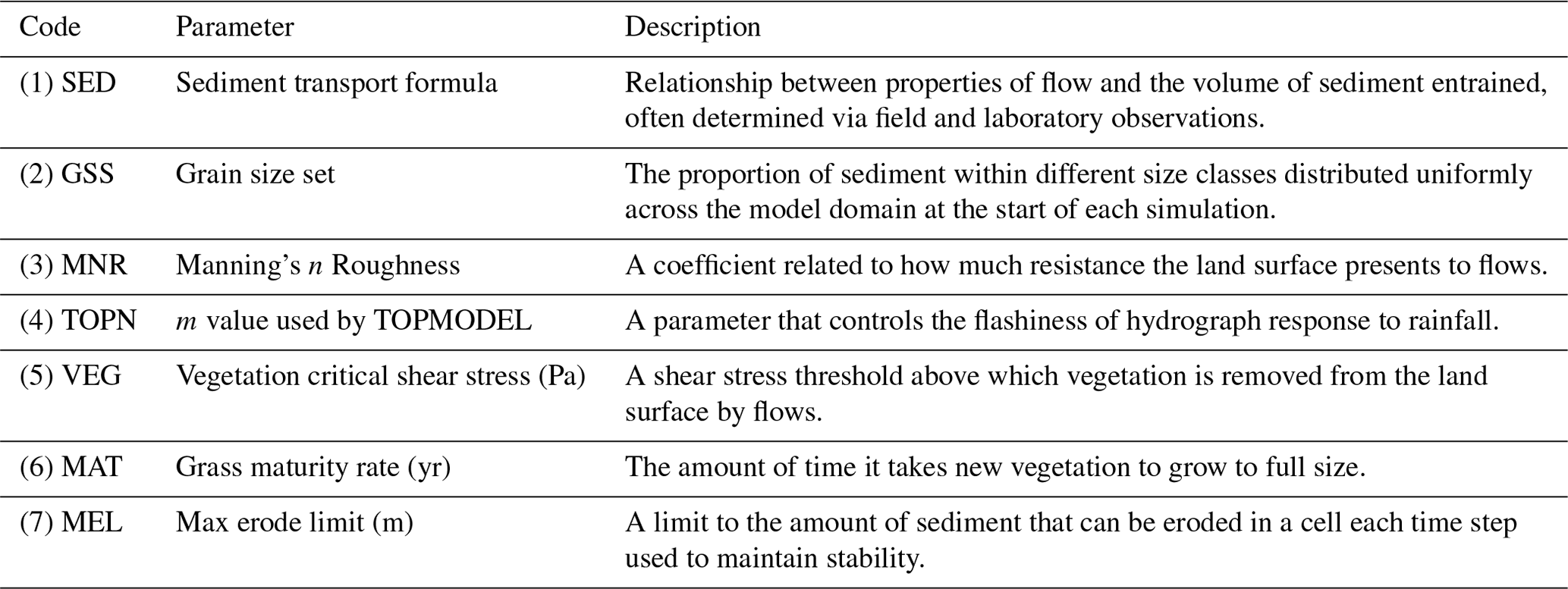
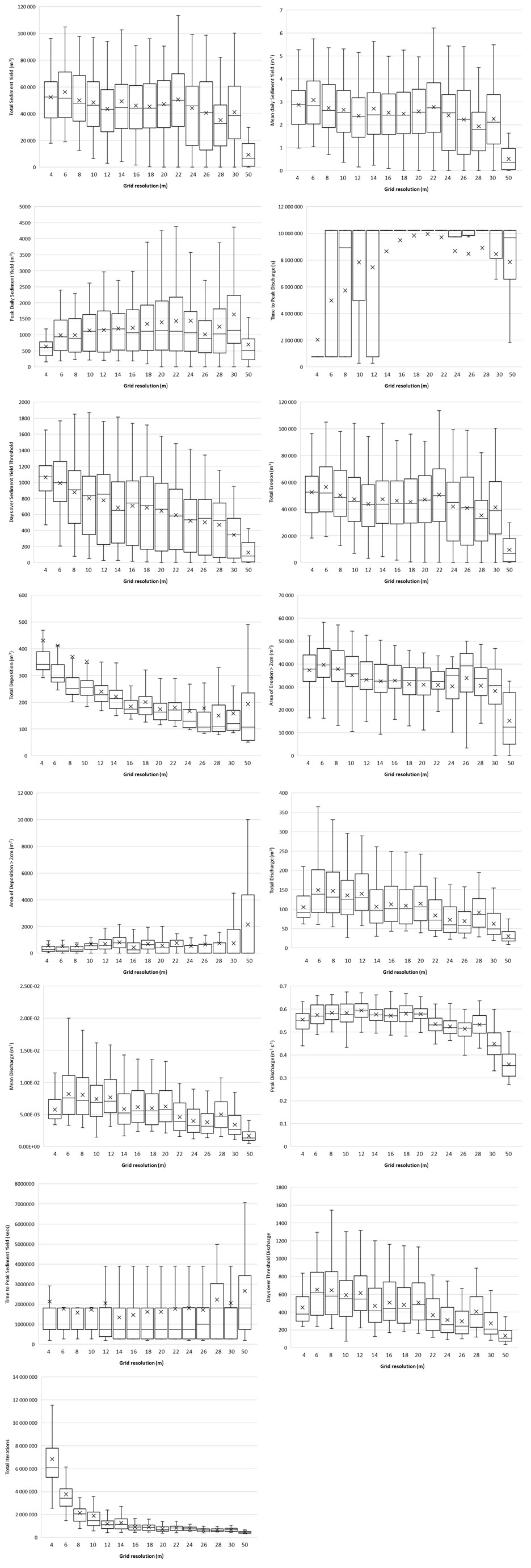
Figure B1 Box and whisker plots showing the spread of model outputs and the means at each grid resolution.