Stream laws in analog tectonic-landscape models

The interplay between tectonics and surface processes defines the evolution of mountain belts. However, correlating these processes through the evolution of natural orogens represents a scientific challenge. Analog models can be used for analyzing and interpreting the effect of such interaction. To fulfill this purpose it is necessary to understand how the imposed boundary conditions affect analog models' evolution in time and space. We use nine analog models characterized by different combinations of imposed regional slope and rainfall rates to investigate how surface processes respond to the presence of tectonically built topography (imposed slope) under different climatic conditions (rainfall rate). We show how the combination of these parameters controls the development of drainage networks and erosional processes. We quantify the morphological differences between experimental landscapes in terms of a proposed $S_{\mathrm{e}}/R$ ratio, accounting for both observables and boundary conditions. We find few differences between analog models and natural prototypes in terms of parametrization of the detachment-limited stream power law. We observe a threshold in the development of channelization, modulated by a tradeoff between applied boundary conditions.

1 Introduction

Accurately interpreting the continuous interaction between tectonics and surface processes in mountain belts is one of the main challenges that geologists have faced in the last century. Many limitations exist due to the different depths and spatial and temporal scale at which crustal and mantle processes impact the surface. Thus, it is difficult to univocally interpret how different factors interact to build the present-day landscape. Analog models allow for a useful direct control of the evolution of the studied physical process (e.g., Reber et al., 2020), overcoming many of these limitations. Tectonics, erosion, and sedimentation play an integrated role in the evolution of mountain belts with complex and poorly constrained feedbacks. During the last decades modelers analyzed these feedbacks, from the rejuvenation of streams (e.g., Schumm and Parker, 1973; Schumm and Rea, 1995) to the more complex evolution of whole orogenic systems (e.g., Bonnet, 2009; Graveleau and Dominguez, 2008; Guerit et al., 2016; Lague et al., 2003; Tejedor et al., 2017; Viaplana-Muzas et al., 2019; Reitano et al., 2022b). However, all the previous analog modeling efforts are based on the robustness of the characterization of material used in the experiments (e.g., Graveleau et al., 2011; Reitano et al., 2020) and on the scaling to natural prototypes (e.g., Graveleau et al., 2011; Paola et al., 2009). While the mechanical, frictional, and erosional properties have been characterized empirically and analytically by different authors (Bonnet and Crave, 2003; Lague et al., 2003; Graveleau et al., 2011; Reitano et al., 2020), the application of erosion laws to analog systems is still a matter of debate. In particular, a definition of the response of the analog materials to the applied boundary conditions and an understanding of the variables that modify this response are still missing. These characterizations become even more important considering that a perfect scaling between natural- and experimental-flow laws is currently missing, limiting the reach of analog studies to insights derived from qualitative process similarity (Paola et al., 2009).

In this work we analyze how different boundary conditions affect the evolution of analog landscapes, in terms of tectonically built topography (imposed regional slope) and climate (rainfall rate). The methodologies implemented here allow us to isolate how these different a priori conditions control features like channelization, morphometrics, and incision rates. We then define the ranges of boundary conditions in which different morphological features develop (e.g., channels or diffusive processes). Finally, we discuss if and how the erosional parametrization implemented in nature (stream power law) applies to analog models. Analog models run in this study are representative of the slow-tectonic regions (e.g., very low uplift/erosion rate such as the Anti-Atlas of Morocco; Lanari et al., 2022; Clementucci et al., 2022) or passive margins such as the Western Ghats escarpment in the eastern margin of peninsular India (Mandal et al., 2015; Wang and Willett, 2021) and the southern Australian escarpment (Godard et al., 2019), where the uplift variation in space is negligible.

2 Experimental setup, scaling, and erosional laws

The analog material is a granular, water-saturated mixture made of 40 wt % of silica powder, 40 wt % of glass microbeads, and 20 wt % of PVC powder (Reitano et al., 2020). We fill a $\mathrm{35}\times \mathrm{30}\times \mathrm{5}$ cm³ box with the material and place it on a reclinable table (Fig. S1 in the Supplement). The rainfall system is made of nozzles that provide a dense fog to trigger surface processes. The droplet size in the fog is lower than 100 µm to avoid rain splash erosion (e.g., Graveleau et al., 2012). We apply three different rainfall rates in the models (9, 22, and 70 mm h⁻¹) by controlling the number of implemented nozzles. The homogeneity of rainfall distribution has been tested as described in detail in the Supplement of Reitano et al. (2022b). The angle between the table and the horizontal (i.e., imposed regional slope) is also fixed at three different values, 10, 15, and 20^∘. Both rainfall rate and imposed regional slope are kept constant throughout the experiments. In total, we investigate nine different imposed regional slope–rainfall rate configurations (Table S1 in the Supplement). We use a camera to capture top-view digital images of the experiment evolution and a high-resolution laser scanner to acquire DEMs at defined time steps. The vertical and horizontal resolutions of the laser are 0.07 and 0.05 mm, respectively.

Considering a length scaling factor $L^{*}={\mathrm{10}}^{-\mathrm{5}}/{\mathrm{10}}^{-\mathrm{6}}$ (1 cm = 1–10 km), a gravitation acceleration scaling factor $g^{*}=\mathrm{1}$, and a velocity scaling factor $v^{*}={\mathrm{10}}^{\mathrm{4}}-{\mathrm{10}}^{\mathrm{5}}$ (1 cm h⁻¹ = 0.1–1 cm yr⁻¹), the time scaling factor t^* is computed by (Reitano et al., 2020, 2022b)

$$\begin{array}{}\text{(1)}& t^{*}={\displaystyle \frac{\mathrm{4}{L}^{*}}{v^{*}}},\end{array}$$

such that 1 min in the models corresponds to 5 to 50 kyr in nature.

The change in elevation (dz) over time (dt) of a point on the surface results from the competition between the rock uplift rate U and the erosion or sedimentation rate E:

$$\begin{array}{}\text{(2)}& {\displaystyle \frac{\mathrm{d}z}{\mathrm{d}t}}=U-E.\end{array}$$

For fluvial networks that show exposed bedrock at the base, the erosion rate is typically expressed as a function of a “detachment-limited stream power law” (e.g., Goren et al., 2014b, a; Howard, 1994; Howard and Kerby, 1983; Tucker and Whipple, 2002):

$$\begin{array}{}\text{(3)}& E=\mathit{\kappa }{Q}^m{S}^n,\end{array}$$

where κ is the bedrock erodibility; Q is the channel discharge; S is the channel slope; and m and n are exponents accounting for channel geometry, basin hydrology, and erosion processes. Since Q is a function of drainage area, A, and the rainfall rate, P (Q=AP), Eq. (3) can be rewritten as

$$\begin{array}{}\text{(4)}& E=K{A}^m{S}^n,\end{array}$$

where K=κP^m is controlled by bedrock lithology, incision process, and climate (here rainfall rate). In a stream channel, Flint's law describes the power relationship between channel slope S and drainage area A (Flint, 1974):

$$\begin{array}{}\text{(5)}& S=k_{\mathrm{s}}{A}^{-\mathit{\theta }},\end{array}$$

where k_s and θ are the channel steepness and the concavity indexes, respectively (e.g., Wobus et al., 2006a; Kirby and Whipple, 2012; Hack, 1957, 1960). Merging Eqs. (4) and (5) and considering that $\mathit{\theta }=m/n$, we can express the result in a logarithmic form:

$$\begin{array}{}\text{(6)}& {\log }_{\mathrm{10}}E=n{\log }_{\mathrm{10}}{k}_{\mathrm{s}}+{\log }_{\mathrm{10}}K.\end{array}$$

Equation (6) is thus the equation of a line ($y=mx+q$), where n and log ₁₀K are the slope and the intercept, respectively.

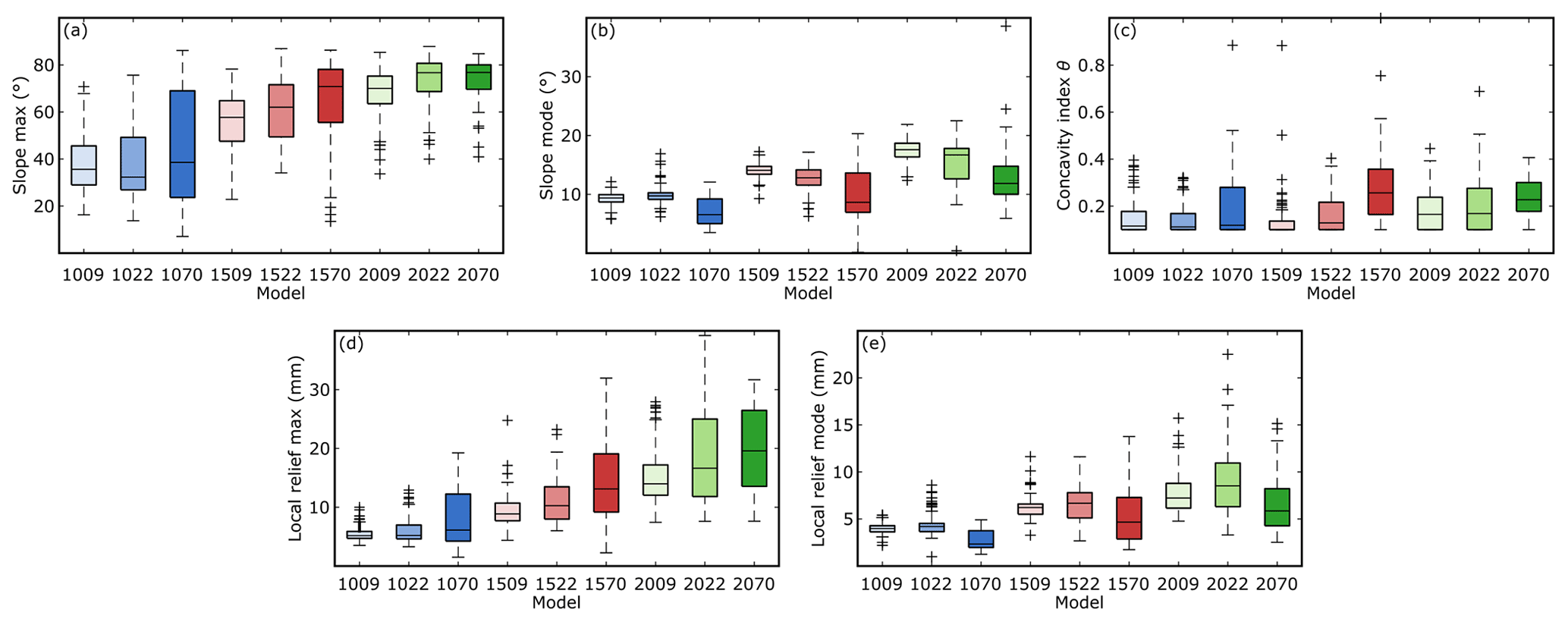
Figure 1 Geomorphological and channel metrics of the performed experiments. The solid black lines indicate the median, while the bottom and top edges of the colored boxes indicate the 25th and 75th percentiles, respectively. The black whiskers outside the boxes cover the data points at the < 25th and > 75th percentiles that are not considered outliers, here indicated by black crosses. The color saturation in the boxes is related to the applied rainfall rate (less saturated, lower rainfall rate). The blue, red, and green boxes refer to models at imposed slopes of 10, 15, and 20^∘, respectively.

From the DEMs we compute (i) topographic metrics such as basin slope (max and mode) and local relief (max and mode); (ii) channel metrics (k_s and θ) and channel profiles (concavity index, θ, as well as steepness index, k_s, has been extracted by power law regression between local slope and area – Flint's law); and (iii) eroded volumes, incision rate, and erosion maps. We describe the methodologies used for extracting the eroded volumes and incision rates in the Supplement. The abovementioned analyses are performed using the TopoToolbox package (Schwanghart and Scherler, 2014).

3 Results

Table S1 shows a list of the performed experiments, where the first and last two digits of the models' name represent the imposed regional slope and the imposed rainfall rate, respectively (e.g., mod1522: imposed regional slope of 15^∘ and rainfall rate of 22 mm h⁻¹). These model runs are interpreted highlighting the effect of boundary conditions on the evolution of geomorphic models. Results refer to 10 time steps that highlight key stages in the evolution of each model (Supplement) or to the entire experimental run (300 min). For every model at every time step, we defined and extracted all the basins forming and developing into the landscape, together with the main river trunk (max length) for every basin. For these basins we calculated the maximum surface slope (SS_max), the surface slope mode (SS_mode), the maximum local relief (LR_max), the local relief mode (LR_mode), and the concavity index (the last one from the main river in the basin). Increasing the imposed regional slope (from mod1009 to mod2070), the SS_max increases systematically from 30 to 80^∘ (between the 25th and 75th percentile; Fig. 1a). The general increase in SS_max between models 1009, 1509, and 2009 (and the same for different rainfall rates) reflects the imposed slope increase since values are not normalized for the imposed slope. Still, increasing the imposed rainfall rate also results in an increase in SS_max. Conversely, SS_mode decreases for models with the same regional slope but increasing rainfall rates (e.g., mod1509, mod1522, mod1570), except for mod1009 and mod1022 (Fig. 1b), whereas the mode increases for models with the same rainfall rate but different imposed regional slopes (e.g., mod1009, mod1509, mod2009). Models with a rainfall rate of 70 mm h⁻¹ show the lowest values in SS_mode yet the broadest range of values (between 5 and 15^∘ from mod1070 to mod2070). The decreasing trend in the SS_mode is also observed in the morphological expression of the model's surface (Fig. 2a). The models with a rainfall rate up to 22 mm h⁻¹ show clear channelization during the final stage of the evolution, while models with rainfall rates equal to 70 mm h⁻¹ shown little to no channelization in the final stage. Only mod2070 develops well-defined channels (branching, narrow channels, incision concentrated in valleys and channels).

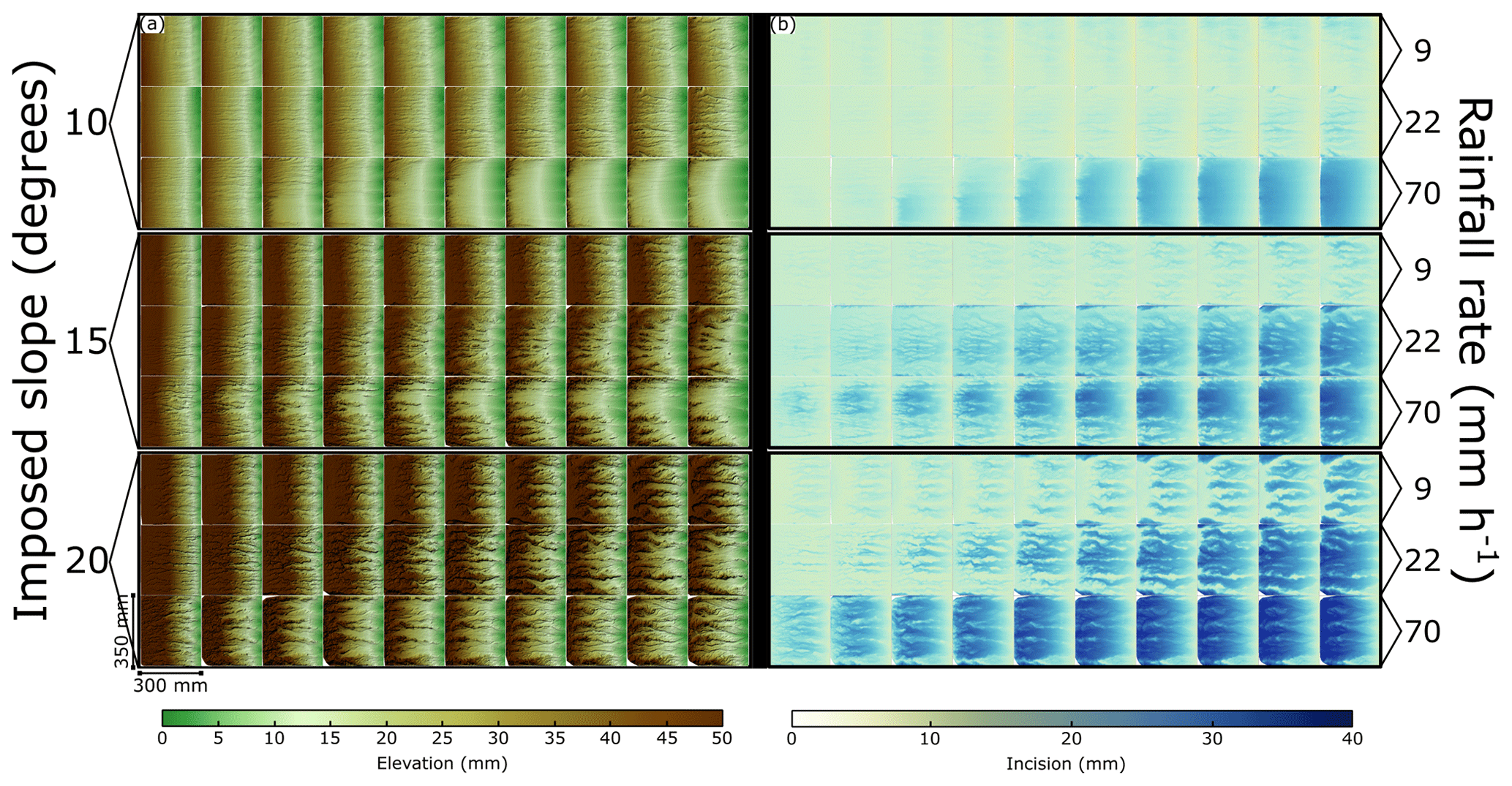
Figure 2 (a) DEMs and (b) erosion DEMs of the performed experiments. The erosion DEMs are obtained by computing the difference in elevation (Δz) of the same cell at consecutive times.

The concavity index ranges from 0.1 to 0.4 (between the 25th and 75th percentile; Fig. 1c). Models with the highest rainfall rate typically show the highest concavity values, correspondingly with the highest variability (mod1070, mod1570, mod2070; Fig. 1c). The local relief was extracted using a moving window with a radius of 10 mm. The maximum local relief LR_max and local relief mode LR_mode show a similar pattern with respect to the surface slope (Fig. 1d and e). LR_max increases from mod1009 to mod2070, while the LR_mode decreases for models with rainfall rates equal 70 mm h⁻¹ with respect to models with the same imposed regional slope but different rainfall rates. The same information can be deduced by visual inspection of DEMs (Fig. 2a).

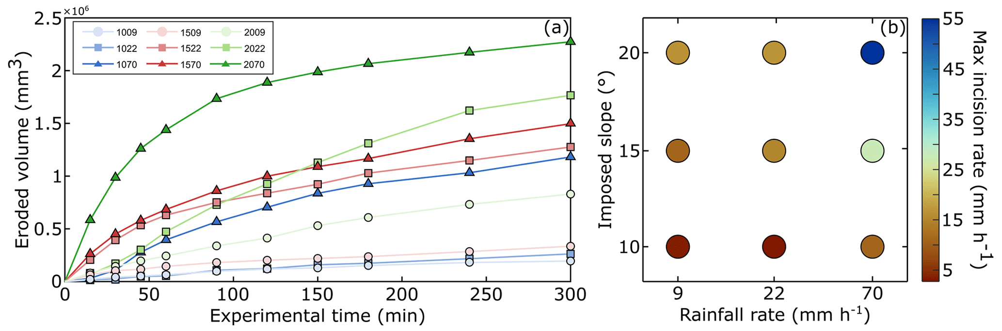
Figure 3 (a) Amount of eroded material for the performed experiments (the color coding follows Fig. 1). (b) Maximum incision rate as a function of the imposed boundary conditions.

The amount of eroded material ranges from 0.2×10⁶ (mod1009) to 2.3×10⁶ mm³ (mod2070) in the last stage of the experiments' evolution (Fig. 3a). Both increased rainfall rate (e.g., mod1009, mod1022, mod1070) and increased imposed regional slope (e.g., mod1022, mod1522, mod2022) result in higher amounts of eroded material. All models show an initial phase where the material flux is highest with a later phase of decline (Reitano et al., 2020), tending toward stability. For example, in mod2070, 60 min of experimental time is enough to erode 1.4×10⁶ mm³ of material, while in the next 240 min only an additional 0.9×10⁶ mm³ of material is eroded. This different behavior is most apparent in models with high rainfall rates (≥22 mm h⁻¹) and slopes (≥15^∘). The maximum incision rate increases with the imposed regional slope and rainfall rate (Fig. 3b), from <5 mm h⁻¹ (mod1009) to ca. 55 mm h⁻¹ (mod2070).

We extract values for E and k_s of four main channels for each time step and for every model (40 channels per model, total = 360). From these values, we obtain n and K by linear regression (Sect. 2). Despite the low R² values (0.01–0.28; Fig. 4), n ranges between −0.18 and 0.14 with K values between 0.77 and 23.51 mm^1−2m h⁻¹. Values of K increase as a function of the slope and rainfall rate, while n does not show a clear trend. On the right-hand side of Fig. 4, we plot data for models with the same imposed regional slope but different rainfall rates. Models with the same regional slope show a gradually increasing k_s and incision rate in response to increased rainfall rates (Fig. 4b). Interestingly, estimates of K gradually increase in models with imposed regional slopes of 10 to 20^∘ (Fig. 4b).

4 Discussion

4.1 Type of erosion as a function of boundary conditions

Our analog models are controlled exclusively by imposed regional slope and rainfall rate, as no other boundary conditions are applied (e.g., vertical uplift or horizontal advection of material). Higher rainfall rates (70 mm h⁻¹ in this work) tend to inhibit the development of a channelized and branching channel network in favor of more diffusive and mass wasting processes. This trend can be deduced by analyzing the DEMs of mod1070 and mod1570 (Fig. 2a) or simply by noting the diffuse nature of erosion under high-rainfall-rate conditions (Fig. 2b). In this case, the water cannot channelize into discrete features since the amount of water is higher than the channelization capacity of the model, mainly controlled by the imposed slope. Indeed, more diffusive processes develop over a greater area, accounting for the lack of channelization. Even if these models are mainly controlled by diffusive processes, mod2070 exhibits more channelization than mod1070 and mod1570, but, similarly, mod1570 shows slightly more channelization than mod1070. These observations suggest that, in terms of channelization, the higher the slope, the more effectively a system responds to high rainfall rates. Considering the relationship between channelization and boundary conditions, the results of our experiments suggest that low imposed regional slope (mod1009, mod1022) or low rainfall rate with an average imposed regional slope (mod1509) results in a channelization characterized by low incision values (<25–30 mm in the final stage). It thus appears that a threshold exists in rainfall rate for the development of channelized networks, modulated by the slope over which erosion acts. For example, a rate of 70 mm h⁻¹ (mod1070 and mod1570) is too high for a proper channel network to develop, while a higher imposed regional slope (mod2070) provides sufficient potential energy for the system to channelize (e.g., Burbank and Anderson, 2011). Thus, the tradeoff between imposed regional slope and rainfall rate controls the channelization. For higher rainfall rate (mod1070 and mod1570), a sheetlike runoff lowers the model slope homogeneously (Fig. 1b). Furthermore, both the SS_mode and the LR_mode drop with respect to the models with the same imposed regional slope but a lower rainfall rate. From these observations, we argue that at a high rainfall rate, channelization is subordinate to diffusive processes (controlled by ridge stability) in the final stages of model evolution. In landscapes where incision is a function of the detachment of particles from the riverbed, the erosion rate is proportional to the shear stress (e.g., Whipple and Tucker, 1999; Yanites et al., 2010). Higher rainfall rates (i.e., higher water discharge) increase the effective shear stress on riverbeds (Thoman and Niezgoda, 2008). Since water discharge also increases the channel width (e.g., Shibata and Ito, 2014; Wobus et al., 2006b), for high water discharges (i.e., rainfall rate) the shear stress can be distributed over time over wide and flat surfaces instead of concentrating in valleys (Lamb et al., 2015, and references therein). At high rainfall rates our models show incipient channelization in the initial stages (Fig. 2b). Channelization is lost in favor of more diffusive processes during late stages of model evolution. High rainfall rates (i.e., high water discharge) lead to a higher sediment supply that can widen channels (Finnegan et al., 2007; Johnson and Whipple, 2010), eventually erasing their morphological expression. Finally, we must address the erosional threshold defined in the works of Lague et al. (2003) and Graveleau et al. (2011). This threshold must be overcome before significant erosion and transport occurs and specifically apply to models with low imposed regional slopes, which may thus lead to even less channelization.

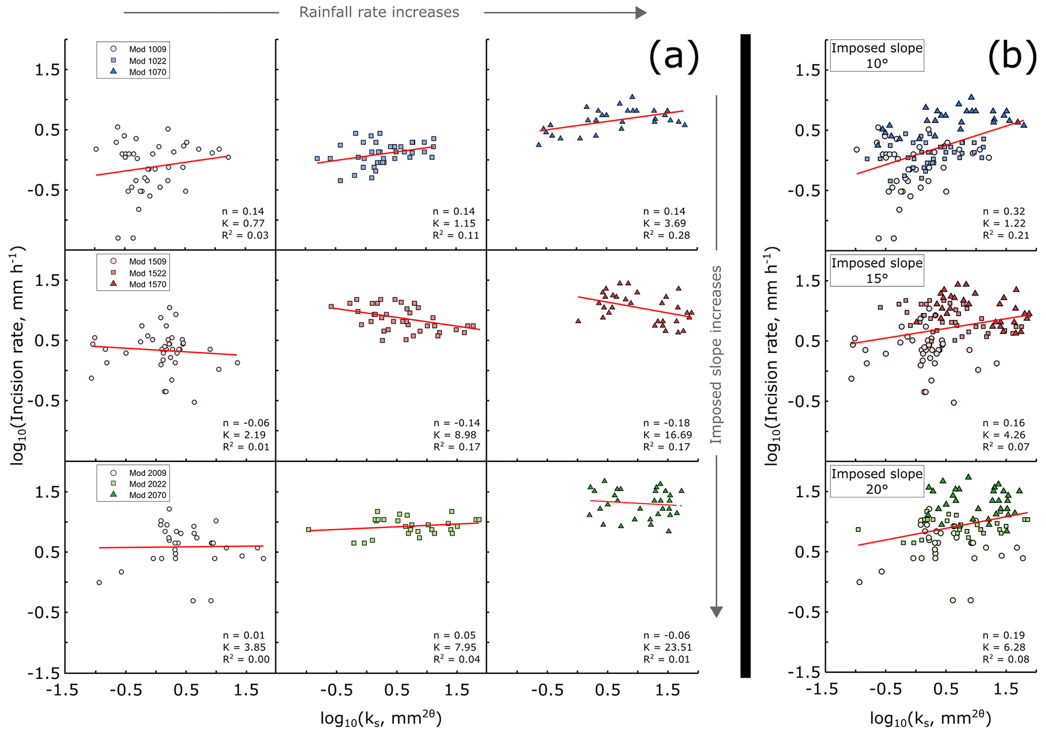
Figure 4 (a) Logarithm of the incision rate over the logarithm of the steepness index k_s for all the models. The imposed regional slope increases from top to bottom. Rainfall rate increases from left to right. Every plot shows 4 channels at every time step (40 channels in total; colored dots). The linear regression is shown by the red line. Values related to the linear regression (n and K) are shown in the bottom right corner of every plot, together with R² (units for K are mm^1−2m h⁻¹). (b) Same data as (a), but plotted for every slope without differentiating for rainfall rate.

Interestingly, effective channelization does not affect the volume of eroded material, which increases with the imposed regional slope and rainfall rate (e.g., the erosion flux is higher in mod1570 than mod1522 and mod1070).

We plotted the volume of eroded material at every time step normalized by the imposed slope and the rainfall rate (V_norm; Fig. 5a). We observe a transient behavior for all the models during the first 100–150 min, indicating the adjustment of the model to the applied boundary conditions. After this transient phase, a steady phase develops, where the system tends toward equilibrium in terms of eroded material. Ideally, due to how V_norm is computed, all lines should collapse into one. This is not the case because analog models are intrinsically stochastic; thus unconstrained variability between the models causes deviation in the calculation of V_norm.

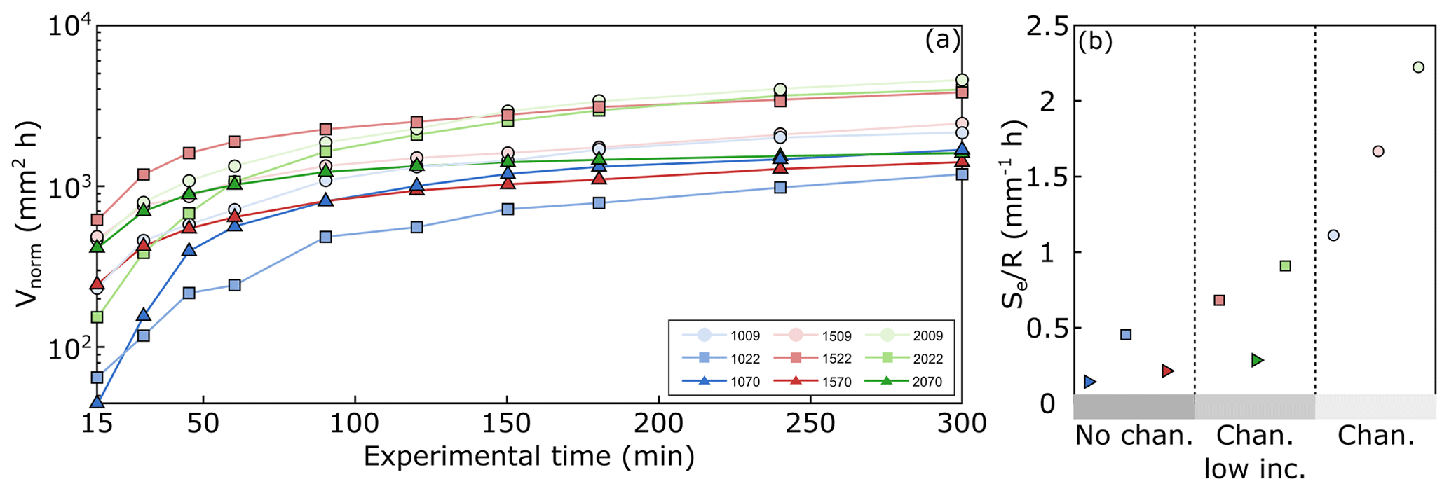
Figure 5 (a) Evolution of the normalized volume (V_norm) by imposed slope and rainfall rate for all the models. (b) $S_{\mathrm{e}}/R$ in controlling the development of channelization (No chan.: no channelization develops; Chan. low inc.: development of channelization with low incision; Chan.: channelization develops).

Figure 5b clearly shows the relationship between the imposed boundary conditions – imposed slope (S_e) and rainfall rate (R) – and the evolution of the models. We group the models into three main landscapes, following the rainfall rate.

• i.

  When $S_{\mathrm{e}}/R$ is lower than 0.5 (dark gray, Fig. 5b), channelization is less important than diffusive processes in controlling the erosion. Models with high rainfall rate (mod1070, mod1570, mod2070) or low rainfall rate and low imposed regional slope (mod1009) show low channelization with respect to the other models. Even if mod1009 shows channelization in its DEMs (Fig. 2a), the level of incision (Fig. 2b) shows that erosion is broadly distributed and not concentrated in channels or valleys so that detachment-limited conditions for channel incision do not apply.

• ii.

  When $S_{\mathrm{e}}/R$ is comprised between 0.5 and 1 (medium light gray, Fig. 5b), channelization processes are present and are responsible for the erosion. Still, channels and valleys are wide (ca. 6 cm) with respect to models where $S_{\mathrm{e}}/R$ is higher than 1 (mod1009, mod1509, mod2009; light gray in Fig. 5b).

• iii.

  In these latter cases, channelization is the main process in controlling erosion. The maximum incision rate is lower than 20 mm h⁻¹ (Fig. 3b), and the eroded volumes range between 0.1 and 0.75×10⁶ mm³.

The only exception for this trend is mod2070, which should fall into the “no channelization” landscape. Mod2070 is classified as “channelization with low incision” landscapes instead. We previously described how the extremely high R is partly balanced by a very high S_e so that even if the rainfall rate guides the model toward the “no channelization” landscape, the imposed slope promotes enough potential energy to allow the formation and the development of channels, even with low incision (Fig. 2b). It is then clear that a threshold for channelization exists. This threshold is modulated mainly by the rainfall rate, but also by the imposed regional slope. We propose that $S_{\mathrm{e}}/R$ can be used as a threshold parameter to define if and how channelization processes may develop in analog models as an indicator for the applied boundary conditions.

The applied boundary conditions are needed to constrain the reliability of analog models in understanding the evolution of natural prototypes. The possibility of applying scaled data from analog models to natural landscapes is reliant on the boundary conditions. For example, the extremely high rainfall rate used in this work is difficult to compare with nature.

4.2 Geomorphological metrics in analog models and natural prototypes

The concavity index θ of the selected channels (for every model) is usually lower than 0.4 (values between the 25th and 75th percentile; Fig. 1c). The lower values of θ are related to straight longitudinal channel profiles (Fig. S2) that are established over the course of a model run (Duvall et al., 2004; Reitano et al., 2020; Whipple and Tucker, 1999). Still, θ is comparable between analog models and natural prototypes (within 0.1; Reitano et al., 2020). However, we do not normalize the steepness index k_s by a reference concavity index k_sn, as is usually done in the literature (e.g., Cyr et al., 2010; DiBiase et al., 2010; Kirby and Whipple, 2012; Lanari et al., 2020; Tucker and Whipple, 2002). This approach is used so that the steepness index directly reflects channel characteristics, without modifying the data with a normalization parameter. If n=1, there exists a linear relationship between the incision rate and k_s; i.e., an increase in the steepness index increases the incision rate and vice versa (Eq. 6). Previous works that computed values of n for different natural landscapes show that n is typically greater than or equals 1 (e.g., DiBiase et al., 2010; Harel et al., 2016; Ouimet et al., 2009), meaning that incision rates are extremely sensitive to variation in k_s of rivers in active-tectonic settings (Kirby and Whipple, 2012). In slow-tectonic settings, the incision rates show a lower sensitivity to the steepness index (Clementucci et al., 2022; Olivetti et al., 2016). For this case, we show that n has values generally lower than 1, and even negative values (Fig. 4a). Since n is dimensionless, a one-to-one comparison between models and nature is possible. The n values from our analog models are closer to estimates of n values from slow-tectonic settings compared to active domains, where n is greater than 1 (Figs. 4b and 6; Clementucci et al., 2022; Kirby and Whipple, 2012). Similar to slow-tectonic landscapes in nature, incision rates of analog models are less sensitive to variations in k_s. Moreover, the low R² (Fig. 4) testifies to a poor relationship between incision rate and k_s (n<1). Nevertheless, we observe a trend in the relationship between incision rate and k_s as a function of the applied rainfall rate (Fig. 4b). For higher rainfall rates, the incision rate increases as expected, but only with a slight increase in k_s. This consideration supports the fact that k_s plays a minor role in controlling the incision rate, like slow-tectonic natural domains.

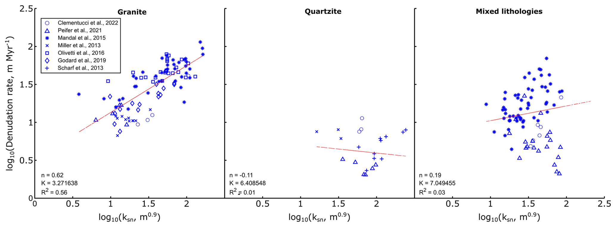
Figure 6 Logarithm of the incision rate over the logarithm of the steepness index k_sn for the selected natural prototypes (θ_ref=0.45). The linear best fit is shown by the red line. Values related to the linear regression (n and K) are shown in every plot, together with R².

Many works in the literature compute values of incision rate and k_s (or k_sn) for tectonically active regions. The models presented here are similar to natural prototypes where tectonics are absent or subordinate with respect to surface processes. To show this, we collected values of basin-wide denudation rate and k_sn (k_s normalized by the same concavity index θ_ref=0.45) for natural prototypes that show no or almost no active tectonics, divided according to the main rock types. By using this approach, we are quantifying k_sn over the denudation rate relationship and filtering it by the erodibility or rock types, as in the presented analog landscapes there is no spatial variation in bedrock erodibility. Then, we computed values of n and K (Fig. 6). Estimates of n from the analog models present a good match with data from the selected natural prototypes with slow tectonics (Fig. 6), showing values between −0.06 and 0.32 for analog models (Fig. 4) and −0.12 and 0.62 for natural systems (Fig. 6). This relationship is apparent despite the low R² value from linear regression of data from analog and natural cases. Importantly, the difference in the range of n values can likely be decreased by filtering out the basins affected by higher uplift rates within the slow-tectonic settings (e.g., granite-dominated basins; Clementucci et al., 2022). Values of K are more difficult to compare between models and nature, due to the complex dimensions that characterize the parameter (mm^1−2m h⁻¹), which require not only the application of a scaling factor but also the definition and comparison of the m variable. Since K is mainly a function of the lithology and climate (by considering uniform uplift rates; Sect. 2), and we use the same homogenous material for all the models, K only highlights the effect of the rainfall rate, and there is a nearly perfect linearity between K and the rainfall rate. For example, from 9 to 22 mm h⁻¹ and from 22 to 70 mm h⁻¹, the rainfall rate increases by a factor of 2.4 and 3.18, respectively. This is also apparent for K, with the only exception being the experiment with both moderate imposed slope and rainfall rate (mod1522). Interestingly, there is also a linear relationship between K and the slope (for example, in Fig. 4 when moving from high to low imposed slope). Although this relationship is still poorly constrained (Clementucci et al., 2022; Harel et al., 2016; Stock and Montgomery, 1999), we speculate that K is a function of not only lithologies and climate but also of the regional slope and, consequently, of the integrated topographic response to tectonic rates, as has been observed for the natural prototypes (Peifer et al., 2021).

5 Conclusions

We investigate the role of boundary conditions (imposed regional slope and rainfall rate) on the morphological evolution of nine different analog models. Some of the applied boundary conditions (i.e., the very high rainfall rate at 70 mm h⁻¹) should be considered as end-members used to fully cover the behavior of analog models under different conditions. The models systematically test various configurations of boundary conditions. We analyze how the stream power law used in natural landscapes apply to analog models, and we find that a threshold exists for the development of channelization in terms of boundary conditions ($S_{\mathrm{e}}/R$ ratio). This threshold is the result of a tradeoff between the imposed regional slope (tectonically driven topography) and the rainfall rate (climate). We find that combining imposed regional slope and rainfall rate results in three possible changes to scenarios.

• $S_{\mathrm{e}}/R$ lower than 0.5. Diffusive processes are dominant with respect to channelization so that detachment-limited conditions for channel incision do not apply (mod1070, mod1570, mod2070).

• $S_{\mathrm{e}}/R$ greater than 0.5 and lower than 1. Channelization controls the erosion of the surface, with wide channels and valleys (ca. 6 cm).

• $S_{\mathrm{e}}/R$ higher than 1 (mod1009, mod1509, mod2009). Channelization processes are the main factors controlling the morphologies of the analog landscapes.

In summary, high rainfall rates (70 mm h⁻¹) inhibit the development of channels, but not if coupled with high imposed regional slope (20^∘). Similarly, low imposed regional slope and low rainfall rate (10^∘ and 9 to 22 mm h⁻¹, respectively) develop channelization characterized by low incision. When looking at the parameterization of the stream power law for erosion, we find that analog models are described by parameters whose values slightly differ from the natural prototypes (e.g., n exponent) and by parameters that are tuned by applied boundary conditions, imposed regional slope, and rainfall rate (e.g., K coefficient). Given these findings, we propose that the insights, limitations, and range of applied boundary conditions discussed here should be considered in the future interpretation of interactions between tectonics and surface process.