the Creative Commons Attribution 4.0 License.
the Creative Commons Attribution 4.0 License.
 | 28 Sep 2023
Refining patterns of melt with forward stratigraphic models of stable Pleistocene coastlines
Paolo Stocchi
Alessio Rovere
The warmest peak of the Last Interglacial (ca. 128–116 ka) is considered a process analogue and is often studied to better understand the effects of a future warmer climate on the Earth's system. In particular, significant efforts have been made to better constrain ice sheet contributions to the peak Last Interglacial sea level through field observation of paleo relative sea level indicators. Along tropical coastal margins, these observations are predominantly based on fossil shallow coral reef sequences, which also provide the possibility of gathering reliable U-series chronological constraints. However, the preservation of many Pleistocene reef sequences is often limited to a series of discrete relative sea level positions within the interglacial, where corals suitable for dating were preserved. This, in turn, limits our ability to understand the continuous evolution of paleo relative sea level through an entire interglacial, also affecting the possibility of unraveling the existence and pattern of sub-stadial sea level oscillations. While the interpretation of lithostratigraphic and geomorphologic properties is often used to overcome this hurdle, geological interpretation may present issues related to subjectivity when dealing with missing facies or incomplete sequences. In this study, we try to step back from a conventional approach, generating a spectrum of synthetic Quaternary subtropical fringing reefs for a site in southwestern Madagascar (Indian Ocean). We use the Dionisos forward stratigraphic model (from Beicip-Franlab) to build a fossil reef at this location. In each model run, we use distinct Greenland and Antarctica ice sheet melt scenarios produced by a coupled ANICE–SELEN glacial isostatic adjustment model. The resulting synthetic reef sequences are then used test these melt scenarios against the stratigraphic record. We propose that this sort of stratigraphic modeling may provide further quantitative control when interpreting Last Interglacial reef sequences.
- Article
(3697 KB) - Full-text XML
-
Supplement
(168356 KB) - BibTeX
- EndNote


Understanding the uncertainties surrounding the rate and magnitude of ice loss from the Greenland Ice Sheet (GrIS) and Antarctica Ice Sheet (AIS; e.g., DeConto and Pollard, 2016; Edwards et al., 2019; Noble et al., 2020) is key to estimating the sensitivity of our planet to warmer climatic conditions. To better constrain these uncertainties, significant effort has been made to understand how Earth’s ice sheets have evolved during past warm periods (Tierney et al., 2020). Marine Isotope Stage (MIS) 5e, here referred to as the Last Interglacial (LIG, ca. 128–116 ka) is regarded as a process analogue for future warmer climates. In the LIG, global temperatures were 1–2 ∘C warmer and there is general consensus that the eustatic sea level was up to 1–5 m higher than present (Dyer et al., 2021). This consensus stems from geologic work on different types of sea level indicators found along the world's shorelines (Rovere et al., 2016). However, peak LIG eustatic sea level estimates vary widely, also because different locations are subject to vertical land motions that need to be accounted for before reconstructing paleo global mean sea level (GMSL) from field data. These post-depositional processes include glacial isostatic adjustment (GIA), sediment loading, subsidence, tectonics, and dynamic topography (Creveling et al., 2015; Simms et al., 2013; de Gelder et al., 2020; Malatesta et al., 2022; Austermann et al., 2017).
A further challenge resides in interpreting, within fossil LIG coastal sequences, short-lived sea level oscillations or sudden accelerations. In the granitic Seychelles, for example, isolated in situ MIS 5e corals have been sampled and surveyed 8 m above mean sea level (a.m.s.l.) with similar facies found directly offshore in the modern intertidal (Dutton et al., 2015). Previous lithological descriptions by Montaggioni and Hoang (1988) and a detailed modern investigation by Vyverberg et al. (2018) suggest that alternating reef sequences and coral rubble/coralline algae layers could represent a step-wise increase in sea level throughout the LIG. However, these are isolated pockets of preserved reef material, and it is uncertain as to whether this sequence is derived from short-term environmental change (e.g., wave climate, coral bleaching, increased sediment input) or if indeed it is evidence of a broader series of sea level rise and stillstand events within the LIG. Off the western coast of Australia, O’Leary et al. (2013) found evidence of a slow increase in sea level before a 9 m a.m.s.l. peak at the end of the LIG. Recent reevaluation of sea level indicators in the Bahamas show a significantly lower eustatic sea level (1.2–5.3 m, 95 % confidence interval) with an initial peak and no evidence of a late-LIG peak (Dyer et al., 2021). Empirical attempts have also been made to extract global LIG sea level patterns, for example, Kopp et al. (2009) provide a statistical approach to integrate existing individual sea level indicators into a global model based on probability densities and produced a probable “double-peak” eustatic curve with both an early and late peak in LIG sea level. Such sudden dynamism in LIG sea level cannot be identified in ice proxies, such as pollen records and ice-rafted debris (e.g., Barlow et al., 2018).
Unfortunately, solutions to this dilemma are dependent on the facies that are preserved and their geographic distribution in any given region. Unlike late Holocene studies in the tropics, where nearshore seismic and drilling campaigns on coral reef slopes can synthesize broad lithostratigraphic sequences, Pleistocene studies usually rely on either poorly preserved or spatially limited emerged reefs. Due to the inaccessibility of most emergent reef complexes, methods other than land-based seismic surveying and drilling are needed in order to supplement field observations and test interpretations.
One potential solution lies in the use of forward stratigraphic models (FSMs). Over the last 2 decades, a suite of 2D and 3D carbonate-specific FMSs have been developed either to aid in petroleum exploration (large, basin scales) or in recent Quaternary investigations (small, reef-specific scales). These include CARB3D+ (Warrlich et al., 2002, 2008; Barrett and Webster, 2012), pyReef-Core and BayesReef (Salles et al., 2018; Pall et al., 2020), ReefSAM (Barrett and Webster, 2017), and Dionisos (Granjeon et al., 1999). While each model has individual merits, Dionisos has proven to be consistently robust in predicting intermediate-scale reef development over the Quaternary (Seard et al., 2013; Montaggioni et al., 2015). Building on the success of Montaggioni et al. (2015) to model tropical atoll development through the Quaternary, this study aims to explore the late-LIG sea level jump conundrum through the application of a suite of GIA models to fringing reef inside Dionisos. Here, we take an idealized version of the modern fringing reef system observed offshore southwestern Madagascar and subject it to glacial/interglacial cycles starting at 400 ka, before deviating from the baseline model at the start of the LIG. Resulting 3D shorelines and synthetic well logs aim to re-evaluate sub-stadial melting patterns previously interpreted from outcrop evidence in Boyden et al. (2022).
This study uses Dionisos (OpenFlow Suite, v. 2021.1, Update 4, BieicipFranlab, 2021) from IFP Energies nouvelles and Beicip-Franlab to synthesize a suite of emergent LIG coral reef terraces along the southwestern coast of Madagascar, at the Lembetabe site. In order to test the sensitivity of the geological record to changing sea level conditions, we model three distinct relative sea level scenarios extracted from a coupled ANICE–SELEN model.
2.1 Study area
Lembetabe sits along the remote southwestern coast of Madagascar (Fig. 1a). Surrounding the small fishing village, semi-vegetated rolling dune fields back a well-preserved LIG reef sequence that sits several meters above a modern wide fringing reef (see Boyden et al., 2022, for stratigraphic and geomorphic description). Additionally, situated on a stable coastline since the Eocene, and in the far-field of Quaternary ice sheets, Lembetabe provides an excellent opportunity to examine more subtle changes in eustatic sea level (Du Puy and Moat, 1996).
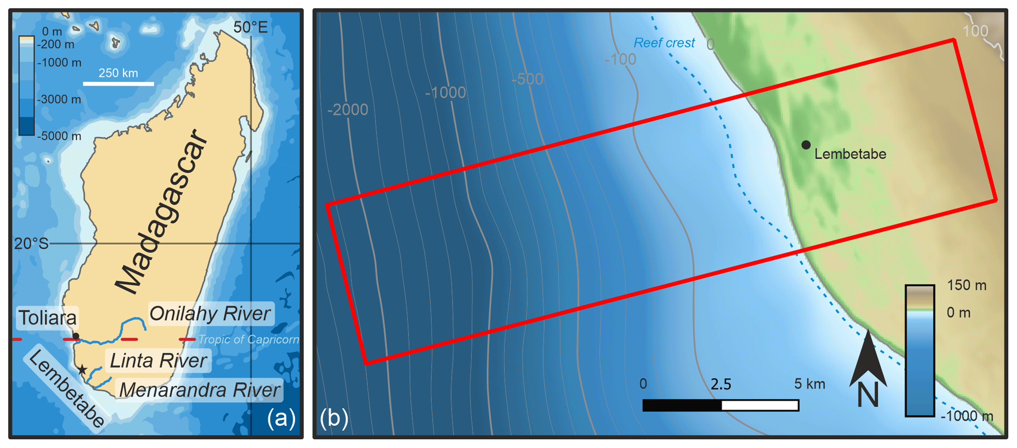
Figure 1(a) Overview map of Madagascar, the study area at Lembetabe, and the three rivers in the southwest of the island. Map data from Natural Earth. (b) Overview of Dionisos model domain with combined topography/bathymetry detailed in Sect. 2.2.
2.2 Topography and bathymetry generation
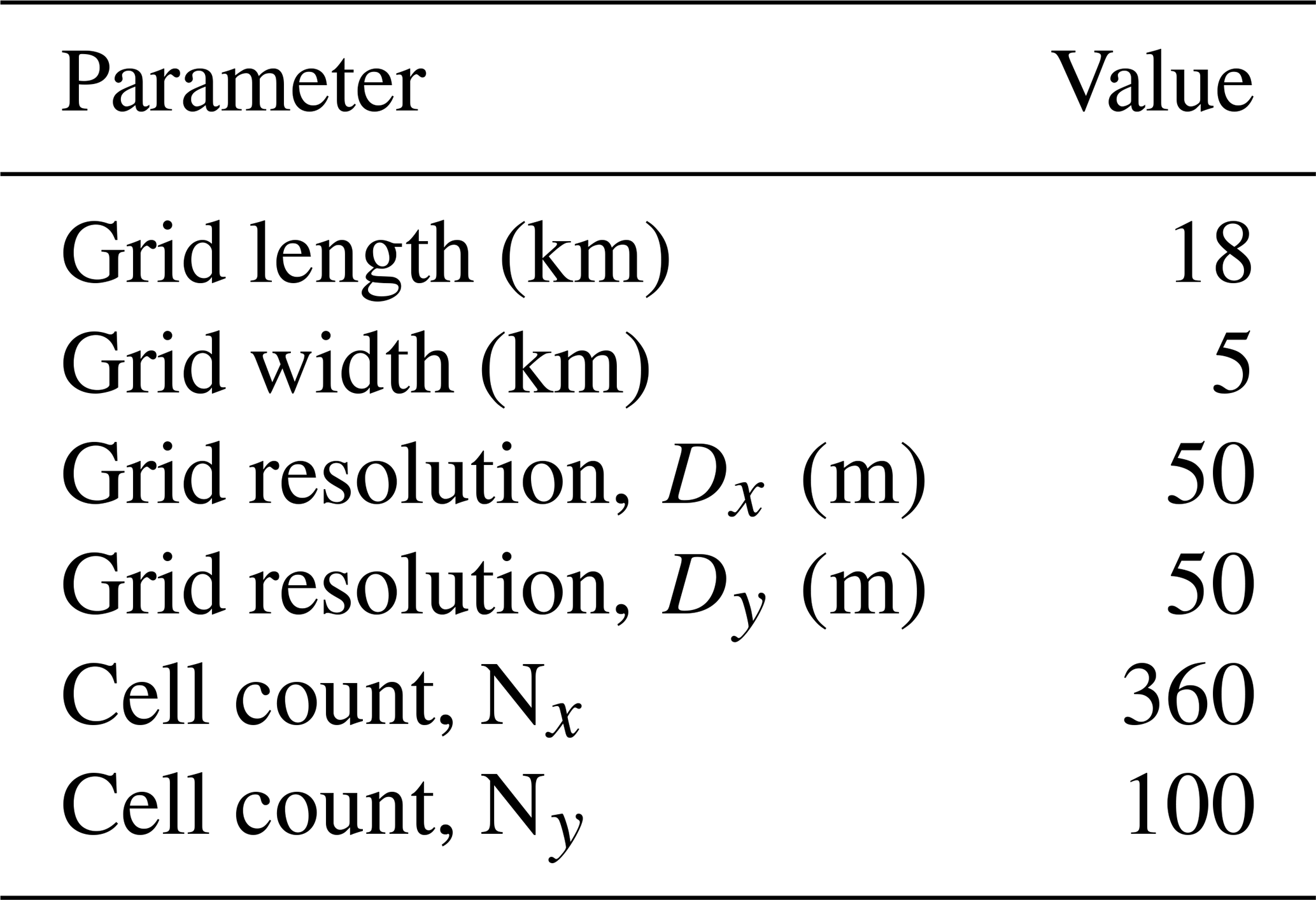
Unlike subsiding coastlines like the Mururoa Island atoll investigated in Montaggioni et al. (2015), Lembetabe's emergent fringing coral reef has not been subject of extensive coring or seismic campaigns, and therefore no high-resolution nearshore bathymetry or subsurface horizons exist. In order to address this, we derived a high-resolution (120 mm px−1) land digital elevation model (DEM) from aerial-based Structure from Motion/Multi-View Stereo (see Boyden et al., 2022, for methodology and processing description) that has been merged down to TanDEMx topography at 30 m resolution (© DLR 2021). In order to capture the fringing reef, we extracted the modern nearshore bathymetry at Lembetabe from WorldView 2 satellite imagery (v. 28.4, May 2020) using the SPEAR Relative Water Depth toolset within ENVI® (v. 5.3.1). This bathymetry dataset was previously calibrated by Weil-Accardo et al. (2023) using sonar soundings obtained with a Deeper Smart Sonar Pro™ (https://www.deepersonar.com, last access: 10 November 2021) sonar unit. These depth transects were then corrected to the established local mean sea level tidal datum from Boyden et al. (2022) before being used for the absolute depth calibration step in the ENVI toolset. Topography, nearshore bathymetry, and the much coarser-resolution GEBCO database offshore bathymetry (https://download.gebco.net/, last access: 20 November 2021) were resampled with cubic convolution in Surfer (Golden Software, v. 21.2.192), where artifacts from the merging process were corrected and then the entire DEM was exported to the final 50 m × 50 m model grid resolution (Fig. 1b). Once exported, the decimated DEM was imported into the Dionisos environment where a 18 km × 5 km domain was centered at Lembetabe. This domain was then rotated 15∘ from the horizontal so that the shoreline runs approximately horizontal through the gridded domain. By doing this, intra-grid incident angles during wave propagation calculations can be minimized (e.g., Roelvink et al., 2009). Final model domain patterns are summarized in Table 1.
2.3 Sediment classes
In order to resolve complex reef environments, Dionisos utilizes user-defined sediment classes. Each sediment class is determined through four parameters: (1) type of sediment (carbonate, clastic, evaporate, etc.), (2) grain size, (3) solid density, and (4) burial compaction law (observed or mechanical). In this model, we classify the seven sediment contributors: five coral-specific classes that follow the same system used in Seard et al. (2013), a standard carbonate sand class, and a standard carbonate mud class (Table 2). The initial sediment class distribution is defined by the substratum constituents. Here, the substratum, referred to as “Basement”, is an equal distribution of the coral sediment classes and is set to a thickness of 20 m. This is an approximation for the region as no borehole data exist. Furthermore, to the east of Lembetabe is a 30 m high limestone escarpment of Eocene Epoch, suggesting the basement in the region is limestone as well (Battistini, 1964; Du Puy and Moat, 1996).
Table 2Sediment classes used within Dionisos. Coral-related class parameters are the same used in Seard et al. (2013).
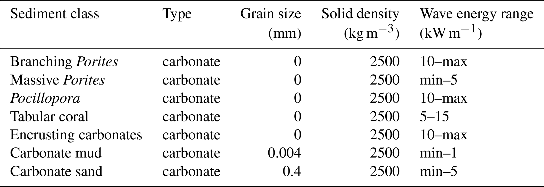
As described by Boyden et al. (2022), sediment along the Lembetabe coast is dominated by carbonate with little siliciclastic component, and therefore no fluvial clastic component is included in the model. It should be noted that during glacial periods, increases in precipitation in the hinterland could occur and an influx of clastic sediment could enter the system, but these are ignored for the goals of this investigation. While de-watering of compacting sediments in siliciclastic systems can have large effects on the overall water budget (Revil et al., 2002), carbonate-dominated systems have much more varied porosity that is subject to significantly more alteration during the early stages of burial (i.e., diagenesis, Lee et al., 2021). The overall reef architecture and therefore ensuing framestone lessens the changes in pore space at shallower burial depths, and therefore we treat the reef “sediment” compaction as negligible. However, resulting sand and debris facies are governed by a simplified mechanical compaction that is linear to depth. Finally, while Dionisos has the ability to include fluvial input, this is also treated as negligible as the three rivers in the region, the Onilahy (140 km to the north), Linta (30 km to the southeast), and Menarandra (70 km to the southeast), flow sporadically throughout the year and are unlikely to have provided significant sediment loads to the system (Fig. 1b).
2.4 Hydrodynamics
Dominant wave direction and magnitude have significant influence on shoreline geometry as well as the ability of coral colonies to flourish (Gischler et al., 2019). Dionisos quantifies this impact by calculating wave energy and refraction based on Snell's law:
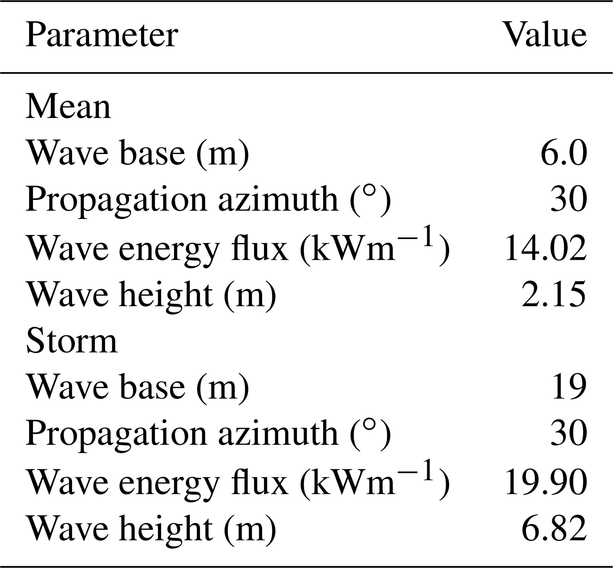
where βd is the wave angle in deep water, βs is the wave angle in shallow water, Cd is the wave velocity in deep water, and Cs is the wave velocity in shallow water (Holthuijsen, 2007, e.g.,). In order to address this, the mean observed significant wave height (Hs) and direction were extracted from the Centre for Australian Weather and Climate Research (CAWCR) global hindcast raster (Durrant et al., 2013). This global wave hindcast was extracted from the WaveWatch III wave model over 1979–2010 in a 0.4∘ × 0.4∘ global grid. The resulting values from the grid cell overlaying Lembetabe were then extracted as hydrodynamic boundary conditions for the model.
In addition to normal sea state conditions, storms play a crucial role in coral reef development and colony long-term stability (Gardner et al., 2005). While the southwestern-facing shoreline of Madagascar is generally sheltered from approaching tropical cyclones spawning in the Indian Ocean, category 3-equivalent Tropical Cyclone Haruna spawned in the Mozambique Channel and made landfall at Toliara, approximately 150 km north of the study site (Côté-Laurin et al., 2017). Therefore, to approximate for storm impacts, the maximum significant wave height from the CAWCR model was extracted and added to the model at a 10 % yearly occurrence rate. The wave parameters are summarized in Table 3.
2.5 Carbonate production and facies identification
Carbonate production is naturally the largest variable in a carbonate forward stratigraphic model. Several factors directly control the dominate coral species and rate of growth: water temperature, turbidity, wave energy, and water depth (e.g., Montaggioni and Braithwaite, 2009). In order to address this, Dionisos classifies each carbonate producer under the four component sediment class definitions from Sect. 2.3 and then adds a user-defined production-versus-depth value to each carbonate sediment class. This production-versus-depth curve represents the non-linear relationship between carbonate producer growth rate and depth. To streamline this process, Dionisos provides growth curves for several frequently used carbonate sediment classes as defined in the literature.
For the purposes of this study, we utilize the growth curves described by Montaggioni et al. (2015) for our coral-based facies, the tabular coral growth curve from Lanteaume et al. (2018), the encrusting coral growth curve from Kolodka et al. (2016), and the carbonate sand and mud curves from Burgess and Pollitt (2012). In the model, production is controlled as either a constant or is linear per time interval. For example, Montaggioni et al. (2015) experimented with varying the growth rates through time and achieved significantly different results. However, because for Lembetabe we lack the seismic data and well logs available to Montaggioni et al. (2015), our simulations are run with constant maximum growth rates from the literature mentioned above, e.g., 2500 m Myr−1 for coral facies, 1500 m Myr−1 for encrusting carbonates, 2000 m Myr−1 for tabular corals, and 1000 m Myr−1 for carbonate sand and carbonate mud throughout the model run (Fig. 2).
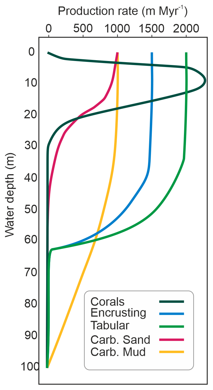
Figure 2Production rate (m Myr−1) as a function of water depth for each sediment class included in the Dionisos model.
2.6 Sediment weathering
A significant limitation in the use of geological proxies to investigate intra-stadial sea level fluctuations is a reliance on the preservation of the target sequence. This becomes especially challenging when the target sequence is within the dynamic coastal zone. For example, Malatesta et al. (2022) demonstrates how overprinting can lead to ambiguities in erosional rates and inferred uplift rates of coastal terraces. Within the Dionisos environment, four forms of weathering are taken into account: (1) maximum subaerial weathering rate, (2) maximum weathering decay in the marine environment, (3) dissolution rate, and (4) transformation rate. Maximum weathering rates for exposed limestone are hard to quantify (Enos and Franseen, 1991). This is because the rate is heavily dependent on post-depositional environmental factors like precipitation, porosity, and groundwater chemistry. To approximate for this, Montaggioni et al. (2015) used a 250 m Myr−1 that was measured by Trudgill et al. (1979) using micro-erosion meters on Aldabra, the Seychelles. However, in the case of Lembetabe, mean annual precipitation is well below that seen on Aldabra or Mururoa (> 1000 mm vs. 62 mm) and subaerial exposure is more likely to be well below the one found in more tropical localities. Therefore, we utilize a maximum subaerial weathering of 100 m Myr−1. To quantify the mechanical and biological erosion under marine conditions, we use a maximum 100 m Myr−1 weathering rate (between the lower and the average values, 0 and 1000 m Myr−1, respectively, used by Paulay and McEdward, 1990). To simplify the computational load, the dissolution rate was incorporated within our maximum subaerial erosion rate. Finally, the transformation rate allows for the conversion of mass from deposited carbonate into carbonate sands and muds. Within Dionisos this is treated as a constant rate and was set to the standard value of 50 m Myr−1 for each sediment class, except for carbonate sand and carbonate mud.
2.7 Glacial isostatic adjustment
Accommodation space is the final governing factor in reef development and morphology (Woodroffe, 2002). As sea level rises and falls, the relatively habitable window for corals moves, sometimes drastically, shifting the area of reef growth either up or down the coastal profile (Camoin and Webster, 2015). As described before (Sect. 1), beyond ice sheet mass balance, post-depositional processes can significantly affect relative sea level (RSL) through glacial/interglacial cycles. Generally, this comprises GIA, dynamic topography, tectonics, and other vertical land motion processes. In southwestern Madagascar, the coastline is considered to have been tectonically stable since at least the Eocene; therefore GIA was treated as the primary post-depositional influence. To take this into account we utilize solutions from a coupled ANICE–SELEN model (Bintanja and van de Wal, 2008; de Boer et al., 2013, 2014). When coupled together, the ANICE model provides the 3D ice sheet extents for North America, Eurasia, Greenland, and Antarctica to the SELEN model at 1000-year time steps, which then calculates the redistribution of water mass and deformation of the solid Earth (de Boer et al., 2013; Spada and Stocchi, 2007). Once calculated, SELEN sends a new RSL and deformation back to ANICE in order to solve the next time step. The final output is an RSL curve that incorporates the GIA signal for a defined geographic location.
2.8 Scenarios and testing
In order to test the two prominent GrIS and AIS melt patterns within Dionisos, we extracted three RSL scenarios from the ANICE–SELEN model for the last 410 ka: one baseline scenario and two scenarios where RSL changes over 130–115 ka (Fig. 3a). The initial Dionisos model run was driven by an RSL curve where ice sheets are held to modern geometries at the beginning of the LIG (Fig. 3b). By halting the melting of both GrIS and AIS, the resulting signal is the background GIA response. This background GIA scenario is referred to as “Baseline” and has a peak sea level of 2.11 m a.m.s.l. at 126 ka. The second scenario, “Full”, represents an initial simultaneous collapse of GrIS and AIS, contributing 2 and 5 m, respectively (Fig. 3c). This second scenario produces an early peak of sea level of 8.33 m a.m.s.l. by 125 ka, followed by a relatively stable, gentle regression. An early peak, driven by continental levering and ocean syphoning, has often been seen as the classic LIG fingerprint in the far-field (e.g., Barlow et al., 2018). In the third scenario, “G2A5”, the contributions from GrIS and AIS are separated, creating a two-peak LIG sea level history. Here, GrIS melts first and contributes 2 m to sea level rise over 126–124 ka that produces the initial peak of 3.55 m a.m.s.l. Following a stable period in sea level, AIS begins to melt at 118 ka and contributes 5 m to sea level rise late in the LIG, producing a second, higher peak sea level of 6.43 m a.m.s.l. (Fig. 3d). This scenario represents possible discrepancies in GrIS–AIS stability and variable hemisphere-specific climate fluctuations (e.g., Govin et al., 2012; Stone et al., 2016), and it is consistent with the interpretation of fossil reef sequences from Western Australia described by O’Leary et al. (2013).
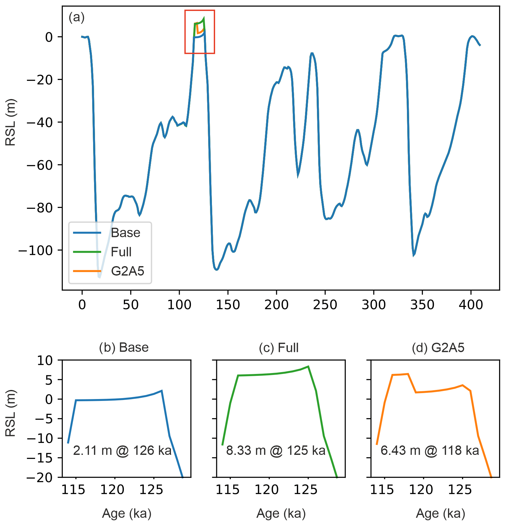
Figure 3RSL sea level curves extracted from ANICE–SELEN for Lembetabe and used in Dionisos. (a) Overview of RSL over 400–0 ka. (b) Baseline curve with no further melting of GrIS or AIS beyond modern geometries at LIG. (c) Full RSL curve, with joint melting of GrIS (2 m) and AIS (5 m) at the onset of the LIG. (d) G2A5 RSL curve, with initial 2 m contribution from GrIS, followed by a later contribution of 5 m by AIS. Magnitude and timing of peak RSL in each scenario is included for reference.
The Dionisos model was first run under Baseline forcing. This was done in a three-segment process where the model was run at 10 kyr time intervals over 400–150 ka. At 150 ka, the time intervals were reduced to 1 kyr intervals until 80 ka. Then, over 80–0 ka, time intervals were increased to 5 kyr. This modulation of time intervals allowed for the reduction in computational demand while emphasizing the LIG. Following the completion of models for each mantle viscosity under Baseline conditions, the Full and G2A5 scenarios were run from the Baseline 150 ka time step. This iterative process is summarized in Fig. 4.
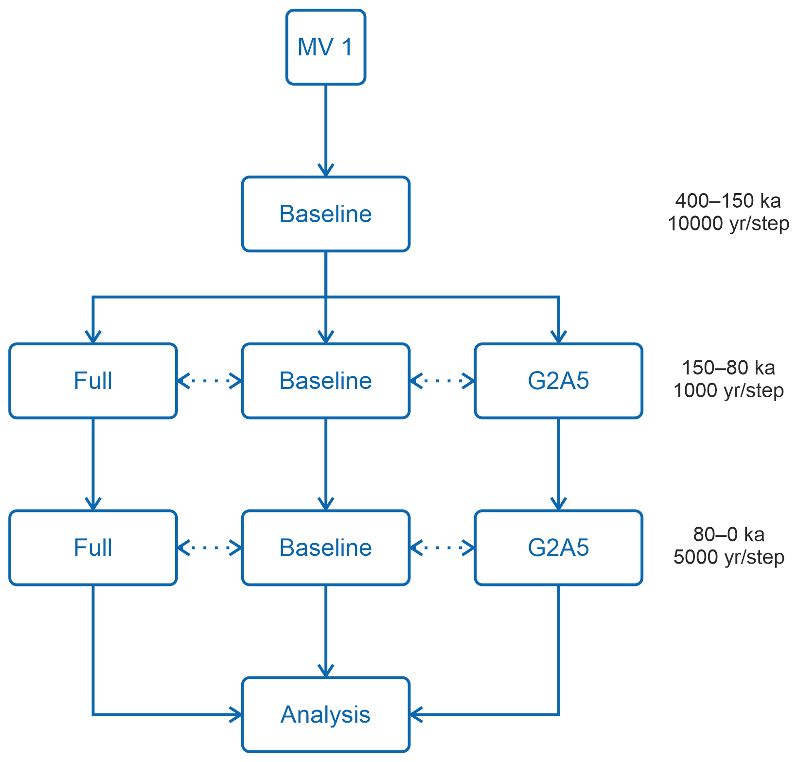
Figure 4Outline of experimental design. MV 1 represents the mantle viscosity scheme used during the ANICE–SELEN model calculations. “Full” represents an early LIG peak in sea level that is driven by simultaneous melting of GrIS and AIS, contributing 2 and 5 m, respectively. “Baseline” is the background GIA signal during the LIG, where ice sheets are kept to modern geometries throughout the LIG. “G2A5” is a two-step LIG scenario where GrIS melt adds 2 m to sea level at 125 ka followed by a brief plateau before AIS melt contributes 5 m at 118 ka.
2.9 Model caveats
As with any model environment, certain limitations arise when transferring the physical environment into the virtual, often leading to an oversimplification of complex physical systems. The model used in this study is not an exception. Within the scope of this study, the primary interest is to evaluate shallow water reef evolution through glacial/interglacial cycles. Dionisos solves sediment transport between cells using a diffusion equation (Granjeon et al., 1999). As pointed out by Barrett and Webster (2017), this simplification works well for large-scale, basin-wide models but fails to capture the more nuanced hydrodynamics within shallow reef environments. In order to address this without redesigning the entire Dionisos architecture, characterization of the nearshore wave environment allows for a reasonable approximation at our model grid resolution of 50 m × 50 m.
The largest caveat however, is the method in which Dionisos solves for subaerial erosion. This is partially addressed through the use of user-defined weathering rates for each sediment class. However, in Lembetabe, modern active dune fields and fossilized aeolianites cover MIS 5e reefs, suggesting extensive offshore migration of dunes during glacial periods (e.g., Battistini, 1965; Boyden et al., 2022). The speed at which active dunes migrate would limit the overall exposure time of previously deposited limestone (Bristow et al., 2005). In order to try and limit the overestimation of subaerial weathering, we employ a lower weathering rate than regularly cited for coastal limestone facies (e.g., 100 vs. 250 m Myr−1, Trudgill et al., 1979).
The results from the Dionisos model are organized two fold in the following section. First, transgression and regression timings for each scenario are described. Second, in order to better visualize the differences between the sea level scenarios adopted, three synthetic wells were created along a cross-platform profile within the baseline model output. The first (Well A) is located just before the continental-shelf break, the second (Well B) is within the reef, and the third (Well C) is located in the intertidal. Well locations can be seen in Fig. 6.
3.1 Facies deposition
Within the post-processing model environment, seven facies were declared following the coral distribution scheme laid out by Montaggioni (2005) for reef-dominated coasts in the Indo-Pacific basin as well as model-specific environmental constraints from Seard et al. (2013). The relationships between sediments and environmental controls within the model output are summarized in Fig. 5. Each facies is a combination of one or more of the sediment classes described before (Sect. 2.3) and deposition depth. Further classification parameters are possible but are beyond the scope of this study and require significant fine-tuning. Moving from off-shore over the reef, we noted (1) forereef, (2) reef crest, (3) reef flat, (4) bypass, (5) beach, (6) basement, and (7) unclassified. Applying the declared facies to each scenario, the following depositional histories were obtained for each scenario at each well location.
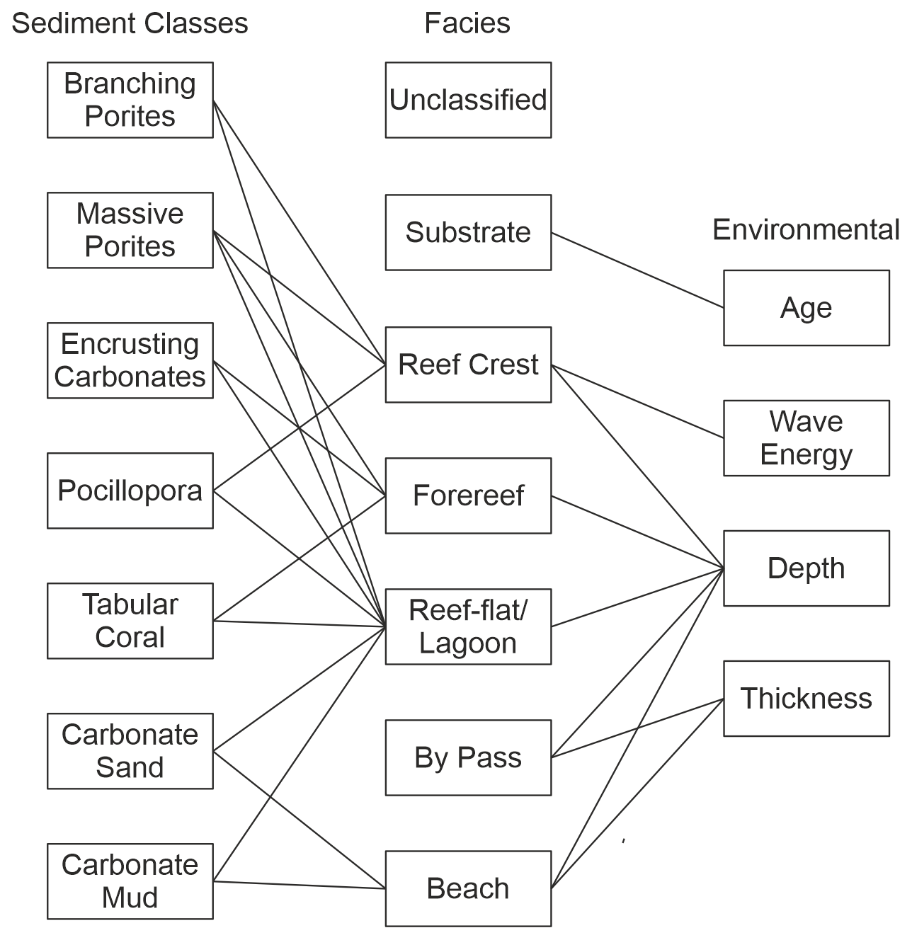
Figure 5Identification pathways for determining facies within Dionisos. Adapted from Montaggioni (2005) and Seard et al. (2013).
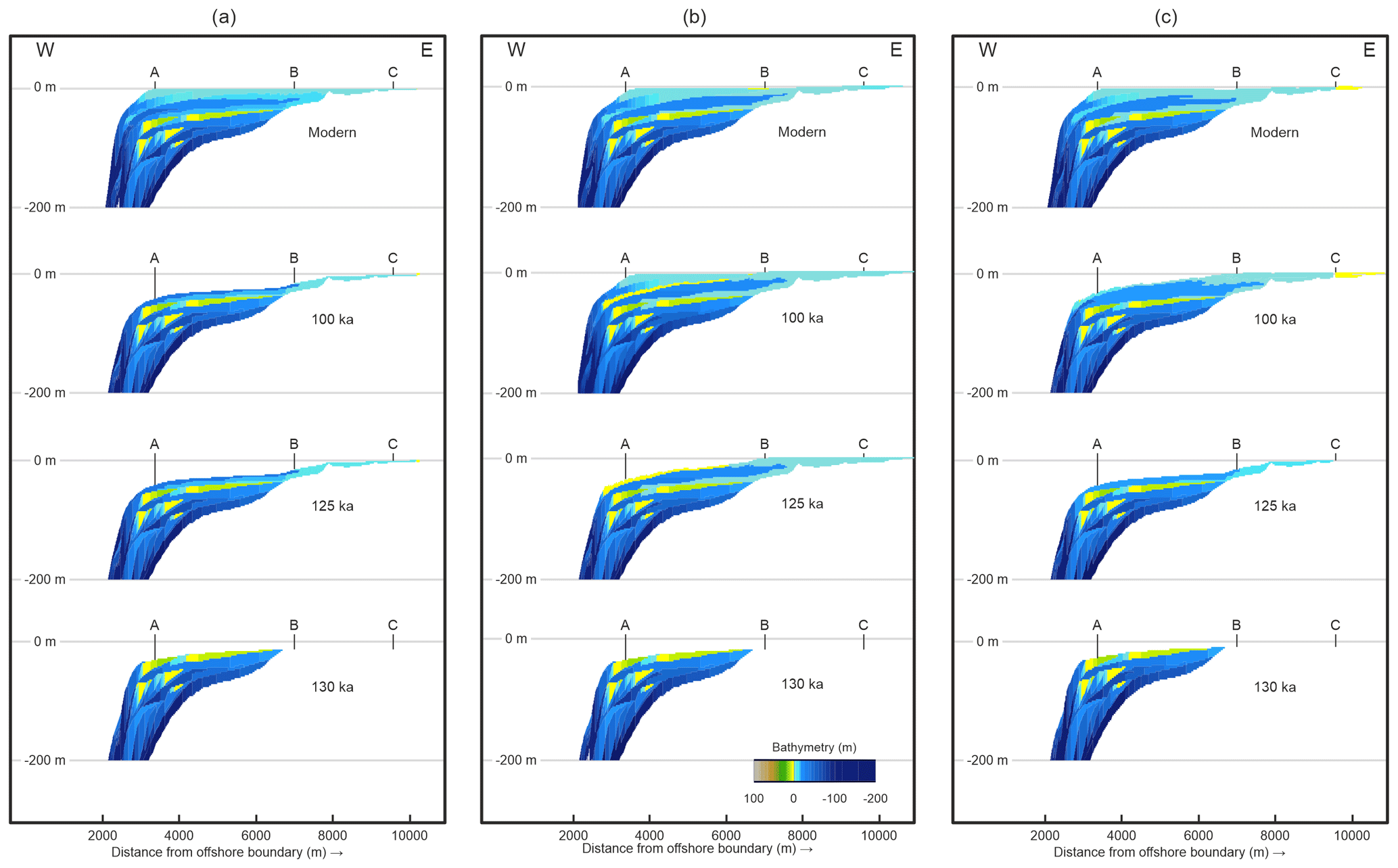
Figure 6Dionisos model output for major event markers: 130 ka, 125 ka, 100 ka, and modern. (a) Baseline model driven by background GIA, (b) Full model incorporating simultaneous melting of GrIS and AIS, and (c) G2A5 model subjected to initial GrIS melting followed by AIS melting near the end of the LIG.
3.1.1 Baseline
Well A, sitting near the edge of the platform, first registered transgression at 131 ka with the initiation of a 2 m thick reef crest. Sea level continued to rise with the back-stepping of the reef crest and subsequent deposition of a forereef sequence over 130–115 ka. Sea level began to fall and hydrodynamic conditions allowed for a second reef crest sequence, 4 m thick, to be deposited. By 110 ka, the sea level had regressed back beneath the platform edge, leaving the LIG exposed and subject to weathering. Burial analysis of the sequence shows that the upper 7.5 m of LIG limestone was eroded, leaving the 116 ka forereef unit as the highest remaining LIG unit in the resulting lithostratigraphy (Fig. 8a). At 15 ka there is again transgression of the platform and rapid deposition of a 13.9 m thick sequence of forereef by 5 ka.
At Well B, midway on the platform, the Baseline model shows rapid flooding starting at 130 ka. Over 129–122 ka, a 23.3 m thick sequence of reef crest was deposited. This was followed by a 3 m sequence of an unclassified facies, most likely a reef flat-like sequence that did not match the previously defined parameters (Fig. 5). The unclassified sequence was capped off by a thin beach deposit by 120 ka. This beach deposit was a thin veneer that reached no more than 0.5 m thick and covered the LIG reef crest sequence over 120–88 ka. Subaerial erosion began taking place, eroding 3.5 m from the uppermost part of the LIG sequence by 10 ka. At that point, the sea level transgressed again, depositing a 1.5 m-thick Holocene reef crest that was subsequently covered by an equally thin Holocene reef flat deposit.
Well C occupies the modern intertidal. The baseline LIG sea level transgression reached the well at 127 ka. The relatively stable nature of the background GIA signal at Lembetabe created a prograding fringing reef. Here, a 1 m-thick sequence of reef crest was deposited over 127–126 ka. This reef crest sequence was followed by a reef flat sequence 2.5 m thick over 126–125 ka. As sea level continued to recede, a 1 m thick sequence of alternating beach and unclassified units were deposited. By 124 ka, the sequence was left exposed and the upper 2.5 m of the sequence was eroded away before the Holocene transgression at 10 ka. The Holocene transgression deposited further reef flat units on top of the LIG up to modern sea level.
3.1.2 Full
The platform edge under the combined GrIS and AIS “Full” scenario is initially flooded at 131 ka. A quick initial pulse of forereef deposition occurring over 130–125 ka resulted in a 9 m thick unit. Deposition slows up until peak sea level is reached at 120 ka, after which sedimentation rates increase as sea level falls again. This leaves behind a 3 m thick unit of forereef over 120–113 ka. As sea level continues to fall, a 3.5 m reef crest unit is deposited in the remaining accommodation space by 111 ka, before the platform becomes emerged and a thin 0.5 m beach unit is deposited on top. The uppermost 10 m of the LIG are then eroded away during the intervening subaerial exposure. At 15 ka, the Holocene transgression reoccupies the platform and 18 m of forereef is deposited on top of the remaining LIG over 15–5 ka. Following 5 ka, the sea level begins to slightly recede, allowing for the deposition of a 15 m thick reef crest unit.
Similar to the platform edge, transgression during the LIG begins by 130 ka with an initial 0.5 m thick reef crest unit. This is then quickly covered by forereef units interbedded with unclassified sediments as sea level continues to rise until 125 ka. In total, 25.3 m of forereef and unclassified sediments accumulate before sea level begins to fall. Over 125–119 ka, an additional 1 m of forereef sediment accumulates before conditions are conducive for the deposition of 2.9 m of reef crest. Sea level drops yet further and a final phase of sedimentation sees 1.2 m of reef flat before a final veneer of beach is deposited by 116 ka. The section becomes emerged and undergoes subaerial erosion until 10 ka, eliminating the upper 8.5 m of the LIG sequence. The final Holocene sequence comprises 1.4 m of reef flat topped with a shallow-water unclassified sediment that reaches the present-day sea level.
The LIG for Well C under the full scenario produces an initial inundation at 127 ka when a 10 cm thick unit of reef crest was deposited. This is followed by additional sea level rise and the deposition of a 3.5 m thick forereef unit by 125 ka. Following this, accommodation space is decreased and a 4.4 m thick reef crest unit is deposited. Further shallowing and progradation cause the deposition of a final 1.8 m thick sequence of reef flat and 0.8 m thick shallow-water unclassified sediment unit by 122 ka. This was left subaerially exposed and the uppermost 3.5 m of the LIG eroded, leaving the remaining LIG reef crest exposed at +3.5 m a.m.s.l. (Fig. 8c).
3.1.3 G2A5
Transgression over the platform edge begins at 132 ka under the G2A5 scenario with the deposition of a 1 m thick reef crest. Rapid sea level rise causes back-stepping of the reef made evident by the deposition of a 9 m thick reef crest occurring over 131–125 ka, coinciding with the GrIS melt contribution. At 125, RSL begins to decrease, eroding the upper 1.5 m of the earlier-deposited reef crest by 119 ka. AIS melting influence is then gradually felt, again slowly depositing a reef crest unit over 118–113 ka. By 113 ka, rapid increase in sea level is seen and 2.5 m of further forereef are deposited by 110 ka. As sea level regressed, a 5.6 m thick sequence of reef flat and unclassified units were deposited over 110–109 ka. Finally, the LIG sequence was covered by interbedded beach and unclassified deposits reaching a maximum of 8.8 m thick, as sea level fell back beyond the edge of the platform.
At Well B the LIG sequence begins at 130 ka with the deposition of a 0.5 m thick reef crest unit. This is then covered by the rapid deposition of 33.3 m of reef flat over 127–116 ka, again coinciding with GrIS melt contributions. It should be noted that this peak deposition is greater than 5 m above modern sea level. Following the initial peak in sea level, Well B is left exposed and 17.1 m of previously deposited reef flat is eroded by 80 ka. Erosion continues until the onset of the Holocene, when 10.3 m of reef crest is deposited by 5 ka and a final 3 m thick unit of reef flat is deposited up until the present day.
Finally, Well C records the initial LIG transgression at 126 ka. This comprises a 4.6 m deposit of reef flat by 124 ka. Above the reef flat, a 0.5 m thick beach unit is deposited by 123 ka but is subsequently partially eroded during the intra-peak regression. AIS-driven sea level rise re-inundates the intertidal and deposits a 2.8 m thick unit of reef flat over 119–117 ka. A final 0.8 m thick beach unit is deposited atop the LIG sequence by 116 ka. As at Well B, rapid regression occurs and the entirety of the LIG sequence is eroded away. Reoccupation of the platform at 10 ka, deposits a final 2 m thick unit of reef flat that is visible in the final litholog (Fig. 8c).
This implementation of Dionisos focuses on two commonly cited scenarios (e.g., Barlow et al., 2018; O’Leary et al., 2013) for GrIS and AIS melt contributions to the LIG by comparing the fringing reef accretion under the respective GIA-derived RSL curves against a reef sequence created using a pure background GIA RSL history. Our results show distinct differences in nearshore reef accretion during the LIG as well as stark differences in the preservation of LIG in the modern stratigraphy under different ice sheet melt scenarios. In the following we (1) quantify the differences in accretion, (2) examine preservation shortcomings, and (3) evaluate the applicability towards real-world LIG fossil reef-based studies.
The two main direct consequences of changes in ice sheet melting parameters are changes in the amplitude and duration of maximum inundation. This has direct influence on the overall accommodation space available for reef development (e.g., Camoin and Webster, 2015). At Lembetabe, the combined GrIS and AIS melt under the Full scenario produces a 295 % increase in RSL when compared to the Baseline, 8.33 and 2.11 m, respectively. Under the G2A5 scenario this difference is marginally less at 205 % when comparing the highest experienced sea level, 6.43 and 2.11 m, respectively. This translates to LIG water depths over the mid-platform (Well B) reaching a maximum of 17 m under Baseline, 18 m under G2A5, and 22 m under the Full scenario. The rapid flooding of the reef platform at the beginning of the LIG, would have placed the antecedent topography directly in the ideal zone of coral growth (Woodroffe and Webster, 2014). Sedimentation rates across the LIG from the mid-platform reflect this as well with rates for all scenarios peaking at around 3600 m Myr−1. Within the stratigraphy, this is recorded as both vertical accretion as well as progradation as accommodation space decreases driven by both RSL fall and reef growth (e.g., 100 ka in Fig. 6b).
By the end of the LIG, a thick carbonate package covered the platform. Under baseline conditions, maximum LIG thickness reaches 24.5 m, under the Full scenario the maximum thickness decreases to 24.1 m, and under G2A5 it decreases further to only 13.0 m. This is misleading, however, as the higher overall RSL rise during the two melting scenarios (Full and G2A5) spread accretion across the entire platform as well as further inland. This significant increase in inundated area led to a 681.5 % increase in carbonate sedimentation under the Full scenario when compared to the Baseline and a 187.5 % increase under the G2A5 scenario compared to the Baseline. The difference in carbonate package thickness between the Full and G2A5 scenarios is driven by the duration, and corresponding depth, of maximum inundation. This is most visible at Well C, where a 5 kyr (127–122 ka) continuous occupation of the platform deposits a transgressive to prograding sequence of reef facies (reef crest–forereef–reef crest) under the Full scenario. This is in contrast to the shallower reef flat facies that are deposited during intermittent occupations under the G2A5 scenario, 126–124 and 119–117 ka. The spatial increase in inundation is highlighted in Fig. 7. Furthermore, comparison between the scenarios at Well C shows a significant difference in facies preservation. Under the Baseline model, only a small amount of LIG reef is preserved above the basement, and under the G2A5 scenario, there is no LIG reef present (Fig. 8c). This narrative is reversed under the Full scenario, where the LIG reef comprises an approximately 3 m section of forereef capped off by an approximately 2 m section of reef crest (Fig. 8c). The limited record of the LIG in the other two scenarios is most likely a reflection of one of two factors: (1) the lower overall RSL would have placed the active reef crest further seaward than Well C or (2) the shorter overall duration of inundation during the second peak of RSL rise under G2A5 conditions would not be enough to accrete significant reef sequences. For example, at the highest sedimentation rate of 3600 m Myr−1, the second peak under the G2A5 melt scenario lasts for 2 kyr. This would equate to a potential 7.5 m maximum accumulation of carbonate, significantly less that the potential accumulation of 32.4 m during the 9 kyr peak of the Full scenario.
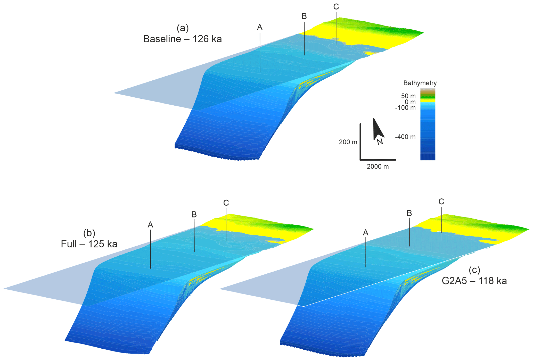
Figure 7Maximum inundation time step for each scenario. (a) Baseline model run with peak sea level at 2.11 m a.m.s.l. (b) Full scenario with peak sea level at 8.33 m a.m.s.l. (c) G2A5 scenario with peak sea level at 6.43 m a.m.s.l.
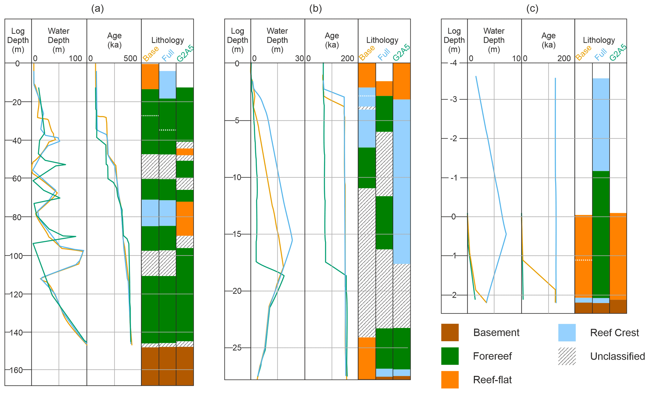
Figure 8Dionisos model well logs for (a) Well A, (b) Well B, and (c) Well C. Water depth is depth of original deposition, age is time of deposition, and the dotted white lines represent unconformities. Line color corresponds to scenario: orange = Base, blue = Full, and green = G2A5.
As described in Sect. 2.9, erosion and sediment transport within Dionisos is reliant on user-defined maximum values and simplified diffusion equations, respectively. While we do see preserved exposed fossil MIS 5e reef facies at Lembetabe (e.g., Battistini, 1965; Boyden et al., 2022), the corresponding MIS 5e sequences within produced synthetic well logs are sometimes lacking (Fig. 8c). This “preservation bias” is especially apparent when following the progression of sedimentation through the LIG. As pointed out in Sect. 3.1, under each scenario, multi-meter sections of lithology are removed in the intervening millennia between the LIG and modern (Fig. 9c–e). While each scenario deposits LIG reef facies at Well C, timing and amount vary significantly. For example, peak sedimentation under the Baseline is reached by 124 ka versus 122 ka under the Full scenario and 116 ka under G2A5. Of the three scenarios, the highest deposit in elevation is an intertidal facies under the Full scenario at 6.6 m a.m.s.l. (Fig. 9d). This is then followed by the G2A5 scenario at 116 ka with an intertidal facies at +4.9 m a.m.s.l. (Fig. 9e). However, of the three scenarios, only the Full scenario has preserved LIG reef facies above modern sea level (Fig. 8c). This is further reinforced by the exposure times under each scenario for Well B. Under all three scenarios, the area shoreward of the mid-platform is left exposed for +115 kyr before the final phase of Holocene sedimentation (Fig. 3). Such a long exposure time would, if maximum weathering rates were maintained, potentially lead to 11.5 m of erosion.
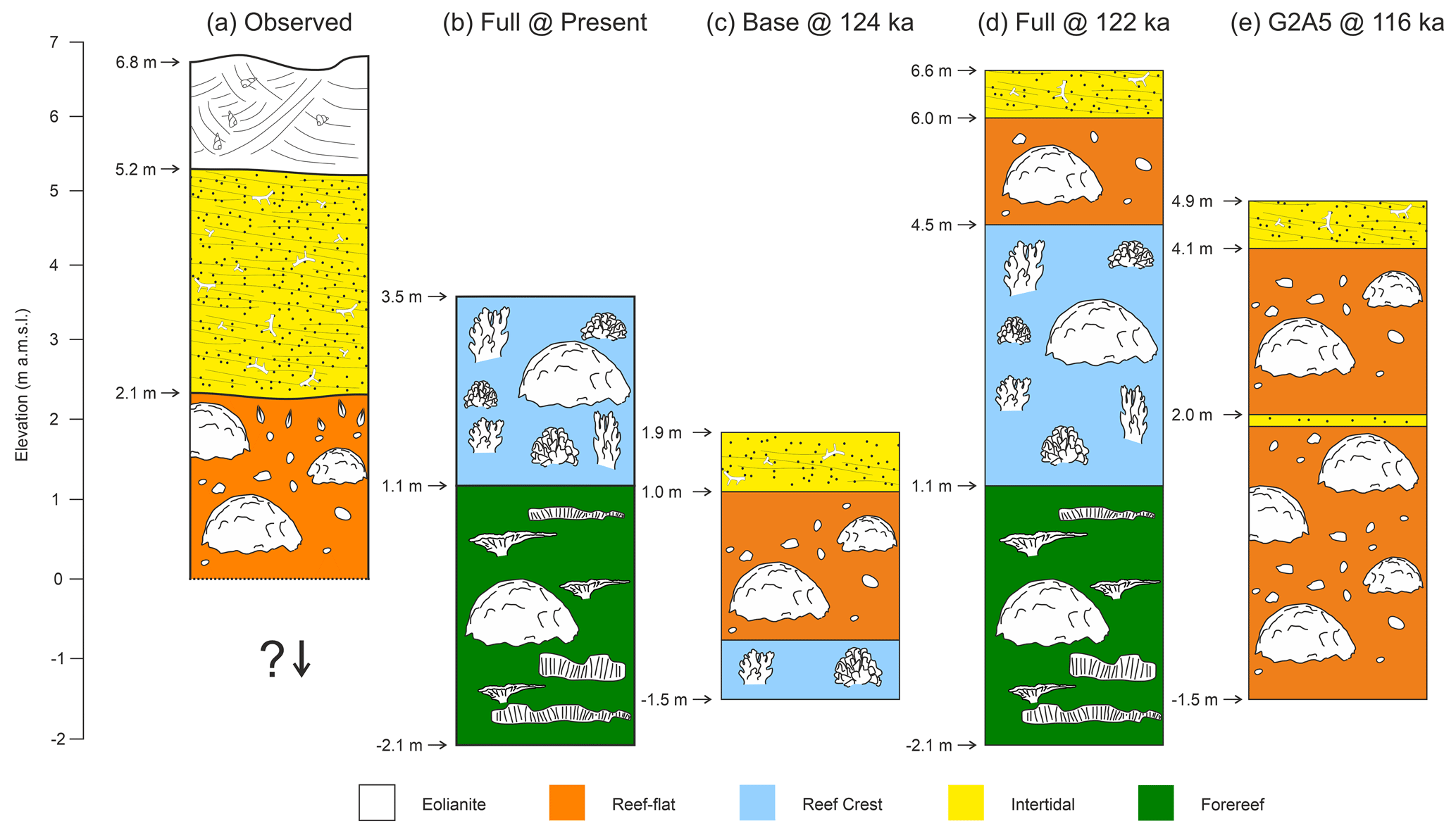
Figure 9Comparison between field observations made by Boyden et al. (2022), lithology extracted from Full scenario at Well C at the end of the model run, and the lithologies for the Base, Full, and G2A5 scenarios at their highest respective MIS 5e unit before erosion takes place. (a) Synthesized litholog based on mean maximum facies elevations reported in Boyden et al. (2022). According to Boyden et al. (2022), the reef flat correlates to the MIS 5e highstand, the intertidal facies represents the close of MIS 5e, and the eolianite closes out the sequence correlating to much younger deposition. (b) Lithology at Well C for Full scenario at end of simulation. (c) Lithology at Well C for Baseline scenario at 124 ka when regression begins. (d) Lithology at Well C for Full scenario at 122 ka. (e) Lithology at Well C for G2A5 scenario at 116 ka. Colors represent the declared lithologies within the model environment and major bioconstructors are included for cross-comparison purposes.
Unlike the previous investigations utilizing the Dionisos model elsewhere (e.g., Montaggioni et al., 2015), a one-to-one comparison between the model and the fossil record through the use of borehole and 2D seismic data is not possible. However, trends within the model output are roughly analogous to observations in the field. In particular, the presence of significant reef facies 3.5 m a.m.s.l. under the Full scenario at Well C is in good agreement with recent descriptions of the LIG facies present at Lembetabe (e.g., Fig. 9 and Boyden et al., 2022). Here, Boyden et al. (2022) describes a fossil reef flat that is exposed at +2.1 m a.m.s.l., which is then covered by a 3.1 m thick unit of intertidal calcarenite. Out of the three scenarios tested, only the Full scenario has preserved LIG reef facies above modern sea level (forereef and reef crest, Fig. 8) as well as the ability to reproduce the general geomorphology of the modern coastline and the modern fringing reef (Fig. 6). While Well C under the Full scenario represents a more distal facies as that found exposed at Lembetabe, these minor discrepancies in elevations of such facies are most likely derived from differences in spatial geometry of the antecedent (pre-LIG) coast, variable weathering rates during glacial times, as well as possible vertical land motion in the region. To this end, the preserved forereef and reef crest produced by the Full scenario provides an upper bound of RSL rise during the LIG. In fact, in both other scenarios, Baseline and G2A5, the oldest reef facies exposed above modern sea level is a reef flat deposited during the Holocene transgression (10 ka, Fig. 8c). This would imply that, all other model parameters equal, in order for the G2A5 scenario to produce a preserved LIG reef, either the GrIS and AIS melt contributions would need to increase or there would need to be a further reduction in erosion rates within the model. Both of these situations would be hard to justify as the eustatic component of RSL is already above the upper bound of Dyer et al. (2021) (6.6 and 5.3 m, respectively) and the marine and subaerial erosion components are already approaching the minimum of accepted weathering rates (e.g., Paulay and McEdward, 1990).
While the application of the model is spatially limited, these insights into the sensitivity of the LIG geological record provide a starting point for further analysis of other, more GIA and tectonically diverse LIG coral-dominated coastlines. Additional investigation into the interplay between GrIS and AIS contribution magnitude and timing is warranted. Furthermore, specific effort should be placed in testing locations where previous RSL curves similar in geometry to the G2A5 scenario explored here have been described.
In tropical and sub-tropical regions, field evidence-based constraints of LIG eustatic sea level often rely upon incomplete, temporally limited preservation of fossil coral reef facies. This, in turn, leaves the derivation of LIG sea level patterns up to interpretation and “expert judgment”. Here, we apply a suite of GIA models to a fringing reef system offshore southwestern Madagascar within the Dionisos forward stratigraphic model environment. The resulting stratigraphic sequences of two distinct GrIS and AIS melting scenarios during the LIG are then evaluated against the observed lithostratigraphy and a baseline pure GIA signal. By creating fictitious stratigraphic sequences based on physical principles, we are able to conclude that (1) changes in the timing of GrIS and AIS melting produce substantial visible changes in the stratigraphic record, (2) preservation within the coastal environment heavily influences the interpretation of the fossil reef and the derived paleo relative sea level, and (3) adoption of this methodology, while not a one-to-one comparison, would allow for a more objective evaluation of outcrop interpretation. We further conclude that based on these initial results, there is a compelling need for stability within the LIG, which is underlined by the lack of reef facies preserved under a two-peak sea level scenario. While significant sedimentation takes place during the LIG under a two-peak scenario, the intermittent sub-aerial exposure of the freshly deposited reef drastically decreases the robustness of the LIG record, bringing into question the possibility of observing such relative sea level fluctuations in the fossil record.
Forward stratigraphic model input files and GIA model outputs are available at https://doi.org/10.5281/zenodo.7565917 (Version 1.0, Boyden et al., 2023).
The supplement related to this article is available online at: https://doi.org/10.5194/esurf-11-917-2023-supplement.
PB, PS, and AR conceived the project; PS provided the GIA sea level scenario inputs; PB and AR evaluated model inputs; PB ran and analyzed model runs; PB wrote the initial manuscript; all authors reviewed and edited the article.
The contact author has declared that none of the authors has any competing interests.
Publisher’s note: Copernicus Publications remains neutral with regard to jurisdictional claims in published maps and institutional affiliations.
We would like to thank Beicip-Franlab for providing an academic license to OpenFlow Suite and Dionisos. Finally, we would like to thank Georgia Grant and Gino de Gelder for their constructive comments and reviews that helped improve the article.
This research was funded by the Deutsche Forschungsgemeinschaft Excellence Cluster “EXC 2077: The Ocean Floor – Earth’s Uncharted Interface” (grant no. 390741603) and the European Research Council under the European Union’s Horizon 2020 research and innovation program (grant no. 802414).
The article processing charges for this open-access publication were covered by the University of Bremen.
This paper was edited by Orencio Duran Vinent and reviewed by Gino de Gelder and Georgia Grant.
Austermann, J., Mitrovica, J. X., Huybers, P., and Rovere, A.: Detection of a dynamic topography signal in last interglacial sea-level records, Sci. Adv., 3, e1700457, https://doi.org/10.1126/sciadv.1700457, 2017. a
Barlow, N. L. M., McClymont, E. L., Whitehouse, P. L., Stokes, C. R., Jamieson, S. S. R., Woodroffe, S. A., Bentley, M. J., Callard, S. L., Cofaigh, C. Ó., Evans, D. J. A., Horrocks, J. R., Lloyd, J. M., Long, A. J., Margold, M., Roberts, D. H., and Sanchez-Montes, M. L.: Lack of evidence for a substantial sea-level fluctuation within the Last Interglacial, Nat. Geosci., 11, 627–634, 2018. a, b, c
Barrett, S. J. and Webster, J. M.: Holocene evolution of the Great Barrier Reef: Insights from 3D numerical modelling, Sediment. Geol., 265–266, 56–71, https://doi.org/10.1016/j.sedgeo.2012.03.015, 2012. a
Barrett, S. J. and Webster, J. M.: Reef Sedimentary Accretion Model (ReefSAM): Understanding coral reef evolution on Holocene time scales using 3D stratigraphic forward modelling, Mar. Geol., 391, 108–126, https://doi.org/10.1016/j.margeo.2017.07.007, 2017. a, b
Battistini, R.: Etude géomorphologique de l'Extrême-Sud de Madagascar, Ph.D. thesis, University of Madagascar, Toulouse, 1964. a
Battistini, R.: L'extrême-Sud de Madagascar, L'Information Géographique, 29, 83–84, 1965. a, b
BieicipFranlab: OpenFlow Suite, IFP Energies nouvelles, 2021. a
Bintanja, R. and van de Wal, R. S. W.: North American ice-sheet dynamics and the onset of 100,000-year glacial cycles, Nature, 454, 869–872, https://doi.org/10.1038/nature07158, 2008. a
Boyden, P., Weil-Accardo, J., Deschamps, P., Godeau, N., Jaosedy, N., Guihou, A., Rajaonarivelo, M. N., O’Leary, M., Humblet, M., and Rovere, A.: Revisiting Battistini: Pleistocene Coastal Evolution of Southwestern Madagascar, Open Quaternary, 8, 14, https://doi.org/10.5334/oq.112, 2022. a, b, c, d, e, f, g, h, i, j, k, l
Boyden, P., Stocchi, P., and Rovere, A.: Electronic Supplementary for: Refining patterns of melt with forward stratigraphic models on stable Pleistocene coastlines, Zenodo [data set], https://doi.org/10.5281/zenodo.7565917, 2023. a
Bristow, C., Lancaster, N., and Duller, G.: Combining ground penetrating radar surveys and optical dating to determine dune migration in Namibia, J. Geol. Soc. London, 162, 315–321, https://doi.org/10.1144/0016-764903-120, 2005. a
Burgess, P. M. and Pollitt, D. A.: The origins of shallow-water carbonate lithofacies thickness distributions: one-dimensional forward modelling of relative sea-level and production rate control, Sedimentology, 59, 57–80, https://doi.org/10.1111/j.1365-3091.2011.01303.x, 2012. a
Camoin, G. and Webster, J.: Coral reef response to Quaternary sea‐level and environmental changes: State of the science, Sedimentology, 62, 401–428, 2015. a, b
Côté-Laurin, M.-C., Benbow, S., and Erzini, K.: The short-term impacts of a cyclone on seagrass communities in Southwest Madagascar, Cont. Shelf Res., 138, 132–141, 2017. a
Creveling, J. R., Mitrovica, J. X., Hay, C. C., Austermann, J., and Kopp, R. E.: Revisiting tectonic corrections applied to Pleistocene sea-level highstands, Quaternary Sci. Rev., 111, 72–80, https://doi.org/10.1016/j.quascirev.2015.01.003, 2015. a
de Boer, B., van de Wal, R. S. W., Lourens, L. J., Bintanja, R., and Reerink, T. J.: A continuous simulation of global ice volume over the past 1 million years with 3-D ice-sheet models, Clim. Dynam., 41, 1365–1384, https://doi.org/10.1007/s00382-012-1562-2, 2013. a, b
de Boer, B., Stocchi, P., and van de Wal, R. S. W.: A fully coupled 3-D ice-sheet–sea-level model: algorithm and applications, Geosci. Model Dev., 7, 2141–2156, https://doi.org/10.5194/gmd-7-2141-2014, 2014. a
de Gelder, G., Jara-Muñoz, J., Melnick, D., Fernández-Blanco, D., Rouby, H., Pedoja, K., Husson, L., Armijo, R., and Lacassin, R.: How do sea-level curves influence modeled marine terrace sequences?, Quaternary Sci. Rev., 229, 106132, https://doi.org/10.1016/j.quascirev.2019.106132, 2020. a
DeConto, R. M. and Pollard, D.: Contribution of Antarctica to past and future sea-level rise, Nature, 531, 591–597, https://doi.org/10.1038/nature17145, 2016. a
Du Puy, D. and Moat, J.: A refined classification of the primary vegetation of Madagascar based on the underlying geology: using GIS to map its distribution and to assess its conservation status, Biogéographie de Madagascar, 1996, 205–218, 1996. a, b
Durrant, T., Hemer, M., Smith, G., Trenham, C., and Greenslade, D.: CAWCR Wave Hindcast-Aggregated Collection, http://hdl.handle.net/102.100.100/13165?index=1 (last access: 1 November 2021), 2013. a
Dutton, A., Webster, J. M., Zwartz, D., Lambeck, K., and Wohlfarth, B.: Tropical tales of polar ice: evidence of Last Interglacial polar ice sheet retreat recorded by fossil reefs of the granitic Seychelles islands, Quaternary Sci. Rev., 107, 182–196, https://doi.org/10.1016/j.quascirev.2014.10.025, 2015. a
Dyer, B., Austermann, J., D'Andrea, W. J., Creel, R. C., Sandstrom, M. R., Cashman, M., Rovere, A., and Raymo, M. E.: Sea-level trends across The Bahamas constrain peak last interglacial ice melt, P. Natl. Acad. Sci., 118, 33, https://doi.org/10.1073/pnas.2026839118, 2021. a, b, c
Edwards, T. L., Brandon, M. A., Durand, G., Edwards, N. R., Golledge, N. R., Holden, P. B., Nias, I. J., Payne, A. J., Ritz, C., and Wernecke, A.: Revisiting Antarctic ice loss due to marine ice-cliff instability, Nature, 566, 58–64, https://doi.org/10.1038/s41586-019-0901-4, 2019. a
Enos, P. and Franseen, E.: Sedimentary parameters for computer modeling, Sedimentary Modeling: Computer Simulations and Methods for Improved Parameter Definition: Kansas Geological Survey, Bulletin, 233, 63–99, 1991. a
Gardner, T. A., Côté, I. M., Gill, J. A., Grant, A., and Watkinson, A. R.: Hurricanes and Caribbean coral reefs: impacts, recovery patterns, and role in long‐term decline, Ecology, 86, 174–184, https://doi.org/10.1890/04-0141, 2005. a
Gischler, E., Hudson, J. H., Humblet, M., Braga, J. C., Schmitt, D., Isaack, A., Eisenhauer, A., and Camoin, G. F.: Holocene and Pleistocene fringing reef growth and the role of accommodation space and exposure to waves and currents (Bora Bora, Society Islands, French Polynesia), Sedimentology, 66, 305–328, https://doi.org/10.1111/sed.12533, 2019. a
Govin, A., Braconnot, P., Capron, E., Cortijo, E., Duplessy, J.-C., Jansen, E., Labeyrie, L., Landais, A., Marti, O., Michel, E., Mosquet, E., Risebrobakken, B., Swingedouw, D., and Waelbroeck, C.: Persistent influence of ice sheet melting on high northern latitude climate during the early Last Interglacial, Clim. Past, 8, 483–507, https://doi.org/10.5194/cp-8-483-2012, 2012. a
Granjeon, D., Joseph, P., Harbaugh, J. W., Watney, W. L., Rankey, E. C., Slingerland, R., Goldstein, R. H., and Franseen, E. K.: Concepts and Applications of A 3-D Multiple Lithology, Diffusive Model in Stratigraphic Modeling, Vol. 62, SEPM Society for Sedimentary Geology, https://doi.org/10.2110/pec.99.62.0197, 1999. a, b
Holthuijsen, L. H.: Waves in Oceanic and Coastal Waters, Cambridge University Press, Cambridge, https://doi.org/10.1017/CBO9780511618536, 2007. a
Kolodka, C., Vennin, E., Bourillot, R., Granjeon, D., and Desaubliaux, G.: Stratigraphic modelling of platform architecture and carbonate production: a Messinian case study (Sorbas Basin, SE Spain), Basin Res., 28, 658–684, https://doi.org/10.1111/bre.12125, 2016. a
Kopp, R. E., Simons, F. J., Mitrovica, J. X., Maloof, A. C., and Oppenheimer, M.: Probabilistic assessment of sea level during the last interglacial stage, Nature, 462, 863–867, https://doi.org/10.1038/nature08686, 2009. a
Lanteaume, C., Fournier, F., Pellerin, M., and Borgomano, J.: Testing geologic assumptions and scenarios in carbonate exploration: Insights from integrated stratigraphic, diagenetic, and seismic forward modeling, The Leading Edge, 37, 672–680, https://doi.org/10.1190/tle37090672.1, 2018. a
Lee, E. Y., Kominz, M., Reuning, L., Gallagher, S. J., Takayanagi, H., Ishiwa, T., Knierzinger, W., and Wagreich, M.: Quantitative compaction trends of Miocene to Holocene carbonates off the west coast of Australia, Aust. J. Earth Sci., 68, 1149–1161, https://doi.org/10.1080/08120099.2021.1915867, 2021. a
Malatesta, L. C., Finnegan, N. J., Huppert, K. L., and Carreño, E. I.: The influence of rock uplift rate on the formation and preservation of individual marine terraces during multiple sea-level stands, Geology, 50, 101–105, https://doi.org/10.1130/g49245.1, 2022. a, b
Montaggioni, L. F.: History of Indo-Pacific coral reef systems since the last glaciation: Development patterns and controlling factors, Earth-Sci. Rev., 71, 1–75, https://doi.org/10.1016/j.earscirev.2005.01.002, 2005. a, b
Montaggioni, L. F. and Braithwaite, C. J.: Quaternary coral reef systems: history, development processes and controlling factors, Elsevier, ISBN 9780080932767, 2009. a
Montaggioni, L. F. and Hoang, C.: The last interglacial high sea level in the granitic Seychelles, Indian Ocean, Palaeogeogr. Palaeocl., 64, 79–91, 1988. a
Montaggioni, L. F., Borgomano, J., Fournier, F., and Granjeon, D.: Quaternary atoll development: New insights from the two‐dimensional stratigraphic forward modelling of Mururoa Island (Central Pacific Ocean), Sedimentology, 62, 466–500, https://doi.org/10.1111/sed.12175, 2015. a, b, c, d, e, f, g, h
Noble, T., Rohling, E., Aitken, A. R. A., Bostock, H. C., Chase, Z., Gomez, N., Jong, L. M., King, M. A., Mackintosh, A. N., and McCormack, F.: The sensitivity of the Antarctic ice sheet to a changing climate: past, present, and future, Rev. Geophys., 58, e2019RG000663, https://doi.org/10.1029/2019RG000663, 2020. a
O’Leary, M. J., Hearty, P. J., Thompson, W. G., Raymo, M. E., Mitrovica, J. X., and Webster, J. M.: Ice sheet collapse following a prolonged period of stable sea level during the last interglacial, Nat. Geosci., 6, 796–800, https://doi.org/10.1038/ngeo1890, 2013. a, b, c
Pall, J., Chandra, R., Azam, D., Salles, T., Webster, J. M., Scalzo, R., and Cripps, S.: Bayesreef: A Bayesian inference framework for modelling reef growth in response to environmental change and biological dynamics, Environ. Modell. Softw., 125, 104610, https://doi.org/10.1016/j.envsoft.2019.104610, 2020. a
Paulay, G. and McEdward, L. R.: A simulation model of island reef morphology: the effects of sea level fluctuations, growth, subsidence and erosion, Coral Reefs, 9, 51–62, https://doi.org/10.1007/bf00368800, 1990. a, b
Revil, A., Grauls, D., and Brévart, O.: Mechanical compaction of sand/clay mixtures, J. Geophys. Res.-Sol. Ea., 107, 2293, https://doi.org/10.1029/2001JB000318, 2002. a
Roelvink, J., Reniers, A. J. H. M., van Dongeren, A. R., van Thiel de Vries, J. S. M., McCall, R. T., and Lescinski, J.: Modelling storm impacts on beaches, dunes and barrier islands, Coast. Eng., 56, 1133–1152, https://doi.org/10.1016/j.coastaleng.2009.08.006, 2009. a
Rovere, A., Raymo, M. E., Vacchi, M., Lorscheid, T., Stocchi, P., Gomez-Pujol, L., Harris, D. L., Casella, E., O'Leary, M. J., and Hearty, P. J.: The analysis of Last Interglacial (MIS 5e) relative sea-level indicators: Reconstructing sea-level in a warmer world, Earth-Sci. Rev., 159, 404–427, https://doi.org/10.1016/j.earscirev.2016.06.006, 2016. a
Salles, T., Pall, J., Webster, J. M., and Dechnik, B.: Exploring coral reef responses to millennial-scale climatic forcings: insights from the 1-D numerical tool pyReef-Core v1.0, Geosci. Model Dev., 11, 2093–2110, https://doi.org/10.5194/gmd-11-2093-2018, 2018. a
Seard, C., Borgomano, J., Granjeon, D., and Camoin, G.: Impact of environmental parameters on coral reef development and drowning: Forward modelling of the last deglacial reefs from Tahiti (French Polynesia; IODP Expedition #310), Sedimentology, 60, 1357–1388, 2013. a, b, c, d, e
Simms, A. R., Anderson, J. B., DeWitt, R., Lambeck, K., and Purcell, A.: Quantifying rates of coastal subsidence since the last interglacial and the role of sediment loading, Global Planet. Change, 111, 296–308, https://doi.org/10.1016/j.gloplacha.2013.10.002, 2013. a
Spada, G. and Stocchi, P.: SELEN: A Fortran 90 program for solving the “sea-level equation”, Comput. Geosci., 33, 538–562, https://doi.org/10.1016/j.cageo.2006.08.006, 2007. a
Stone, E. J., Capron, E., Lunt, D. J., Payne, A. J., Singarayer, J. S., Valdes, P. J., and Wolff, E. W.: Impact of meltwater on high-latitude early Last Interglacial climate, Clim. Past, 12, 1919–1932, https://doi.org/10.5194/cp-12-1919-2016, 2016. a
Tierney, J. E., Poulsen, C. J., Montañez, I. P., Bhattacharya, T., Feng, R., Ford, H. L., Hönisch, B., Inglis, G. N., Petersen, S. V., Sagoo, N., Tabor, C. R., Thirumalai, K., Zhu, J., Burls, N. J., Foster, G. L., Goddéris, Y., Huber, B. T., Ivany, L. C., Kirtland Turner, S., Lunt, D. J., McElwain, J. C., Mills, B. J. W., Otto-Bliesner, B. L., Ridgwell, A., and Zhang, Y. G.: Past climates inform our future, Science, 370, 6517, https://doi.org/10.1126/science.aay3701, 2020. a
Trudgill, S. T., Stoddart, D. R., and Westoll, T. S.: Surface lowering and landform evolution on Aldabra, Philosophical Transactions of the Royal Society of London. B, Biological Sciences, 286, 35–45, https://doi.org/10.1098/rstb.1979.0014, 1979. a, b
Vyverberg, K., Dechnik, B., Dutton, A., Webster, J. M., Zwartz, D., and Portell, R. W.: Episodic reef growth in the granitic Seychelles during the Last Interglacial: implications for polar ice sheet dynamics, Mar. Geol., 399, 170–187, https://doi.org/10.1016/j.margeo.2018.02.010, 2018. a
Warrlich, G., Waltham, D., and Bosence, D.: Quantifying the sequence stratigraphy and drowning mechanisms of atolls using a new 3‐D forward stratigraphic modelling program (CARBONATE 3D), Basin Res., 14, 379–400, https://doi.org/10.1046/j.1365-2117.2002.00181.x, 2002. a
Warrlich, G., Bosence, D., Waltham, D., Wood, C., Boylan, A., and Badenas, B.: 3D stratigraphic forward modelling for analysis and prediction of carbonate platform stratigraphies in exploration and production, Mar. Petrol. Geol., 25, 35–58, https://doi.org/10.1016/j.marpetgeo.2007.04.005, 2008. a
Weil-Accardo, J., Boyden, P., Rovere, A., Godeau, N., Jaosedy, N., Guihou, A., Humblet, M., Rajaonarivelo, M., Austermann, J., and Deschamps, P.: New datings and elevations of a fossil reef in Lembetabe, southwest Madagascar: eustatic and tectonic implications, Quaternary Sci. Rev., 313, 108197, https://doi.org/10.1016/j.quascirev.2023.108197, 2023. a
Woodroffe, C. D.: Coasts: Form, Process and Evolution, Cambridge University Press, Cambridge, https://doi.org/10.1017/CBO9781316036518, 2002. a
Woodroffe, C. D. and Webster, J. M.: Coral reefs and sea-level change, Mar. Geol., 352, 248–267, https://doi.org/10.1016/j.margeo.2013.12.006, 2014. a