Linear-stability analysis of plane beds under flows with suspended loads

Plane beds develop under flows in fluvial and marine environments; they are recorded as parallel lamination in sandstone beds, such as those found in turbidites. However, whereas turbidites typically exhibit parallel lamination, they rarely feature dune-scale cross-lamination. Although the reason for the scarcity of dune-scale cross-lamination in turbidites is still debated, the formation of dunes may be dampened by suspended loads. Here, we perform, for the first time, linear-stability analysis to show that flows with suspended loads facilitate the formation of plane beds. For a fine-grained bed, a suspended load can promote the formation of plane beds and dampen the formation of dunes. These results of theoretical analysis were verified with observational data of plane beds under open-channel flows. Our theoretical analysis found that suspended loads promote the formation of plane beds, which suggests that the development of dunes under turbidity currents is suppressed by the presence of suspended loads.

1 Introduction

The interactions between fluids and erodible surfaces generate small-scale topographic features called bedforms on both terrestrial surfaces (e.g., riverbeds, deserts, and deep-sea floors) and extra-terrestrial surfaces (Bourke et al., 2010; Gao et al., 2015; Hage et al., 2018; Cisneros et al., 2020). Such bedforms are preserved in sedimentary rocks as sedimentary structures such as cross-lamination and parallel lamination (Harms, 1979). The types of sedimentary structures observed vary among different types of rocks. Turbidites typically exhibit parallel lamination (Bouma, 1962), whereas they rarely feature dune-scale cross-lamination (Talling et al., 2012). However, the opposite is true for fluvial deposits; i.e., dune-scale cross-laminae are often observed in riverine sandstone (Miall, 2010).

Although the reason for the paucity of dune-scale cross-lamination in turbidites is still debated (Lowe, 1988; Arnott, 2012; Schindler et al., 2015; Tilston et al., 2015), it could be attributed to the presence of suspended loads. For example, in the case of open-channel flows, nearly flat-bed waves and low-angle dunes have been observed in suspension-dominated rivers (Smith and McLean, 1977; Kostaschuk and Villard, 1996; Bradley et al., 2013; Ma et al., 2017). Additionally, flume experiments have suggested that dune height decreases with increasing suspended-load flux (Bridge and Best, 1988; Naqshband et al., 2017). Therefore, the influence of suspended loads on the suppression of dune development and the formation of plane beds is worth investigating.

The relationships between sediment transport modes and the formation of plane beds have received little attention in theoretical works that performed linear-stability analyses. The reason could be that previous studies have succeeded in predicting the wavelength of dunes and antidunes without considering suspended loads (Colombini, 2004; Di Cristo et al., 2006; Colombini and Stocchino, 2008; Vesipa et al., 2012; Bohorquez et al., 2019). However, this assumption is not appropriate for analyzing open-channel flows where the suspended load is not negligible, such as flows in rivers with a fine sediment bed (de Almeida et al., 2016; Sambrook Smith et al., 2016). Moreover, although some research has considered both bed and suspended loads (Engelund, 1970; Nakasato and Izumi, 2008; Bose and Dey, 2009), the hydraulic conditions of these analyses were limited, and the results were tested using only observational data of dunes and antidunes.

Therefore, in order to investigate the effect of sediment transport mode on the formation of plane beds, we performed a linear-stability analysis of bedforms under open-channel flows carrying suspended loads. The model introduced in Nakasato and Izumi (2008) was extended in this study to evaluate plane bed formation under various conditions of sediment diameter and flow depth. To evaluate the suspended-load effect, linear-stability analyses were performed on flows both with and without suspended loads. Further, we tested our stability diagrams against observational data of plane beds. Our theoretical analysis reveals for the first time that suspended loads promote the formation of plane beds, which has implications for interpreting sedimentary structures in turbidites.

2 Methods

Linear-stability analysis of fluvial bedforms can provide the wavelengths of perturbations (i.e., bed waves) that grow over time (Colombini, 2004; Bohorquez et al., 2019). We employ the two-dimensional Reynolds-averaged Navier–Stokes equations as the governing equations for flows and the quasi-steady assumption to neglect the unsteady terms in the flow equations. The eddy viscosity is evaluated using a mixing-length approach. In this study, bed-load discharge is estimated using the Meyer-Peter and Müller formula modified as described in Wong and Parker (2006). The entrainment rate of the suspended load is estimated using the relationship proposed in de Leeuw et al. (2020). See the following section for details. To test the results of linear-stability analyses against the observational data of plane beds, we plotted stability diagrams in the parametric space of hydraulic parameters.

2.1 Governing parameters

The instability of a system is illustrated as a contour diagram of the perturbation growth rate ω_i (Fig. 1). Generally, theoretical studies of bedforms based on linear-stability analyses describe the transition of bedform phases in the parametric space of wavenumber k and Froude number Fr, which are given by

$$\begin{array}{}\text{(1)}& {\displaystyle }k={\displaystyle \frac{\mathrm{2}\mathit{\pi }{\stackrel{\mathrm{̃}}{h}}_{\mathrm{0}}}{\stackrel{\mathrm{̃}}{\mathit{\lambda }}}}\text{(2)}& {\displaystyle }\mathit{Fr}={\displaystyle \frac{{\stackrel{\mathrm{̃}}{U}}_{\mathrm{0}}}{\sqrt{\stackrel{\mathrm{̃}}{g}{\stackrel{\mathrm{̃}}{h}}_{\mathrm{0}}}}},\end{array}$$

where $\stackrel{\mathrm{̃}}{\mathit{\lambda }}$ denotes the perturbation wavelength, ${\stackrel{\mathrm{̃}}{U}}_{\mathrm{0}}$ is the depth-averaged flow velocity of the uniform flow, $\stackrel{\mathrm{̃}}{g}$ is the gravitational acceleration (i.e., 9.81 m² s⁻¹), and ${\stackrel{\mathrm{̃}}{h}}_{\mathrm{0}}$ is the flow depth of the uniform flow. Hereafter, we denote dimensional variables using a tilde.

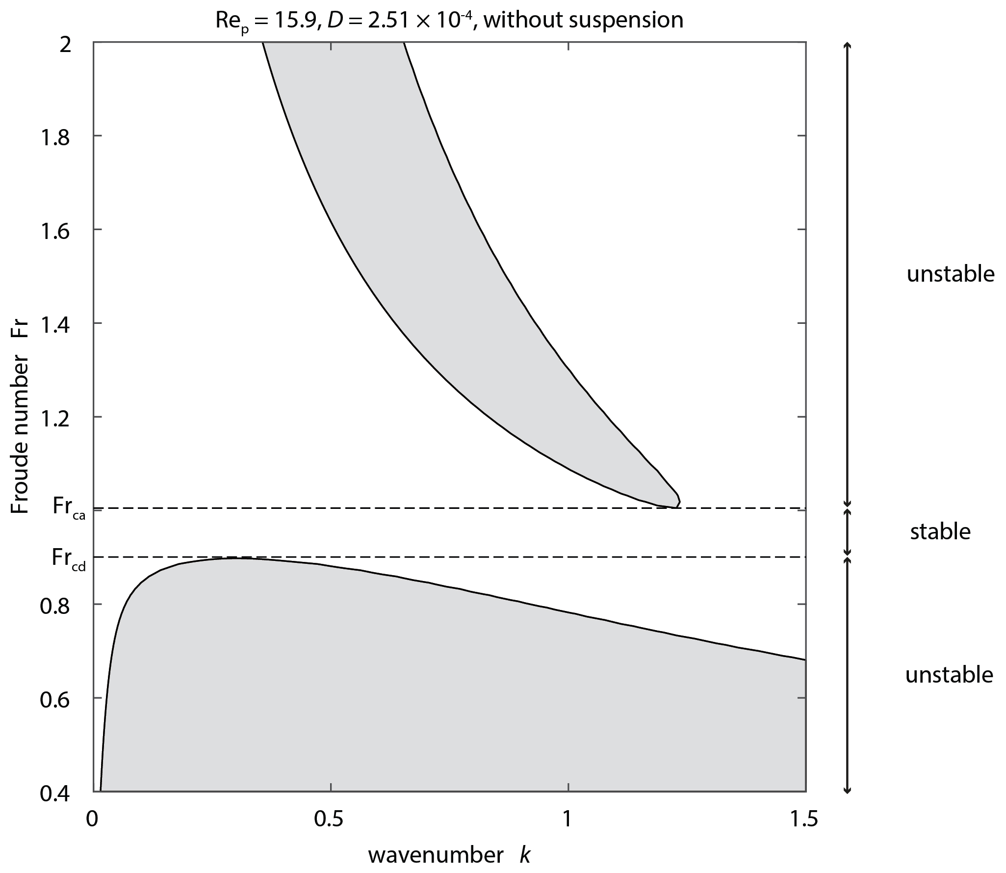
Figure 1 Contour map of perturbation growth rate ω_i without suspension. The particle Reynolds number and dimensionless particle diameter were set to Re_p=15.9 and $D=\mathrm{2.51}\times {\mathrm{10}}^{-\mathrm{4}}$, respectively. The dotted line denotes the threshold of sediment motion. The dashed lines denote the critical Froude numbers Fr_cd and Fr_ca for instabilities. The region where the growth rate is positive is highlighted in gray.

Stability diagrams described on the k–Fr plane have been commonly used to predict the development of dunes and antidunes (Kennedy, 1963). A few studies have used other combinations of dimensionless numbers such as the friction coefficient C versus Fr (Colombini and Stocchino, 2008) and the relative roughness $\stackrel{\mathrm{̃}}{D}/{\stackrel{\mathrm{̃}}{h}}_{\mathrm{0}}$ on the k–Fr plane (Bohorquez et al., 2019).

Although the classic k–Fr diagrams are widely accepted, we cannot use this approach to evaluate whether plane bed formation can be predicted reliably because plane beds have extremely small wavenumbers or have an infinite wavelength (i.e., they are flat). Therefore, we illustrate stability diagrams as contour maps of the maximum growth rate ω_i,max of the instability on the Re_p–Fr plane with fixed D and on the D–Fr plane with fixed Re_p to investigate the impact of suspended loads on the formation of plane beds. Here, D denotes the dimensionless particle diameter $\stackrel{\mathrm{̃}}{D}/{\stackrel{\mathrm{̃}}{h}}_{\mathrm{0}}$.

The instability of a system is illustrated as a contour diagram of the perturbation growth rate ω_i (Fig. 1). We can rewrite Eq. (A30) as

$$\begin{array}{}\text{(3)}& \mathit{\omega }=\mathit{\omega }\left(k,Fr,\stackrel{\mathrm{̃}}{D},{\stackrel{\mathrm{̃}}{h}}_{\mathrm{0}}\right).\end{array}$$

Thus, we can obtain the growth rate ω_i as a function of k for a given combination of Fr, $\stackrel{\mathrm{̃}}{D}$, and ${\stackrel{\mathrm{̃}}{h}}_{\mathrm{0}}$ (Figs. A3 and A4; Tables A1–A5). In this study, we assume that the system is stable if ω_i is not positive for all k within the domain [k_min, k_max] for a given Fr, $\stackrel{\mathrm{̃}}{D}$, and ${\stackrel{\mathrm{̃}}{h}}_{\mathrm{0}}$ combination. In contrast, the system is assumed to be unstable if ω_i is positive for some k (Fig. 1). We describe stability diagrams as contour maps of the maximum growth rate of the instability in the parametric space of (Re_p,Fr) (Fig. 2) and (D,Fr) (Fig. 3).

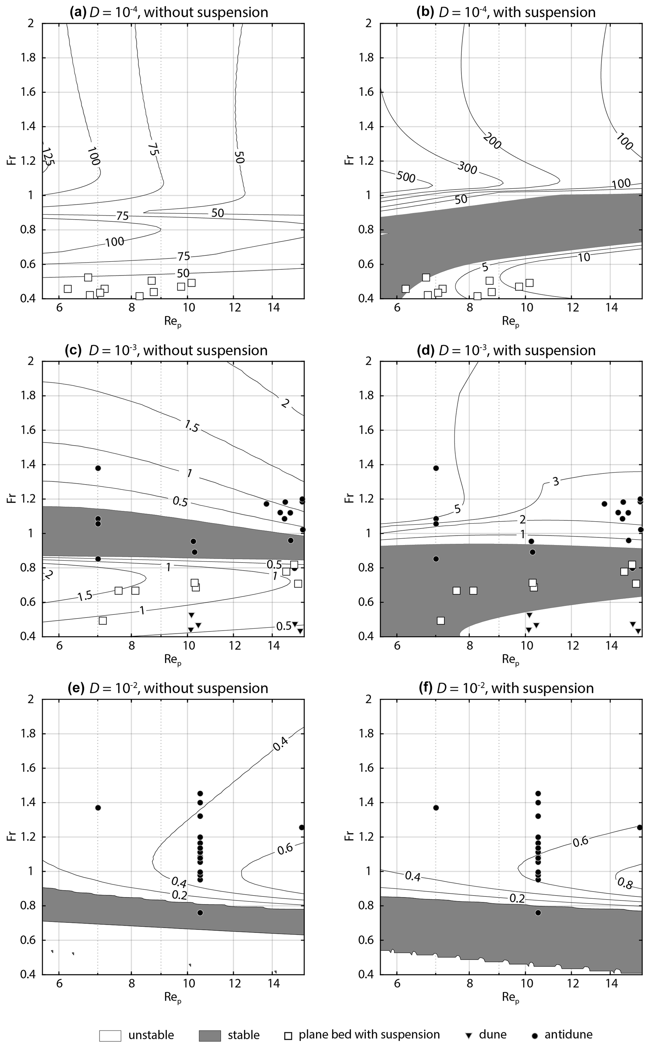
Figure 2 Contour maps of the maximum growth rate ω_i,max of perturbations with a fixed dimensionless particle diameter D. Symbols are observational data. (a) $D={\mathrm{10}}^{-\mathrm{4}}$ without suspension. (b) $D={\mathrm{10}}^{-\mathrm{4}}$ with suspension. (c) $D={\mathrm{10}}^{-\mathrm{3}}$ without suspension. (d) $D={\mathrm{10}}^{-\mathrm{3}}$ with suspension. (e) $D={\mathrm{10}}^{-\mathrm{2}}$ without suspension. (f) $D={\mathrm{10}}^{-\mathrm{2}}$ with suspension. (a, b) The range of D of observational data is from $\mathrm{3.16}\times {\mathrm{10}}^{-\mathrm{5}}$ to $\mathrm{3.16}\times {\mathrm{10}}^{-\mathrm{4}}$. (c, d) The range of D of observational data is from $\mathrm{3.16}\times {\mathrm{10}}^{-\mathrm{4}}$ to $\mathrm{3.16}\times {\mathrm{10}}^{-\mathrm{3}}$. (e, f) The range of D of observational data is from $\mathrm{3.16}\times {\mathrm{10}}^{-\mathrm{3}}$ to $\mathrm{3.16}\times {\mathrm{10}}^{-\mathrm{2}}$.

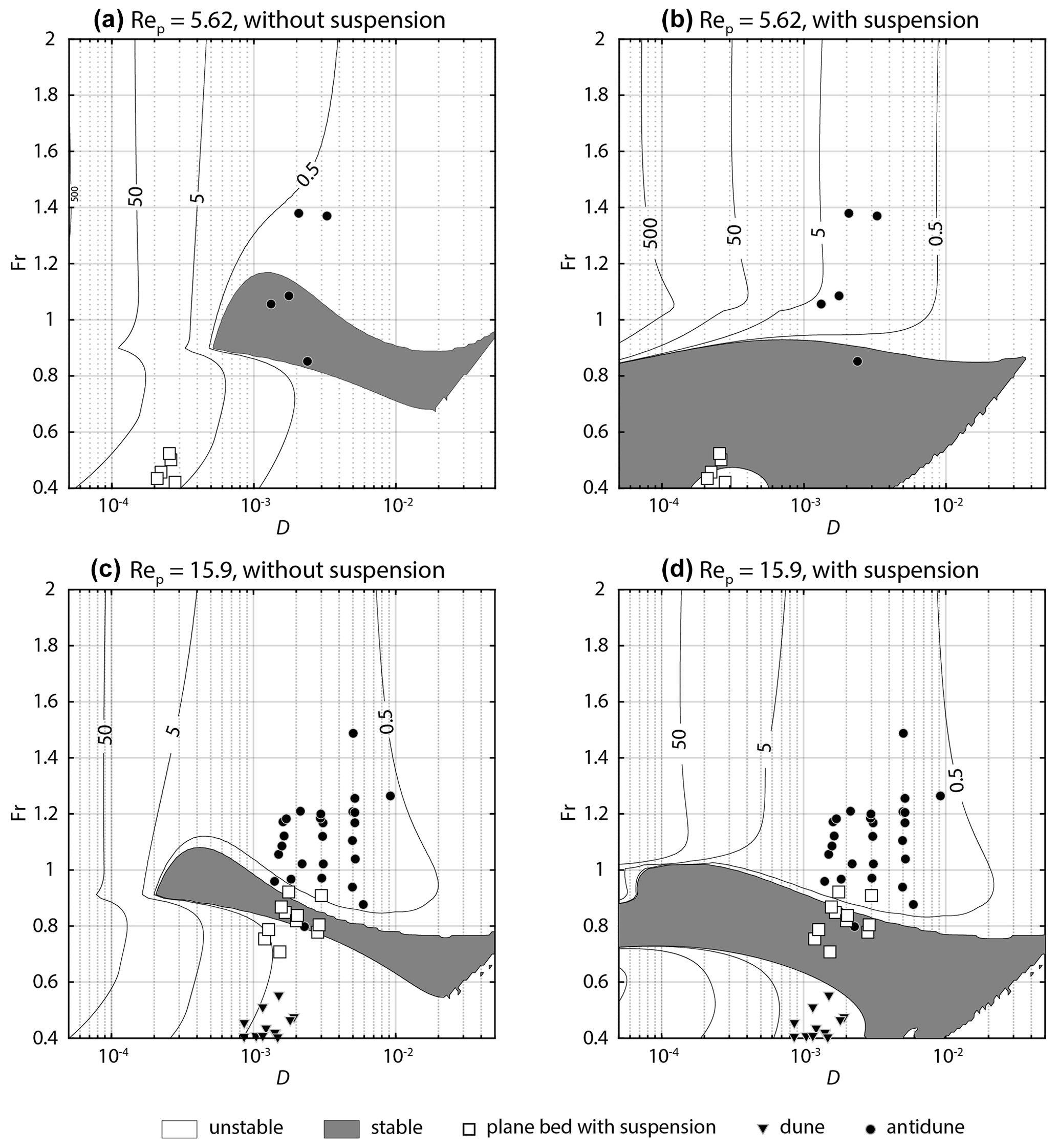
Figure 3 Contour maps of the maximum growth rate ω_i,max of perturbations with a fixed particle Reynolds number Re_p. Symbols are observational data. (a) Re_p=5.62 without suspension. (b) Re_p=5.62 with suspension. (c) Re_p=15.9 without suspension. (d) Re_p=15.9 with suspension. (a, b) The range of Re_p of observational data is from 4.46 to 7.0749. (c, d) The range of Re_p of observational data is from 12.6 to 20.

The domain [k_min,k_max] was set as [0.01,1.5], corresponding to λ ranging from ∼4.2h to ∼628h. The Froude number range was set as 0.4–2. For the Re_p–Fr diagram (Fig. 2), we employed three grades of D: $D={\mathrm{10}}^{-\mathrm{4}},{\mathrm{10}}^{-\mathrm{3}}$, and 10⁻². The particle Reynolds number Re_p ranges from 5.62 to 15.9 ($\stackrel{\mathrm{̃}}{D}=$ 0.125–0.25 mm). For the D–Fr diagram, we employed Re_p=5.62 and 15.9 as the fixed value of particle diameter. The dimensionless particle diameter D ranges from $\mathrm{5.0}\times {\mathrm{10}}^{-\mathrm{2}}$ to $\mathrm{5.0}\times {\mathrm{10}}^{-\mathrm{5}}$ in the D–Fr diagram (Fig. 3).

2.2 Linear-stability analysis

Here we present the formulation of the problem and the method used to solve the differential equations.

2.2.1 Flow equations

The governing equations for flows are the two-dimensional Reynolds-averaged Navier–Stokes equations. On erodible beds, the flow adjustments occur immediately relative to the bed adjustments (Fourrière et al., 2010). Therefore, we employ the quasi-steady assumption to neglect the unsteady terms in the flow equations (Colombini, 2004; Yokokawa et al., 2016).

Under the quasi-steady assumption, the dimensionless forms of the Reynolds-averaged Navier–Stokes equations and continuity equation for incompressible flow are described as

$$\begin{array}{}\text{(4)}& {\displaystyle }u{\displaystyle \frac{\partial u}{\partial x}}+w{\displaystyle \frac{\partial u}{\partial z}}=-{\displaystyle \frac{\partial p}{\partial x}}+\mathrm{1}+{\displaystyle \frac{\partial T_{xx}}{\partial x}}+{\displaystyle \frac{\partial T_{xz}}{\partial z}}\text{(5)}& {\displaystyle }u{\displaystyle \frac{\partial w}{\partial x}}+w{\displaystyle \frac{\partial w}{\partial z}}=-{\displaystyle \frac{\partial p}{\partial z}}+S^{-\mathrm{1}}+{\displaystyle \frac{\partial T_{xz}}{\partial x}}+{\displaystyle \frac{\partial T_{zz}}{\partial z}}\text{(6)}& {\displaystyle \frac{\partial u}{\partial x}}+{\displaystyle \frac{\partial w}{\partial z}}=\mathrm{0},\end{array}$$

where u and w are the flow velocities in the x and z directions, respectively; p denotes the pressure; S is the bed slope; and $T_{ij}(i,j=x,z)$ is the Reynolds stress tensor.

We employ a Boussinesq-type assumption to close the flow equations:

$$\begin{array}{}\text{(7)}& {\displaystyle }{T}_{xx}=\mathrm{2}{\mathit{\nu }}_T{\displaystyle \frac{\partial u}{\partial x}}\text{(8)}& {\displaystyle }{T}_{zz}=\mathrm{2}{\mathit{\nu }}_T{\displaystyle \frac{\partial w}{\partial z}}\text{(9)}& {\displaystyle }{T}_{xz}={\mathit{\nu }}_T\left({\displaystyle \frac{\partial u}{\partial x}}+{\displaystyle \frac{\partial w}{\partial z}}\right).\end{array}$$

Then, the eddy viscosity ν_T is evaluated using a mixing-length approach:

$$\begin{array}{}\text{(10)}& {\displaystyle }{\mathit{\nu }}_T=l^{\mathrm{2}}\left|{\displaystyle \frac{\partial u}{\partial z}}\right|\text{(11)}& {\displaystyle }l=\mathit{\kappa }(z-Z)\sqrt{{\displaystyle \frac{h+R-z}{h}}},\end{array}$$

where l is the mixing length, κ is the Kármán coefficient (i.e., 0.4), h is the flow depth, Z denotes the bed height, and R is the height of the reference level at which the flow velocity is assumed to vanish in a logarithmic profile (Fig. A1).

In the above equations, the system is non-dimensionalized as follows:

$$\begin{array}{}\text{(12)}& {\displaystyle }(u,w)=(\stackrel{\mathrm{̃}}{u},\stackrel{\mathrm{̃}}{w})/{\stackrel{\mathrm{̃}}{u}}_{{\mathrm{f}}_{\mathrm{0}}}\text{(13)}& {\displaystyle }(x,z,h,Z,R,D)=(\stackrel{\mathrm{̃}}{x},\stackrel{\mathrm{̃}}{z},\stackrel{\mathrm{̃}}{h},\stackrel{\mathrm{̃}}{Z},\stackrel{\mathrm{̃}}{R},\stackrel{\mathrm{̃}}{D})/{\stackrel{\mathrm{̃}}{h}}_{\mathrm{0}}\text{(14)}& {\displaystyle }(p,T_{ij})=(\stackrel{\mathrm{̃}}{p},{\stackrel{\mathrm{̃}}{T}}_{ij})/\stackrel{\mathrm{̃}}{\mathit{\rho }}{\stackrel{\mathrm{̃}}{h}}_{\mathrm{0}}\text{(15)}& {\displaystyle }{\mathit{\nu }}_T={\stackrel{\mathrm{̃}}{\stackrel{\mathrm{̃}}{\mathit{\nu }}}}_T/\left({\stackrel{\mathrm{̃}}{u}}_{{\mathrm{f}}_{\mathrm{0}}}{\stackrel{\mathrm{̃}}{h}}_{\mathrm{0}}\right),\end{array}$$

where D is the non-dimensional diameter of a bed particle, ${\stackrel{\mathrm{̃}}{u}}_{{\mathrm{f}}_{\mathrm{0}}}$ denotes the shear velocity in the basic flat-bed state, and $\stackrel{\mathrm{̃}}{\mathit{\rho }}$ is the water density (i.e., 1000 kg m³). The shear velocity in the basic flat-bed state ${\stackrel{\mathrm{̃}}{u}}_{{\mathrm{f}}_{\mathrm{0}}}$ is obtained as

$$\begin{array}{}\text{(16)}& {\stackrel{\mathrm{̃}}{u}}_{{\mathrm{f}}_{\mathrm{0}}}=\sqrt{\stackrel{\mathrm{̃}}{g}{\stackrel{\mathrm{̃}}{h}}_{\mathrm{0}}S}.\end{array}$$

As the flow is continuous, the system can be rewritten using the stream function ψ defined as

$$\begin{array}{}\text{(17)}& (u,w)=\left({\displaystyle \frac{\partial \mathit{\psi }}{\partial z}},-{\displaystyle \frac{\partial \mathit{\psi }}{\partial x}}\right).\end{array}$$

Then, Eqs. (4) and (5) are rearranged to

$$\begin{array}{}\text{(18)}& {\displaystyle }\begin{array}{rl}{\displaystyle \frac{\partial \mathit{\psi }}{\partial z}}{\displaystyle \frac{{\partial }^{\mathrm{2}}\mathit{\psi }}{\partial x\partial z}}-{\displaystyle \frac{\partial \mathit{\psi }}{\partial x}}{\displaystyle \frac{{\partial }^{\mathrm{2}}\mathit{\psi }}{\partial z^{\mathrm{2}}}}=& -{\displaystyle \frac{\partial p}{\partial x}}+\mathrm{1}+{\displaystyle \frac{\partial }{\partial x}}\left(\mathrm{2}{\mathit{\nu }}_T{\displaystyle \frac{{\partial }^{\mathrm{2}}\mathit{\psi }}{\partial x\partial z}}\right)\\ & +{\displaystyle \frac{\partial }{\partial z}}\left[{\mathit{\nu }}_T\left({\displaystyle \frac{{\partial }^{\mathrm{2}}\mathit{\psi }}{\partial z^{\mathrm{2}}}}-{\displaystyle \frac{{\partial }^{\mathrm{2}}\mathit{\psi }}{\partial x^{\mathrm{2}}}}\right)\right]\end{array}\text{(19)}& {\displaystyle }\begin{array}{rl}{\displaystyle \frac{\partial \mathit{\psi }}{\partial x}}{\displaystyle \frac{{\partial }^{\mathrm{2}}\mathit{\psi }}{\partial x\partial z}}-{\displaystyle \frac{\partial \mathit{\psi }}{\partial z}}{\displaystyle \frac{{\partial }^{\mathrm{2}}\mathit{\psi }}{\partial x^{\mathrm{2}}}}=& -{\displaystyle \frac{\partial p}{\partial z}}+S^{-\mathrm{1}}-{\displaystyle \frac{\partial }{\partial z}}\left(\mathrm{2}{\mathit{\nu }}_T{\displaystyle \frac{{\partial }^{\mathrm{2}}\mathit{\psi }}{\partial x\partial z}}\right)\\ & +{\displaystyle \frac{\partial }{\partial x}}\left[{\mathit{\nu }}_T\left({\displaystyle \frac{{\partial }^{\mathrm{2}}\mathit{\psi }}{\partial z^{\mathrm{2}}}}-{\displaystyle \frac{{\partial }^{\mathrm{2}}\mathit{\psi }}{\partial x^{\mathrm{2}}}}\right)\right]\end{array}.\end{array}$$

Eliminating p from Eqs. (18) and (19), we obtain

$$\begin{array}{}\text{(20)}& {\displaystyle }\begin{array}{rl}{\displaystyle \frac{\partial \mathit{\psi }}{\partial z}}{\displaystyle \frac{\partial }{\partial x}}{\mathrm{\nabla }}^{\mathrm{2}}\mathit{\psi }& -{\displaystyle \frac{\partial \mathit{\psi }}{\partial x}}{\displaystyle \frac{\partial }{\partial z}}{\mathrm{\nabla }}^{\mathrm{2}}\mathit{\psi }-\mathrm{4}{\displaystyle \frac{{\partial }^{\mathrm{2}}}{\partial x\partial z}}\left({\mathit{\nu }}_T{\displaystyle \frac{{\partial }^{\mathrm{2}}\mathit{\psi }}{\partial x\partial z}}\right)\\ & +\left({\displaystyle \frac{{\partial }^{\mathrm{2}}}{\partial x^{\mathrm{2}}}}-{\displaystyle \frac{{\partial }^{\mathrm{2}}}{\partial z^{\mathrm{2}}}}\right)\left[{\mathit{\nu }}_T\left({\displaystyle \frac{{\partial }^{\mathrm{2}}}{\partial z^{\mathrm{2}}}}-{\displaystyle \frac{{\partial }^{\mathrm{2}}}{\partial x^{\mathrm{2}}}}\right)\mathit{\psi }\right]=\mathrm{0}\end{array}.\end{array}$$

2.2.2 Advection–diffusion equations for suspended sediment

We also assume a quasi-steady state for the advection–diffusion equation for suspended sediment, which is formulated as

$$\begin{array}{}\text{(21)}& {\displaystyle \frac{\partial F_x}{\partial x}}+{\displaystyle \frac{\partial F_z}{\partial z}}=\mathrm{0}.\end{array}$$

Here, F_x and F_z are the normalized fluxes of suspended sediment in the x and z directions, respectively, given by

$$\begin{array}{}\text{(22)}& {\displaystyle }{F}_x=uc-{\mathit{\nu }}_T{\displaystyle \frac{\partial c}{\partial x}}\text{(23)}& {\displaystyle }{F}_z=(w-w_{\mathrm{s}})c-{\mathit{\nu }}_T{\displaystyle \frac{\partial c}{\partial z}},\end{array}$$

where c denotes the concentration of suspended sediment, and w_s is the settling velocity of sediment. We assume that the diffusion coefficient of suspended sediment is equal to the eddy viscosity ν_T. Based on Eqs. (22) and (23), Eq. (21) is reformulated as

$$\begin{array}{}\text{(24)}& u{\displaystyle \frac{\partial c}{\partial x}}+(w-w_{\mathrm{s}}){\displaystyle \frac{\partial c}{\partial z}}={\displaystyle \frac{\partial }{\partial x}}\left({\mathit{\nu }}_T{\displaystyle \frac{\partial c}{\partial x}}\right)+{\displaystyle \frac{\partial }{\partial z}}\left({\mathit{\nu }}_T{\displaystyle \frac{\partial c}{\partial z}}\right).\end{array}$$

The settling velocity of sediment w_s is calculated using a relationship given in Ferguson and Church (2004):

$$\begin{array}{}\text{(25)}& {\displaystyle }{w}_{\mathrm{s}}={\displaystyle \frac{{\stackrel{\mathrm{̃}}{w}}_{\mathrm{s}}}{\sqrt{R_{\mathrm{s}}\stackrel{\mathrm{̃}}{g}\stackrel{\mathrm{̃}}{D}}}}\text{(26)}& {\displaystyle }{\stackrel{\mathrm{̃}}{w}}_{\mathrm{s}}={\displaystyle \frac{R_{\mathrm{s}}\stackrel{\mathrm{̃}}{g}{\stackrel{\mathrm{̃}}{D}}^{\mathrm{2}}}{C_{\mathrm{1}}\stackrel{\mathrm{̃}}{\mathit{\nu }}+\mathrm{0.75}{C}_{\mathrm{2}}\sqrt{R_{\mathrm{s}}\stackrel{\mathrm{̃}}{g}{\stackrel{\mathrm{̃}}{D}}^{\mathrm{3}}}}},\end{array}$$

where the constants C₁ and C₂ are set to the values for natural sand (C₁=18 and C₂=1.0).

The particle Reynolds number Re_p is defined as

$$\begin{array}{}\text{(27)}& R{e}_{\mathrm{p}}={\displaystyle \frac{\sqrt{R_{\mathrm{s}}\stackrel{\mathrm{̃}}{g}{\stackrel{\mathrm{̃}}{D}}^{\mathrm{3}}}}{\stackrel{\mathrm{̃}}{\mathit{\nu }}}},\end{array}$$

where R_s is the submerged specific density, and $\stackrel{\mathrm{̃}}{\mathit{\nu }}$ is the kinematic viscosity of the fluid (i.e., $\mathrm{1.0}\times {\mathrm{10}}^{-\mathrm{6}}$ m² s⁻¹). The submerged specific density R_s is defined as

$$\begin{array}{}\text{(28)}& R_{\mathrm{s}}={\displaystyle \frac{{\stackrel{\mathrm{̃}}{\mathit{\rho }}}_{\mathrm{s}}-\stackrel{\mathrm{̃}}{\mathit{\rho }}}{\stackrel{\mathrm{̃}}{\mathit{\rho }}}},\end{array}$$

where ${\stackrel{\mathrm{̃}}{\mathit{\rho }}}_{\mathrm{s}}$ denotes the density of the bed particles (i.e., 2650 kg m⁻³).

2.2.3 Transformation of variables

We employ the following transformation of variables to apply the boundary condition at the bed and flow surfaces:

$$\begin{array}{}\text{(29)}& {\displaystyle }\mathit{\xi }=x\text{(30)}& {\displaystyle }\mathit{\eta }={\displaystyle \frac{z-R\left(x\right)}{h\left(x\right)}}.\end{array}$$

The derivatives with respect to x and z are described as follows:

$$\begin{array}{}\text{(31)}& {\displaystyle \frac{\partial }{\partial x}}={\displaystyle \frac{\partial }{\partial \mathit{\xi }}}-{\displaystyle \frac{\mathit{\eta }{\partial }_{x}h+{\partial }_{x}R}{h}}{\displaystyle \frac{\partial }{\partial \mathit{\eta }}}\text{(32)}& {\displaystyle \frac{\partial }{\partial z}}={\displaystyle \frac{\mathrm{1}}{h}}{\displaystyle \frac{\partial }{\partial \mathit{\eta }}},\end{array}$$

where ∂_x denotes the partial derivative with respect to x. Using the above transformation-of-variables approach, the height of the water surface and the reference level correspond to η=1 and η=0, respectively.

Additionally, the dimensionless mixing length l (Eq. 11) is rearranged as

$$\begin{array}{}\text{(33)}& l=\mathit{\kappa }(h\mathit{\eta }+R-Z)\sqrt{{\displaystyle \frac{\mathrm{1}-\mathit{\eta }}{\mathrm{1}+\left(R-Z\right)/h}}}.\end{array}$$

Since $\left(R-Z\right)/h\ll \mathrm{1}$, we can obtain

$$\begin{array}{}\text{(34)}& l=\mathit{\kappa }(h\mathit{\eta }+R-Z)\sqrt{\mathrm{1}-\mathit{\eta }}.\end{array}$$

2.2.4 Boundary condition

The boundary conditions include a vanishing flow component normal to the water surface and vanishing stresses normal and tangential to the water surface as follows:

$$\begin{array}{}\text{(35)}& \left.\begin{array}{r}\mathit{u}\cdot {\mathit{e}}_{\mathrm{ns}}=\mathrm{0}\\ {\mathit{e}}_{\mathrm{ns}}\cdot \mathbf{T}\cdot {\mathit{e}}_{\mathrm{ns}}=\mathrm{0}\\ {\mathit{e}}_{\mathrm{ts}}\cdot \mathbf{T}\cdot {\mathit{e}}_{\mathrm{ns}}=\mathrm{0}\end{array}\right\}\mathrm{at}\mathit{\eta }=\mathrm{1},\end{array}$$

where $\mathit{u}=(u,w)$ is the velocity vector, e denotes the unit vector, and T is the stress tensor. The subscripts ns and ts denote directions normal and tangential to the water surface, respectively.

At the bed, the boundary conditions include the vanishing flow components normal and tangential to the bed.

$$\begin{array}{}\text{(36)}& \left.\begin{array}{r}\mathit{u}\cdot {\mathit{e}}_{\mathrm{nb}}=\mathrm{0}\\ \mathit{u}\cdot {\mathit{e}}_{\mathrm{tb}}=\mathrm{0}\end{array}\right\}\mathrm{at}\mathit{\eta }=\mathrm{0},\end{array}$$

where the subscripts nb and tb denote directions normal and tangential to the bed, respectively. The vectors e_ns, e_ts, e_nb, and e_tb and the tensor T are defined as

$$\begin{array}{}\text{(37)}& {\displaystyle }{\mathit{e}}_{\mathrm{ns}}={\displaystyle \frac{\mathrm{1}}{\sqrt{\mathrm{1}+{\partial }_x(R+h{)}^{\mathrm{2}}}}}\left(-{\partial }_x(R+h),\mathrm{1}\right)\text{(38)}& {\displaystyle }{\mathit{e}}_{\mathrm{ts}}={\displaystyle \frac{\mathrm{1}}{\sqrt{\mathrm{1}+{\partial }_x(R+h{)}^{\mathrm{2}}}}}\left(\mathrm{1},{\partial }_x(R+h)\right)\text{(39)}& {\displaystyle }{\mathit{e}}_{\mathrm{nb}}={\displaystyle \frac{\mathrm{1}}{\sqrt{\mathrm{1}+{\partial }_x{R}^{\mathrm{2}}}}}\left(-{\partial }_{x}R,\mathrm{1}\right)\text{(40)}& {\displaystyle }{\mathit{e}}_{\mathrm{tb}}={\displaystyle \frac{\mathrm{1}}{\sqrt{\mathrm{1}+{\partial }_x{R}^{\mathrm{2}}}}}\left(\mathrm{1},{\partial }_{x}R\right)\text{(41)}& {\displaystyle }\mathbf{T}=\left(\begin{array}{cc}-p+T_{xx}& T_{xz}\\ T_{xz}& -p+T_{zz}\end{array}\right).\end{array}$$

The boundary conditions for the suspended-sediment flux at the flow surface and bed are as follows:

$$\begin{array}{}\text{(42)}& {\displaystyle }\mathit{F}\cdot {\mathit{e}}_{\mathrm{ns}}=\mathrm{0}\mathrm{at}\mathit{\eta }=\mathrm{1}\text{(43)}& {\displaystyle }\mathit{F}\cdot {\mathit{e}}_{\mathrm{nb}}={\displaystyle \frac{{\stackrel{\mathrm{̃}}{E}}_{\mathrm{s}}}{{\stackrel{\mathrm{̃}}{u}}_{{\mathrm{f}}_{\mathrm{0}}}}}\mathrm{at}\mathit{\eta }=\mathrm{0},\end{array}$$

where $\mathit{F}=\left(F_x,F_z\right)$ is the flux vector of suspended sediment, and ${\stackrel{\mathrm{̃}}{E}}_{\mathrm{s}}$ is the entrainment rate of the sediment calculated as ${\stackrel{\mathrm{̃}}{E}}_{\mathrm{s}}={\stackrel{\mathrm{̃}}{w}}_{\mathrm{s}}{E}_{\mathrm{s}}$. In this study, the dimensionless coefficient E_s is estimated using the relationship proposed in de Leeuw et al. (2020):

$$\begin{array}{}\text{(44)}& E_{\mathrm{s}}=C_{\mathrm{3}}{\left({\displaystyle \frac{u_{\mathrm{f}}}{w_{\mathrm{s}}}}\right)}^{e_{\mathrm{1}}}{\mathit{Fr}}^{e_{\mathrm{2}}}R{e_{\mathrm{p}}}^{e_{\mathrm{3}}},\end{array}$$

where C₃ was set to $\mathrm{5.73}\times {\mathrm{10}}^{-\mathrm{3}}$, and coefficients e₁, e₂, and e₃ were set to 1.31, 1.59, and −0.86, respectively.

2.2.5 Basic state

The basic flow state for linear-stability analysis is a uniform flow over a flat bed. Under this condition, the hydraulic parameters u, w, h, Z, R, and c are described as

$$\begin{array}{}\text{(45)}& (u,w,h,Z,R,c)=\left(u_{\mathrm{0}}\left(\mathit{\eta }\right),\mathrm{0},\mathrm{1},\mathrm{0},R_{\mathrm{0}},c_{\mathrm{0}}\left(\mathit{\eta }\right)\right),\end{array}$$

where the subscript 0 denotes a parameter in the basic state. The governing equations of flows can be simplified as

$$\begin{array}{}\text{(46)}& {\displaystyle }\mathrm{1}+{\displaystyle \frac{\partial T_{xy\mathrm{0}}}{\partial \mathit{\eta }}}=\mathrm{0}\text{(47)}& {\displaystyle }{T}_{xy\mathrm{0}}={\mathit{\nu }}_{T\mathrm{0}}{\displaystyle \frac{\partial u_{\mathrm{0}}}{\partial \mathit{\eta }}}\text{(48)}& {\displaystyle }{\mathit{\nu }}_{T\mathrm{0}}={l_{\mathrm{0}}}^{\mathrm{2}}{\displaystyle \frac{\partial u_{\mathrm{0}}}{\partial \mathit{\eta }}}\text{(49)}& {\displaystyle }{l}_{\mathrm{0}}=\mathit{\kappa }(\mathit{\eta }+R_{\mathrm{0}})\sqrt{\mathrm{1}-\mathit{\eta }},\end{array}$$

with the boundary conditions

$$\begin{array}{}\text{(50)}& u_{\mathrm{0}}=\mathrm{0},T_{xy\mathrm{0}}=\mathrm{1}\mathrm{at}\mathit{\eta }=\mathrm{0}.\end{array}$$

With Eqs. (46)–(50), we can obtain the following logarithmic law for the flow velocity:

$$\begin{array}{}\text{(51)}& u_{\mathrm{0}}\left(\mathit{\eta }\right)={\displaystyle \frac{\mathrm{1}}{\mathit{\kappa }}}\ln \left({\displaystyle \frac{\mathit{\eta }+R_{\mathrm{0}}}{R_{\mathrm{0}}}}\right).\end{array}$$

Then, the friction coefficient C_z is obtained by the direct integration of Eq. (51) from η=0 to η=1:

$$\begin{array}{}\text{(52)}& C_z={\displaystyle \frac{{\stackrel{\mathrm{̃}}{U}}_{\mathrm{0}}}{{\stackrel{\mathrm{̃}}{u}}_{{\mathrm{f}}_{\mathrm{0}}}}}={\displaystyle \frac{\mathrm{1}}{\mathit{\kappa }}}\left[(\mathrm{1}+R_{\mathrm{0}})\ln \left({\displaystyle \frac{\mathrm{1}+R_{\mathrm{0}}}{R_{\mathrm{0}}}}\right)-\mathrm{1}\right].\end{array}$$

Now, we consider the logarithmic law of the open-channel flows as

$$\begin{array}{}\text{(53)}& u={\displaystyle \frac{\mathrm{1}}{\mathit{\kappa }}}\ln \left({\displaystyle \frac{z}{z_{\mathrm{0}}}}\right),\end{array}$$

with $z_{\mathrm{0}}=D/\mathrm{12}$ (Colombini, 2004). It should be noted here that the bed roughness can be modified by the sediment transport (Dietrich and Whiting, 1989). Additionally, we set the origin of the z axis at a distance of $D/\mathrm{6}$ below the top of the bed particles (Fig. A2). By setting the top of the bed particles as $z=D/\mathrm{6}$, the reference level R₀ is positioned below the top of the bed particles. Therefore, the domain in which the mixing-length approach cannot be applied is restricted near the bed.

Under the above uniform-flow condition over a flat bed, Eq. (24) can be rewritten as

$$\begin{array}{}\text{(54)}& -w_{\mathrm{s}}{\displaystyle \frac{\partial c_{\mathrm{0}}}{\partial \mathit{\eta }}}={\displaystyle \frac{\partial }{\partial \mathit{\eta }}}\left({\mathit{\nu }}_{T\mathrm{0}}{\displaystyle \frac{\partial c_{\mathrm{0}}}{\partial \mathit{\eta }}}\right),\end{array}$$

with the following boundary conditions:

$$\begin{array}{}\text{(55)}& {\displaystyle }{w}_{\mathrm{s}}{c}_{\mathrm{0}}+{\mathit{\nu }}_{T\mathrm{0}}{\displaystyle \frac{\partial c_{\mathrm{0}}}{\partial \mathit{\eta }}}=\mathrm{0}\mathrm{at}\mathit{\eta }=\mathrm{1}\text{(56)}& {\displaystyle }{c}_{\mathrm{0}}=c_{\mathrm{b}}\mathrm{at}\mathit{\eta }=\mathrm{0}.\end{array}$$

Here, c_b is the near-bed concentration of suspended sediment. Under the basic state, the entrainment and deposition rates of the suspended sediment are balanced. Thus, c_b is described as

$$\begin{array}{}\text{(57)}& {\displaystyle }{c}_{\mathrm{b}}=E_{\mathrm{s}\mathrm{0}}\text{(58)}& {\displaystyle }{E}_{\mathrm{s}\mathrm{0}}=C_{\mathrm{3}}{\left({\displaystyle \frac{u_{{\mathrm{f}}_{\mathrm{0}}}}{w_{\mathrm{s}}}}\right)}^{e_{\mathrm{1}}}{\mathit{Fr}}^{e_{\mathrm{2}}}R{e_{\mathrm{p}}}^{e_{\mathrm{3}}},\end{array}$$

where C₃ was set to $\mathrm{5.73}\times {\mathrm{10}}^{-\mathrm{3}}$, and coefficients e₁, e₂, and e₃ were set to 1.31, 1.59, and −0.86, respectively.

By integrating Eq. (54), we obtain the suspended-sediment distribution in the basic state as follows:

$$\begin{array}{}\text{(59)}& c_{\mathrm{0}}\left(\mathit{\eta }\right)=c_{\mathrm{b}}{\left[{\displaystyle \frac{R_{\mathrm{0}}(\mathrm{1}-\mathit{\eta })}{\mathit{\eta }+R_{\mathrm{0}}}}\right]}^{w_{\mathrm{s}}/\mathit{\kappa }(\mathrm{1}+R_{\mathrm{0}})}.\end{array}$$

2.2.6 Temporal development of bed configurations

The development of the bed configuration can be described by the Exner equation considering the suspended load as follows:

$$\begin{array}{}\text{(60)}& (\mathrm{1}-{\mathit{\lambda }}_{\mathrm{p}}){\displaystyle \frac{\partial \stackrel{\mathrm{̃}}{B}}{\partial \stackrel{\mathrm{̃}}{t}}}+{\mathit{\alpha }}_{\mathrm{b}}{\displaystyle \frac{\partial {\stackrel{\mathrm{̃}}{q}}_{\mathrm{B}}}{\partial \stackrel{\mathrm{̃}}{x}}}+{\mathit{\alpha }}_{\mathrm{s}}{\stackrel{\mathrm{̃}}{w}}_{\mathrm{s}}\left(E_{\mathrm{s}}-c_{[\mathit{\xi },{\mathit{\eta }}_{\mathrm{b}}]}\right)=\mathrm{0},\end{array}$$

where λ_p denotes the sediment porosity, $\stackrel{\mathrm{̃}}{B}$ denotes the height of the bed-load layer, $\stackrel{\mathrm{̃}}{t}$ is time, and ${\stackrel{\mathrm{̃}}{q}}_{\mathrm{B}}$ denotes the bed-load discharge per unit width. In the case without suspension, the development of the bed configuration associated with suspended loads is ignored by setting the coefficient α_s in Eq. (60) to 0. In the case of the stability analysis with suspension, the coefficient α_s take a value of 0 or 1 depending on the sediment transport regime (Eq. 71).

Equation (60) is non-dimensionalized as

$$\begin{array}{}\text{(61)}& {\displaystyle \frac{\partial B}{\partial t}}+{\mathit{\alpha }}_{\mathrm{b}}{\displaystyle \frac{\partial q_{\mathrm{B}}}{\partial \mathit{\xi }}}+{\mathit{\alpha }}_{\mathrm{s}}{\displaystyle \frac{w_{\mathrm{s}}}{D}}\left(E_{\mathrm{s}}-c_{[\mathit{\xi },{\mathit{\eta }}_{\mathrm{b}}]}\right)=\mathrm{0},\end{array}$$

with

$$\begin{array}{}\text{(62)}& \stackrel{\mathrm{̃}}{t}={\displaystyle \frac{\left(\mathrm{1}-{\mathit{\lambda }}_{\mathrm{p}}\right){{\stackrel{\mathrm{̃}}{h}}_{\mathrm{0}}}^{\mathrm{2}}}{\sqrt{R_{\mathrm{s}}\stackrel{\mathrm{̃}}{g}{\stackrel{\mathrm{̃}}{D}}^{\mathrm{3}}}}}t.\end{array}$$

In this study, dimensionless bed-load discharge per unit width is estimated using the Meyer-Peter and Müller formula modified as described in Wong and Parker (2006); this equation is given as

$$\begin{array}{}\text{(63)}& q_{\mathrm{B}}={\displaystyle \frac{{\stackrel{\mathrm{̃}}{q}}_{\mathrm{B}}}{\sqrt{R_{\mathrm{s}}g{\stackrel{\mathrm{̃}}{D}}^{\mathrm{3}}}}}=C_{\mathrm{4}}({\mathit{\theta }}_{\mathrm{b}}-{\mathit{\theta }}_{\mathrm{c}}{)}^{e_{\mathrm{4}}},\end{array}$$

where C₄ and e₄ were set to 3.97 and 1.5, respectively. Here, θ_b is the Shields stress at the top of the bed-load layer, and θ_c is the critical Shields stress for particle motion. These variables can be expressed as follows:

$$\begin{array}{}\text{(64)}& {\displaystyle }{\mathit{\theta }}_{\mathrm{0}}={\displaystyle \frac{S}{R_{\mathrm{s}}D}}\text{(65)}& {\displaystyle }{\mathit{\theta }}_{\mathrm{b}}={\mathit{\theta }}_{\mathrm{0}}{\mathit{\tau }}_{\mathrm{b}}\text{(66)}& {\displaystyle }{\mathit{\theta }}_{\mathrm{c}}={\mathit{\theta }}_{\mathrm{ch}}-\mathit{\mu }\left(S-{\displaystyle \frac{\partial B}{\partial x}}\right),\end{array}$$

where θ₀ is the Shields stress of the base flow, τ_b denotes the shear stress at the top of the bed-load layer, θ_ch denotes the critical Shields stress under the flat-bed conditions, and μ is a constant set to 0.1 (Fredsøe, 1974). The shear stress τ_b is described as

$$\begin{array}{}\text{(67)}& {\mathit{\tau }}_{\mathrm{b}}=[{\mathit{e}}_{\mathrm{tb}}\cdot \mathbf{T}\cdot {\mathit{e}}_{\mathrm{nb}}]{}_{\mathit{\eta }={\mathit{\eta }}_{\mathrm{b}}},\end{array}$$

where η_b is the dimensionless thickness of the bed-load layer and is obtained as

$$\begin{array}{}\text{(68)}& {\mathit{\eta }}_{\mathrm{b}}=B_{\mathrm{0}}-R_{\mathrm{0}}=h_{\mathrm{b}}+{\displaystyle \frac{D}{\mathrm{12}}},\end{array}$$

where B₀ and R₀ denote the height of the top of the bed-load layer and the reference level in the basic state, respectively. According to Colombini (2004), the thickness of the bed-load layer h_b is estimated as follows:

$$\begin{array}{}\text{(69)}& {\displaystyle }{h}_{\mathrm{b}}=l_{\mathrm{b}}D\text{(70)}& {\displaystyle }{l}_{\mathrm{b}}=\mathrm{1}+\mathrm{1.3}{\left({\displaystyle \frac{{\mathit{\tau }}_{\mathrm{r}}-{\mathit{\tau }}_{\mathrm{c}}}{{\mathit{\tau }}_{\mathrm{c}}}}\right)}^{\mathrm{0.55}},\end{array}$$

where l_b denotes the relative saltation height, τ_r is the shear stress at the reference level, and τ_c is the critical shear stress.

In this study, the sediment transport regimes are classified using the threshold conditions of sediment motion in Brownlie (1981) as follows:

$$\begin{array}{}\text{(71)}& {\mathit{\theta }}_{\mathrm{ch}}=\mathrm{0.22}R{e_{\mathrm{p}}}^{-\mathrm{0.6}}+\mathrm{0.06}\exp (-\mathrm{17.77}R{e}_{\mathrm{p}}{)}^{-\mathrm{0.6}}.\end{array}$$

The coefficients α_b and α_s in Eq. (60) were set to 0 when θ₀<θ_ch and set to 1 when θ_ch≤θ₀.

2.2.7 Linear analysis

We impose an infinitesimal perturbation on the basic state. Then, with the use of boundary conditions, we can solve the differential equations to get the growth rate of the perturbation. Please see the Appendix for details of the linear analysis.

2.3 Compilation of published data

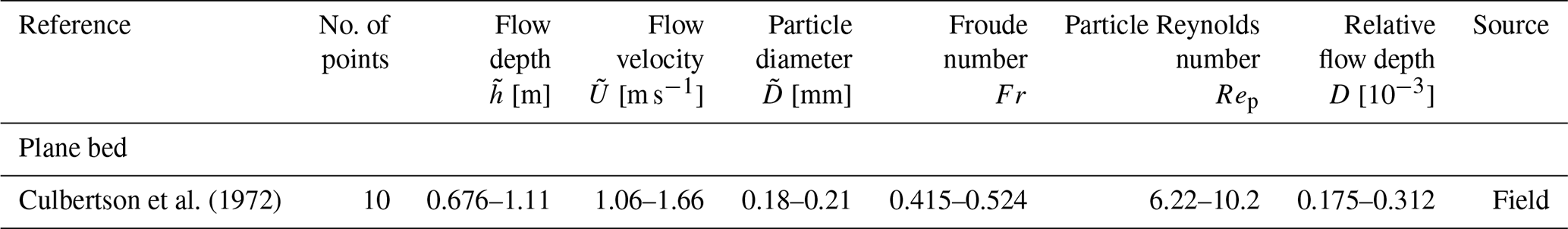
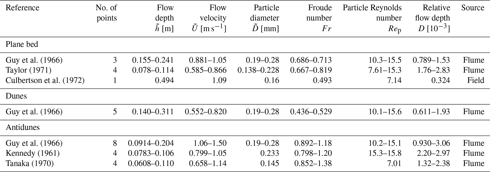
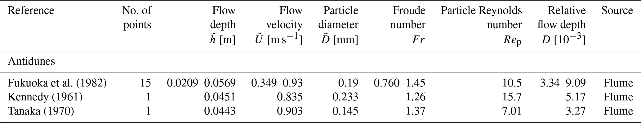
The stability diagrams were assessed using an observational dataset pertaining to open-channel flows compiled from the literature, as summarized in Tables A1–A5. We compiled from the literature a total of 56 sets of data for Fig. 2 and 59 sets of data for Fig. 3. The flow depth, flow velocity, and particle diameter range from 0.0209 to 1.11 m, 0.349 to 1.66 m s⁻¹, and 0.138 to 0.32 mm, respectively.

We used the data of plane beds in which the sediment transport mode could be identified, i.e., plane bed with suspension. We identified whether sediment particles were transported as suspended loads or not based on the suspended-sediment concentration. For comparison with the theoretical-analysis results, we used the data of dunes and antidunes with wavenumbers in the range of $\mathrm{0}<k\le \mathrm{1.5}$ for comparison. For Fig. 2, D of the data plotted in the diagram ranges from $D/\mathrm{3.16}$ to 3.16D. The data for which the particle Reynolds number ranges from $R{e}_{\mathrm{p}}/\mathrm{1.26}$ to 1.26Re_p were chosen to plot Fig. 3.

To calculate the particle Reynolds number, the kinematic viscosity ν was assumed as follows (van den Berg and van Gelder, 1993):

$$\begin{array}{}\text{(72)}& \mathit{\nu }=\left[\mathrm{1.14}-\mathrm{0.031}\left(T-\mathrm{15}\right)+\mathrm{0.00068}{\left(T-\mathrm{15}\right)}^{\mathrm{2}}\right]{\mathrm{10}}^{-\mathrm{6}},\end{array}$$

where T represents the water temperature in degrees Celsius. A value of 20 ^∘C was assumed for data when T was not reported.

3 Results

3.1 Re_p–Fr diagram

The contour maps of ω_i,max on the Re_p–Fr plane show that the stable region where the plane bed develops appears more extensive under hydraulic conditions with suspension than without suspension. (Fig. 2). In the case of the stability analysis without suspension, a stable region does not appear when $D/H={\mathrm{10}}^{-\mathrm{4}}$, and the growth rate decreases with increasing Re_p (Fig. 2a). For the phase diagram with $D={\mathrm{10}}^{-\mathrm{3}}$ and $D={\mathrm{10}}^{-\mathrm{2}}$, a stable region appears at $\mathrm{0.8}<\mathit{Fr}<\mathrm{1.2}$ (with $D={\mathrm{10}}^{-\mathrm{3}}$) and $\mathrm{0.7}<\mathit{Fr}<\mathrm{0.9}$ (with $D={\mathrm{10}}^{-\mathrm{2}}$) (Fig. 2c, e), and the growth rate increases with increasing Re_p.

The phase diagrams for the case of the stability analysis with suspension show that a stable region appears at $\mathrm{0.4}<\mathit{Fr}<\mathrm{0.9}$–1.0 (Fig. 2b, d, and f). Also, the growth rate at Fr>1 of the diagram with suspension is higher than that without suspension (Fig. 2a–d). In the case of shallow flow ($D={\mathrm{10}}^{-\mathrm{2}}$), the value of growth rate does not differ much between the diagrams with and without suspension (Fig. 2e and f).

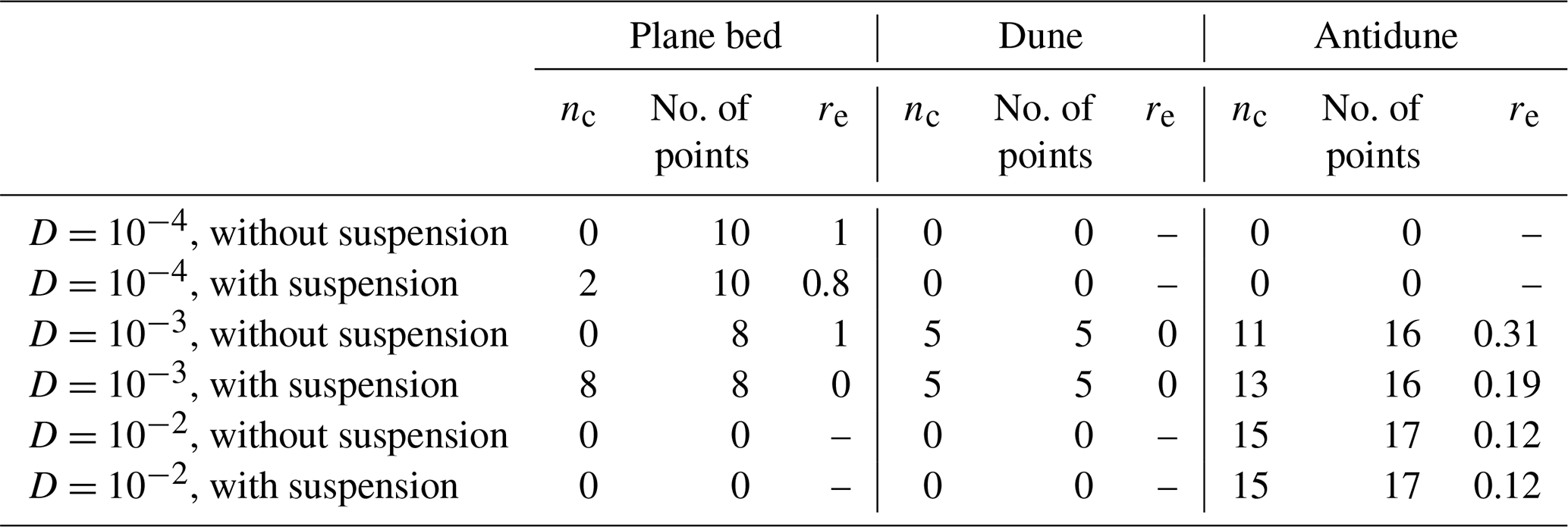
Comparing the results of theoretical analysis and the observational data, all the plane bed data are within unstable regions in the case without suspension (Fig. 2a and c). The analysis with suspension shows that all the plane bed data plot in the stable region when $D={\mathrm{10}}^{-\mathrm{3}}$ (Fig. 2d), whereas 2 data points out of 10 points plot in the stable region when $D={\mathrm{10}}^{-\mathrm{4}}$ (Fig. 2b). Table 1 also shows that the error rate, which denotes the number of plane bed data plotted in the unstable region, is smaller in the case with suspension than that in the case without suspension.

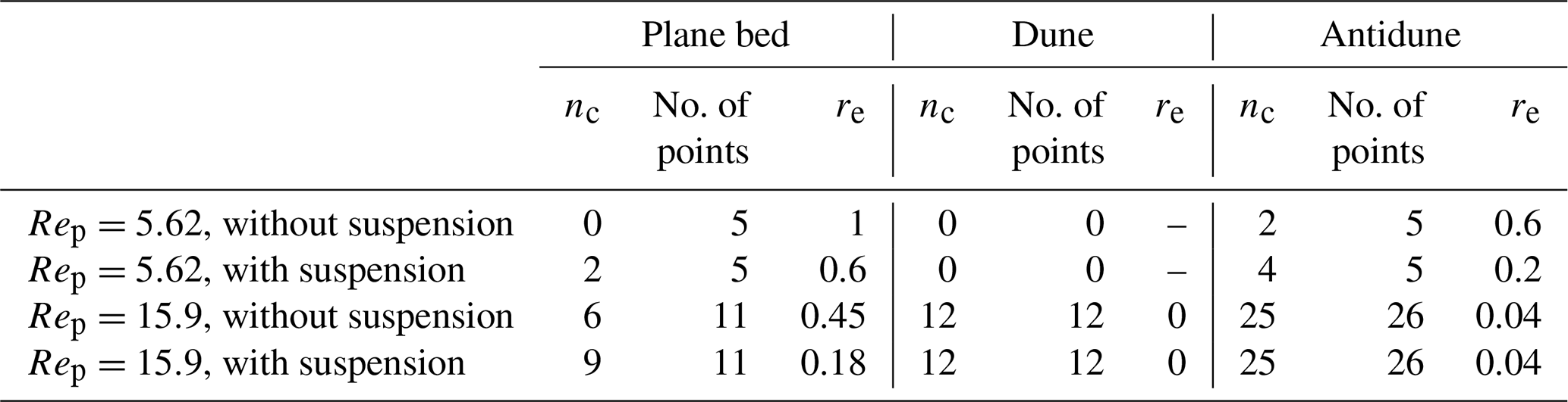
Table 1 Error rates for the case of fixed D. The parameter n_c denotes the number of correctly classified data points, and r_e is the error rate.

As expected, most dune and antidune data plot in the unstable region, whereas several data points of dunes and antidunes plot in the stable region in both cases with and without suspension (Fig. 2, Table 1).

3.2 D–Fr diagram

The contour maps of the maximum growth rate on the D–Fr plane also show that the stable region is larger in the diagram with suspension than in that without suspension (Fig. 3). For fine sediment, the upper limit of the stable region is smaller in the diagram with suspension than in that without suspension (Fig. 3a, b), whereas that does not much differ in the medium-sand case (Fig. 3c, d). Comparing with the observational data, most plane bed data plot in the stable region in the case of the stability analysis with suspension (Fig. 3). Also, most dune and antidune data plot in the unstable region in cases both with and without suspension (Fig. 3). The error rate for plane bed data decreased from 1 to 0.6 (Re_p=5.62) and 0.45 to 0.18 (Re_p=15.9) by adding the term of the suspended load (Table 2). For dunes and antidunes, the error rate does not differ between the cases with and without suspension, except for the antidune in the case of fine sediment, where r_e decreases from 0.6 to 0.2 (Table 2).

Table 2 Error rates for the case of fixed Re_p. The parameter n_c denotes the number of correctly classified data points, and r_e is the error rate.

4 Discussion

The role of suspended loads in the formation of plane beds and suppression of dune-scale instabilities is quantitatively illustrated as the broadening of the stable regions (Figs. 2 and 3). The stability diagrams show good agreement with the observational data of plane beds under flows with suspension. The transition from dunes to plane beds is explained by the spatial lag δ between the bed topography and the local sediment transport rate (Naqshband et al., 2014; van Duin et al., 2017). If the bed topography and sediment transport rate are entirely in phase (δ=0), dunes migrate downstream without growth or decay. The dune height increases and decreases when the maximum sediment transport rate occurs upstream (δ<0) and downstream (δ>0) of the dune crest, respectively. Kennedy (1963) introduced the spatial lag in his flow model to account for the bedform growth and decay, and subsequent research has investigated the effect of spatial lag on the bedform development (McLean, 1990; van Duin et al., 2017). Recently, Naqshband et al. (2017) quantitatively observed the positive spatial lag under suspended-load-dominated flows in their flume experiments. Our analyses confirm that suspended loads dampen the development of bed waves, thereby facilitating the formation of plane beds, and thus cannot be neglected in theoretical analyses for realistic predictions of bedforms.

We found that dunes are deformed under flows with suspended loads, although further work is needed to investigate the amplitudes of dunes under such conditions. Field surveys have indicated the existence of low-angle dunes in suspended-load-dominated rivers (Smith and McLean, 1977; Kostaschuk and Villard, 1996; Hendershot et al., 2016); moreover, flume experiments have indicated that dune height decreases with increasing suspended-load flux (Naqshband et al., 2017; Bradley and Venditti, 2019). Theoretical analyses in Fredsøe (1981) have also predicted a decrease in dune steepness under unsteady flows with suspension where the flow discharges were being increased. In future works, nonlinear analyses should be done to obtain the amplitudes of dunes under flows with suspended loads.

Ultimately, our linear analyses provide a possible explanation for the absence of dunes in turbidites: suspended loads suppress dune formation and facilitate plane bed formation. Previous research has suggested that the formation of dunes is suppressed due to the insufficient time for dune development (Walker, 1965), the hysteresis effect under waning flow conditions (Endo and Masuda, 1997), the turbulence suppression by high suspended-sediment concentrations (Lowe, 1988), the lack of a sharp near-bed density gradient (Arnott, 2012), and the effect of clay-sized sediment on bed rheology (Schindler et al., 2015). Although these interpretations could explain the absence of dune-scale cross-lamination in turbidites, we show that dune formation is suppressed without considering the above conditions. Although the above conditions may contribute to the deformation of dunes, instead, we propose that the development of dune-scale bed waves under turbidity currents is restricted by the presence of suspended loads. The model can be improved by the inclusion of such an effect in future studies.

5 Conclusions

We investigated the influence of suspended loads on the formation of plane beds under open-channel flows. The stability diagrams show that the stable region for finer sediments is wider in the diagram with suspension than that without suspension. Further, the published data of plane beds with suspension coincide well with the stability diagrams where the suspension was considered. Our theoretical analysis found that suspended loads promote the formation of plane beds and suppress the formation of dunes on the fine-grained bed. These results suggest that dune-scale cross-lamination is absent in turbidites because the development of dunes in turbidity currents is restricted by the presence of suspended loads. Additional theoretical work can be improved in future studies by the inclusion of possible mechanisms for the absence of dunes in turbidites.

Appendix A: Linear analysis

In Sect. 2.2.1–2.2.6, we formulate the hydrodynamics, the sediment transport model, and the basic state (Figs. A1 and A2). Here, we solve the equations obtained in the above sections.

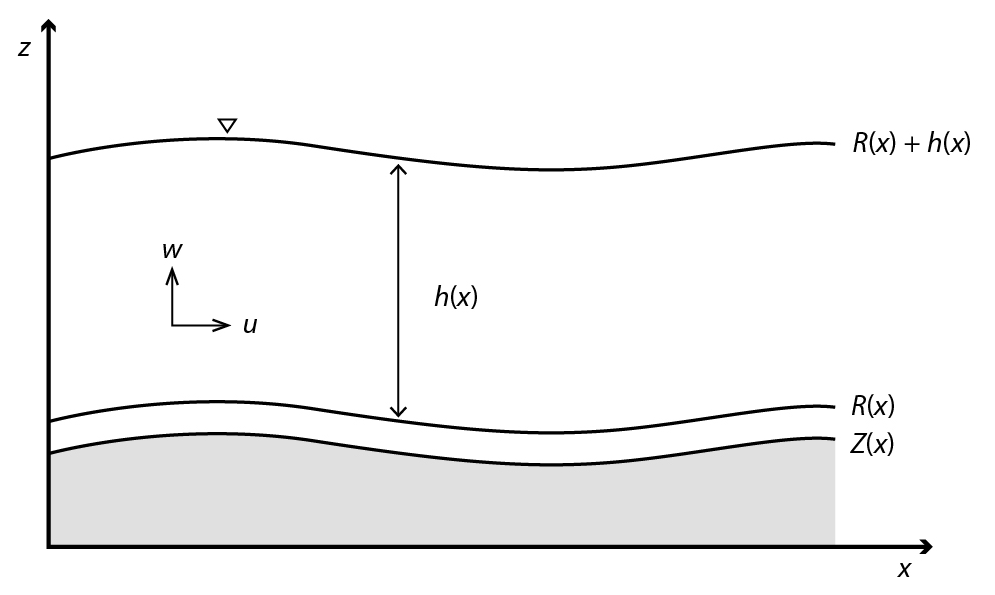
Figure A1 Conceptual diagram of the flow. The dimensionless parameters u and w are the flow velocities in the x and z directions, respectively; h is the flow depth; Z denotes the bed height; and R is the height of the reference level at which the flow velocity is assumed to vanish following a logarithmic law.

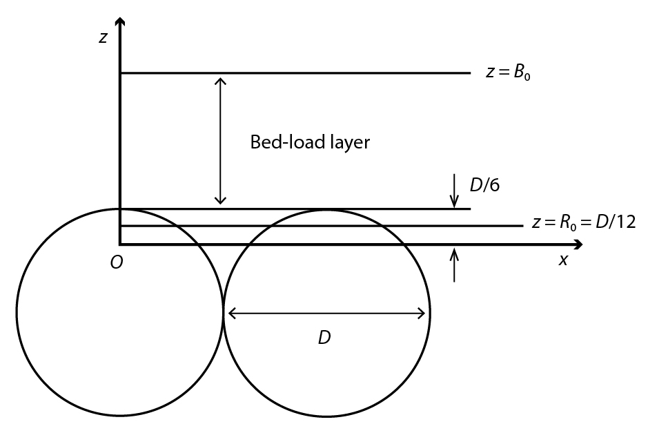
Figure A2 Conceptual diagram of the sediment bed. The origin of the z direction is denoted by O. The parameter D is the dimensionless diameter of a bed particle, B₀ is the height of the top of the bed-load layer in the basic state, and R₀ is the height of the reference level in the basic state.

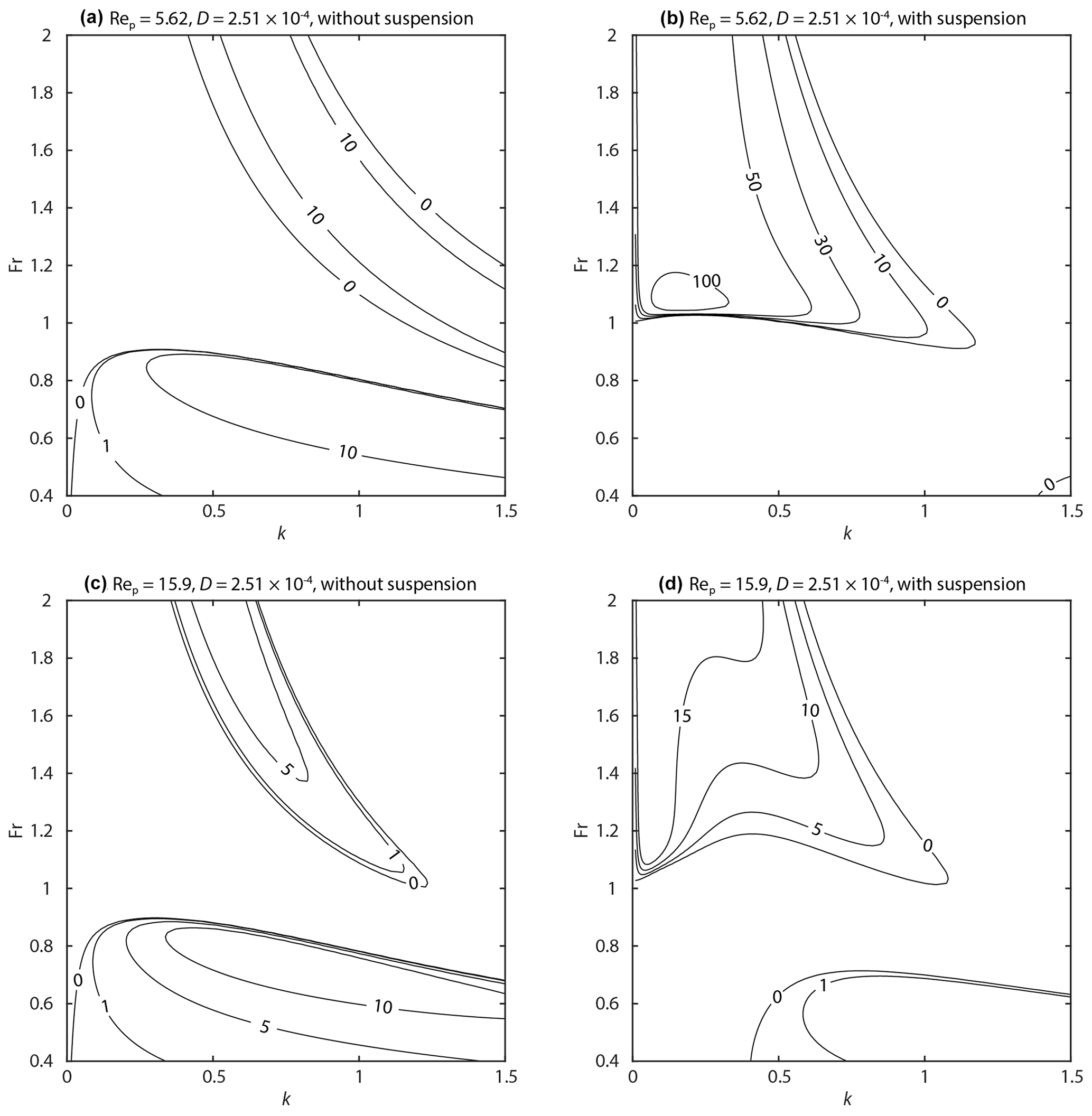
Figure A3 Contour map of perturbation growth rate ω_i. The dimensionless particle diameter D was set to $D=\mathrm{2.51}\times {\mathrm{10}}^{-\mathrm{4}}$. (a) Re_p=5.62 without suspension. (b) Re_p=5.62 with suspension. (c) Re_p=15.9 without suspension. (d) Re_p=15.9 with suspension.

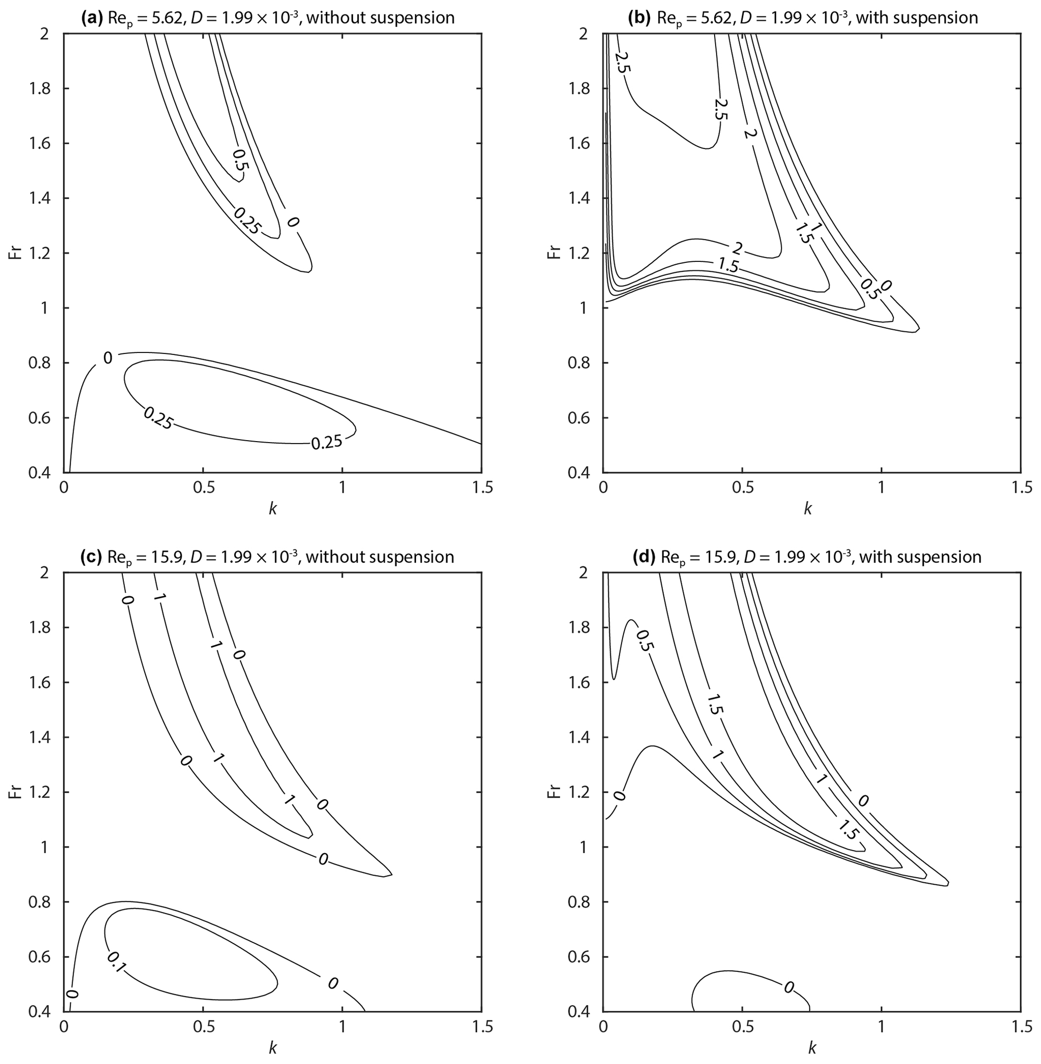
Figure A4 Contour map of perturbation growth rate ω_i. The dimensionless particle diameter D was set to $D=\mathrm{1.99}\times {\mathrm{10}}^{-\mathrm{3}}$. (a) Re_p=5.62 without suspension. (b) Re_p=5.62 with suspension. (c) Re_p=15.9 without suspension. (d) Re_p=15.9 with suspension.

Culbertson et al. (1972)Tanaka (1970)

Table A1 Summary of data used for the stability diagram with Re_p=5.62.

Bridge and Best (1988)Guy et al. (1966)Taylor (1971)Guy et al. (1966)Naqshband et al. (2014)Foley (1975)Guy et al. (1966)Kennedy (1961)

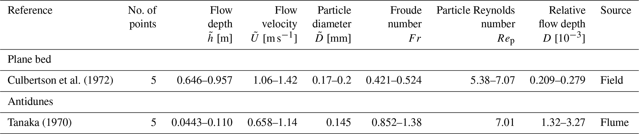
Table A2 Summary of data used for the stability diagram with Re_p=15.9.

Culbertson et al. (1972)

Table A3 Summary of data used for the stability diagram with $D={\mathrm{10}}^{-\mathrm{4}}$.

Guy et al. (1966)Taylor (1971)Culbertson et al. (1972)Guy et al. (1966)Guy et al. (1966)Kennedy (1961)Tanaka (1970)

Table A4 Summary of data used for the stability diagram with $D={\mathrm{10}}^{-\mathrm{3}}$.

Fukuoka et al. (1982)Kennedy (1961)Tanaka (1970)

Table A5 Summary of data used for the stability diagram with $D={\mathrm{10}}^{-\mathrm{2}}$.

We impose an infinitesimal perturbation on the basic state. All the variables are modified using a small amplitude A and a complex angular frequency of the perturbation ω as follows:

$$\begin{array}{}\text{(A1)}& \begin{array}{rl}& (\mathit{\psi },p,h,Z,R,B,c)=({\mathit{\psi }}_{\mathrm{0}},p_{\mathrm{0}},\mathrm{1},\mathrm{0},R_{\mathrm{0}},B_{\mathrm{0}},c_{\mathrm{0}})\\ & +A({\mathit{\psi }}_{\mathrm{1}},p_{\mathrm{1}},H_{\mathrm{1}},Z_{\mathrm{1}},R_{\mathrm{1}},B_{\mathrm{1}},c_{\mathrm{1}})\exp \left[i\left(k\mathit{\xi }-\mathit{\omega }t\right)\right].\end{array}\end{array}$$

The subscript 1 denotes a variable at 𝒪(A). By substituting Eq. (A1) into the governing equations and boundary conditions, we can obtain the following equations at 𝒪(A):

$$\begin{array}{}\text{(A2)}& {\displaystyle }{\mathcal{L}}^{\mathit{\psi }}\left(\mathit{\eta }\right){\mathit{\psi }}_{\mathrm{1}}\left(\mathit{\eta }\right)+{\mathcal{L}}^h\left(\mathit{\eta }\right)H_{\mathrm{1}}+{\mathcal{L}}^R\left(\mathit{\eta }\right)R_{\mathrm{1}}=\mathrm{0}\text{(A3)}& {\displaystyle }ik{p}_{\mathrm{1}}\left(\mathit{\eta }\right)+{\mathcal{P}}^{\mathit{\psi }}\left(\mathit{\eta }\right){\mathit{\psi }}_{\mathrm{1}}\left(\mathit{\eta }\right)+{\mathcal{P}}^h\left(\mathit{\eta }\right)H_{\mathrm{1}}+{\mathcal{P}}^R\left(\mathit{\eta }\right)R_{\mathrm{1}}=\mathrm{0}.\end{array}$$

Here, ℒ^ϕ and ${\mathcal{P}}^{\mathit{\varphi }}(\mathit{\varphi }=\mathit{\psi },h,R)$ are linear operators. The specific forms of ℒ^ϕ and 𝒫^ϕ are skipped herein. With the use of the boundary conditions (Eqs. 35 and 36), we get

$$\begin{array}{}\text{(A4)}& {\displaystyle }{\mathit{\psi }}_{\mathrm{1}}\left(\mathrm{1}\right)=\mathrm{0}\text{(A5)}& {\displaystyle }{p}_{\mathrm{1}}\left(\mathrm{1}\right)=\mathrm{0}\text{(A6)}& {\displaystyle }{\mathit{\psi }}_{\mathrm{1}}\left(\mathrm{0}\right)=\mathrm{0}\text{(A7)}& {\displaystyle }{\left.{\displaystyle \frac{\partial {\mathit{\psi }}_{\mathrm{1}}}{\partial \mathit{\eta }}}\right|}_{\mathit{\eta }=\mathrm{0}}=\mathrm{0}.\end{array}$$

Additionally, Eqs. (A3) and (A5) give

$$\begin{array}{}\text{(A8)}& {\mathcal{P}}^{\mathit{\psi }}\left(\mathrm{1}\right){\mathit{\psi }}_{\mathrm{1}}\left(\mathrm{1}\right)+{\mathcal{P}}^h\left(\mathrm{1}\right)H_{\mathrm{1}}+{\mathcal{P}}^R\left(\mathrm{1}\right)R_{\mathrm{1}}=\mathrm{0}.\end{array}$$

We employ a spectral collocation method using Chebyshev polynomials to solve the above differential equations. We expand ψ₁ using the Chebyshev polynomials as follows:

$$\begin{array}{}\text{(A9)}& {\mathit{\psi }}_{\mathrm{1}}=\sum _{n=\mathrm{0}}^N{a}_n{T}_n\left(\mathit{\zeta }\right),\end{array}$$

where a_n is the coefficient for the nth-order Chebyshev polynomial T_n, and ζ is the independent variable of the Chebyshev polynomials defined in the domain [$-\mathrm{1},\mathrm{1}$]. In this study, we transform ζ using the following equation to improve the calculation accuracy:

$$\begin{array}{}\text{(A10)}& \mathit{\zeta }=\mathrm{2}\left\{{\displaystyle \frac{\ln \left[(\mathit{\eta }+R_{\mathrm{0}})/R_{\mathrm{0}}\right]}{\ln \left[(\mathrm{1}+R_{\mathrm{0}})/R_{\mathrm{0}}\right]}}\right\}-\mathrm{1}.\end{array}$$

The above functions are substituted into Eq. (A2), and then we evaluate the equation at the Gauss–Labatte points, which are defined as

$$\begin{array}{}\text{(A11)}& {\mathit{\zeta }}_j=\cos \left({\displaystyle \frac{j\mathit{\pi }}{N+\mathrm{2}}}\right),j=\mathrm{1},\mathrm{2},\mathrm{\dots },N+\mathrm{1}.\end{array}$$

By combining the governing equations, boundary conditions, and closure assumptions, we obtain the following system of linear algebraic equations:

$$\begin{array}{}\text{(A12)}& \mathbf{La}=\mathbf{M}{R}_{\mathrm{1}},\end{array}$$

with

$$\begin{array}{}\text{(A13)}& {\displaystyle }\mathbf{L}=\left(\begin{array}{cccc}{T}_{\mathrm{0}}(-\mathrm{1})& \mathrm{\cdots }& T_N(-\mathrm{1})& \mathrm{0}\\ \stackrel{\mathrm{ˇ}}{\mathcal{h}}{T}_{\mathrm{0}}(-\mathrm{1})& \mathrm{\cdots }& \stackrel{\mathrm{ˇ}}{\mathcal{h}}{T}_N(-\mathrm{1})& \mathrm{0}\\ T_{\mathrm{0}}\left(\mathrm{1}\right)& \mathrm{\cdots }& T_N\left(\mathrm{1}\right)& \mathrm{0}\\ {\stackrel{\mathrm{ˇ}}{\mathcal{P}}}^{\mathit{\psi }}{T}_{\mathrm{0}}\left(\mathrm{1}\right)& \mathrm{\cdots }& {\stackrel{\mathrm{ˇ}}{\mathcal{P}}}^{\mathit{\psi }}{T}_N\left(\mathrm{1}\right)& {\stackrel{\mathrm{ˇ}}{\mathcal{P}}}^h\\ {\stackrel{\mathrm{ˇ}}{\mathcal{L}}}^{\mathit{\psi }}{T}_{\mathrm{0}}\left({\mathit{\zeta }}_{\mathrm{2}}\right)& \mathrm{\cdots }& {\stackrel{\mathrm{ˇ}}{\mathcal{L}}}^{\mathit{\psi }}{T}_N\left({\mathit{\zeta }}_{\mathrm{2}}\right)& {\stackrel{\mathrm{ˇ}}{\mathcal{L}}}^h\\ \mathrm{⋮}& \mathrm{\ddots }& \mathrm{⋮}& \mathrm{⋮}\\ {\stackrel{\mathrm{ˇ}}{\mathcal{L}}}^{\mathit{\psi }}{T}_{\mathrm{0}}\left({\mathit{\zeta }}_{N-\mathrm{2}}\right)& \mathrm{\cdots }& {\stackrel{\mathrm{ˇ}}{\mathcal{L}}}^{\mathit{\psi }}{T}_N\left({\mathit{\zeta }}_{N-\mathrm{2}}\right)& {\stackrel{\mathrm{ˇ}}{\mathcal{L}}}^h\end{array}\right)\text{(A14)}& {\displaystyle }\mathbf{a}=\left(a_{\mathrm{0}},a_{\mathrm{1}},\mathrm{\dots },a_N,D_{\mathrm{1}}\right)\text{(A15)}& {\displaystyle }\mathbf{M}=\left(\mathrm{0},\mathrm{0},\mathrm{0},{\stackrel{\mathrm{ˇ}}{\mathcal{P}}}^R,{\stackrel{\mathrm{ˇ}}{\mathcal{L}}}^h,\mathrm{\dots },{\stackrel{\mathrm{ˇ}}{\mathcal{L}}}^h\right),\end{array}$$

where a check mark denotes a linear operator associated with variable transformation from η to ζ. We obtain the following solution from Eq. (A12):

$$\begin{array}{}\text{(A16)}& \mathbf{a}={\mathbf{L}}^{-\mathrm{1}}\mathbf{M}{R}_{\mathrm{1}}.\end{array}$$

Additionally, Eqs. (A9) and (A16) give

$$\begin{array}{}\text{(A17)}& {\displaystyle }{\mathit{\psi }}_{\mathrm{1}}={\mathit{\psi }}_{\mathrm{1}}^{*}\left(\mathit{\eta }\right)R_{\mathrm{1}}\text{(A18)}& {\displaystyle }{H}_{\mathrm{1}}=H_{\mathrm{1}}^{*}{R}_{\mathrm{1}}.\end{array}$$

Similarly, we solve the eigenvalue problems for the sediment transport equations. By substituting Eq. (A1) into Eq. (24), we obtain the following equations of the order of 𝒪(A):

$$\begin{array}{}\text{(A19)}& {\mathcal{C}}^c{c}_{\mathrm{1}}\left(\mathit{\eta }\right)+{\mathcal{C}}^{\mathit{\psi }}\left(\mathit{\eta }\right){\mathit{\psi }}_{\mathrm{1}}\left(\mathit{\eta }\right)+{\mathcal{C}}^H{H}_{\mathrm{1}}+{\mathcal{C}}^R{R}_{\mathrm{1}}=\mathrm{0}.\end{array}$$

Based on Eqs. (A17) and (A18), we obtain

$$\begin{array}{}\text{(A20)}& {\mathcal{C}}^c{c}_{\mathrm{1}}\left(\mathit{\eta }\right)+\left({\mathcal{C}}^{\mathit{\psi }}\left(\mathit{\eta }\right){\mathit{\psi }}_{\mathrm{1}}^{*}\left(\mathit{\eta }\right)+{\mathcal{C}}^H{H}_{\mathrm{1}}^{*}+{\mathcal{C}}^R\right)R_{\mathrm{1}}=\mathrm{0}.\end{array}$$

The boundary conditions give

$$\begin{array}{}\text{(A21)}& {\displaystyle }{\mathcal{S}}^c{c}_{\mathrm{1}}\left(\mathrm{1}\right)+\left({\mathcal{S}}^{\mathit{\psi }}\left(\mathrm{1}\right){\mathit{\psi }}_{\mathrm{1}}^{*}\left(\mathrm{1}\right)+{\mathcal{S}}^H{H}_{\mathrm{1}}^{*}+{\mathcal{S}}^R\right)R_{\mathrm{1}}=\mathrm{0}\text{(A22)}& {\displaystyle }{\mathcal{B}}^c{c}_{\mathrm{1}}\left(\mathrm{0}\right)+\left({\mathcal{B}}^{\mathit{\psi }}\left(\mathrm{0}\right){\mathit{\psi }}_{\mathrm{1}}^{*}\left(\mathrm{0}\right)+{\mathcal{B}}^H{H}_{\mathrm{1}}^{*}+{\mathcal{B}}^R\right)R_{\mathrm{1}}=\mathrm{0}.\end{array}$$

Here, 𝒞^ϕ, 𝒮^ϕ, and ${\mathcal{B}}^{\mathit{\varphi }}(\mathit{\varphi }=\mathit{\psi },h,R,c)$ are the linear operators.

We expand c₁ using Chebyshev polynomials as follows:

$$\begin{array}{}\text{(A23)}& c_{\mathrm{1}}=\sum _{n=\mathrm{0}}^N{b}_n{T}_n\left(\mathit{\zeta }\right).\end{array}$$

The system is evaluated at the Gauss–Labatte points, and then we obtain

$$\begin{array}{}\text{(A24)}& \mathbf{Kb}=\mathbf{N}{R}_{\mathrm{1}},\end{array}$$

with

$$\begin{array}{}\text{(A25)}& \mathbf{K}=\left(\begin{array}{ccc}{\stackrel{\mathrm{ˇ}}{\mathcal{B}}}^c{T}_{\mathrm{0}}(-\mathrm{1})& \mathrm{\cdots }& {\stackrel{\mathrm{ˇ}}{\mathcal{B}}}^c{T}_N(-\mathrm{1})\\ {\stackrel{\mathrm{ˇ}}{\mathcal{S}}}^c{T}_{\mathrm{0}}\left(\mathrm{1}\right)& \mathrm{\cdots }& {\stackrel{\mathrm{ˇ}}{\mathcal{S}}}^c{T}_N(-\mathrm{1})\\ {\stackrel{\mathrm{ˇ}}{\mathcal{C}}}^c{T}_{\mathrm{0}}\left({\mathit{\zeta }}_{\mathrm{1}}\right)& \mathrm{\cdots }& {\stackrel{\mathrm{ˇ}}{\mathcal{C}}}^c{T}_N\left({\mathit{\zeta }}_{\mathrm{1}}\right)\\ \mathrm{⋮}& \mathrm{\ddots }& \mathrm{⋮}\\ {\stackrel{\mathrm{ˇ}}{\mathcal{C}}}^c{T}_{\mathrm{0}}\left({\mathit{\zeta }}_{N-\mathrm{1}}\right)& \mathrm{\cdots }& {\stackrel{\mathrm{ˇ}}{\mathcal{C}}}^c{T}_N\left({\mathit{\zeta }}_{N-\mathrm{1}}\right)\end{array}\right)\end{array}$$

$$\begin{array}{}\text{(A26)}& {\displaystyle }\mathbf{b}=\left(b_{\mathrm{0}},b_{\mathrm{1}},\mathrm{\dots },b_N\right)\text{(A27)}& {\displaystyle }\mathbf{N}=-\left(\begin{array}{c}{\stackrel{\mathrm{ˇ}}{\mathcal{B}}}^{\mathit{\psi }}{\mathit{\psi }}_{\mathrm{1}}^{*}(-\mathrm{1})+{\stackrel{\mathrm{ˇ}}{\mathcal{B}}}^h{H}_{\mathrm{1}}^{*}+{\stackrel{\mathrm{ˇ}}{\mathcal{B}}}^R\\ {\stackrel{\mathrm{ˇ}}{\mathcal{S}}}^{\mathit{\psi }}{\mathit{\psi }}_{\mathrm{1}}^{*}\left(\mathrm{1}\right)+{\stackrel{\mathrm{ˇ}}{\mathcal{S}}}^h{H}_{\mathrm{1}}^{*}+{\stackrel{\mathrm{ˇ}}{\mathcal{S}}}^R\\ {\stackrel{\mathrm{ˇ}}{\mathcal{C}}}^{\mathit{\psi }}{\mathit{\psi }}_{\mathrm{1}}^{*}\left({\mathit{\zeta }}_{\mathrm{1}}\right)+{\stackrel{\mathrm{ˇ}}{\mathcal{C}}}^h{H}_{\mathrm{1}}^{*}+{\stackrel{\mathrm{ˇ}}{\mathcal{C}}}^R\\ \mathrm{⋮}\\ {\stackrel{\mathrm{ˇ}}{\mathcal{C}}}^{\mathit{\psi }}{\mathit{\psi }}_{\mathrm{1}}^{*}\left({\mathit{\zeta }}_{N-\mathrm{1}}\right)+{\stackrel{\mathrm{ˇ}}{\mathcal{C}}}^h{H}_{\mathrm{1}}^{*}+{\stackrel{\mathrm{ˇ}}{\mathcal{C}}}^R\end{array}\right).\end{array}$$

The coefficient b_n is derived as

$$\begin{array}{}\text{(A28)}& \mathbf{b}={\mathbf{K}}^{-\mathrm{1}}\mathbf{N}{R}_{\mathrm{1}}.\end{array}$$

Therefore, the following equation is obtained:

$$\begin{array}{}\text{(A29)}& c_{\mathrm{1}}\left(\mathit{\eta }\right)=c_{\mathrm{1}}^{*}\left(\mathit{\eta }\right)R_{\mathrm{1}}.\end{array}$$

By substituting Eqs. (A17), (A18), and (A29) into Exner's equation (Eq. 61), the complex angular frequency ω is obtained in the following form:

$$\begin{array}{}\text{(A30)}& \mathit{\omega }=\mathit{\omega }(k,Fr,C_z,R{e}_{\mathrm{p}})={\mathit{\omega }}_{\mathrm{r}}+i{\mathit{\omega }}_i,\end{array}$$

where ω_i corresponds to the growth rate of the perturbation.

Here, using $R{e}_{\mathrm{p}}=R{e}_{\mathrm{p}}\left(D\right)=R{e}_{\mathrm{p}}(\stackrel{\mathrm{̃}}{D},{\stackrel{\mathrm{̃}}{h}}_{\mathrm{0}})$ (Eq. 27) and $C_z=C_z\left(R_{\mathrm{0}}\right)=C_z(\stackrel{\mathrm{̃}}{D},{\stackrel{\mathrm{̃}}{h}}_{\mathrm{0}})$ (Eq. 52), we can rewrite Eq. (A30) as

$$\begin{array}{}\text{(A31)}& \mathit{\omega }=\mathit{\omega }\left(k,Fr,\stackrel{\mathrm{̃}}{D},{\stackrel{\mathrm{̃}}{h}}_{\mathrm{0}}\right).\end{array}$$

Thus, we can obtain the growth rate ω_i as a function of k for a given combination of Fr, $\stackrel{\mathrm{̃}}{D}$, and ${\stackrel{\mathrm{̃}}{h}}_{\mathrm{0}}$.