the Creative Commons Attribution 4.0 License.
the Creative Commons Attribution 4.0 License.
 | 05 Jan 2024
Bedload transport fluctuations, flow conditions, and disequilibrium ratio at the Swiss Erlenbach stream: results from 27 years of high-resolution temporal measurements
Dieter Rickenmann
Based on measurements with the Swiss plate geophone system with a 1 min temporal resolution, bedload transport fluctuations were analysed as a function of the flow and transport conditions in the Swiss Erlenbach stream. The study confirms a finding from an earlier event-based analysis of the same bedload transport data, which showed that the disequilibrium ratio of measured to calculated transport rate (disequilibrium condition) influences the sediment transport behaviour. To analyse the transport conditions, the following elements were examined to characterise bedload transport fluctuations: (i) the autocorrelation coefficient of bedload transport rates as a function of lag time (memory effect), (ii) the critical discharge at the start and end of a transport event, (iii) the variability in the bedload transport rates, and (iv) a hysteresis index as a measure of the strength of bedload transport during the rising and falling limb of the hydrograph. This study underlines that above-average disequilibrium conditions, which are associated with a larger sediment availability on the streambed, generally have a stronger effect on subsequent transport conditions than below-average disequilibrium conditions, which are associated with comparatively less sediment availability on the streambed. The findings highlight the important roles of the sediment availability on the streambed, the disequilibrium ratio, and the hydraulic forcing in view of a better understanding of the bedload transport fluctuations in a steep mountain stream.
- Article
(6013 KB) - Full-text XML
-
Supplement
(1086 KB) - BibTeX
- EndNote


A recent comprehensive review of bedload transport fluctuations was compiled by Ancey (2020a, b). He concluded that predictions of transport levels from bedload transport relationships are typically associated with an uncertainty of (at least) about 1 order of magnitude and that morphodynamic models fail to explain bedform evolution without the use of additional assumptions (Ancey, 2020a). He also noted that bedload transport rates depend on many processes that vary in time and space and are interrelated (Ancey, 2020b). Some aspects influencing the fluctuations in bedload transport, apart from the primary control by hydraulic forcing, are summarised below, focusing on those that are relevant for this study.
Possible reasons for the variability in bedload transport rates were previously discussed in Rickenmann (2020). One reason is related to changes in bed evolution as a result of bedload transport affecting the critical Shields stress necessary for the start of bedload transport, such as changes in packing arrangement, grain sizes of the bed surface, roughness, imbrication and orientation of the particles, cluster structure, and armour layer configuration (e.g. Church, 2006; Piedra et al., 2012; Mao, 2012; Guney et al., 2013; Roth et al., 2017). A second reason is the stabilisation of the bed surface during low-flow periods without bedload transport (inter-event flows) and during flow periods with only weak transport, leading to an increase in critical Shields stress or a reduction in sediment transport (e.g. Paphitis and Collins, 2005; Haynes and Pender, 2007; Ockelford et al., 2019). Such a stabilisation of the bed surface was also confirmed for the Swiss Erlenbach stream (Masteller et al., 2019). A third reason for the transport variability is sediment availability on the bed surface, caused either by high-discharge events breaking up channel bed structures (Turowski et al., 2009; Yager et al., 2012) or by higher rates of upstream sediment supply resulting both in more mobile sediment and thus in lower critical Shields stresses (Dietrich et al., 1989; Recking, 2012; Bunte et al., 2013; Rickenmann, 2020). Based on flume experiments, An et al. (2021) examined the effect of antecedent conditioning flows with different durations (stress history) followed by a hydrograph with increasing discharge (only rising limb) and sediment input on changes in bed elevation, surface grain size, and bedload transport. They concluded that the effect of stress history on sediment transport rate is important at the beginning of a hydrograph and diminishes with the increase in discharge and sediment supply, suggesting a loss of memory of stress history under high-flow conditions.
The correlation between bedload transport and water discharge was found to clearly increase when averaging measurements of bedload transport over increasing time periods (Downs et al., 2016; Lenzi et al., 2004; Recking et al., 2012; Rickenmann, 1994, 2016, 2018; Rickenmann and McArdell, 2008). Based on continuous bedload transport measurements with the Swiss plate geophone (SPG) system, Rickenmann (2018) reported a substantial increase in the correlation coefficient R between transport rate and discharge for minimum aggregation times of about 1–2 h, which integrates over typical short-term fluctuations of 15–35 min of bedload transport rates in natural gravel bed streams. Such short-term fluctuations were found by assessing the temporal variability in bedload transport at a timescale of less than 1 h for the Drava river in Austria by Habersack et al. (2012) and for the Elwha River in the US by Hilldale (2015). In both studies, SPG measurements were used with a 1 min recording interval of geophone impulses, which showed a periodicity of bedload peaks ranging from 15 to 35 min, based on moving 5 min average values. Fluctuations with a periodicity of 14 to 35 min were also found in a field study of the Turkey Brook in England (Reid and Frostick, 1986) and in flume experiments (Kuhnle and Southard, 1988, Strom et al., 2004) for a variety of hydraulic and sediment supply conditions. Moving bed load sheets or the formation and destruction of gravel clusters were suggested as possible reasons for such fluctuations (Hilldale, 2015; Kuhnle and Southard, 1988).
Liébault et al. (2022) investigated the behaviour of seasonal bedload pulses in a small alpine catchment, and they concluded that the mean bedload response of the alluvial system is strongly controlled by sediment storage within the channel system, as evidenced by larger bedload fluxes at the catchment outlet during degradational phases in the channel upstream. Brenna and Surian (2023) concluded from a field study that fluxes of coarse sediment in a mountain stream in northern Italy recently affected by a large flood could be considerably higher than those normally expected because of the high availability of fresh and unstructured sediment within the channel. A similar explanation of such a memory effect was proposed by Turowski et al. (2009), Yager et al. (2012), and Masteller et al. (2019), who observed that extreme flood events in mountain streams can destabilise the channel bed and increase sediment availability and following fluxes.
Autocorrelation analysis was used to assess memory effects in bedload transport time series. Elgueta Astaburuaga et al. (2018) analysed the effect of sediment supply on sediment mobility for a poorly sorted experimental bed, and they suggested that large sediment pulses may increase the strength and persistence of autocorrelation in bedload rate time series. In another flume study, Saletti et al. (2015) found from autocorrelation analysis that memory is grain-size-dependent, highlighting the importance of fractional transport data for an accurate description of bed load dynamics. Masteller et al. (2019) showed for field data from the Erlenbach stream that the critical Shields stress at the start of an event remained significantly autocorrelated over up to about 10 transport events. Rickenmann (2020) found a similar memory effect for the Erlenbach for critical Shields stress at the end of an event and for the disequilibrium ratio.
Continuous and longer time series of bedload transport measurements are still scarce for field situations. Therefore, the majority of studies on fluctuations in bedload transport rely on flume experiments. Mettra (2014) investigated bedload transport fluctuations with a series of flume experiments and considered the effect of varying sediment input at the upstream end of the flume. For increasing values of unit bedload transport rates qb at the flume outlet, varying from about 0.33 to 600 g s−1 m−1, he found an almost linear decrease in the coefficient of variation (cv) of qb (i.e. standard deviation of qb divided by mean of qb) from about 10 to 0.1. He also observed that intermittency of transport increased with increasing channel steepness, decreasing sediment supply, and decreasing bulk flow energy. Furthermore, he found that lower sediment supply, higher channel slope, and lower Shields stress lead to more intense hysteretic effects. Singh et al. (2009) performed flume experiments with qb= 0.36 and 730 g s−1 m−1 and determined cv values of 0.98 and 0.76 for aggregation times of 1 min. From their flume experiments, Kuhnle and Southard (1988) determined for 1 min sampling times for qb = 52 to 541 g s−1 m−1 cv values from 0.33 to 0.5 and for qb= 6000 g s−1 m−1 a cv value of 0.13. Ma et al. (2014) performed flume experiments with spherical beads, and for an integration time of 1 min they measured a mean bedload flux of 1.1 particles s−1 and determined a cv value of 1.29.
Regarding direct bedload measurements, Kuhnle and Willis (1998) used data from Goodwin creek in the USA and determined for qb= 7.4 to 550 g s−1 m−1 and a 1 min sampling time cv values from 2.42 to 0.78, with the bulk of values varying between 1 and 2; they also found a tendency for the cv values to decrease with increasing bedload transport rates. Other field studies cited below were based on impact plate measurements with the SPG system. For the Elwha River in the USA, Hilldale (2015) analysed impulse counts with a recording interval of 1 min for two different events and found a cv value of 0.92 and of 0.78, respectively, for a unit flow discharge of about 2.1 m3 s−1 m−1. Ancey and Pascal (2020) analysed bedload transport measurements in the Navisence River in Switzerland, and for an approximately constant unit flow discharge of about 1.2 m3 s−1 m−1 over 1 h and a mean value of qb= 39 g s−1 m−1 the resulting cv value for a 1 min sampling time was 0.41.
A comprehensive review of the hysteresis behaviour of sediment transport rates in alluvial streams was made by Gunsolus and Binns (2018), who concluded that lower-magnitude hydrographs resulted in more pronounced hysteresis than larger-magnitude hydrographs. Clockwise hysteresis (with higher transport rates on the rising than on the falling hydrograph limb) has often been associated with a gradual decrease in sediment availability or early exhaustion of sediment sources (Pretzlav et al., 2020; Mao et al., 2019; Rovira and Batalla, 2006; Gao and Pasternack, 2007). Anticlockwise hysteresis was suggested to result from temporal lags as bedforms adjust to changing discharge (Bombar et al., 2011; Martin and Jerolmack, 2013) or from the destabilisation of surface structures during hydrograph rising limbs (Kuhnle, 1992).
The objective of this study is to examine the bedload transport fluctuations as a function of the flow and transport conditions in the Swiss Erlenbach stream. The study is based on 27 years of 1 min time series of bedload transport rates, measured with the SPG system, for the same 522 flood events which were used previously for the analysis of event-based transport characteristics (Rickenmann, 2020). The disequilibrium ratio was determined as the ratio of measured to calculated transport rate, similar to the definition in Rickenmann (2020). This new study focuses on the following elements that characterise bedload transport fluctuations: (i) the autocorrelation coefficient of bedload transport rates as a function of lag time, (ii) the critical discharge at the start and end of a transport event, (iii) the coefficient of variation of the bedload transport rates, and (iv) a hysteresis index as a measure of the strength of clockwise or anticlockwise transport behaviour. These elements are analysed and discussed in the context of variations in discharge, bedload transport level, and disequilibrium ratio. The findings highlight the important roles of the sediment availability on the streambed, the disequilibrium ratio, and the hydraulic forcing in view of a better understanding of the bedload transport fluctuations in a steep mountain stream.
2.1 The Erlenbach catchment
The Erlenbach catchment is situated in the Alptal valley in the pre-Alps of central Switzerland and has an area of ∼ 0.7 km2 (Rickenmann et al., 2012). Geologically, the Erlenbach basin is located in a flysch zone; creeping and sliding slopes along most of the channel length provide a persistent high supply of sediment to the channel (Schuerch et al., 2006; Golly et al., 2017). The hydrology of the Erlenbach catchment is characterised by both frequent high-intensity storms in summer with discharge events of short duration and some snowmelt events in spring. Annual precipitation totals are around 2300 mm (Rickenmann and McArdell, 2007).
The stream gradient is 18 % on average and 10.5 % along the 50 m long natural reach immediately upstream of the gauging site (Fig. 1). The Erlenbach has a pronounced step–pool–riffle morphology (Rickenmann and McArdell, 2007; Turowski et al., 2009). The channel is situated in alluvial materials, originating from weathered flysch bedrock, with grain sizes ranging from clay to boulders. Most of the catchment is on a large landslide complex, and the left bank is particularly active in a reach 500 m upstream of the gauging station (Schuerch et al., 2006). In this reach, the steps – composed of both coarse particles and large wood – are up to 2 m high, with a mean step height of 0.7 m and a mean step spacing of almost 8 m (Molnar et al., 2010). Bedload transport events occur on average about 20 times per year. The three largest sediment transport events had peak discharges of about 10 m3 s−1 or more and resulted in transported sediment volumes (including fine material) of more than 1000 m3 (Rickenmann, 2020).
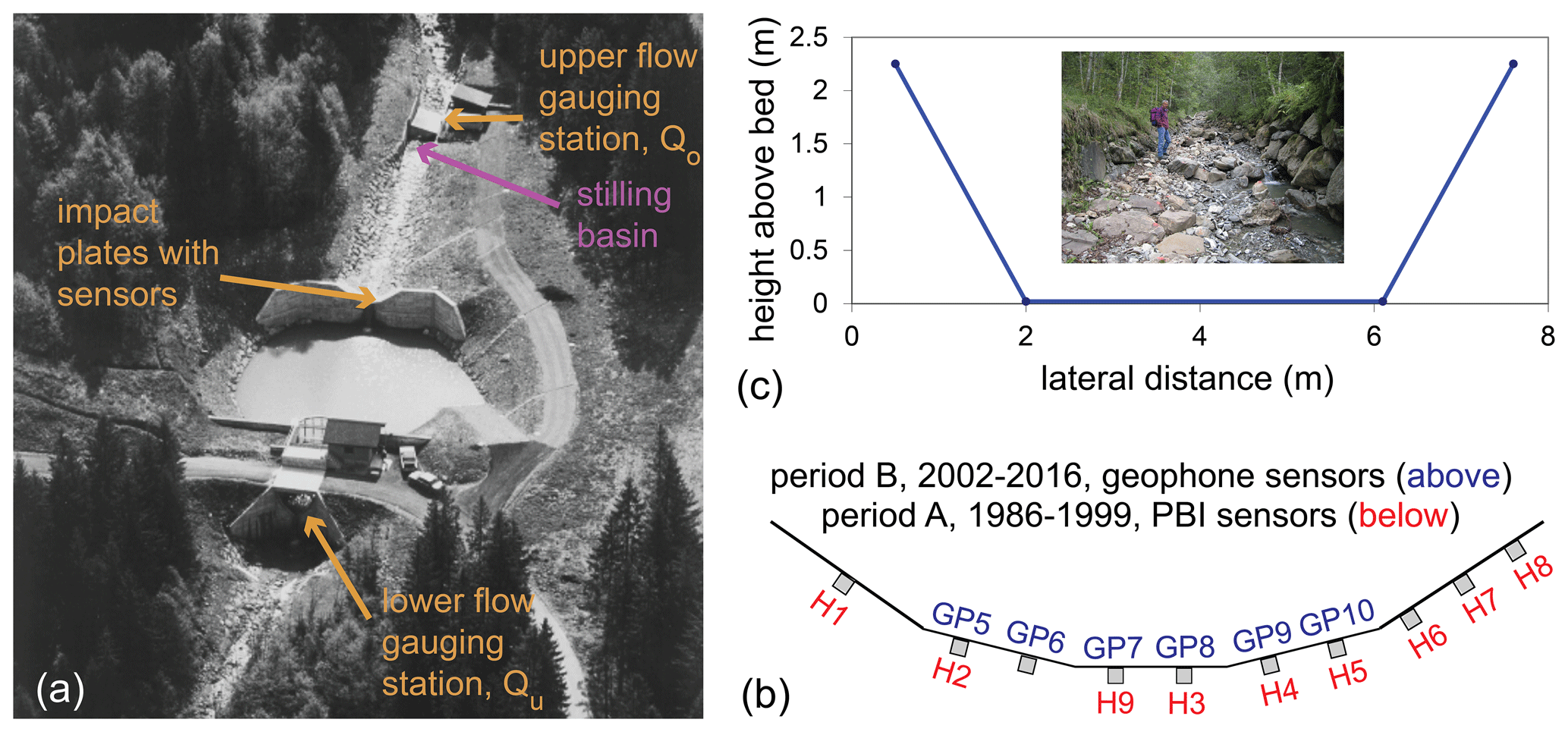
Figure 1(a) Surrogate bedload impact plates, sediment retention basin, and two gauging sites at the Erlenbach stream. (b) Schematic cross-section, with downstream view of the lateral distribution of PBI sensors (Hi) during period A (1986–1999) and of geophone sensors (GPi) during period B (2002–2016), where i denotes the sensor number. (c) Symmetrical, trapezoidal cross-section used for the hydraulic and bedload transport calculations, with a bottom width bw= 4.1 m and a lateral slope of 1.5:1; this cross-section represents the natural reach upstream of the measuring installations, with the banks protected by a riprap construction (inset photo, upstream view). (Modified from Rickenmann, 2020).
2.2 Bedload transport measurements
Near the catchment outlet there is a sediment retention basin (Fig. 1a). Downstream of the lowest natural channel reach, an artificial channel with embedded riprap leads to a large check dam, forming the upstream end of this retention basin. Since 1986 several adjacent steel plates with impact sensors are embedded in the check dam to continuously measure bedload transport. These sensors record the vibrations resulting from the movement of gravel-sized and larger particles over a steel plate (Rickenmann and McArdell, 2007). From 1986 to 1999 piezoelectric impact sensors (PBIs), developed in-house, were used. Because of deterioration of these PBI sensors, they were replaced by geophone sensors from 2000 onwards (Rickenmann, 2017). The bedload measurements with both sensors result in a very similar signal response (Rickenmann et al., 2012). The minimum grain size that can be detected by both systems is about 10 mm (Rickenmann and McArdell, 2007; Rickenmann et al., 2012; Rickenmann et al., 2014; Wyss et al., 2016a, b; Nicollier et al., 2022). A vibration sensor is fixed from underneath to the centre of a steel plate. The steel plates have standard dimensions of L × B × T = 358 × 496 × 15 mm, where L is the downstream length, B is the transversal width, and T is the thickness of the plate.
For the calibration of the surrogate measuring system, the summary value of the impulse counts is used in this study: whenever the voltage of the raw signal exceeds a preselected threshold value At (in volts), this is recorded as an impulse, and the summed impulses are stored. The threshold value to record impulses was set to At= 0.2 V for the PBI and to At= 0.1 V for the geophone sensors. During bedload-transporting flood events, the summed impulse counts IMP were recorded in minute intervals. The use of a threshold essentially eliminates the noise of the signal. A linear relation between impulses and bedload mass transported over a plate was found to apply quite well at several field sites, including the Erlenbach (Rickenmann et al., 2012, 2014, 2020; Wyss et al., 2016a, c; Nicollier et al., 2021). For period A with the PBI sensors (1986–1999), a total of 9 plates were equipped with a sensor, and the lateral distribution of these sensors is illustrated in Fig. 1b. There is an asymmetrical lateral distribution of bedload transport intensities, due to an offset of the centreline axes of the approach flow channel with respect to the position of the check dam upstream of the retention basin. As a result, most signal was recorded by sensor H3, followed by sensors H4 and H9 (Rickenmann and McArdell, 2007). For period B with the geophone sensors (2002–2016), a total of six plates were equipped with a sensor, and the lateral distribution of the devices is illustrated in Fig. 1b. A similar asymmetrical lateral distribution of bedload transport intensities was evident also for this period.
The linear calibration relation for the impact plate measurements used to convert the number of impulses into a channel-wide bedload transport rate Qb, including grains larger than 4 mm for both periods, was determined as
where kisp denotes the individual calibration coefficients determined for each survey interval of the deposits in the sediment retention basin, ρd= 1750 kg m−3 is the mean bulk density of the deposits (Rickenmann and McArdell, 2007), the coefficient fc= 0.5 accounts for an estimated 50 % of particles having a grain size larger than 10 mm (Rickenmann and McArdell, 2007), and the coefficient 60 is used to convert the 1 min IMP readings to a mean value of Qb expressed in kg s−1. Finally, the coefficient mfg is used to account for the fraction of particles in the range of “fine gravel”, i.e. for 4 mm < D < 10 mm, where D is particle size. The value of mfg was estimated with the aid of the Erlenbach moving basket system to collect bedload samples (Rickenmann et al., 2012). The standard mesh size of the metal basket is 10 mm. For 11 samples from 2013 to 2017 a second layer of a metal wire net with a mesh size of 2 mm was inserted into one of the three baskets. From these samples a mean value of mfg= 1.54 was determined to correct for non-measured particles in the range 4 mm < D < 10 mm with the IMP counts. The individual mfg values showed a slight decrease with increasing transport rate Qb, whereby Qb was smaller than 1 kg s−1 for all 11 samples. Thus, the lumped factor fg= 22.46 in Eq. (1) accounts for the mean bulk density of the deposits in the sediment retention basin, the estimation of the proportion of particles larger than 2 mm in the deposits, and the conversion of the 1 min IMP readings to a mean value of Qb expressed in kg s−1. The originally measured Qb values also include zero values and are termed Qbz henceforth (for comparison with a full time series QbM for which zero values were replaced with non-zero values, see Sect. 2.6).
For period A, only the recordings with sensor plate H3 (Fig. 1b) were used to determine the individual calibration coefficients kisp because data from other sensors were sometimes missing. For period B, the sum of the impulses from sensor plates GP6, GP7, GP8, GP9, and GP10 (Fig. 1b) were used to determine the individual calibration coefficients kisp; data from the sensor plate GP5 were not included because this sensor malfunctioned for some later years. The resulting calibration coefficients kisp are reported in the Supplement (Table S1) of Rickenmann (2020).
2.3 Discharge measurements
There are two discharge gauging stations near the sediment retention basin, which is close (∼ 100 m) to the outlet of the catchment. The so-called lower station at the outflow from the (dammed) sediment retention basin consists of a double triangular profile; the associated stage–discharge relationship (discharge Qu) was calibrated with a physical model before construction and is therefore quite reliable also during flood flows. The upper discharge measurement station is located between the end of the natural channel and the retention basin, and it consists of an asymmetrical cross-section in a concrete channel; the associated stage–discharge relationship (discharge Qo) was calibrated based on dye and salt tracer measurements, especially for small and medium discharges, but including values up to 5 m3 s−1. The location of the two gauging sites is illustrated in Fig. 1a and in Beer et al. (2015, Fig. 2 therein).
For the sediment-transporting flood events, discharges were in the range of 0.1 to 15 m3 s−1 (Rickenmann, 1997; Turowski et al., 2009). The definition of a sediment-transporting flood event is based on the recording of the bedload transport activities. During such events, level measurements are available with a recording interval of 1 min for both stream gauging sites. More details on the bedload transport criteria to start and end the recording of an event are given in the supporting information for Rickenmann (2020, Supplement Sect. S2 therein).
Generally, I used the Qo values from the upper gauging station in this study. Due to uncertainty in the level–discharge relationship for some (limited) periods, the Qo values from the upper gauging station were replaced by Qu values from the lower gauging station. I estimated the uncertainty in the Qo values to be 15 % or slightly less, similarly to Beer et al. (2015). More details on the discharge measurements are given in the supporting information (Sect. S3) of Rickenmann (2020). For simplicity, measured discharges used in the further analysis are labelled as Q values in the following text.
Immediately downstream of the upper gauging site, the flow drops over an engineered overfall structure (∼ 1 m high) into a shallow stilling basin (∼ 4 m × 4 m × 0.3 m depth), then enters a fairly smooth ∼ 30 m engineered concrete reach with large blocks embedded in cement before reaching the impact plates (Fig. 1a; see also Roth et al., 2017, Fig. 1 therein). This stilling basin slightly delays the sediment transfer between the (upper) gauging station and the impact plates.
2.4 Sediment-transporting flood events
The delineation of sediment-transporting flood events is described in detail in Rickenmann (2020). On some days with bedload transport, the IMP counts ceased for minutes to hours and restarted again. A minimum inter-flood duration time of 75 min (without any transport signal) was used to separate different transport events, which is of the order of the duration of a typical flood event (see below). Furthermore, the smallest events were excluded from the further analysis due to measurement uncertainty in detecting weak bedload transport. This resulted in 286 flood events for period A and in 236 flood events for period B (Rickenmann, 2020). For the total of 522 flood events, this delineation also allowed the determination of the threshold discharge at the start of an event, Qs (in m3 s−1); the threshold discharge at the end of an event, Qe (in m3 s−1), reflecting the start and end of bedload transport activity as determined from the SPG signal; and the peak discharge observed during an event, Qmax (in m3 s−1). The typical duration of the thunderstorm-triggered events during summer varied between about 20 and 300 min, with a median duration of 94.5 min for period A and of 99.5 min for period B (Supplement Fig. S1).
2.5 Hydraulic and bedload transport calculations
The hydraulic and the bedload transport calculations were made as partly described in Rickenmann (2020). They were based on the measured trapezoidal cross-section in the natural reach upstream of the measuring installations close to the retention basin (Fig. 1c), using the mean channel bed slope of S= 10.5 % over 20 m along the channel (Rickenmann, 2020). Characteristic grain sizes for the Erlenbach bed surface material of D84= 0.29 m and D50= 0.06 m were used (Rickenmann, 2020), acknowledging that the grain size distribution likely varied somewhat over time. Dxx is the grain size for which xx % of the particles by mass are finer.
The hydraulic calculations were made with a hydraulic geometry flow resistance relation developed by Rickenmann and Recking (2011), which was verified with field measurements in the Erlenbach by Nitsche et al. (2012). The bedload transport calculations were performed with two equations reported in Schneider et al. (2015), which represent a modified form of the Wilcock and Crowe (2003) equation and which predict total bedload transport rates (not fractional transport rates) for grain sizes larger than 4 mm. The first bedload transport equation (SEA1) is based on total shear stress and a slope-dependent reference shear stress. The resulting calculated bedload transport rate for the entire channel width is Qbtot. The second bedload transport equation (SEA2) is based on a reduced (effective) shear stress and a constant, slope-independent reference shear stress. The resulting calculated bedload transport rate for the entire channel width is Qbred. Further details of both the hydraulic and the bedload transport calculations are given in Appendix Sect. A1.
For the event-based analysis of the Erlenbach bedload transport measurements and using the SEA1 equation, Rickenmann (2020, Fig. A1 therein) found a reasonable correlation between the observed event bedload mass and the calculated event bedload mass, with a squared correlation coefficient R2= 0.70 (using log values), and a tendency to underestimate the calculated masses for the smaller events. The result of applying the hydraulic and the bedload transport calculations to the 1 min values is shown in Fig. 2. There we can observe a similar underestimation of calculated bedload transport rates Qb for the smaller discharges (for both Qbtot and Qbred), and particularly for period B (2002–2016). However, the bedload transport equations SEA1 and SEA2 agree reasonably well with the binned means of the measured bedload transport rates for discharges Q larger than about 0.3 to 0.6 m3 s−1.
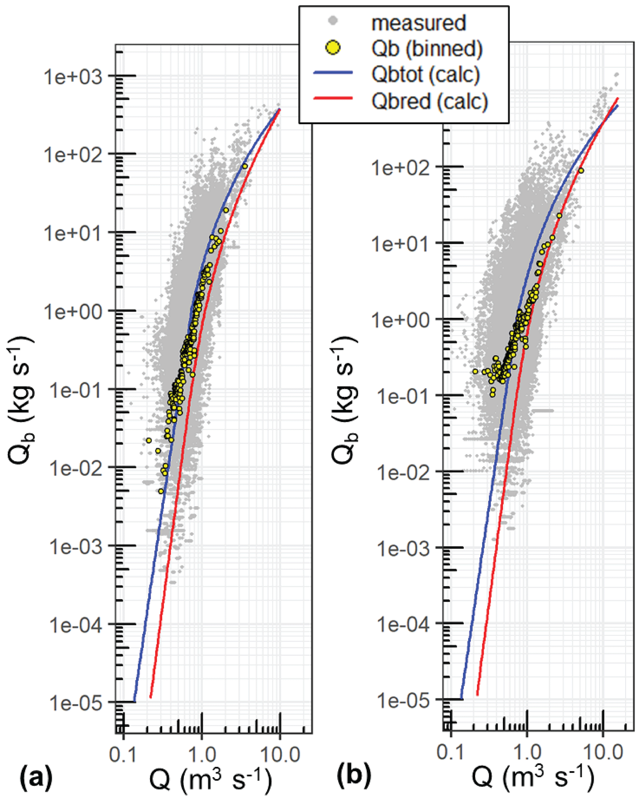
Figure 2Measurements of bedload transport Qb vs. discharge Q. Qb values are based (a) on the PBI sensors for period A (1986–1999, grey dots) and (b) on the geophone sensors for period B (2002–2016, grey dots). The binned values of Qb were calculated as the geometric mean, whereby zero values were replaced by the QbM values (see Sect. 2.6 for explanation). The red and blue lines represent the calculated bedload transport rates (described in section 2.5).
2.6 Accounting for zero bedload transport values and use of the transport disequilibrium ratio
The time series of bedload transport included the same 522 flood events as used in Rickenmann (2020, Table 1 therein). Observations of bedload transport often show a large variability for a given discharge value, typically covering several orders of magnitudes, as illustrated in Fig. 2. In such a situation, when binning the measurements in discharge classes to determine a mean trend of the observed transport rates, it is preferable to calculate a geometric mean of the Qb values. However, this brings about the problem of how to deal with observed zero Qb values. Here, I took an approach similar to that proposed by Gaeuman et al. (2009, 2015), averaging the zero Qb values with (temporally) neighbouring non-zero Qb values. I replaced the zero Qbz values by averaging any k successive zero Qbz values by including the two neighbouring non-zero Qbz_p and Qbz_a values, where the indices stand for prior to (p) and after (a) a series of k successive zero Qbz values. Then I assigned to all (k+2) values the average value QbM= (Qbz_p+Qbz_. The grey dots in Fig. 2 show the Qb=QbM values, and the binned Qb values in Fig. 2 were calculated as the geometric mean of the QbM values for any given discharge class.
For the event-based analysis of bedload transport at the Erlenbach, I had used the disequilibrium ratio Ed, calculated as , where Mgravel is the transported bedload mass per event, and Mgreg is the estimated bedload mass per event based on the calculation of Qbtot (Rickenmann, 2020). Here, I introduce a similar disequilibrium ratio EdM, which is based on the measured 1 min values QbM and on the calculated bedload transport rates Qbtot (Eq. 2). The use of QbM values has the advantage of facilitating the analysis using the full data set including all minute values.
Qbtot values were used in Eq. (2) because of a better comparability with the event-based analysis in Rickenmann (2020) and because these values better approximate the mean trend of the measured transport rates than the Qbred values (Fig. 2). One goal of the present study was to compare some general results of the analysis using the 1 min values with the event-based analysis reported in Rickenmann (2020), such as memory effects and the negative correlation between threshold discharge and disequilibrium ratio. There, it was observed that there was a memory effect for the Ed values and also for the Qs and the Qe values for a lag of at least three events for period A and somewhat longer for period B. It is also known from earlier studies that the correlation between Qb and Q increases for aggregation times up to 60 min (Rickenmann, 2018). Given a typical event duration of 60 to 90 min and that at least 85 % of the events had durations of more than 30 min (Fig. S1), the following smoothing procedure was applied to the 1 min values in order to delineate typical cycles with EdM values above and below the median for all events of a given period: (i) a kernel smoothing was applied to the QbM values with a bandwidth of 30, resulting in the Qbks30 values; (ii) smoothened EdM values were first determined as Edks30= ; (iii) then a kernel smoothing was applied to the log(Edks30) values with a bandwidth of 300, resulting in the so-called Edks values. In the first step (i), the selected bandwidth of 30 with a Gaussian kernel (used here) smoothens over a window of roughly 60 min values. This value was selected because it resulted in a smoothing of the short time fluctuations in bedload transport (with an associated increase in correlation between Qb and Q) and because the majority of the events have a longer duration. The last step (iii) represents roughly a smoothing of the Edks30 values over 3 to 5 events. The resulting spread of the log(Edks) values (−1 to 1 for period A, −1 to 2 for period B) is roughly analogous to the spread of the log(Ed) values (−0.5 to 0.5 for period A, −0.5 to 1 for period B; Rickenmann, 2020, Fig. 6 therein) for the event-based analysis, for which the log(Ed) values were smoothened with a moving average over five events, before determining the cyclic variations (Rickenmann, 2020).
2.7 Hysteresis index
Several dimensionless numbers were developed and discussed to characterise the hysteresis between hydrological variables at the discharge event timescale (Lloyd et al., 2016; Zuecco et al., 2016). The index of Lloyd et al. (2016) was developed in the context of analysing the hysteresis behaviour of suspended sediment measurements, and it was later also applied by Misset et al. (2018) and by Vale and Dymond (2019). It essentially calculates the difference in suspended sediment values on the rising and falling limbs and normalises the differences at every measurement point. This results in an index between −1 and 1 that is equal to 0 if there is no loop.
I have tested some of the approaches for the bedload transport events at the Erlenbach, comparing the index values with a visual assessment of the hysteresis direction and magnitude. I found that the index proposed by Lloyd et al. (2016) works well when applied to bedload transport intensities using logarithmic (instead of linear) values of the impulse counts (IMP) to calculate differences and normalise these. Thus, the hysteresis index HI_log was calculated as summarised in Sect. A2.
2.8 Sediment availability on the streambed
From repeated longitudinal streambed profile surveys, partly reported by Turowski et al. (2013), we estimated the cumulative erosion or deposition volume along the 550 m long Erlenbach study reach upstream of the measuring site (Rickenmann, 2020, Fig. 10 therein). Apart from the three exceptional flood events reported in Table 2, we did not observe any substantial destruction of steps in the Erlenbach since 1986 along this study reach. This agrees with local erosion or deposition reported by Turowski et al. (2013), which was mostly less than about 0.7 m along the study reach for periods excluding the three exceptional events. For such periods, the maximum of deposited or eroded sediment volumes indicated smaller changes in storage volumes than during and after the occurrence of the exceptional events. These findings were interpreted in Rickenmann (2020) together with field observations of bedload particle displacements with tagged grains in the Erlenbach reported by Schneider et al. (2014), resulting in the conclusion that the mean depth (thickness) of the active layer on the bed was approximately twice as large in period B as in period A. This indicated a generally higher sediment availability in period B than in period A. No information was available on the temporal variability in characteristic grain sizes along the study reach.
3.1 Characteristic ranges of discharges and disequilibrium ratios
The general trend of measured and calculated bedload transport rates in the Erlenbach is similar (Fig. 2). However, there is a wider spread of discharges for a given level of bedload transport in period B than in period A (Fig. 2), and for Q < 0.5 m3 s−1 the binned means of the QbM values show a different trend for period B than for period A. A more detailed analysis of the somewhat different discharge and bedload transport observations for the two periods, particularly for Q < 0.5 m3 s−1, is presented in the Supplement (Sect. S1, Figs. S2–S8). The main findings from this analysis are (i) for Q smaller than 1 m3 s−1, but particularly for Q < 0.5 m3 s−1, there were relatively more Qbz= 0 values and relatively more small QbM values in period A than in period B; (ii) contrary to expectations, for Q < 1 m3 s−1 the average Q values in period A were larger than those in period B; (iii) for Q > 1 m3 s−1, both Q and QbM values were smaller on average in period A than in period B.
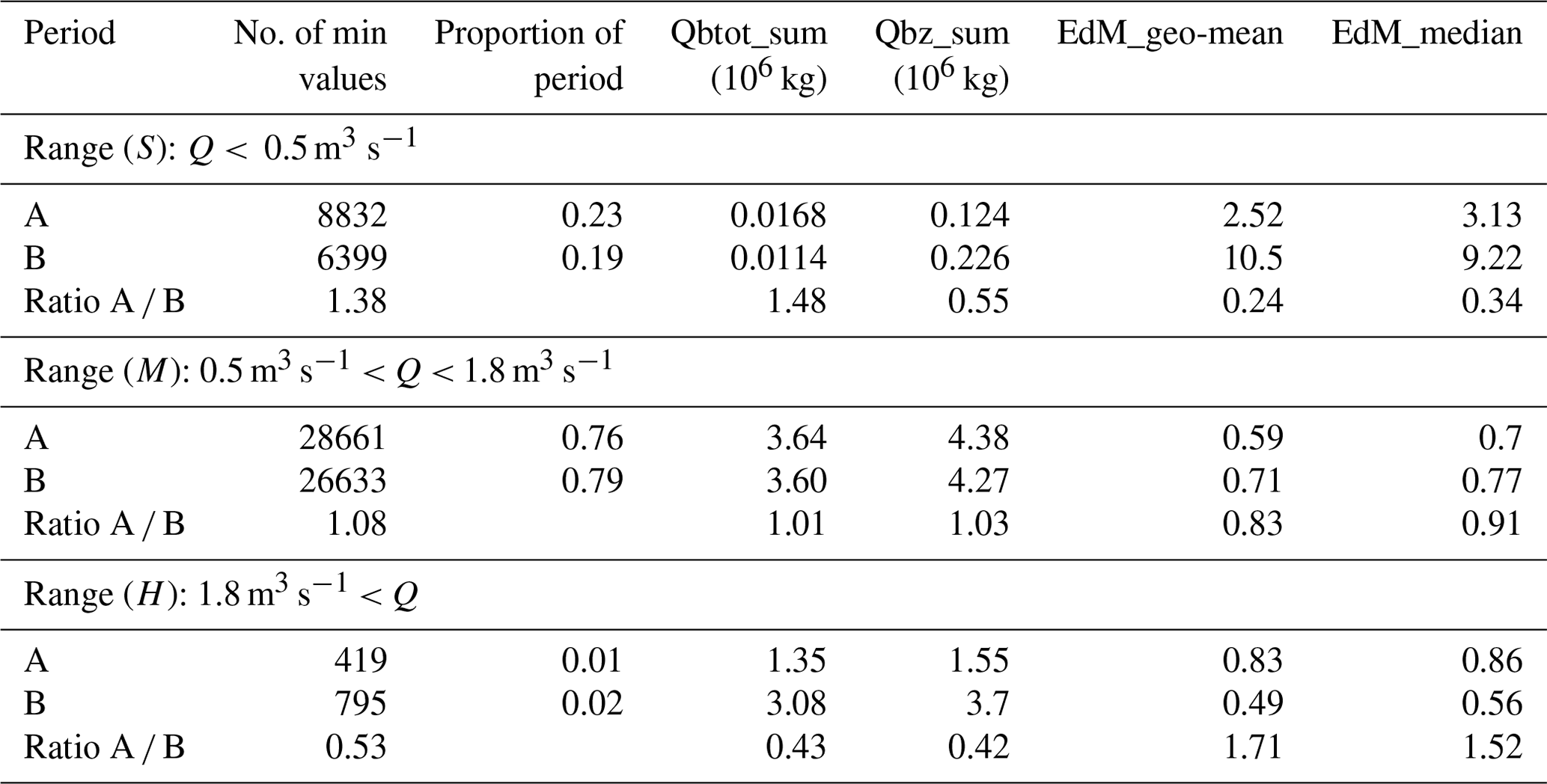
To further compare the flow and transport conditions for period A and period B, binned values over 0.1 m3 s−1 wide discharge classes were determined for three variables, as shown in Fig. 3. The measured (QbM) and calculated (Qbtot) bedload transport rates are shown as time-integrated values, by multiplying the binned means by 60 s and summing them over the number of values per bin – QbM_sum, Qbtot_sum – and for the disequilibrium ratios the mean values were determined with the logarithmic values (LEdM_mean). In Fig. 3 we can observe three characteristic discharge ranges (), and characteristic values for these three ranges are summarised in Table 1. In the domain S (small discharges, Q < 0.5 m3 s−1) there is a large deviation of the EdM values from the mean for both periods, which may be partly due to measurement uncertainties, whereas in the other domains the EdM values fluctuate around 1. The time-integrated transport in domain S (Qbz_sum values in Table 1) is negligible in relation to the total for each period. The domain M (medium discharges, 0.5 m3 s−1 < Q < 1.8 m3 s−1) is characterised by a similar bedload transport behaviour for periods A and B, with almost the same transported bedload masses in both periods, and similar binned mean of EdM values and hydraulic forcing (Qbtot_sum values in Table 1). In the domain H (high discharges, Q > 1.8 m3 s−1) we observe roughly similar flow and bedload transport characteristics for both periods for Q up to about 5 m3 s−1 (Figs. 2, 3). However, in period B there were two exceptional flood events (Table 2) with Qmax > 5 m3 s−1, whereas in period A there was only one such exceptional flood event (Table 2), with only about half the transport time duration.
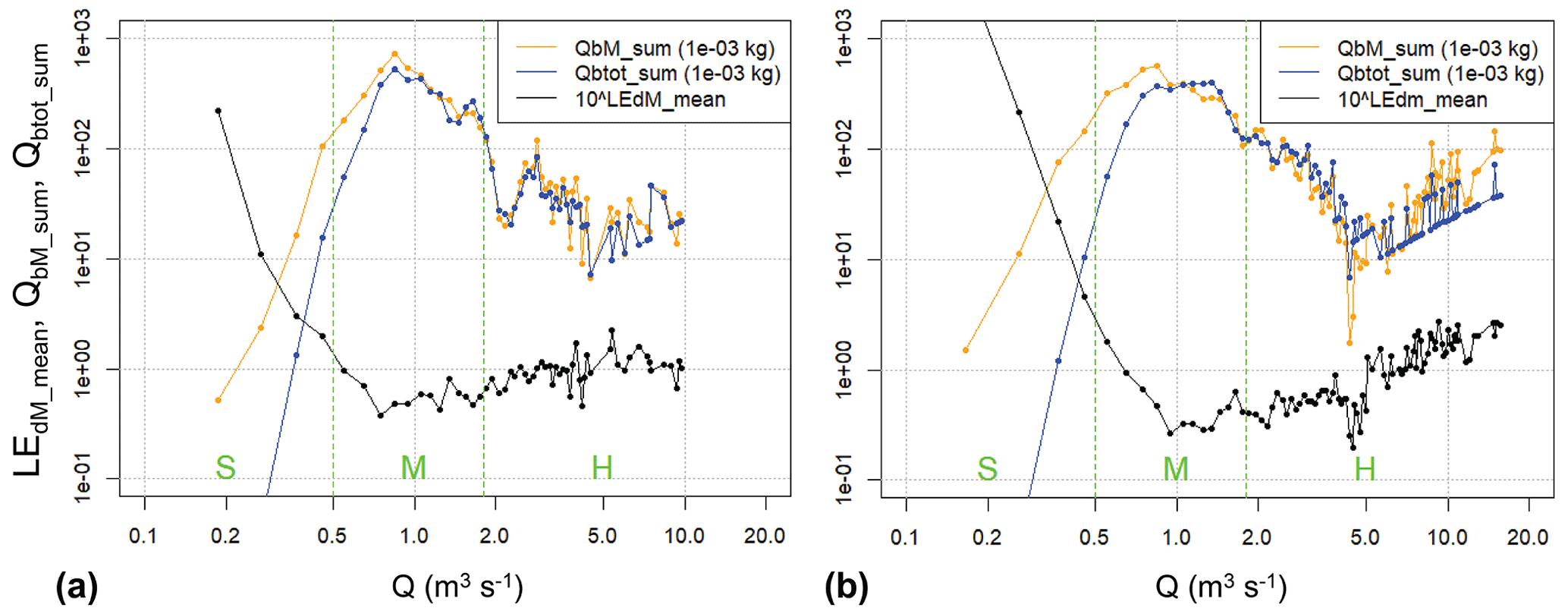
Figure 3Binned values over 0.1 m3 s−1 wide discharge classes are shown for the measured (QbM) and calculated (Qbtot) bedload transport rates as time-integrated values (QbM_sum and Qbtot_sum) and for the logarithmic means of the disequilibrium ratios (LEdM_mean), separately for (a) period A and (b) period B. The vertical dashed green lines separate the three characteristic ranges () of discharge (see text for more details).
The roughly parallel lines of QbM_sum and Qbtot_sum in Fig. 3 indicate that there is a certain correlation between the measured bedload transport and the driving force discharge (expressed in terms of calculated transport). To assess how the correlation between flow and transport increases with integration time, the Pearson correlation coefficient R was determined between log(QbM) and log(Qbtot) (Fig. 4). This calculation was done separately for periods A and B, but also for subsets including sub-periods with only above- (“high”, EDH) and below-median (“low”, EDL) Edks conditions, respectively. This analysis resulted in two important differences: correlation is larger in both periods for EDH conditions than for EDL conditions, and correlation is larger in period A than in period B.
Table 1Characteristic bedload transport values determined for the three characteristic discharge ranges (), as delineated in Fig. 3.
The logarithmic values of the smoothened disequilibrium ratios (Edks) are shown over time (no. of minute time steps) for both periods in Fig. 5. In this figure a cyclic fluctuation in the Edks values can be observed, similarly to what had been found previously for the event-based analysis of the disequilibrium ratio for the same observation periods in the Erlenbach (Rickenmann, 2020). The cyclic fluctuations in Edks in Fig. 5 were used as a basis to delineate sub-periods (p1–p13) with primarily EDH or EDL conditions based on a visual assessment, and the exact limits were determined in such a way that they were identical to flood event limits. This resulted in seven sub-periods for period A and in six sub-periods for period B, respecting as a further criterion that all these sub-periods should include a similar number (within a factor of about 2) of 1 min time steps (Table 2).
Table 2Identified sub-periods (see also Fig. 5) and their main characteristics in terms of number of minute values, number of flood events, mean EdM level, peak flow (Qmax) of the most important flood per sub-period, and the dates of the three exceptional flood events. a The geometric mean of the 1 min EdM values is also given, as compared to b the geometric mean of the seven (period A) and six (period B) mean values per sub-period given in this table.
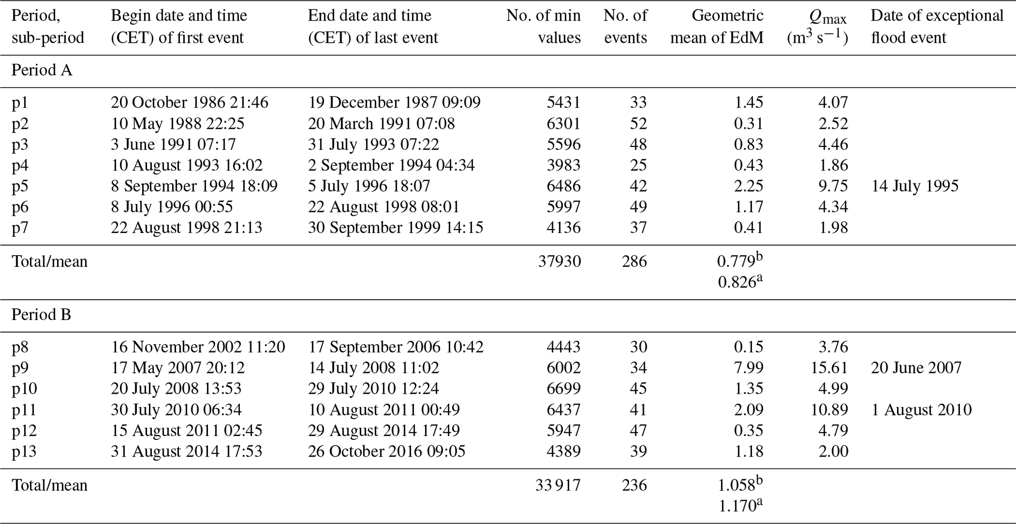
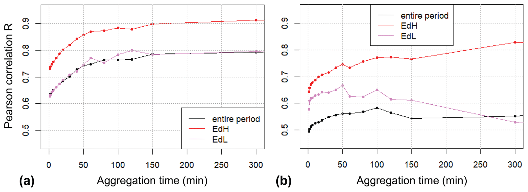
Figure 4Pearson correlation R between log(QbM) and log(Qbtot) as a function of aggregation time for (a) period A and (b) period B. EDH and EDL refer to sub-periods with above- (“EDH, high”) and below-median (“EDL, low”) Edks conditions, respectively.
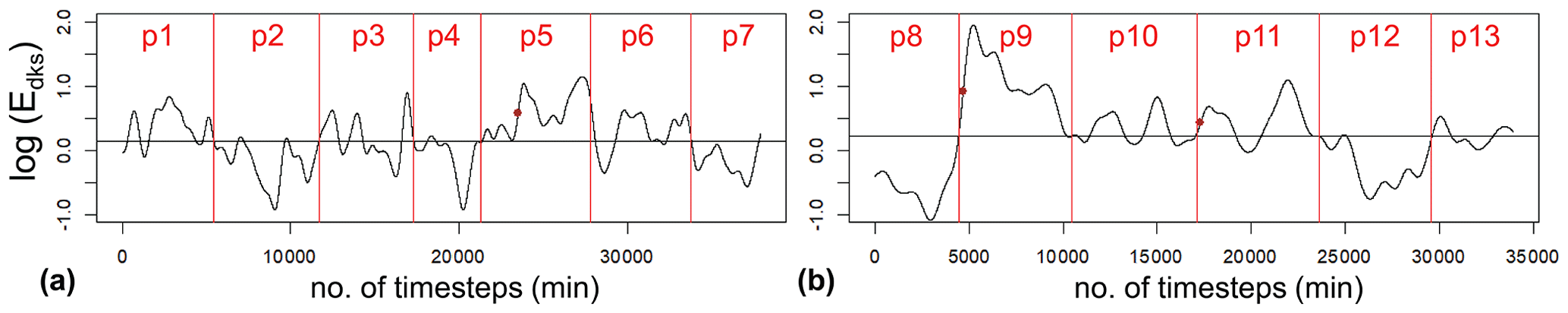
Figure 5Smoothened disequilibrium ratio (Edks) as a function of the number (no.) of time steps for (a) period A and (b) period B. The vertical red lines delineate sub-periods for which the limits are identical to event limits. The red dots refer to the three exceptional flood events. The horizontal black line indicates the median Edks value for period A and B, respectively.
The generally stronger correlation between log(QbM) and log(Qbtot) in period A than in period B (Fig. 4) may be partly due to a wider spread of discharges for a given level of bedload transport in period B than in period A (Fig. 2). The wider spread of discharges and the more horizontal distribution of binned QbM values for Q < 0.5 m3 s−1 (Fig. 2) may reflect a wider range of phase 1 transport conditions (whereby transport rates are relatively low until a certain flow level is reached; Ryan et al., 2002) for period B than for period A, as indicated by the smoothened trend lines for QbM versus Q that were determined separately for each sub-period of Table 2 (Fig. S9). The observation of a stronger correlation between log(QbM) and log(Qbtot) for EDH conditions than for EDL conditions (Fig. 4) may be partly due to the fact that there were relatively fewer Qbz= 0 values for EDH conditions than for EDL conditions, as is indicated in Table 3.
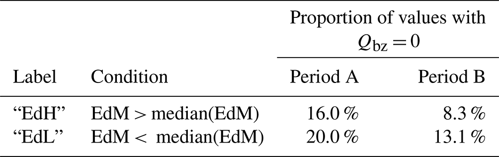
Table 3Separation of all bedload transport observations into two subsets of equal number of observations per (main) period, with either above- (“high”, EDH) or below-median (“low”, EDL) EdM conditions. For these subsets, the table indicates the proportion of values with Qbz= 0, i.e. the percentage of values when zero bedload transport was measured during 1 min intervals of the transport events.
3.2 Autocorrelation coefficient of bedload transport rates as a function of lag time
Given a median flood event duration of about 95 to 100 min for both periods (Fig. S1), I determined the autocorrelation coefficient (ACF) of log(QbM) and of log(EdM) for lag times up to 100 min separately for periods A and B (Fig. 6). The main findings of this analysis are that the ACF values of log(QbM) are roughly similar for both periods for lag times up to about 50 min (Fig. 6a, b) and that in period B the two sub-periods with the two exceptional flood events (p9, p11) have among the largest ACF values. Regarding the ACF values of log(EdM), they are clearly larger for period B than for period A (Fig. 6c, d), and in both main periods the sub-periods with the largest exceptional flood events (p5, p9, p11) have among the largest ACF values for lag times up to 100 min.
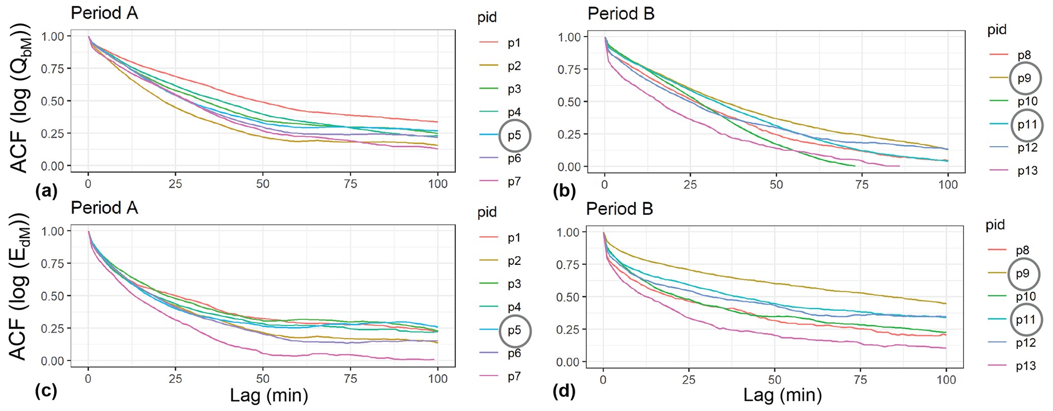
Figure 6Autocorrelation coefficient (ACF) of log(QbM) (a, b) and ACF of log(EdM) (c, d) for the main sub-periods indicated in Fig. 5; “pid” refers to the identification of the sub-period. The grey circles indicate inclusion of one of the three exceptional flood events.
A correlation matrix was determined for seven variables for the 13 sub-periods in Table 2 (Fig. 7a), namely the mean ACF values over lag times up to 30 min for the log values of Qbtot, QbM, and EdM (ACF_LQbt_m30, ACF_LQbM_m30, ACF_LEdM_m30); the mean of the log values of Qbtot, QbM, and EdM (LQbtot_mean, LQbM_mean, LEdM_mean); and the mean of the linear values of QbM (QbM_mean). The 30 min time frame was selected because there is a relatively strong increase for an aggregation time up to 30 min in the correlation between Qb and Q (Fig. 4) and because most event durations are clearly longer than 30 min (Fig. S1). The strongest correlation for the mean ACF values was found between ACF_LEdM_30 and QbM_mean, which is graphically illustrated in Fig. 7b. There the two sub-periods with the two largest exceptional flood events (p9, p11) contribute much to the strong correlation, although the data from the other sub-periods support the general trend line.
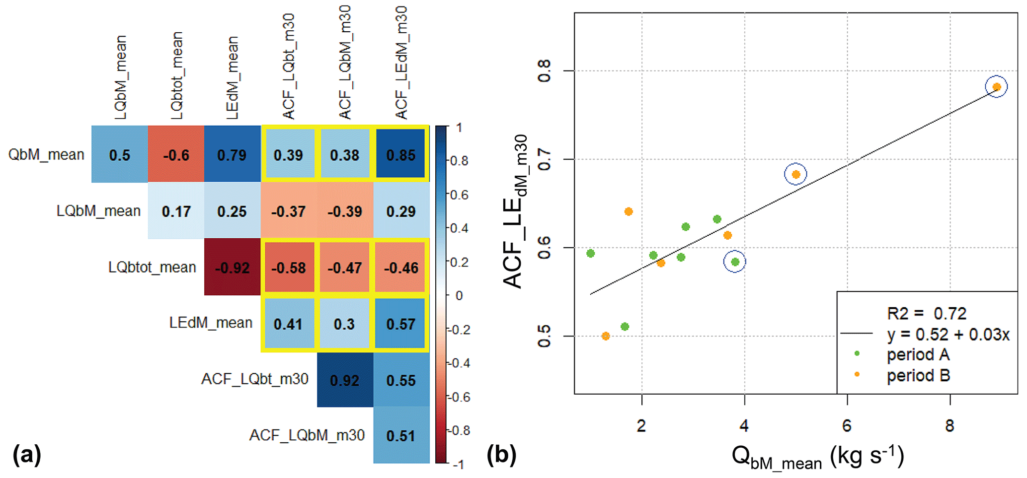
Figure 7(a) Correlation matrix with Pearson correlation coefficient R for seven variables determined for all the 13 sub-periods indicated in Fig. 5 and Table 2. The fields with a yellow box indicate those variable combinations with a reasonably strong correlation for which the correlation has the same sign (positive or negative) also when considering only period A and period B separately (see Fig. S10). (b) Mean autocorrelation coefficient of log(EdM) over the first 30 lag minutes (ACF_LEdM_m30) vs. linear mean of QbM values (QbM_mean), determined for each of the 13 sub-periods. The blue circles around a point indicate the inclusion of one of the three exceptional flood events.
The fields with a yellow box in the correlation matrix of Fig. 7a indicate those variable combinations with a reasonably strong correlation, for which the correlation has the same sign (positive or negative) also when considering only period A and period B separately (Fig. S10). However, the correlation between the log values of EdM (ACF_LEdM_m30) and the log values of QbM (LQbM_mean) is clearly weaker than for the case of using linear values of QbM (QbM_mean) (Fig. 7a). In addition, the sign of the correlation between ACF_LQbt_m30 and LQbM_mean is different for period A and B (Fig. S10). This is an indication that only larger transport events (that dominate the linear averaging) clearly increase autocorrelation and thus memory effects.
3.3 Critical discharge at the start and at the end of a transport event
For the 13 sub-periods (Table 2), the means of both the critical discharge at the start and at the end of a transport event show a fairly strong correlation with the geometric means of the EdM values (Fig. 8). For comparison, it is noted that for the event-based analysis in Rickenmann (2020) the squared correlation coefficient between Qe and Ed is R2= 0.26, and between Qs and Ed it is R2= 0.20. These R2 values are clearly lower than those given in Fig. 8. The analysis based on the 13 sub-periods represents on average an aggregation time 40 times longer than for the event-based analysis (the factor of 40 is determined as the ratio of 522 events over 13 sub-periods). Similarly, there is a fairly strong correlation between the means of both the critical discharge at the start and at the end of a transport event and the geometric means of Qbtot (Fig. 9).
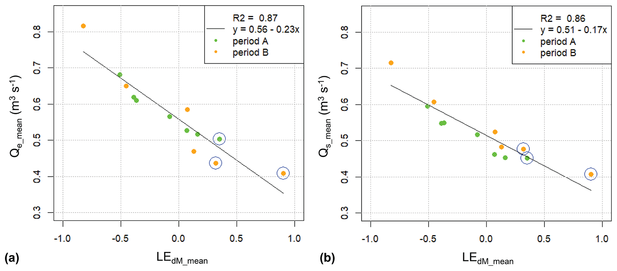
Figure 8Correlation between variables determined for each of the 13 sub-periods. (a) Mean discharge threshold at the end of an event Qe (Qe_mean) vs. the geometric mean of the disequilibrium ratio EdM (LEdM_mean). (b) Mean discharge threshold at the start of an event Qs (Qs_mean) vs. the geometric mean of the disequilibrium ratio EdM (LEdM_mean). The blue circles around a point indicate inclusion of one of the three exceptional flood events.
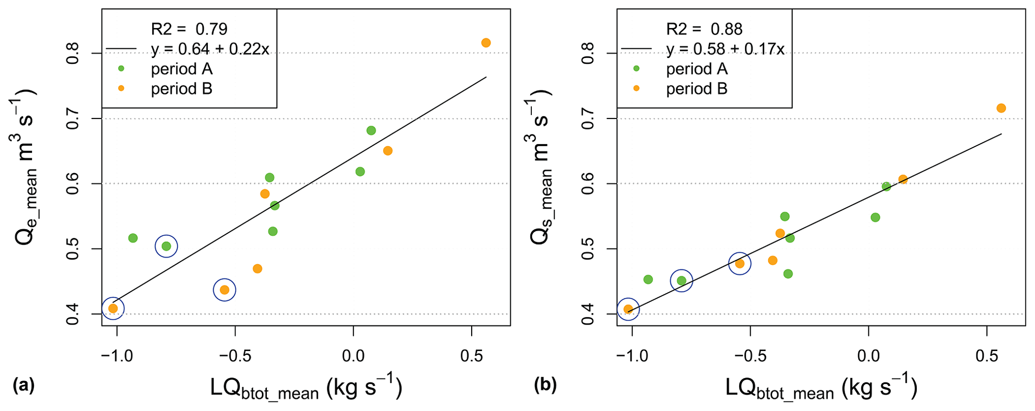
Figure 9Correlation between variables determined for each of the 13 sub-periods. (a) Mean discharge threshold at the end of an event Qe (Qe_mean) vs. the geometric mean of the calculated transport rate Qbtot (LQbt_mean). (b) Mean discharge threshold at the start of an event Qs (Qs_mean) vs. the geometric mean of the calculated transport rate Qbtot (LQbt_mean). The blue circles around a point indicate inclusion of one of the three exceptional flood events.
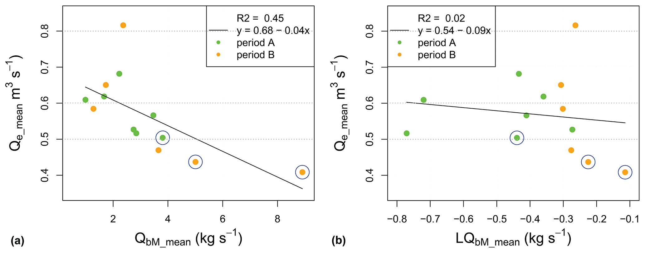
Figure 10Correlation between variables determined for each of the 13 sub-periods. (a) Mean discharge threshold at the end of an event Qe (Qe_mean) vs. the linear mean of the bedload transport rate QbM (QbM_mean). (b) Mean discharge threshold at the end of an event Qe (Qe_mean) vs. the geometric mean of the bedload transport rate QbM (LQbM_mean). The blue circles around a point indicate inclusion of one of the three exceptional flood events.
If we consider the correlation between Qe and QbM in Fig. 10a, it is clearly lower than the correlations of Qe with log(EdM) and log(Qbtot) in Figs. 8 and 9, respectively. Calculating the mean values per sub-period with the geometric instead of the linear mean of the QbM values results in a vanishing correlation between the two variables (Fig. 10b). These findings are consistent with the event-based analysis in Rickenmann (2020).
3.4 Coefficient of variation of the bedload transport rates
Since the discharge Q (or hydraulic forcing) is the primary control on bedload transport rates, the coefficient of variation (cv) of the bedload transport rates QbM (cv_QbM) was determined for Q-ordered values. Each bin had a constant width of approximately 200 values, and both cv_QbM and the linear mean of the bedload transport rates QbM (QbM_mean) were calculated. The cv values were determined for the following two cases: (i) period A and period B were considered separately, and (ii) for both periods A and B combined, the data were divided into one group pertaining to the rising limb and a second pertaining to the falling limb of the hydrograph (denoted as HR and HF, respectively) of each flood event, taking the maximum discharge of an event to separate the two limbs. A theoretically more correct calculation of cv values was also made with Qbz instead of QbM values. This resulted in very slightly increased cv values, mainly for period A at small discharges, with more Qbz= 0 values in period A than in period B. For the sake of simplicity, the cv_QbM values are presented here, since all the other analyses were made and presented with QbM values.
For case (i) cv_QbM values vary essentially between about 1 and 3. In terms of discharge, three ranges can be distinguished. For both 0.4 m3 s−1 < Q_mean < 0.6 m3 s−1 and for 0.9 m3 s−1 < Q_mean < 1.6 m3 s−1 the cv values are significantly smaller for period A than for period B (Fig. 11a, c), whereas cv values are not significantly different between the two periods for an intermediate discharge range 0.6 m3 s−1 < Q_mean < 0.9 m3 s−1 (Fig. 11b). For the lowest discharge range, the larger cv values for period B are associated with significantly larger bedload transport rates in period B than in period A (Fig. 12a). In the other (higher) two discharge ranges there is no significant difference in the bedload transport rates (Fig. 12b, c).
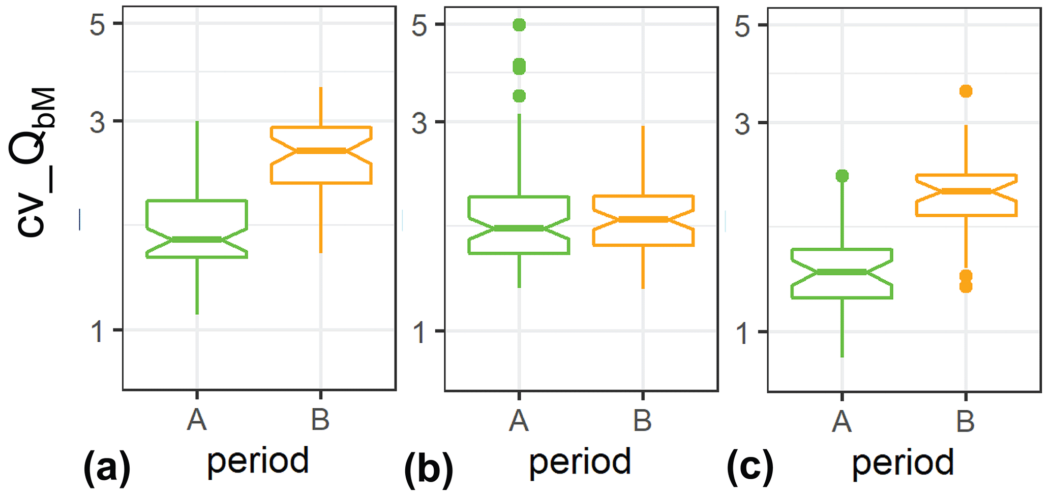
Figure 11Boxplots of the coefficient of variation of bedload transport rates (cv_QbM) determined for binned Q values, each containing 200 values, shown for different discharge ranges: (a) 0.4 m3 s−1 < Q_mean < 0.6 m3 s−1, (b) 0.6 m3 s−1 < Q_mean < 0.9 m3 s−1, (c) 0.9 m3 s−1 < Q_mean < 6 m3 s−1.
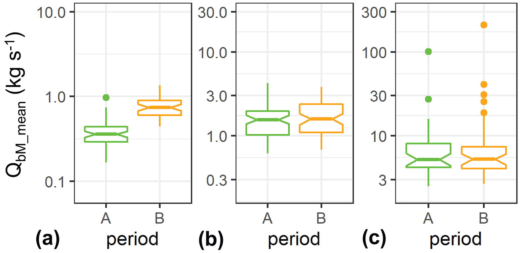
Figure 12Boxplots of the linear mean of bedload transport rate (QbM_mean) determined for binned Q values, each containing 200 values, shown for different discharge ranges: (a) 0.4 m3 s−1 < Q_mean < 0.6 m3 s−1, (b) 0.6 m3 s−1 < Q_mean < 0.9 m3 s−1, (c) 0.9 m3 s−1 < Q_mean < 6 m3 s−1. Note different ordinate values but similar scaling to allow an easy visual comparison of the spread of the values in the different discharge ranges.
For case (ii) using the groups of HR and HF values, cv_QbM values are significantly smaller on average for the rising limb (HR) than for the falling limb (HF) flow conditions, whereby the relative difference is more pronounced for discharges Q_mean > 1 m3 s−1 than for Q_mean < 1 m3 s−1 (Fig. 13a, b). For increasing discharges larger than about 0.5 m3 s−1, the cv values tend to decrease (Fig. S11). Furthermore, for a discharge range of about 0.5 m3 s−1 < Q_mean < 1.8 m3 s−1, a predominant clockwise hysteresis behaviour appears to be most pronounced, as reflected by generally larger average QbM values for the rising than for the falling limb (Fig. 13c).
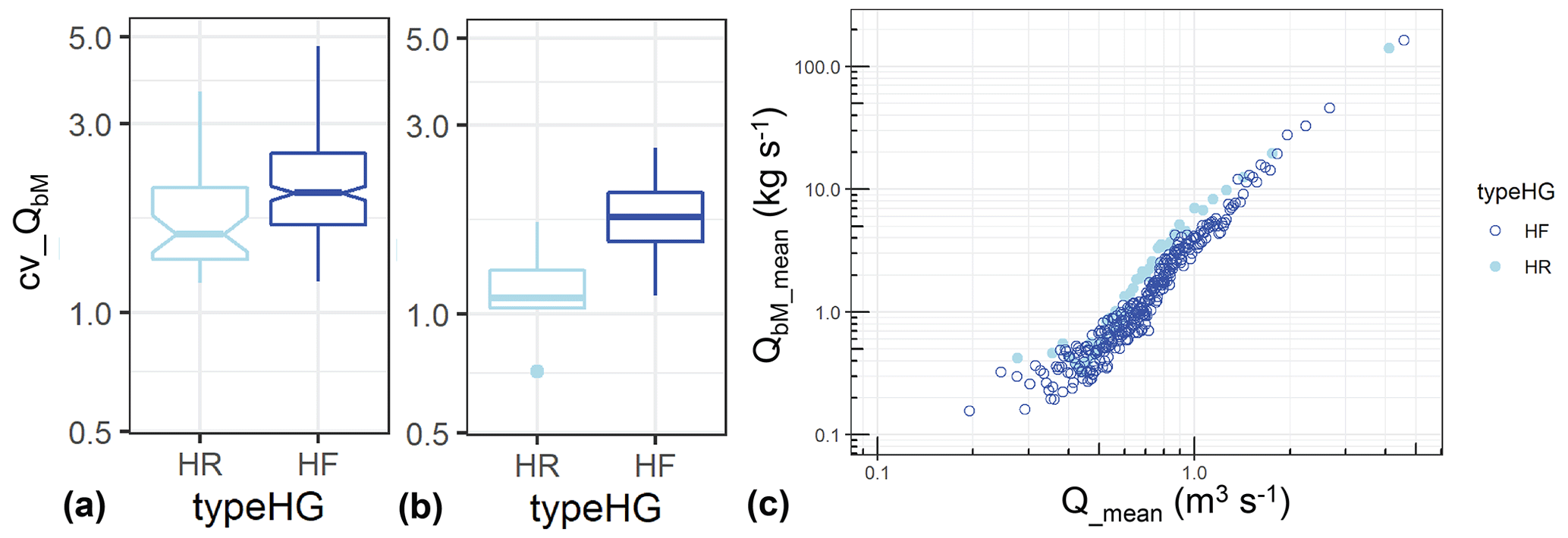
Figure 13Boxplots of the coefficient of variation of bedload transport rates (cv_QbM) for the rising part (HR) and the falling part (HF) of the hydrograph, shown in (a) for smaller discharges Q_mean < 1 m3 s−1 and in (b) for larger discharges Q_mean > 1 m3 s−1. (c) Linear mean of bedload transport rates (QbM_mean) vs. linear mean of discharge (Q_mean), determined separately for HR and HF conditions.
3.5 Hysteresis index
The hysteresis index HI_log generally varies between −0.5 and 0.75 for both periods A and B (Fig. 14). For increasing Qmax values, a decrease in the spread of the HI_log values is observed in the range of discharges of about 1 m3 s−1 < Qmax < 2 m3 s−1 (Fig. 14a). A similar decrease in the spread of the HI_log values occurs in the range of event bedload masses (Mgravel) of about 1×10⁴ kg < Mgravel < 1×10⁵ kg (Fig. 14b). It is further observed that the HI_log values for period B are significantly smaller on average than for period A (Fig. S12), with the HI_log values changing somewhat for different discharge ranges (; see Fig. 3). In the high discharge range (Q > 1.8 m3 s−1), the values indicate less clockwise behaviour, and the difference between period A and B is largest (Fig. S12c). The hysteresis analysis clearly shows a dominant clockwise hysteresis pattern in the Erlenbach stream, and the largest HI_log values are generally observed in the intermediate discharge range 0.5 m3 s−1 < Q_mean < 1.8 m3 s−1 (Figs. 14, 13c, S12).
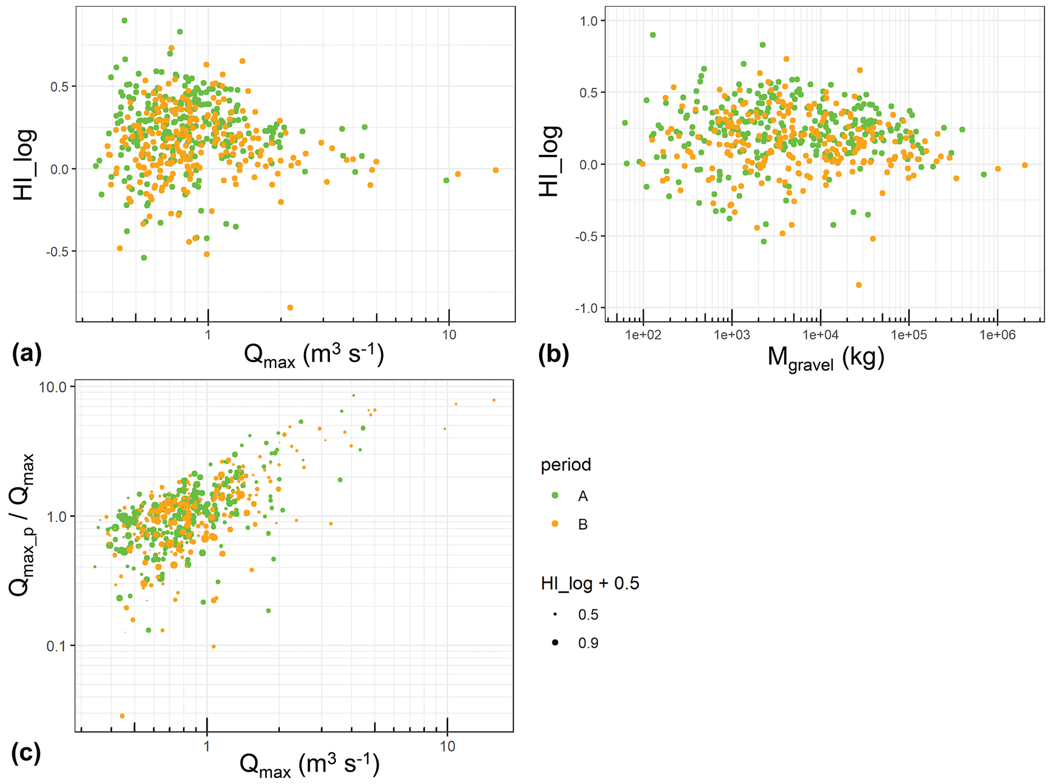
Figure 14(a) Hysteresis index HI_log vs. maximum discharge Qmax of an event. (b) Hysteresis index HI_log vs. total transported bedload mass of an event (Mgravel). (c) Effect of normalised maximum discharge of the preceding flood event ( shown vs. Qmax, with the degree of hysteresis (HI_log) indicated by the data point size; larger circle sizes indicate a stronger clockwise hysteresis.
The lower limit for the start of the decreasing spread of HI_log values (Fig. 14b), Mgravel= 1×10⁴ kg, corresponds to a bulk bedload volume (including porosity) of about 7.4 m3. For the lowermost natural reach with bw= 4.1 m and a length of about 50 m, this roughly corresponds to a mean thickness hm of a (mobile) bedload layer stored in this reach of about hm= 7.4 m3/205 m2= 0.04 m. The upper limit of the decreasing spread of HI_log values (Fig. 14b), Mgravel= 1 105 kg, is equivalent to a bulk bedload volume (including porosity) of about 74 m3, corresponding to a mean thickness hm of about 0.36 m. These two values for hm are of the order of the D50 and the D84 of the surface bed material, respectively.
A possible effect of channel destabilisation on the hysteresis behaviour is shown in Fig. 14c. The normalised maximum discharge of the preceding flood event (Qmax_p) Qmax is shown to influence the degree of hysteresis (HI_log value) in that for values of about (Qmax_p) Qmax > 1.5 and Qmax > 1.3 m3 s−1, there are very few events with a strong clockwise hysteresis (HI_log > 0.4, i.e. HI_log +0.5 > 0.9). This implies that antecedent large-magnitude floods tended to result in less clockwise hysteresis in the following flood event with a minimum size of Qmax > 1.3 m3 s−1.
It may be mentioned that there is some similarity of the analyses presented in this study, i.e. mainly the results presented in Figs. 6 to 10, to the earlier study of Rickenmann (2020). However, in the earlier study all flood events had the same weight in the analysis (independent of the event duration), whereas in this study each single observation on bedload transport (i.e. 1 min value) had the same weight. All the other results are completely new and could not have been obtained using the event-based analysis presented in Rickenmann (2020). In the first part of this study the minute-based analysis examined longer time intervals than the event-based analysis, whereas in the second part of this study, the minute-based analysis considered shorter time intervals than the event-based analysis and also examined variations in the coefficient of variation of the transport rate and hysteresis effects.
4.1 Averaging and characteristic trends
In some parts of the analysis, different trends were found for transport conditions that imply either above-average disequilibrium ratios or below-average disequilibrium ratios. These conditions are identified as time steps with above- (“high”, EDH) and below-median (“low”, EDL) Edks values, respectively. The event-based analysis of the Erlenbach sediment transport data had indicated that EDH conditions are likely associated with a larger sediment availability on the streambed than EDL conditions; in addition, clearly larger disequilibrium ratios were observed in period B than in period A, associated with a larger volume of sediment stored on the streambed (Rickenmann, 2020). In previous studies, the correlation between hydraulic forcing and bedload transport rate has been shown to increase with increasing aggregation time (e.g. Lenzi et al., 2004; Recking et al., 2012; Rickenmann, 1994, 2018; Rickenmann and McArdell, 2008). This is confirmed for the Erlenbach when considering maximum aggregation times of 300 min (with most flood events not exceeding 300 min in duration; Fig. S1), for which the correlation coefficients R also increase with increasing aggregation time (Fig. 4). The analysis of the Erlenbach data further shows that the correlation between the two variables is larger for above-average bedload transport (EDH) than for below-average bedload transport (EDL) (Fig. 4). This statement appears to contradict the fact that R values are generally smaller for period B than for period A (Fig. 4) because larger volumes of sediment stored on the streambed were observed in period B than in period A (Rickenmann, 2020). However, the smaller R values for period B than for period A may be due to the more frequent occurrence of widely varying bedload transport rates for small discharges during period B (Fig. 2). This is associated with more pronounced phase 1 transport conditions (Ryan et al., 2002) in period B than in period A (Fig. S9; for Q values smaller than about 0.5 m3 s−1), including larger fluctuations in Q and Qb without a clear correlation between the two variables.
In the event-based analysis of Erlenbach bedload transport measurements, the threshold discharge for transport (Qs, Qe) was found to correlate positively with hydraulic forcing (Qbtot) and negatively with the disequilibrium ratio (EdM) (Rickenmann, 2020). This finding is confirmed by the present analysis for the 13 sub-periods (Table 2, Fig. 5), for which the aggregation times were about 40 times longer than for the event-based analysis, resulting in correlation coefficients R2 between Qs or Qe and Qbtot or EdM ranging from 0.88 to 0.79 (Figs. 8 and 9), compared to correlation coefficients R2 of up to 0.26 for the event-based analysis (Rickenmann, 2020). If we consider the correlation between Qs or Qe and transport rate QbM, the R values for a (negative) correlation were smaller than between Qs or Qe and Qbtot or EdM: for the event-based analysis a correlation was found only for those events with a peak discharge Qmax larger than 1 m3 s−1 (Rickenmann, 2020), and for the new analysis a correlation was found only when determining linear mean values of QbM for each sub-period (Fig. 10). This finding suggests that only flow conditions with more important bedload transport activity can influence the threshold transport conditions.
In contrast to the event-based analysis (Rickenmann, 2020), the sub-periods defined in Fig. 5 may suggest longer full-cycle durations. For period A, one could infer two full cycles (taking sub-periods p5 and p6 together), resulting in cycle duration of about 6.5 years (as compared to 0.9 years for the event-based analysis). For period B, one could infer one very long cycle of about 10 years (sub-periods p8 to p11) and one of 4 years (as compared to 1.6 years for the event-based analysis). However, the delineation of the sub-periods in this study was made to explore the effect of an averaging over aggregation periods longer than an event and not to examine the cycle durations.
The autocorrelation coefficients ACF for the 13 sub-periods for lag times up to about 30 to 50 min are generally comparable for log(QbM) for both periods A and B and for log(EdM) for period B, whereas these ACF values are somewhat smaller for log(EdM) for period A (Fig. 6). For the examined ACF values, the strongest correlation is found between ACF values averaged over lag times of up to 30 min for the disequilibrium ratio (ACF_LEdM_m30) and the linear means of QbM for each sub-period (Fig. 7b). Again, the correlation is clearly stronger when using the linear mean of QbM values instead of the geometric (log) mean of QbM values (Fig. 7a). This part of the analysis indicates that the memory effect for the disequilibrium ratio increases for periods with greater bedload transport activity, a finding in agreement with the event-based analysis of the Erlenbach sediment transport data (Rickenmann, 2020) and with a flume study by Elgueta-Astaburuaga et al. (2018). Autocorrelation values of log(EdM) are generally larger for periods with increased sediment availability (period B compared to A and for sub-periods including extreme events; Fig. 6). These observations are in line with the positive correlation between ACF_LEdM_m30 and the linear means of QbM values (Fig. 7b). Autocorrelation of bedload transport rates within a time window of 30 min in this study is likely partly associated with collective entrainment of particles (e.g. Ancey, 2020a; Ma et al., 2014), as compared to completely random fluctuations that would reflect white noise behaviour without autocorrelation.
4.2 The role of sediment availability, hydraulic forcing, and bedload transport intensity in bedload transport fluctuations
For discharges Q smaller than about 0.6 m3 s−1 the cv_QbM values were smaller in period A than in period B (Fig. 11a), and the mean bedload transport rates QbM_mean were also smaller in period A than in period B (Fig. 12a). This is likely due to a higher sediment availability on the streambed in period B than in period A (Rickenmann, 2020), with more frequent phase 1 transport conditions in period B (Fig. S9) and with a more frequent occurrence of zero transport values in period A than in period B (Table 3). Phase 1 transport conditions were observed in several studies of mountain streams (Jackson and Beschta, 1982; Warburton, 1992; Ryan et al., 2002; Bathurst, 2007; Rickenmann, 2018), likely because more in-channel material was available for bedload transport.
In an intermediate range of discharges, roughly for 0.6 m3 s−1 < Qmean < 0.9 m3 s−1, which corresponds to about 0.25 kg s−1 < QbM < 2.5 kg s−1 (Fig. 2, Eq. A7), there is no clear difference in both the cv_QbM values and the QbM_mean values between periods A and B (Figs. 11b, 12b). This suggests that the generally higher sediment availability on the streambed in period B than in period A did not substantially affect the bedload transport fluctuations in this discharge range.
For discharges larger than 0.9 m3 s−1, the cv_QbM values were smaller in period A than in period B (Fig. 11c), whereas the mean bedload transport rates QbM_mean were similar in period A and in period B (Fig. 12c). It is hypothesised that for these discharge conditions, the higher sediment availability on the streambed in period B than in period A (Rickenmann, 2020) resulted in more transport fluctuations, assuming that more larger, movable particles were available on the streambed in period B, but their number on the bed was still too limited to result in a more continuous (approximately regular) high-intensity transport.
The cv values determined for the Erlenbach are partly similar to those derived from the flume and field studies cited in the Introduction of this paper but also include relatively frequent values of up to about 3. For the Erlenbach, the cv values averaged over both periods A and B tended to decrease with increasing bedload transport rates only for larger flow intensities in period A (Fig. 11c). This is qualitatively consistent with trends observed in flume studies by Kuhnle and Southard (1988) and Mettra (2014) and in a field study by Kuhnle and Willis (1998).
At the Erlenbach, smaller cv_QbM values were observed for the rising limb than for the falling limb of the hydrograph (Fig. 13a, b). The mean relative duration of the rising limb is 12.7 % of the total duration of a transporting flood event. Therefore, it is hypothesised that during this relatively short time span the available sediment on the streambed was unlikely to be quickly exhausted, in contrast to the much longer relative duration of the falling limb of 87.3 % of the total hydrograph duration. As a result, smaller cv_QbM values can be expected for the HR than for the HF conditions.
4.3 Critical discharge and sediment availability to change the transport conditions
For larger discharges and more bedload transport, the strength of the (dominant) clockwise hysteresis in the Erlenbach was reduced (Figs. 14, S12). For period B and for Q > 1.8 m3 s−1 the median hysteresis index HI_log was close to zero (i.e. no hysteresis effect), and the spread of the HI_log values was reduced. According to Fig. 14b and Sect. 3.4 there is a threshold (transported) bedload volume of about 7.4 to 74 m3, above which (clockwise) hysteresis effects tended to decrease. For the lowermost 50 m long natural reach, these volumes correspond to a mean thickness of about 0.04 to 0.36 m of stored sediment on the bed, which is of the order of the estimated thickness of the mobile bedload layer in period A (D50 to D84; Rickenmann, 2020). This is taken as indirect support for the hypothesis that, given a sufficient sediment availability on the streambed for a given hydraulic forcing (Q > 1.8 m3 s−1) to move the grains in this size range, the bedload transport hysteresis in the Erlenbach should tend to disappear, assuming that higher-flow-intensity events increase sediment availability by bank erosion and beginning step destruction (Golly et al., 2017). A partial confirmation of this idea is also based on bedload transport measurements with a moving basket downstream of the 50 m reach, which indicate that for discharges of up to 1.1 m3 s−1 no particles were transported with D > 0.2 m.
Clockwise hysteresis has been associated with a gradual decrease in sediment availability or early exhaustion of sediment sources (Pretzlav et al., 2020; Mao et al., 2019; Rovira and Batalla 2006; Gao and Pasternack, 2007). This explanation is in qualitative agreement with our observations at the Erlenbach, where less clockwise hysteresis was observed for period B than for period A (Figs. 14, S12) and where sediment availability was found to be larger in period B than in period A (Rickenmann, 2020). That lower sediment availability results in a more pronounced clockwise hysteresis, is indirectly confirmed in the Erlenbach by a trend (although weak) that increasing HI_log values tended to be associated with increasing Qe values (Fig. S13), which were found to reflect a limited sediment availability on the bed. This finding agrees with flume experiments of Mettra (2014), according to which a lower sediment supply, higher channel slope, and lower Shields stress lead to more intense hysteretic effects. Furthermore, from a review of hysteresis behaviour of sediment transport rates in alluvial streams, Gunsolus and Binns (2018) concluded that lower-magnitude hydrographs result in more pronounced hysteresis of sediment transport rates than larger-magnitude hydrographs. This finding also agrees with the observations at the Erlenbach (Figs. 14, S12).
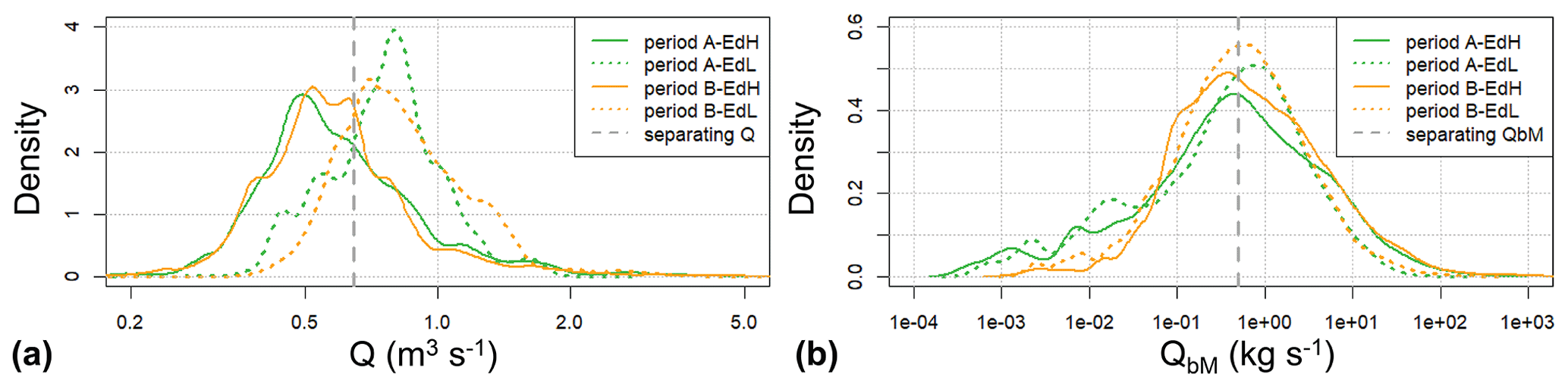
Figure 15Density distribution of two variables for EDH and EDL conditions for both periods A and B. (a) Density of Q values and (b) density of QbM values. The vertical dashed red line indicates a separating value of Q= ca. 0.645 m3 s−1 (visually determined), above which EDL conditions and below which EDH conditions dominate. A corresponding separating value is QbM= ca. 0.50 kg s−1 (determined as the mean of the median of the two periods).
Previous studies for the Erlenbach indicate that bed strengthening by low flows or low- to medium-intensity sediment-transporting flows may be important for discharges up to about 1.4 m3 s−1 (Masteller et al., 2019; Rickenmann, 2020). This tendency is supported here by the increasing threshold discharges at the start and end of an event for increasing discharge intensities (Fig. 9). For larger discharges and for exceptional floods in the Erlenbach the mobility of streambed material appears to increase, as indicated by the decreasing threshold discharges for increasing bedload transport levels and particularly including the exceptional flood events (Fig. 10). This latter observation is also supported by previous studies for the Erlenbach: step migration was observed for discharges of 4 to 5 m3 s−1 Golly et al. (2017), and substantial destruction of steps was estimated to occur at a discharge of about 7 to 10 m3 s−1 (Turowski et al., 2009, 2013). In the Rio Cordon torrent, a similar step-pool stream in northern Italy, bedload transport rates had increased by about a factor of 5 following an exceptional flood event with a peak discharge of about 10 m3 s−1 (Lenzi et al., 2004; Rainato et al., 2017). In the Erlenbach, bedload transport rates had increased by roughly a factor of 10 following the exceptional flood event in June 2007 with a peak discharge of about 16 m3 s−1 (Turowski et al., 2009). A likely reason for this tendency is the high availability of fresh and unstructured sediment within the channel after large-magnitude floods (Brenna and Surian, 2023; Haddadchi and Hicks, 2019). A similar finding to that for the Erlenbach field data was obtained by An et al. (2021), who used flume experiments to examine the effect of antecedent conditioning flows. They concluded that the effect of stress history on the sediment transport rate was limited to a relatively short time at the beginning of the hydrograph and decreased with increasing flow and sediment supply.
The density distribution of Q values for EDH and EDL conditions indicates that there is a separating value of about Q= 0.645 m3 s−1, below which EDH conditions occurred more frequently and above which EDL conditions occurred more frequently, for both period A and B (Fig. 15a). If we consider the density distribution of QbM values, the two distributions for EDH and EDL conditions are more similar (Fig. 15b); nevertheless, a separating value of about QbM= 0.50 kg s−1 can be determined, taken as the mean of the sum of the two median values of QbM for periods A and B. This latter separating value of QbM= 0.50 kg s−1 characterises typical transport conditions at the former separating value of Q= 0.645 m3 s−1. The separating value of a discharge of about 0.6 m3 s−1 (Fig. 15a) roughly corresponds to the transition between phase 1 and phase 2 transport conditions (the latter characterised by a clear increase in Qb with Q), which can be distinguished in both Figs. S9 and 2 (for period B). A distinction between phase 1 and phase 2 transport conditions could also be observed with SPG measurements in two Austrian mountain streams (Rickenmann, 2018).
Fluctuations in bedload transport in the Swiss Erlenbach stream were analysed as a function of flow and transport conditions using measurements with the Swiss plate geophone system with a temporal resolution of 1 min. This study confirmed findings from an earlier event-based analysis of the same bedload transport data, which showed that the disequilibrium ratio (of measured to calculated transport rate) strongly influences the sediment transport behaviour. This study found further evidence that above-average disequilibrium conditions, which are associated with a larger sediment availability on the streambed, generally have a stronger effect on subsequent transport conditions than below-average disequilibrium conditions, which are associated with comparatively less sediment availability on the streambed.
First, the correlation between hydraulic forcing and bedload transport rate increased with increasing aggregation time and with increasing disequilibrium ratio. Second, a larger sediment availability on the bed increased the memory effect for bedload transport rates and for the disequilibrium ratio. Third, bedload transport fluctuations were clearly smaller during the rising limb of the hydrograph than during the falling limb. Fourth, bedload transport fluctuations appeared to be influenced by the sediment availability on the bed for the smallest discharge range (below 0.6 m3 s−1) and for the largest discharge range (above 0.9 m3 s−1). Fifth, the dominant clockwise hysteresis was reduced for flood events with high shear stresses as well as for preceding large-magnitude floods that destabilised the channel bed.
A1 Details of hydraulic and bedload transport calculations
The lowermost channel reach with a natural bed upstream of the sediment retention basin has a trapezoidal cross-section, including partially engineered banks protected by a riprap construction (Fig. 1c). Several cross-sections were surveyed with a total station; the average bottom width is 4.1 m, and the banks have a lateral slope of 1.5:1 (Fig. 1c). The hydraulic calculations were carried out with an equation given in Nitsche et al. (2012, Fig. 5d therein) using the two dimensionless variables and for the mean flow velocity U and the unit discharge q, respectively:
where g is the gravitational acceleration, S is the channel bed slope, and D84 is the grain size of the bed surface for which 84 % of the particles are finer. Equation (A1) is based on dye tracer measurements made in the lowermost reach of the Erlenbach. The unit discharge q was determined for a mean width for a given flow depth in the trapezoidal cross-section, and bank resistance was accounted for by reducing q with the ratio of the hydraulic radius rh to the flow depth h. This required an iterative calculation procedure, using the measured discharge Qo along with the trapezoidal cross-section.
Bedload transport calculations were performed with two equations given in Schneider et al. (2015), which represent a modified form of the Wilcock and Crowe (2003) equation. The first one (SEA1) is based on the use of total shear stress and a slope-dependent reference shear stress:
where the dimensionless transport rate is defined as
where is the relative sediment density (with ρs= sediment density and ρ= water density), qb is the volumetric bedload transport rate per unit width, ( is the shear velocity, and τ=gρrhS is the bed shear stress. is the dimensionless bed shear stress with regard to the characteristic grain size D50, and is the dimensionless reference bed shear stress with regard to the characteristic grain size D50 of the bed surface. Equation (A4) was developed for calculation of total transport rates (not fractional transport rates). The threshold between low- and high-intensity transport in Eq. (A4) has been corrected to 1.143, as compared to the value of 1.2 given in Schneider et al. (2015). τ*rD50 is calculated as a function of the bed slope (Schneider et al., 2015, Eq. 10 therein):
The bedload transport rate over the entire channel width, calculated with the total shear stress, is given as
The second equation (SEA2) is based on a reduced (effective) shear stress τ′, using a reduced energy slope S′ (Rickenmann and Recking, 2011; Rickenmann, 2012):
where e = 1.5; ftot= friction factor for total flow resistance, calculated with Eq. (A1); and fo= friction factor associated with grain resistance, calculated as (Rickenmann and Recking, 2011)
Then a constant, slope-independent dimensionless reference shear stress 0.03 is used to determine dimensionless transport rate :
The bedload transport rate over the entire channel width, calculated with the reduced shear stress, includes the shear velocity u*' = (τ'/ρ)0.5 and is given as
For the development of Eqs. (A4) and (A11), Schneider et al. (2015) used bedload transport measurements from 14 mountain streams, including samples from the Erlenbach that had been obtained with the moving basket system (Rickenmann et al., 2012).
A2 Calculation of the hysteresis index HI_log following Lloyd et al. (2016)
The calculation of the hysteresis index HI_log follows the procedure developed by Lloyd et al. (2016), which is also reported in the studies of Misset et al. (2018) and Vale and Dymond (2019). For the analysis of the bedload transport hysteresis in the Erlenbach, a slight modification was made by using logarithmic (instead of linear) values of the impulse counts (IMP) in calculating differences and normalising these values (Eq. A15b). The hysteresis index HI_log was calculated as follows:
where IMPRL_norm is the normalised IMP on the rising limb, and IMPFL_norm is the normalised IMP on the falling limb. Normalisation of discharge (Q) differences and of IMP differences was calculated for each time step i as
where Qi and IMPi represent discharge and impulse counts at a given time step, Qmax and Qmin represent maximum and minimum discharge for a given flood event, and IMPmax and IMPmin represent maximum and minimum IMP for a given flood event. The spatial area contained within the hysteresis loop was calculated using the “polyarea” function within the package “pracma” in R Studio (RStudio Team, 2022). The hysteresis index Eq. (A14) calculates the difference in bedload transport intensities on the rising and falling limbs and normalises the differences at every measurement point. This results in an index between −1 and 1 that is equal to 0 if there is no loop.
| ACF | Autocorrelation coefficient |
| bw | Bottom width of natural channel reach upstream of gauging station |
| cv_QbM | Coefficient of variation of QbM values |
| Dxx | Grain size of the bed surface for which xx % of the particles are finer |
| Ed | Disequilibrium ratio used in Rickenmann (2020), calculated as , where Mgravel is the transported bedload mass per event, and Mgreg is the estimated bedload mass per event based on the calculation of Qbtot |
| Edks | Time-smoothened EdM values (see Sect. 2.6 for details) |
| EdM | Disequilibrium ratio, determined as (Eq. 2) |
| EdM_geo-mean | Geometric mean of disequilibrium ratio EdM |
| EDH | 50 % of minute values for which Edks > median(Edks), i.e. “high” EdM values |
| EDL | 50 % of minute values for which Edks < median(Edks), i.e. “low” EdM values |
| fg | Lumped factor (fg= 22.46) in Eq. (1) |
| HI_log | Hysteresis index (Sect. A2) |
| IMP | Impulse counts per minute (using the SPG system) |
| kisp | Calibration coefficients determined for each survey interval |
| LEdM_mean | Mean of log (EdM) values |
| LQbM_mean | Mean of log (QbM) values |
| LQbtot_mean | Mean of log (Qbtot) values |
| Qbtot_mean | Mean of Qbtot values |
| Mgravel | Bedload mass transported per event |
| Q | Water discharge (used in the analysis) |
| Qb | Measured bedload transport rate (Eq. 1) |
| QbM | Measured bedload transport rate, zero values replaced by mean with neighbouring non-zero values |
| QbM_sum | Binned means of QbM, multiplied by 60 s and summed over the number of values per bin (i.e. a measured bedload mass) |
| Qbred | Calculated bedload transport rate, based on the reduced (effective) shear stress (Sect. A1) |
| Qbtot | Calculated bedload transport rate, based on the total shear stress (Sect. A1) |
| Qbtot_sum | Binned means of Qbtot, multiplied by 60 s and summed over the number of values per bin (i.e. a calculated bedload mass, reflecting flow intensity) |
| Qbz | Measured bedload transport rate, including zero values |
| Qbz_sum | Binned means of Qbz, multiplied by 60 s and summed over the number of values per bin (i.e. a calculated bedload mass, reflecting flow intensity) |
| Qe | Discharge threshold at the end of an event |
| Qe_mean | Mean of Qe values |
| Qmax | Peak discharge of an event |
| Qmax_p | Peak discharge of the preceding event |
| Qo | Water discharge measured at the upper flow gauging station |
| Qs | Discharge threshold at the start of an event |
| Qs_mean | Mean of Qs values |
| Qu | Water discharge measured at the lower flow gauging station |
| R | Pearson correlation coefficient |
| S | Channel slope of natural channel reach upstream of gauging station (Sect. A1) |
| S' | Reduced energy slope (associated with the reduced shear stress) (Sect. A1) |
| U | Mean flow velocity (Sect. A1) |
The data sets presented in Fig. 2 form the basis of the analysis for this paper, and they are available online in the EnviDat repository (upon final publication): https://www.envidat.ch/#/metadata/sediment-transport-observations-in-swiss-mountain-streams (Rickenmann et al., 2023). Complementary event-based data, as described in Rickenmann (2020), are also available in the same repository.
The supplement related to this article is available online at: https://doi.org/10.5194/esurf-12-11-2024-supplement.
The author has declared that there are no competing interests.
Publisher’s note: Copernicus Publications remains neutral with regard to jurisdictional claims made in the text, published maps, institutional affiliations, or any other geographical representation in this paper. While Copernicus Publications makes every effort to include appropriate place names, the final responsibility lies with the authors.
I acknowledge the support of many colleagues at WSL involved in setting up and running the bedload transport measurements at the Erlenbach. I thank Alexandre Badoux of WSL, who helped correct an earlier version of the manuscript.
This paper was edited by Andreas Lang and reviewed by two anonymous referees.
An, C., Hassan, M. A., Ferrer-Boix, C., and Fu, X.: Effect of stress history on sediment transport and channel adjustment in graded gravel-bed rivers, Earth Surf. Dynam., 9, 333–350, https://doi.org/10.5194/esurf-9-333-2021, 2021.
Ancey, C.: Bedload transport: a walk between randomness and determinism. Part 1. The state of the art, J. Hydraul. Res., 58, 1–17, https://doi.org/10.1080/00221686.2019.1702594, 2020a.
Ancey, C.: Bedload transport: a walk between randomness and determinism. Part 2. Challenges and prospects, J. Hydraul. Res., 58, 18–33, https://doi.org/10.1080/00221686.2019.1702595, 2020b.
Ancey, C. and Pascal, I.: Estimating mean bedload transport rates and their uncertainty, J. Geophys. Res.-Earth, 125, e2020JF005534, https://doi.org/10.1029/2020JF005534, 2020.
Bathurst, J. C.: Effect of coarse surface layer on bed-load transport, J. Hydraul. Eng., 133, 1192–1205, https://doi.org/10.1061/(ASCE)0733-9429(2007)133:11(1192), 2007.
Bombar, G., Elci, S., Tayfur, G., Guney, M. S., and Bor, A.: Experimental and numerical investigation of bed-load transport under unsteady flows, J. Hydraul. Eng., 137, 1276–1282, https://doi.org/10.1061/(ASCE)HY.1943-7900.0000412, 2011.
Beer, A. R., Turowski, J. M., Fritschi, B., and Rieke-Zapp, D. H.: Field instrumentation for high-resolution parallel monitoring of bedrock erosion and bedload transport, Earth Surf. Proc. Land., 40, 530–541, https://doi.org/10.1002/esp.3652, 2015.
Brenna, A., and Surian, N.: Coarse sediment mobility and fluxes in wide mountain streams: Insights using the virtual velocity approach, Geomorphology, 427, 108625, https://doi.org/10.1016/j.geomorph.2023.108625, 2023.
Bunte, K., Abt, S. R., Swingle, K. W., Cenderelli, D. A., and Schneider, J. M.: Critical Shields values in coarse-bedded steep streams, Water Resour. Res., 49, 7427–7447, https://doi.org/10.1002/2012wr012672, 2013.
Church, M.: Bed material transport and the morphology of alluvial river channels, Annual Rev. Earth Pl. Sc., 34, 325–354, https://doi.org/10.1146/annurev.earth.33.092203.122721, 2006.
Dietrich, W. E., Kirchner, J. W., Ikeda, H., and Iseya, F.: Sediment supply and the development of the coarse surface layer in gravel-bedded rivers, Nature, 340, 215–217, 1989.
Downs, P. W., Soar, P. J., and Taylor, A.: The anatomy of effective discharge: the dynamics of coarse sediment transport revealed using continuous bedload monitoring in a gravel-bed river during a very wet year, Earth Surf. Proc. Land., 41, 147–161, https://doi.org/10.1002/esp.3785, 2016.
Elgueta-Astaburuaga, M. A., Hassan, M. A., Saletti, M., and Clarke, G. K. C.: The effect of episodic sediment supply on bedload variability and sediment mobility, Water Resour. Res., 54, 6319–6335, https://doi.org/10.1029/2017WR022280, 2018.
Gaeuman, D., Andrews, E. D., Krause, A., and Smith, W.: Predicting fractional bedload transport rates: Application of the Wilcock-Crowe equations to a regulated gravel-bed river, Water Resour. Res., 45, W06409, https://doi.org/10.1029/2008WR007320, 2009.
Gaeuman, D., Holt, C. R., and Bunte, K.: Maximum likelihood parameter estimation for fitting bedload rating curves, Water Resour. Res., 51, 281–301, https://doi.org/10.1002/2014WR015872, 2015.
Gao, P. and Pasternack, G.: Dynamics of suspended sediment transport at field-scale drain channels of irrigation-dominated watersheds in the Sonoran desert, southeastern California, Hydrol. Proc., 21, 2081–2092, https://doi.org/10.1002/hyp.6398, 2007.
Golly, A., Turowski, J. M., Badoux, A., and Hovius, N.: Controls and feedbacks in the coupling of mountain channels and hillslopes, Geology, 45, 307–310, https://doi.org/10.1130/G38831.1, 2017.
Gunsolus, E. H. and Binns, A. D.: Effect of morphologic and hydraulic factors on hysteresis of sediment transport rates in alluvial streams, River Res. Appl., 34, 183–192, https://doi.org/10.1002/rra.3184, 2018.
Guney, M. S., Bombar, G., and Aksoy, A. O.: Experimental study of the coarse surface development effect on the bimodal bed-load transport under unsteady flow conditions, J. Hydraul. Eng., 139, 12–21, https://doi.org/10.1061/(ASCE)HY.1943-7900.0000640, 2013.
Habersack, H., Kreisler, A., Aigner, J., Leiderman, M., and Seitz, H.: Spatio-temporal variability of bedload transport, in: River flow 2012, edited by: Murillo Munoz, R., London, UK, Taylor and Francis, 423–430, ISBN 978-0-415-62129-8, 2012.
Haddadchi, A. and Hicks, M.: Understanding the effect of catchment characteristics on suspended sediment dynamics during flood events, Hydrol. Proc., 34, 1558–1574, https://doi.org/10.1002/hyp.13682, 2019.
Haynes, H. and Pender, G.: Stress history effects on graded bed stability, J. Hydraul. Eng., 133, 343–349, https://doi.org/10.1061/(ASCE)0733-9429(2007)133:4(343), 2007.
Hilldale, R. C.: Continuous bed load measurement with impact plates on the Elwha River, WA, in: Proceedings of papers of the 5th Federal Interagency Hydrologic Modeling Conference and the 10th Federal Interagency Sedimentation Conference Reno, NV, 19–23 April 2015, 418–431, https://acwi.gov/sos/pubs/3rdJFIC/index.html (last access: 22 December 2023), 2015.
Jackson, W. L. and Beschta, R. L.: A model of two-phase bedload transport in an Oregon coast range stream, Earth Surf. Proc. Land., 7, 517–527, https://doi.org/10.1002/esp.3290070602, 1982.
Kuhnle, R. A.: Bed load transport during rising and falling stages on two small streams, Earth Surf. Proc. Land., 17, 191–197, 1992.
Kuhnle, R. A. and Southard, J. B.: Bed load transport fluctuations in a gravel bed laboratory channel, Water Resour. Res., 24, 247–160, 1988.
Kuhnle, R. A. and Willis, J. C.: Statistics of sediment transport in Goodwin Creek, J. Hydraul. Eng., 124, 1109–1114, 1998.
Lenzi, M. A., Mao, L., and Comiti, F.: Magnitude-frequency analysis of bed load data in an Alpine boulder bed stream, Water Resour. Res., 40, W07201, https://doi.org/10.1029/2003WR002961, 2004.
Liébault, F., Laronne, J. B., Klotz, S., and Bel, C.: Seasonal bedload pulses in a small alpine catchment, Geomorphology, 398, 108055, https://doi.org/10.1016/j.geomorph.2021.108055, 2022.
Lloyd, C. E. M., Freer, J. E., Johnes, P. J., and Collins, A. L.: Technical Note: Testing an improved index for analysing storm discharge–concentration hysteresis, Hydrol. Earth Syst. Sci., 20, 625–632, https://doi.org/10.5194/hess-20-625-2016, 2016.
Ma, H., Heyman, J., Fu, X., Mettra, F., Ancey, C., and Parker, G.: Bed load transport over a broad range of timescales: Determination of three regimes of fluctuations, J. Geophys. Res.-Earth, 119, 2653–2673, https://doi.org/10.1002/2014JF003308, 2014.
Mao, L.: The effect of hydrographs on bed load transport and bed sediment spatial arrangement, J. Geophys. Res.-Earth, 117, F03024, https://doi.org/10.1029/2012JF002428, 2012.
Mao, L., Comiti, F., Carillo, R., Penna, D.: Sediment Transport in Proglacial Rivers, in: Geomorphology of proglacial systems, Geography of the Physical Environment, 199–217, https://doi.org/10.1007/978-3-319-94184-4_12, 2019.
Martin, R. L. and Jerolmack, D. J.: Origin of hysteresis in bed form response to unsteady flows, Water Resour. Res., 49, 1314–1333, https://doi.org/10.1002/wrcr.20093, 2013.
Masteller, C. C., Finnegan, N. J., Turowski, J. M., Yager, E. M., and Rickenmann, D.: History-dependent threshold for motion revealed by continuous bedload transport measurements in a steep mountain stream, Geophys. Res. Lett., 46, 2583–2591, https://doi.org/10.1029/2018GL081325, 2019.
Mettra, F.: Morphodynamic mechanisms in steep channels: from local processes to large-scale evolution, PhD, École Polytechnique Fédérale de Lausanne, https://infoscience.epfl.ch/record/202034/files/EPFL_TH6065.pdf (last access: 7 March 2023), 2014.
Misset, C., Recking, A. Legout, C., Poirel, A., and Cazilhac, M.: Geomorphological factors influencing hysteresis patterns between suspended load and flow rate in Alpine rivers, E3S Web Conf., 40, 04004, https://doi.org/10.1051/e3sconf/20184004004, 2018.
Molnar, P., Densmore, A. L., McArdell, B. W., Turowski, J. M., and Burlando, P.: Analysis of changes in the step-pool morphology and channel profile of a steep mountain stream following a large flood, Geomorphology, 124, 85–94, https://doi.org/10.1016/j.geomorph.2010.08.014, 2010.
Nicollier, T., Rickenmann, D., and Hartlieb, A.: Field and flume measurements with the impact plate: Effect of bedload grain-size distribution on signal response, Earth Surf. Proc. Land., 46, 1504–1520, https://doi.org/10.1002/esp.5117, 2021.
Nicollier, T., Antoniazza, G., Ammann, L., Rickenmann, D., and Kirchner, J. W.: Toward a general calibration of the Swiss plate geophone system for fractional bedload transport, Earth Surf. Dynam., 10, 929–951, https://doi.org/10.5194/esurf-10-929-2022, 2022.
Nitsche, M., D. Rickenmann, J. W. Kirchner, J. M. Turowski, and Badoux, A.: Macroroughness and variations in reach-averaged flow resistance in steep mountain streams, Water Resour. Res., 48, W12518, https://doi.org/10.1029/2012WR012091, 2012.
Ockelford, A., Woodcock, S., and Haynes, H.: The impact of inter-flood duration on non-cohesive sediment bed stability, Earth Surf. Proc. Land., 44, 2861–2871, https://doi.org/10.1002/esp.4713, 2019.
Paphitis, D. and Collins, M. B.: Sand grain threshold, in relation to bed “stress history”: An experimental study, Sedimentology, 52, 827–838, https://doi.org/10.1111/j.1365-3091.2005.00710.x, 2005.
Piedra, M. M., Haynes, H., and Hoey, T. B.: The spatial distribution of coarse surface grains and the stability of gravel river beds, Sedimentology, 59, 1014-1029, https://doi.org/10.1111/j.1365-3091.2011.01290.x, 2012.
Pretzlav, K. L. G., Johnson, J. P. L., and Bradley, D. N.: Smartrock transport in a mountain stream: Bedload hysteresis and changing thresholds of motion, Water Resour. Res., 56, e2020WR028150, https://doi.org/10.1029/2020WR028150, 2020.
Rainato, R., Mao, L., García-Rama, A., Picco, L., Cesca, M., Vianello, A., Preciso, E., Scussel, G. R., and Lenzi, M. A.: Three decades of monitoring in the Rio Cordon instrumented basin: Sediment budget and temporal trend of sediment yield, Geomorphology, 291, 45–56, https://doi.org/10.1016/j.geomorph.2016.03.012, 2017.
Reid, I. and Frostick, L. E.: Dynamics of bedload transport in Turkey Brook, a coarse-grained alluvial channel, Earth Surf. Proc. Land., 11, 143–155, 1986.
Recking, A.: Influence of sediment supply on mountain streams bedload transport, Geomorphology, 175, 139–150, https://doi.org/10.1016/j.geomorph.2012.07.005, 2012.
Recking, A., Liébault, F., Peteuil, C., and Jolimet, T.: Testing bedload transport equations with consideration of time scales, Earth Surf. Proc. Land., 37, 774–789, https://doi.org/10.1002/esp.3213, 2012.
Rickenmann, D.: Bedload transport and discharge in the Erlenbach Stream, in: Dynamics and Geomorphology of Mountain Rivers, Lect. Notes Earth Sci., 52, 53–66, https://doi.org/10.1007/BFb0117831, 1994.
Rickenmann, D.: Sediment transport in Swiss torrents, Earth Surf. Proc. Land., 22, 937–951, https://doi.org/10.1002/(SICI)1096-9837(199710)22:10<937::AID-ESP786>3.0.CO;2-R, 1997.
Rickenmann, D.: Alluvial steep channels: flow resistance, bedload transport and transition to debris flows, in: Gravel Bed Rivers: Processes, Tools, Environment, edited by: Church, M., Biron, P., and Roy, A., John Wiley and Sons, Chichester, England, 386–397, https://doi.org/10.1002/9781119952497, 2012.
Rickenmann, D.: Methods for the quantitative assessment of channel processes in torrents (steep streams), IAHR monograph, CRC Press, 151 pp., https://doi.org/10.1201/b21306, 2016.
Rickenmann, D.: Bed-load transport measurements with geophones and other passive acoustic methods, J. Hydraul. Eng., 143, 03117004-1-14, https://doi.org/10.1061/(ASCE)HY.1943-7900.0001300, 2017.
Rickenmann, D.: Variability of bed load transport during six summers of continuous measurements in two Austrian mountain streams (Fischbach and Ruetz), Water Resour. Res., 54, 107–131, https://doi.org/10.1002/2017WR021376, 2018.
Rickenmann, D.: Effect of sediment supply on cyclic fluctuations of the disequilibrium ratio and threshold transport discharge, inferred from bedload transport measurements over 27 years at the Swiss Erlenbach stream, Water Resour. Res., 56, e2020WR027741, https://doi.org/10.1029/2020WR027741, 2020.
Rickenmann, D. and McArdell, B. W.: Continuous measurement of sediment transport in the Erlenbach stream using piezoelectric bedload impact sensors, Earth Surf. Proc. Land., 32, 1362–1378, 2007.
Rickenmann, D. and McArdell, B. W.: Calibration of piezoelectric bedload impact sensors in the Pitzbach mountain stream, Geodin. Acta, 21, 35–52, 2008.
Rickenmann, D. and Recking, A.: Evaluation of flow resistance in gravel-bed rivers through a large field data set, Water Resour. Res., 47, W07538, https://doi.org/10.1029/2010WR009793, 2011.
Rickenmann, D., Turowski, J. M., Fritschi, B., Klaiber, A., and Ludwig, A.: Bedload transport measurements at the Erlenbach stream with geophones and automated basket samplers, Earth Surf. Proc. Land., 37, 1000–1011, https://doi.org/10.1002/esp.3225, 2012.
Rickenmann, D., Turowski, J. M., Fritschi, B., Wyss, C., Laronne, J. B., Barzilai, R., Reid, I., Kreisler, A., Aigner, J., Seitz, H., and Habersack, H.: Bedload transport measurements with impact plate geophones: Comparison of sensor calibration in different gravel-bed streams, Earth Surf. Proc. Land., 39, 928–942, https://doi.org/10.1002/esp.3499, 2014.
Rickenmann, D., Antoniazza, G., Nicollier, T., Wyss, C., Boss, S., Fritschi, B., Steeb, N., and Badoux, A.: Sediment transport observations in Swiss mountain streams, EnviDat [data set], https://www.envidat.ch/#/metadata/sediment-transport-observations-in-swiss-mountain-streams (last access: 22 December 2023), 2023.
Roth, D. L., Finnegan, N. J., Brodsky, E. E., Rickenmann, D., Turowski, J. M., Badoux, A., and Gimbert, F.: Bed load transport and boundary roughness changes as competing causes of hysteresis in the relationship between river discharge and seismic amplitude recorded near a steep mountain stream, J. Geophys. Res.-Earth, 122, 1182–1200, https://doi.org/10.1002/2016JF004062, 2017.
Rovira, A. and Batalla, R. J.: Temporal distribution of suspended sediment transport in a Mediterranean basin: the lower Tordera (NE SPAIN), Geomorphology, 79, 58–71, https://doi.org/10.1016/j.geomorph.2005.09.016, 2006.
RStudio Team: RStudio: Integrated Development for R, https://www.rdocumentation.org/packages/pracma/versions/1.9.9 (last access: 2 December 2022), 2022.
Ryan, S. E., Porth, L. S., and Troendle, C. A.: Defining phases of bedload transport using piecewise regression, Earth Surf. Proc. Land., 27, 971–990, https://doi.org/10.1002/esp.387, 2002.
Saletti, M., Molnar, P., Zimmermann, A., Hassan, M. A., and Church, M.: Temporal variability and memory in sediment transport in an experimental step-pool channel, Water Resour. Res., 51, 9325–9337, https://doi.org/10.1002/2015WR016929, 2015.
Schneider, J. M., Turowski, J. M., Rickenmann, D., Hegglin, R., Arrigo, S., Mao, L., and Kirchner, J. W.: Scaling relationships between bed load volumes, transport distances, and stream power in steep mountain channels, J. Geophys. Res.-Earth, 119, 533–549, https://doi.org/10.1002/2013JF002874, 2014.
Schneider, J. M., Rickenmann, D., Turowski, J. M., Bunte, K., and Kirchner, J. W.: Applicability of bedload transport models for mixed size sediments in steep streams considering macro-roughness, Water Resour. Res., 51, 5260–5283, https://doi.org/10.1002/2014WR016417, 2015.
Schuerch, P., Densmore, A. L., McArdell, B. W., and Molnar, P.: The influence of landsliding on sediment supply and channel change in a steep mountain catchment, Geomorphology, 78, 222–235, https://doi.org/10.1016/j.geomorph.2006.01.025, 2006.
Singh, A., Fienberg, K., Jerolmack, D. J., Marr, J., and Foufoula-Georgiou, E.: Experimental evidence for statistical scaling and intermittency in sediment transport rates, J. Geophys. Res.-Earth, 114, F01025, https://doi.org/10.1029/2007JF000963, 2009.
Strom, K., Papanicolaou, A. N., Evangelopoulos, N., and Odeh, M.: Microforms in gravel bed rivers: Formation, disintegration, and effects on bedload transport, J. Hydraul. Eng., 130, 554–567, 2004.
Turowski, J. M., Yager, E. M., Badoux, A., Rickenmann, D., and Molnar, P.: The impact of exceptional events on erosion, bedload transport and channel stability in a step-pool channel, Earth Surf. Proc. Land., 34, 1661–1673, https://doi.org/10.1002/esp.1855, 2009.
Turowski, J. M., Badoux, A., Leuzinger, J., and Hegglin, R.: Large floods, alluvial overprint, and bedrock erosion, Earth Surf. Proc. Land., 38, 947–958, https://doi.org/10.1002/esp.3341, 2013.
Yager, E. M., Turowski, J. M., Rickenmann, D., and McArdell, B. W.: Sediment supply, grain protrusion, and bedload transport in mountain streams, Geophys. Res. Lett., 39, L10402, https://doi.org/10.1029/2012GL051654, 2012.
Vale, S. S. and Dymond, J. R.: Interpreting nested storm event suspended sediment-discharge hysteresis relationships at large catchment scales, Hydrol. Proc., 34, 420–440, https://doi.org/10.1002/hyp.13595, 2019.
Warburton, J.: Observations of bed load transport and channel bed changes in a proglacial mountain stream, Arctic Alpine Res., 24, 195–203, 1992.
Wilcock, P. R. and Crowe, J. C.: Surface-based transport model for mixed-size sediment, J. Hydraul. Eng., 129, 120–128, https://doi.org/10.1061/(ASCE)0733-9429(2003)129:2(120), 2003.
Wyss, C. R., Rickenmann, D., Fritschi, B., Turowski, J. M., Weitbrecht, V., and Boes, R. M.: Measuring bedload transport rates by grainsize fraction using the Swiss plate geophone at the Erlenbach, J. Hydraul. Eng., 142, 1–11, https://doi.org/10.1061/(ASCE)HY.1943-7900.0001090, 2016a.
Wyss, C.R., Rickenmann, D., Fritschi, B., Turowski, J.M., Weitbrecht, V., and Boes, R.M.: Laboratory flume experiments with the Swiss plate geophone bedload monitoring system. Part I: Impulse counts and particle size identification, Water Resour. Res., 52, 7744–7759, https://doi.org/10.1002/2015WR018555, 2016b.
Wyss, C. R., Rickenmann, D., Fritschi, B., Turowski, J. M., Weitbrecht, V., Travaglini, E., Bardou, E., and Boes, R. M.: Laboratory flume experiments with the Swiss plate geophone bedload monitoring system. Part II: Application to field sites with direct bedload samples, Water Resour. Res., 52, 7760–7778, https://doi.org/10.1002/2016WR019283, 2016c.
Zuecco, G., Penna, D., Borga, M., van Meerveld, H. J.: A versatile index to characterize hysteresis between hydrological variables at the runoff event timescale, Hydrol. Proc., 30, 1449–1466, https://doi.org/10.1002/hyp.10681, 2016.