Optimization of passive acoustic bedload monitoring in rivers by signal inversion

Recent studies have shown that hydrophone sensors can monitor bedload flux in rivers by measuring the self-generated noise (SGN) emitted by bedload particles when they impact the riverbed. However, experimental and theoretical studies have shown that the measured SGN depends not only on bedload flux intensity but also the propagation environment, which differs between rivers. Moreover, the SGN can propagate far from the acoustic source and be well measured at distant river positions without bedload transport. It has been shown that this dependency of the measured SGN data on the propagation environment can significantly affect the performance of monitoring bedload flux by hydrophone techniques. In this article, we propose an inversion model to solve the problem of the SGN propagation and integration effect. In this model, we assume that the riverbed acts as SGN source areas with intensity proportional to the local bedload flux. The inversion model locates the SGN sources and calculates their corresponding acoustic power by solving a system of linear algebraic equations, accounting for the actual measured cross-sectional acoustic power (acoustic mapping) and attenuation properties. We tested the model using data from measured bedload SGN profiles (acoustic mapping with a drift boat) and bedload flux profiles (direct sampling with an Elwha sampler) acquired during two field campaigns conducted in 2018 and 2021 on the Giffre river in the French Alps. Results confirm that the bedload flux measured at different verticals on the river cross-section correlates more with the inversed acoustic power than measured acoustic power. Moreover, it was possible to fit data from the two field campaigns with a common curve after inversion, which was not possible with the measured acoustic data. The results of the inversion model, compared to measured data, show the importance of considering the propagation effect when using the hydrophone technique and offer new perspectives for the calibration of bedload flux with SGN in rivers.

1 Introduction

Bedload transport controls rivers' morphodynamics and can directly impact population safety, hydraulic structures' stability and river ecological systems. Meanwhile, bedload transport is a consequence of the morphology (Recking et al., 2016) as it occurs at different rates across the channel (Gomez, 1991) due to heterogeneity in riverbed grain size distribution (GSD), riverbed geometry, flow depth and velocity (Whiting and Dietrich, 1990; Ferguson et al., 2003). Understanding the transport dynamics thus requires coupling of water flow gradient, river bed adjustment and roughness conditions (Ergenzinger et al., 1994). This explains why estimating bedload transport and its impact on the riverbed is not an easy task. For instance, computation with bedload equations usually considers the average shear stress τ, occulting the non-linear effect of variability within the section (Ferguson et al., 2003; Recking, 2013). On the other hand, direct monitoring of bedload transport (e.g., pressure difference samplers) is expensive and time-consuming and does not permit high-spatio-temporal-resolution sampling (Claude et al., 2012).

Given these difficulties, particular interest has been given to indirect surrogate bedload monitoring using different sensors (Gray et al., 2010). One category of these techniques is the passive sensing technique, which measures the signals emitted by bedload impacts. These techniques permit high-resolution monitoring even under extreme flow conditions. Bedload particles can impact an object specifically designed for this measurement; for instance, geophones are used to measure the vibration generated by particles' impacts on steel plates (Rickenmann et al., 2014), and microphones are used to measure the acoustic noise generated inside impacted steel pipes (Mao et al., 2016). Another approach directly measures the signal emitted when the transported grains hit the riverbed. For instance, seismometers measure ground vibrations due to bedload impacts (Gimbert et al., 2019a; Bakker et al., 2020), whereas hydrophones measure the bedload self-generated acoustic noise (SGN) (Johnson and Muir, 1969; Barton et al., 2010). This paper concerns this later technique.

Recent studies have shown that the measured SGN depends not only on bedload characteristics but also on the sound propagation properties of the river, which is controlled by multiple factors such as slope, water level and bed roughness (Wren et al., 2015; Rigby et al., 2016; Geay et al., 2017). For example, in their attempt to derive a general calibration curve between bedload flux and acoustic power, Geay et al. (2020) observed that the spectral content of SGN was highly correlated with the riverbed slope, which is a parameter that significantly controls the propagation environment of the river (Geay et al., 2019). Geay et al. (2020) then suggest the significant impact of the local propagation effect of the river on the measured SGN. This dependency of SGN on the local conditions may have contributed to the general scattering obtained between specific bedload flux and acoustic power in the mentioned work. On the other hand, this also suggests that accounting for propagation effects should improve the relationships between SGN and bedload characteristics. Furthermore, an inversion method that estimates the entire bedload GSD curve from the measured SGN spectrum has been proposed by Petrut et al. (2018). However, the GSD inversion model tested on five gravel-bed rivers has overestimated the measured values, in particular for the finest materials (Geay et al., 2018). The latest suggested that the acoustic power measured in rivers may not adequately capture the SGN of the finest materials contained in bedload due to signal attenuation at high frequencies.

The correction of signal attenuation due to propagation can be achieved by using source inversion methods. The inversion method uses propagation laws to reconstruct the strengths and location of sources from the measured signal. It is extensively studied and used in acoustical engineering applications such as detecting noise sources for jet engines using a beam-forming microphone array by manipulating the phase and the amplitude of the wave form (Presezniak and Guillaume, 2010), identifying acoustic emissions in machinery using the spectral analysis coupled with the time domain of acoustic signals (Arthur et al., 2017), and analyzing vibrational patterns in automotive components using finite element models to reconstruct the source and propagation path (Madoliat et al., 2017). In seismology, inversion techniques have been instrumental in locating seismic sources using the amplitude source location (ASL) method (Battaglia and Aki, 2003; Walter et al., 2017), investigating microseismic events related to hydraulic fracturing using stochastic inversion techniques (Maxwell, 2014) and understanding the structure of Earth's interior by determining the velocity distribution of the propagated waves (Rawlinson et al., 2010). Regardless of the specific field, inversion methods inherently involve modeling the propagation of signals in different environments. However, the inverse parameters and the used algorithm can widely vary depending the studied domain and the specificity of each application.

In our work, the inversion is based on the spectral content of the measured bedload SGN signals propagated within the river water column. To our knowledge, no studies have dealt with bedload SGN source inversion in rivers. Nonetheless, the potential of inversion in providing better access to the characteristics of SGN sources is evident. Such an approach would improve our comprehension of bedload dynamics and spatial distribution in riverine systems. Recently, Geay et al. (2019) proposed a protocol to estimate the acoustic signal attenuation in rivers using a transmission loss (TL) function calibrated with an active acoustic experiment.

In this paper, we use the work of Geay et al. (2019) for developing an inversion model that gives access to the SGN sources by correcting the attenuation of the measured SGN. First, we define the bedload SGN source and the transmission loss function in the river. Second, we present the inversion model adopted for SGN sources. Finally, we test the proposed model's performance in the field with two experiments: (1) an active test (in the river and the lab) using a known emitted signal and (2) a passive test using bedload SGN measurements, where the inverse sources are compared with bedload physical sampling.

2 Theoretical definitions

2.1 Bedload SGN source

Acoustic noise corresponds to minute impulsive pressure fluctuations initiated at the source position and propagated to different positions. In underwater acoustics, the pressure is typically measured in micro-pascals (µPa), which is the standard metric unit for this field and the unit of choice within this work. By convention, the intensity of an acoustic source is defined as the intensity measured at a distance of 1 m from the source without being attenuated (Jensen et al., 2011). Multiple studies have examined the acoustic noise generated by objects impacting in the air (Koss and Alfredson, 1973; Koss, 1974; Akay et al., 1978). However, less research has been dedicated to studying the acoustic noise generated by underwater sediment impacts (Thorne and Foden, 1988; Thorne, 1990). The physical model proposed by Thorne and Foden (1988) suggests a frequency-based solution of sound generated due to a sphere–sphere impact underwater. The model computes the energy spectrum, which is the variation in acoustic energy (µPa²) per unit frequency (Hz) over a finite period of time (in seconds). The model shows that the energy spectrum e (µPa² Hz⁻¹) of acoustic noise generated due to acceleration of a rigid body is dependent on multiple parameters such as particle size, impact velocity, sediment and water mechanical properties, and position of the recording sensor with respect to the noise source.

Since the SGN corresponds to continuous random impulses in the river (Geay, 2013), bedload SGN sources cannot be considered scattered point impacts. Instead, bedload SGN sources are here defined as separate areas on the riverbed generating their own acoustic signal. Each area is considered to be an independent acoustic source continuously depicting all the noise generated by bedload impacts within the defined area. Hence, the total SGN signal depends on the particle–particle impact signal as well as the number of impacts in each area.

In the presence of multiple acoustic waves emanating from distinct sources, the coherent interaction of these waves transpires through the fundamental principles of superposition and interference, elaborately influenced by the amplitude and phase characteristics of each contributing signal. Notably, the amplitudes are linearly combined, ensuring that their contributions adhere to the principles of linear summation (Kinsler et al., 1999). When dealing with acoustic energy, which is proportional to the square amplitude of the signal, the summation due to different sources will lead to non-linear relationships. However, in this work, we build our method on the assumption of the additive effect of the acoustic energy emitted by different impacting particles. The linear addition of acoustic powers can be considered when dealing with random signals in time, such as ambient noise or acoustic emissions from various sources (Veìr and Beranek, 2007). In our model, the linearity in adding acoustic energies stems from numerous contributing sources of bedload SGN, where each individual source linearly contributes its own energy to the overall acoustic field. This assumption has been widely supported and employed for coherent signal processing and source localization in underwater acoustics (Jensen et al., 2011; Etter, 2018).

The transported bedload is a mixture of sediments impacting the riverbed with different impact rates and intensities depending on the particles' diameter, fractional bedload flux and hydraulic conditions. The riverbed then acts as a surface acoustic source, which emphasizes the spatial distribution of bedload SGN noise at the surface of the riverbed. In this case, the source power spectral density (PSD; the variation in power with frequency) per unit area s (µPa² Hz⁻¹ m⁻²) is computed using a linear system that weights the source energy spectrum e (µPa² Hz⁻¹) generated (at a distance r=1 m) due to impacts of particles of diameter D_k and impact velocity U_c with the corresponding impact rate η (number of impacts per second per unit area):

$$\begin{array}{}\text{(1a)}& {\displaystyle }s\left(f,r=\mathrm{1}\right)=\sum _{k=\mathrm{1}}^{N_D}\mathit{\eta }\left(D_k,q_{\mathrm{s}}\right)\cdot e\left(f,D_k,r=\mathrm{1},U_{\mathrm{c}}\right)\text{(1b)}& {\displaystyle }\mathit{\eta }\left(D_k{q}_{\mathrm{s}}\right)\propto q_{\mathrm{s}}.\mathit{\beta }\left(D_k\right),\end{array}$$

where N_D is the number of classes in the bedload mixture; q_s is the specific bedload flux (g s⁻¹ m⁻¹); and β is a coefficient dependent on particle saltation trajectory, which is calculated using different empirical equations as a function of particle size, bedload grain size distribution and hydraulic conditions (such as water depth and riverbed slope) (Auel et al., 2017; Gimbert et al., 2019; Lamb et al., 2008). Equation (1) shows a linear relation between SGN source s and the specific bedload flux q_s through the impact rate term η. Then, bedload SGN distribution on the riverbed can be considered to be a proxy of the spatial variability in bedload flux in the river cross-section.

2.2 Transmission loss function

Acoustic wave propagation refers to the mechanical transmission of the wave and their corresponding energy through a medium. Several processes in rivers are responsible for acoustic waves' attenuation and power losses. The acoustic waves can be attenuated by geometric spreading; refractions or diffractions, depending on the geometry of the propagation medium (Geay et al., 2017; Rigby et al., 2016); riverbed roughness (Wren et al., 2015); and riverbed impedance (Etter, 2018). Moreover, the presence of water turbulence and entrained air bubbles induce significant attenuation of acoustic waves (Field et al., 2007).

In shallow water columns such as in rivers, low-frequency acoustic waves are trapped and undergo reflection between the riverbed and the water surface as in a Pekeris waveguide (Pekeris, 1948). In this case, acoustic waves with low frequency are scarcely propagated with a limit frequency, called the cut-off frequency (f_cutoff), below which waves do not propagate well (Rigby et al., 2016; Geay et al., 2017). This cut-off frequency is inversely proportional to the riverbed materials, water depth and sound celerity. For example, for a river section with 0.5 m and 2000 m s⁻¹ as the average celerity of sound in sediments (Hamilton, 1987), the cut-off frequency is approximately 1.1 kHz, which is lower than the bedload SGN frequency range for particles with diameters less than 100 mm (Thorne, 2014).

For frequencies above the cut-off frequency, a dimensionless transmission loss (TL) function is defined to assess the attenuation of the bedload SGN acoustic signal in the river. The TL function depicts the power losses of an acoustic signal propagated from an acoustic source position to any position in the river. Based on experimental work, Geay et al. (2019) proposed that the propagation function is a combination of a geometrical spreading function TL₁ and a frequency-dependent function TL₂ that describes the losses of acoustic waves due to the scattering and absorption effects of the river:

$$\begin{array}{}\text{(2)}& \mathrm{TL}(f,r)={\mathrm{TL}}_{\mathrm{1}}\left(r\right){\mathrm{TL}}_{\mathrm{2}}(f,r).\end{array}$$

The function TL₁ depicts the decrease in the acoustic power as the waves spread and diverge away from the source. This dimensionless geometrical spreading function reflects the ratio of acoustic intensity (the power per unit area) at a given distance to the intensity at the source (r=1). For this function, a simplified rectangular geometry of a river section with constant water depth is considered. Depending on the riverbed and water surface interface behavior, two propagation models can be defined. First, if the interfaces act as perfect absorbers (no reflections), the acoustic waves propagate in a spherical mode as in free space (Eq. 3a). Second, if the interfaces are perfect reflectors, the acoustic waves are trapped between the two interfaces and propagate in a cylindrical way (Eq. 3b).

$$\begin{array}{}\text{(3a)}& {\displaystyle }{\mathrm{TL}}_{\mathrm{1},\mathrm{s}}\left(r\right)={\displaystyle \frac{\mathrm{1}}{r^{\mathrm{2}}}}\text{(3b)}& {\displaystyle }{\mathrm{TL}}_{\mathrm{1},\mathrm{c}}\left(r\right)={\displaystyle \frac{\mathrm{2}}{rd}}\left(r>h\right),\end{array}$$

where TL_1,s and TL_1,c are the geometrical spreading functions for spherical and cylindrical models, respectively; r is the source–hydrophone distance (in m); and d is the water depth (in m). The attenuation and losses induced by all other effects and processes, such as water turbulence, are estimated by an exponential propagation function (TL₂):

$$\begin{array}{}\text{(4)}& {\mathrm{TL}}_{\mathrm{2}}\left(f\right)=e^{-\mathrm{2}\mathit{\alpha }\left(f\right)r},\end{array}$$

where α(f) is a frequency-dependent attenuation coefficient (m⁻¹), assumed to vary linearly with the frequency above the cut-off frequency (Jensen et al., 2011), and can be

$$\begin{array}{}\text{(5)}& \mathit{\alpha }\left(f\right)={\mathit{\alpha }}_{\mathit{\lambda }}{\displaystyle \frac{f}{c_{\mathrm{f}}}},\end{array}$$

where α_λ is a dimensionless attenuation coefficient constant characterizing the propagation in the river, with high values corresponding to poor propagation conditions (or higher attenuation of the signal), and c_f is the celerity of sound in water. Geay et al. (2019) proposed a protocol for in situ characterization of α_λ, which consists of emitting a known calibrated acoustic source (with a loudspeaker) from a fixed point of the river cross-section and measuring the losses of acoustic power per frequency band with distance. The dimensionless attenuation coefficient can then be fitted using the measurements for both the spherical (${\mathit{\alpha }}_{{\mathit{\lambda }}_{\mathrm{s}}})$ and cylindrical $\left({\mathit{\alpha }}_{{\mathit{\lambda }}_{\mathrm{c}}}\right)$ models. They applied this protocol to seven rivers and concluded that α_λ is mainly correlated, positively, with the riverbed slope and roughness. Thus, more attenuation is expected in steep and rough rivers where more flow turbulence is induced.

The accuracy of acoustic inversion is highly contingent on the precise description of the environment and its corresponding propagation model. In oceanic acoustics, these propagation models have been rigorously investigated and are well understood, allowing for precise prediction and control of acoustic signals (Roh et al., 2008). Remarkably, the principles of these propagation models bear notable similarity to the seismic wave attenuation phenomena used in seismology (Müller et al., 2010), further demonstrating their validity and utility across different disciplines. For a source in a waveguide, spherical spreading is dominant in the near field. It then transits toward cylindrical spreading when moving away from the source, and cylindrical spreading is dominant in the far field (Jensen et al., 2011). These physical properties have been poorly investigated in rivers, but Geay et al. (2019) showed consistent results with TL calibrated using the spherical and cylindrical model converging at the far field. Because we measure the bedload SGN as close as possible to the noise sources (see Sect. 4.2), we assume in the following that our acoustic measurements are more dominated by spherical propagation from the near field. This hypothesis is supported by the results of Nasr et al. (2021), which showed a better performance of the spherical propagation model when compared to the cylindrical one for the majority of the tested rivers.

2.3 Bedload SGN source

Consider an acoustic signal generated from a given point source on the riverbed, with a power spectral density s (PSD; µPa² Hz⁻¹) that propagates to different positions in the river. The signal with PSD p(r) (µPa² Hz⁻¹) measured at a distance r from the point source is calculated as the product between the acoustic source spectral power s and the transmission loss function TL (Eq. 6a). However, in the case of surface acoustic sources distributed on the riverbed s (µPa² Hz⁻¹ m⁻²), as defined for SGN, propagation is calculated as a function of the double integral with variable r (Eq. 6b).

$$\begin{array}{}\text{(6a)}& p(f,r)=s\left(f\right)\cdot \mathrm{TL}\left(f,r\right)\end{array}$$

$$\begin{array}{}\text{(6b)}& \begin{array}{r}p(f{x}_{\mathrm{hyd}},y_{\mathrm{hyd}},z_{\mathrm{hyd}})={\iint }_{x_{\mathrm{s}\mathrm{1}},y_{\mathrm{s}\mathrm{1}}}^{x_{\mathrm{s}\mathrm{2}},y_{\mathrm{s}\mathrm{2}}}s\left(f,x,y\right)\\ \cdot \mathrm{TL}\left(f,r\left(x,y\right)\right)\mathrm{d}x\mathrm{d}y,\end{array}\end{array}$$

where s(x,y) is the source power function, which defines the spatial variability in the source in the river, and $r\left(x,y,z\right)=\sqrt{{\left(x-x_{\mathrm{hyd}}\right)}^{\mathrm{2}}+{\left(y-y_{\mathrm{hyd}}\right)}^{\mathrm{2}}+{\left(z-z_{\mathrm{hyd}}\right)}^{\mathrm{2}}}$ is the distance function between any point on the riverbed with coordinates $\left(x,y,z\right)$ and the hydrophone positioned at coordinate (x_hyd, y_hyd, z_hyd). The integral limits ($x_{\mathrm{s}\mathrm{1}},y_{\mathrm{s}\mathrm{1}},x_{\mathrm{s}\mathrm{2}}$ and y_s2) define the boundaries of the source in space.

To illustrate the attenuation of acoustic signal due to propagation, Fig. 1 presents the acoustic signal for a uniform square unit area acoustic source s (µPa² Hz⁻¹ m⁻²) in addition to the propagated signals with spherical transmission loss function to different distances. This realistic source s was constructed with the Nasr et al. (2021) model for a bedload mixture composed of grains uniformly distributed in the range of 1–100 mm, with a specific flux of 1000 g s⁻¹ m⁻¹, and for a river with 1 % slope and 1 m water level. A value of ${\mathit{\alpha }}_{{\mathit{\lambda }}_{\mathrm{s}}}=\mathrm{0.1}$ is used, and two additional values ${\mathit{\alpha }}_{{\mathit{\lambda }}_{\mathrm{s}}}=\mathrm{0.01}$ and 0.001 are also considered for r=2 m. Figure 1b presents the power spectral density PSD (obtained by Fourier transform) of the source s and the propagated signal p. The losses with increasing distance due to the geometrical transmission loss function TL_1,s are evident when comparing the different curves at r=2, 5 and 10 m. Simulations at r=2 m with different ${\mathit{\alpha }}_{{\mathit{\lambda }}_{\mathrm{s}}}$ values also illustrate different losses at higher frequencies, captured by the TL₂ function (Eq. 5).

Moreover, we observe a total shift in spectrum to the lower frequencies with distance due to the TL₂ function and the increasing attenuation coefficient with frequency (Eq. 5). The central frequencies f_c (defined by the condition ${\int }_{\mathrm{0}}^{f\mathrm{c}}{\left|p\left(f\right)\right|}^{\mathrm{2}}\mathrm{d}f={\int }_{f\mathrm{c}}^{\mathrm{\infty }}{\left|p\left(f\right)\right|}^{\mathrm{2}}\mathrm{d}f)$ calculated for each power spectrum p are plotted as a dashed green line in Fig. 1b. Between the source position and 10 m, the central frequency decreases from 4.5 to 1.5 kHz. This result illustrates, in particular, how the estimation of transported grain size, which depends mainly on the spectral content, can be misleading without considering the propagation effect.

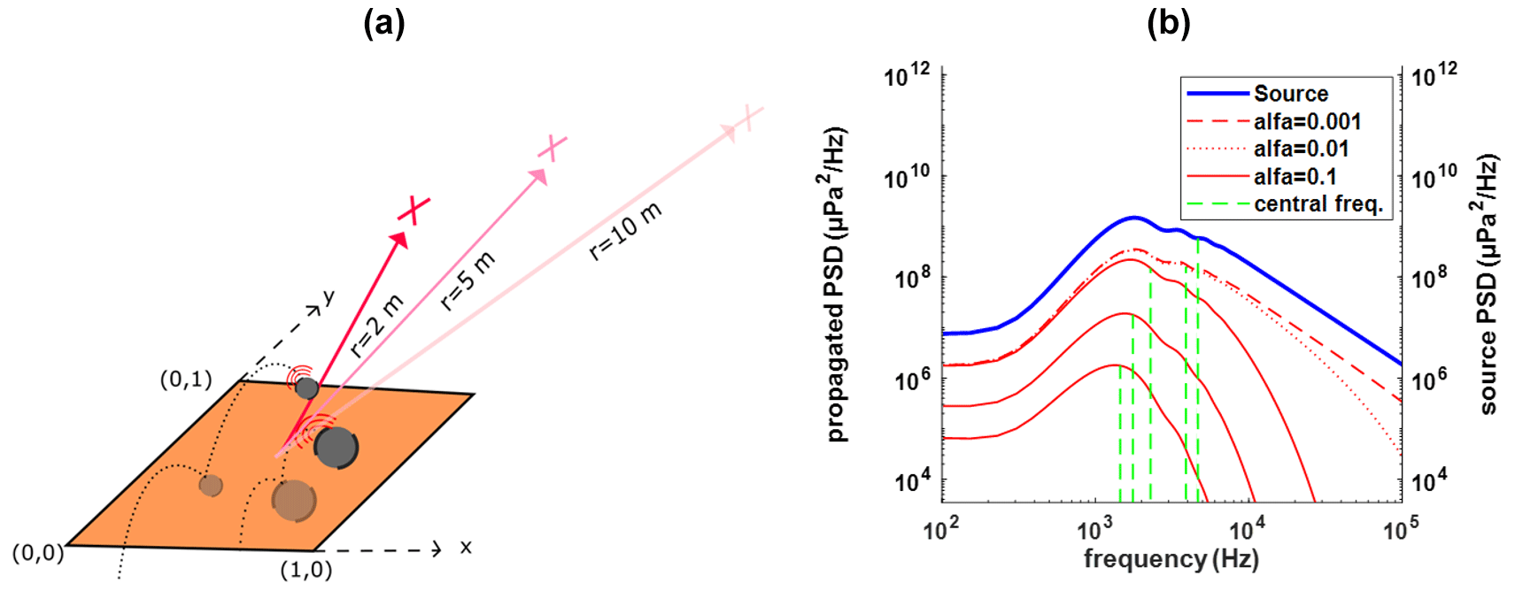
Figure 1 (a) Representation of a unit surface acoustic source with multiple particle–particle impacts. (b) The power spectral density (PSD) of the modeled source signal in blue (r=1 m), with the propagated signals in red at r=2, 5 and 10 m. Different red line styles correspond to different dimensionless attenuation coefficients for the spherical model (${\mathit{\alpha }}_{{\mathit{\lambda }}_{\mathrm{s}}})$. The green vertical lines represent the central frequency of each PSD.

The physical model of Nasr et al. (2022) calculates the acoustic source of bedload SGN as in Eq. (1) starting from the hydraulic conditions of the river and bedload characteristics (flux and GSD). The latest then modeled the distribution of the propagated SGN in the river (p) and compared it to measured values. Nasr et al. (2022) concluded that the comparison of the modeled SGN with the measured values is highly dependent on the chosen empirical formula for impact rate (η) and velocity (U_c) (Eq. 1), which are parameters difficult to validate and measure in the field. In our inversion model, we use the measured SGN (p) and the transmission loss function (TL) to calculate the bedload SGN source (s), which is independent of the propagation characteristics of the river. Equation (1) shows the dependency of the source s on the bedload flux; however, following the results of Nasr et al. (2022) and the limitations on measuring or estimating parameters such as bedload particle impact rate and velocity, the inversion of Eq. (1) to estimate the bedload flux directly from s is not covered in this article.

3 SGN source inversion method

This section presents the general formulation of the inverse mathematical problem.

3.1 Problem formulation

The purpose of the inversion problem is to estimate the PSD and the spatial distribution of bedload SGN sources in rivers. The problem can be illustrated in Fig. 2, where M bedload SGN sources of constant width W_M are assumed to be distributed on the riverbed with total width W. It is assumed that the specific bedload flux (${\stackrel{\mathrm{‾}}{q}}_{s,x})$ is constant for each band in the streamwise direction (along longitudinal line y); in other words, source power is assumed uniform along a given longitudinal line. This simplifies the geometry of sources as planar strips with infinite lengths in the y direction (Fig. 2). The PSD per unit area s_m(f) (µPa² Hz⁻¹ m⁻²) is defined for each source, with m an integer $\mathrm{1}\le m\le M$. The vector S of dimension [M,1] and with the elements s_m (f) represent all the sources' PSDs distributed in the river.

To solve the inversion problem, the first parameter to be considered is the PSD of acoustic measurements of the bedload SGN. Here, we consider a situation matching with drift boat measurement, where a boat supporting the hydrophone successively measures the associated acoustic SGN at N different positions. Measuring the SGN noise using a freely drifted boat with the flow significantly reduces the hydraulic noise generated by hydrophone resistance to the flow (Geay et al., 2020). N acoustic measurements are thus assumed to be distributed on the river cross-section (x direction Fig. 2), from which we compute a PSD for each drift measurement. The parameter p_n (f) corresponds to the PSD measured by a hydrophone drift at the nth position, with n an integer $\mathrm{1}\le n\le N$. The measured SGN profile is thus represented by the vector P, with dimension [N,1] comprising all measured p_n(f).

Given all sources in the river, the measured PSD p_n(f) is the contribution of all M acoustic sources propagated to the nth measuring position. The contribution of all propagated source signals to the measured PSD can be calculated using the linear equation as follows:

$$\begin{array}{}\text{(7)}& p_n\left(f\right)=\sum _{m=\mathrm{1}}^M{a}_{m,n}\left(f\right)s_m\left(f\right),\end{array}$$

where a_m,n is the attenuation factor that affects the propagated signal of source m when measured by the hydrophone at position n. The attenuation factor a_m,n is calculated for a surface source using the frequency-dependent transmission loss function TL:

$$\begin{array}{}\text{(8)}& a_{m,n}=\underset{x_{m\mathrm{1}},y_{m\mathrm{1}}}{\overset{x_{m\mathrm{2}},y_{m\mathrm{2}}}{\iint }}\mathrm{TL}\left(f\left(k\right),r_{m,n}(x,y,z)\right)\mathrm{d}x\mathrm{d}y,\end{array}$$

where r_m,n is the function that defines the distance between any point within the source m area and a hydrophone at position n with coordinate $\left(x_{\mathrm{hyd},n}{y}_{\mathrm{hyd},n}{z}_{\mathrm{hyd},n}\right)$ such that $r_{m,n}\left(x,y,z\right)$ = $\sqrt{{\left(x-x_{\mathrm{hyd},n}\right)}^{\mathrm{2}}+{\left(y-y_{\mathrm{hyd},n}\right)}^{\mathrm{2}}+{\left(z-z_{\mathrm{hyd},n}\right)}^{\mathrm{2}}}$, and z depends on the geometry of the section (constant for rectangular cross-section). The integral limits x_m1y_m1x_m2 and y_s2 define the boundaries of the source in space. The values of y_m1 and y_m2 were chosen to be much greater than the river width W (length=10 W) to model the infinite length of the source stripe. Finally, when Eq. (7) is applied to the whole domain we obtain the matrix

$$\begin{array}{}\text{(9a)}& \mathbf{P}=\mathbf{A}\cdot \mathit{S}\end{array}$$

$$\begin{array}{}\text{(9b)}& \left(\begin{array}{l}{\mathrm{p}}_{\mathrm{1}}\left(f\right)\\ \mathrm{⋮}\\ {\mathrm{p}}_N\left(f\right)\end{array}\right)=\left(\begin{array}{lll}{\mathrm{a}}_{\mathrm{1},\mathrm{1}}\left(f\right)& \mathrm{\cdots }& {\mathrm{a}}_{M,\mathrm{1}}\left(f\right)\\ \mathrm{⋮}& \mathrm{\ddots }& \mathrm{⋮}\\ {\mathrm{a}}_{\mathrm{1},N}\left(f\right)& \mathrm{\cdots }& {\mathrm{a}}_{M,N}\left(f\right)\end{array}\right)\cdot \left(\begin{array}{l}{s}_{\mathrm{1}}\left(f\right)\\ \mathrm{⋮}\\ s_M\left(f\right)\end{array}\right),\end{array}$$

where A is the attenuation. The multiplication of the nth raw element of attenuation matrix A with the sources vector S corresponds to the propagation of all sources in the river to the nth hydrophone position.

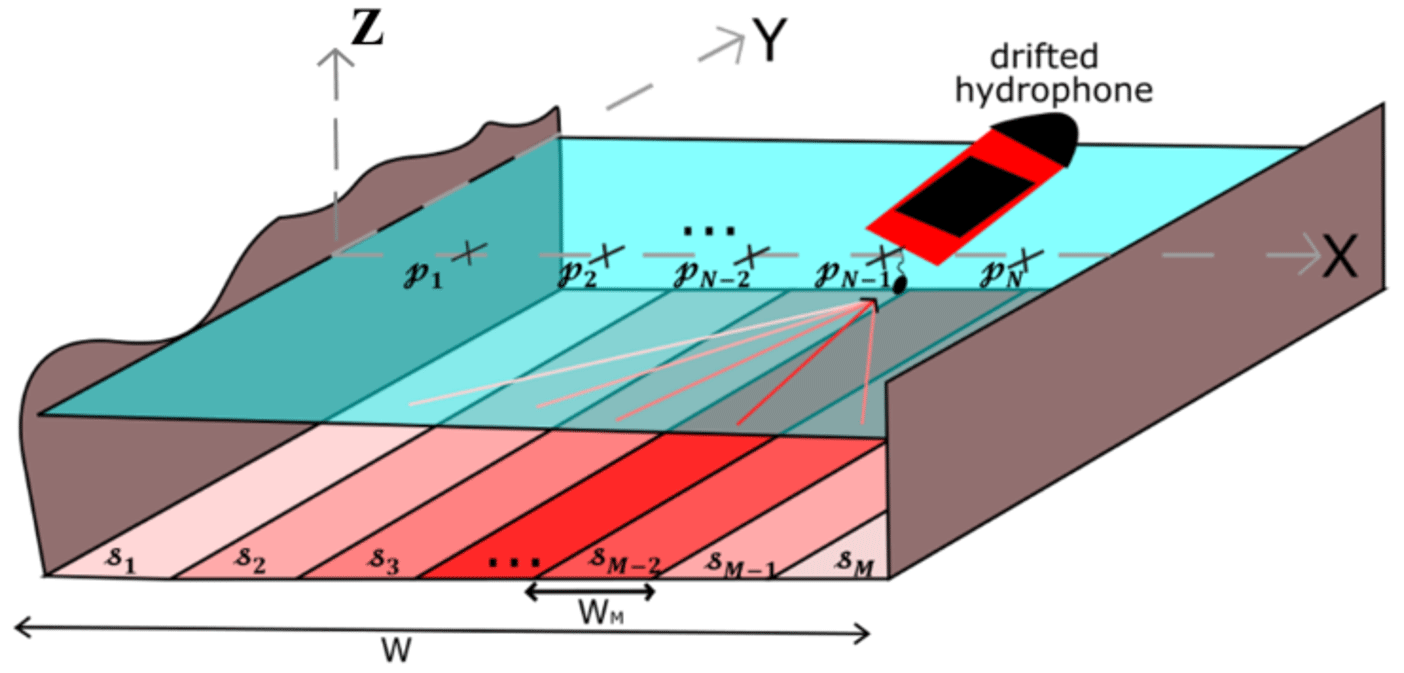
Figure 2 Comprehensive presentation of the inversion problem geometry, where s_m corresponds to different bedload SGN sources on the riverbed. The difference in color corresponds to different SGN source intensities. The points p_n correspond to SGN measurements at different positions by the drifted hydrophone method.

3.2 Solution to the inversion problem

At this stage, we consider that we know the measured acoustic matrix P and assume that the attenuation matrix A is computed (Eqs. 3 and 4) with a known (measured) attenuation term α_λ. We seek the solution $\widehat{\mathit{S}}$ of the vector S, which allows the modeled vector $\widehat{\mathit{P}}=\mathbf{A}\cdot \widehat{\mathit{S}}$ to best fit the measured acoustic P vector. A traditional approach for this type of problem is the least square (LS) method, with an optimization algorithm that works on the minimization of squared residual errors between P and $\widehat{\mathit{P}}$. The error vector ϵ can be written as in Eq. (10a), and the optimization of the problem solving $\widehat{\mathit{S}}$ is presented in Eq. (10b), where the argument of the minimum of ϵ(arg min(ϵ)) is the value of $\widehat{\mathit{S}}$ that minimizes ϵ.

$$\begin{array}{}\text{(10a)}& {\displaystyle }\mathit{ϵ}=\mathit{P}-\widehat{\mathit{P}}=\mathit{P}-\mathbf{A}\cdot \widehat{\mathit{S}},\text{(10b)}& {\displaystyle }\widehat{\mathit{S}}=\arg min\left(\mathit{ϵ}\right)\end{array}$$

The relation between the number of sources M and measurements N determines the type of algebraic system for the problem in Eq. (9). If the number of sources exceeds the number of measurements (M>N), then the equation is considered under-determined. In this case, there are more unknowns than equations, and an infinite number of solutions of $\widehat{\mathit{S}}$ exists. On the other hand, if M<N, there are more independent equations than unknowns, and the equation system is considered over-determined. In the latest case, it is shown by Nelson and Yoon (2000) that the optimal solution for the acoustic source vector, which ensures minimization of Eq. (10b), is

$$\begin{array}{}\text{(11)}& \widehat{\mathit{S}}={\mathbf{A}}^{+}\cdot \mathit{P},\end{array}$$

where ${\mathbf{A}}^{+}={\left({\mathbf{A}}^{\mathrm{t}}\cdot \mathbf{A}\right)}^{-\mathrm{1}}\cdot {\mathbf{A}}^{\mathrm{t}}$ is the pseudo-inverse of the matrix A, and A^t is the transpose matrix.

The pseudo-inverse algorithm for non-square matrixes exhibits a common drawback where the solution $\widehat{\mathit{S}}$ may suffer from divergence (instability) under slight variations in the value of the elements of A or P. The problem's ability to estimate stable or unstable solution $\widehat{\mathit{S}}$ is called conditioning of the problem. The conditioning of the problem is quantified by the condition number σ of the matrix A to be inverse. This condition number is defined as σ(f)$=∥\mathbf{A}∥\cdot ∥{\mathbf{A}}^{-}∥$, where ∥A∥ is the 2-norm of the matrix A (Golub et al., 1996). A system with a high value of σ is considered an ill-conditioned system that generates high instability of the solution $\widehat{\mathit{S}}$, leading to a situation where a small deviation or error in A and P can lead to a large deviation in $\widehat{\mathit{S}}$. In contrast, a value σ closer to 1 is a well-conditioned system. A problem with a condition number σ<10³ can be considered to be well conditioned (Arthur et al., 2017).

When the number of hydrophone measurements (N) is significantly greater than the number of sources (M), or when the measurements are closely spaced, the resulting matrix A may have rows with attenuation factor values (a_m,n) that are very similar to each other. This similarity in values can lead to a matrix that lacks full rank, known as a rank-deficient matrix. A classical solution for such instability problems is the non-negative least square (NNLS) method, a constrained least square problem where the values in the solution vector $\widehat{\mathit{S}}$ are strictly positive values.

In the case of the number of sources equal to the number of measuring points (N=M), the pseudo-inverse matrix is simply the algebraic inverse matrix of A and $\widehat{\mathit{S}}={\mathbf{A}}^{-}\cdot \mathit{P}$.

The MATLAB function lsqnonneg (), which follows the NNLS algorithm, is used for solving the inversion problem.

3.3 Numerical testing of the inversion model

Several numerical tests are presented here to illustrate the behavior and limits of the proposed inversion model. The tested section is composed of a 10 m wide river, with a rectangular section and a water depth of 1 m. Bedload SGN sources are assumed to be distributed on the riverbed in the form of bands, as in Fig. 2. The total bedload active channel width – the sections with bedload transport – equals 4 m. Within the active bedload channel, the source PSD s_m is computed with Nasr et al. (2021); outside s_m is zero. Three different configurations of bedload transport distribution have been tested (single, dual and triple channels); they correspond to the number of separated bedload active channels in the river cross-section (Fig. 3). The considered length of the sources along the river direction is 100 m upstream and 100 m downstream of the section.

We consider the number of simulated acoustic measurements equal to the number of sources (M=N), and the measurements are positioned above each source's center (Fig. 2). The simulated PSD p_n values are calculated using the PSD of the acoustic sources s_m as in Eq. (7). The spherical propagation model is used with an attenuation coefficient ${\mathit{\alpha }}_{{\mathit{\lambda }}_{\mathrm{s}}}=\mathrm{0.05}$ (equivalent to propagation environment for a river with slope S≈1 %).

Figure 3 shows the cross-sectional distribution of the frequency-integrated source power $P_{{\mathrm{s}}_m}$ (µPa² m⁻², blue line) and simulated measured power $P_{{\mathrm{p}}_n}$ (µPa², red line) for different configurations, such that

$$\begin{array}{}\text{(12a)}& {\displaystyle }{P}_{{\mathrm{s}}_m}={\int }_{f_{\min }}^{f_{\max }}{s}_m\left(f\right)\mathrm{d}f\text{(12b)}& {\displaystyle }{P}_{{\mathrm{p}}_n}={\int }_{f_{\min }}^{f_{\max }}{\mathrm{p}}_n\left(f\right)\mathrm{d}f.\end{array}$$

In the absence of hydraulic noise at low frequencies (Geay, 2013), f_min=0 kHz, and f_max=150 kHz, which is the maximum value of the simulated PSD.

In the first place, no extrinsic acoustic noise has been considered. Using the simulated acoustic profile P and Eq. (11), the source PSDs are inverted by the NNLS method for different tests. Figure 3 shows that the inverse source power profiles $P_{\widehat{s_m}}$ (black line) coincide with the generated profile (in blue) for all tests, suggesting good prediction and solution of NNLS under accurate measuring conditions.

To account for possible uncertainty in field measurements, a noise has been added to the simulated p_n. The noise was added in the form of a white noise signal convolved with the SGN signal. The resulting acoustic profiles are plotted (dashed red lines) in Fig. 3. In the presence of noise, the inverse source power $P_{\widehat{s_m}}$ (dashed black lines) is distinct from the generated source power profile (in blue). The results' errors are limited not only to the intensity of sources but also the appearance of sources outside the bedload active channel. Nonetheless, the average cross-sectional power of the inverse source profile (integration of the curve divided by the width) is between 2.35–2.43 µPa² m⁻¹, which is close to the corresponding value for that for the imposed source (2.36 µPa² m⁻¹). This means that if we consider the total inverse power, the error is more limited to the localization of these sources.

To numerically assess the results, a variance-explained accuracy measure (VEcv) parameter is introduced (Li, 2017). The advantage of this dimensionless accuracy measure VEcv is that it is independent from data mean, and variance according to its definition. A VEcv close to one means good accuracy of the model. The VEcv is calculated as follows:

$$\begin{array}{}\text{(13)}& \mathrm{VEcv}=\left(\mathrm{1}-{\displaystyle \frac{\sum _{m=\mathrm{1}}^M{\left(P_{{\mathrm{s}}_m}-P_{\widehat{s_m}}\right)}^{\mathrm{2}}}{\sum _{m=\mathrm{1}}^M{\left(P_{{\mathrm{s}}_m}-{\stackrel{\mathrm{‾}}{P}}_{\mathrm{s}}\right)}^{\mathrm{2}}}}\right),\end{array}$$

where $P_{\widehat{s_m}}$ is the inverse source power, and $P_{{\mathrm{s}}_m}$ is the imposed source power, ${\stackrel{\mathrm{‾}}{P}}_{\mathrm{s}}$ is the average of total imposed source power. The values of VEcv have been calculated for each simulation and are presented in the titles of Fig. 3. The VEcv values show that the inversion model can have good performance even in the presence of noise (VEcv ≈ 0.9 close to 1). However, the VEcv values relatively decrease when the number of bedload active channels increases, suggesting a higher sensitivity of the model to field uncertainty under complex bedload distribution.

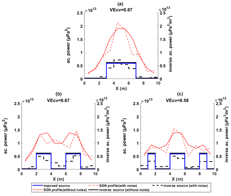
Figure 3 Numerical test results of the inversion model for (a) single-, (b) double- and (c) triple-bedload-active-width-channel configurations. The figures compare the simulated SGN source acoustic power ${\mathit{P}}_{{\mathrm{s}}_m}$ (in blue; µPa² m⁻²) with the inverse source power ${\mathit{P}}_{{\widehat{s}}_m}$ (in black) without noise (continuous line) and with noise (dashed line). The figure also compares the measured SGN acoustic power ${\mathit{P}}_{{\mathrm{p}}_n}$ (in red; µPa²) without noise (continuous line) and with noise (dashed line).

4 Inversion model validation

In this section, we present two experiments for testing and validating the inversion model.

4.1 Validation with active test measurements

This first experiment aims to test the inversion model under controlled source conditions. It is technically challenging to deploy a sound source with a scale comparable to the SGN source in the river. Instead, in this experiment, we use a loudspeaker in the river as a source with a known signal and location. The test consists of measuring the emitted sound by the loudspeaker at different locations in the river and then testing the ability of the inversion model to retrieve the active source's location and PSD.

4.1.1 Isère river and experimental setup

This experiment was carried out in the Isère river in southeastern France. The measuring site is located next to Grenoble (45^∘11^′55.0” N, 5^∘46^′11.4" E) on a pedestrian's footbridge crossing the river. The local average slope for the measured section is 0.05 %, with a width of 60 m, and the annual average flow is 180 m³ s⁻¹. The riverbed is composed of gravel, with average $D_{\mathrm{50},\mathrm{bed}}=\mathrm{23}$ mm measured with the Wolman (1954) sampling protocol for the exposed riverbed. During the time of measurement, on 25 August 2022, the average flow was 110 m³ s⁻¹. Under this flow condition, the Isère is characterized by low hydraulic noises generated by the flow turbulence at low frequencies (Geay, 2013), as well as no bedload SGN.

We used a waterproof piezoelectric Lubell loudspeaker with a 23 cm diameter (model LL916H; http://www.lubell.com/LL916.html, last access: 9 November 2023), characterized by a quasi-flat (±10 dB) frequency response between 500–21 000 Hz. The loudspeaker is connected to an emission RTSYS system (TR-SDA14), which controls the emitted signal by a .wav file stored inside the RTSYS. The chosen transmission signal is a logarithmic frequency modulation between 500 and 21 000 Hz in 0.25 s. The .wav file for the sound emitted by the loudspeaker is provided in the Supplement. The loudspeaker signal was characterized in a lake next to Grenoble in France. The water depth at the testing position was around 5.5 m. The source was positioned 3 m under the water's surface. The emitted signals were measured at a 1 m horizontal distance from the source with an HTI-99 hydrophone (High Tech, Inc., http://www.hightechincusa.com, last access: 9 November 2023) with a sensitivity of −199.8 dB and characterized by a flat frequency response (∓ 3 dB) between 2 Hz and 125 kHz. The hydrophone was connected to the EA-SDA14 card acquisition system (RTSYS company) recording the acoustic signal in .wav format with a sampling frequency of 312 kHz. Different orientations of the loudspeaker in space have been tested. A PSD (µPa² Hz⁻¹) was calculated for each measured chirp. Finally, using Eq. (6b), the surface PSD of the loudspeaker (µPa² Hz⁻¹ m⁻²) was calculated by dividing the measured PSD by the TL function term. The TL function was calculated considering the dimension of the source for r=1 m and ${\mathit{\alpha }}_{{\mathit{\lambda }}_{\mathrm{s}}}=\mathrm{0}$, attenuation being only due to geometrical spreading in a lake. The result of the source power is presented in Fig. 4c (green lines) with the 5 %, 50 % and 95 % percentiles.

In the Isère, the loudspeaker was deployed from the bridge to the riverbed at the position x_source=48 and y_source=3 m (in the downstream direction). At this position, the average water column depth is 1.5 m. The signals were emitted from the source in an endless loop. We measured the acoustic profiles every 2 m between x=8 and x=56, with the same hydrophone and acquisition system presented above. The protocol was identical to that of Geay et al. (2020), with the hydrophone mounted on a floating river board (40 cm below the water surface) and freely drifting from the bridge (drift position between y=2 m and y=4 m from the bridge). The acoustic measurements were carried out in N different positions on the river cross-section. For each drift n located at x_n, we measured the power spectrum of all signals' impulsion during the drift and determined the median spectrum PSD_n. Each drift n is now characterized by its coordinate (x_ny_n=3 m) and a median spectrum PSD_n.

Inversion of the active acoustic source requires the definition of parameters presented in Eq. (9) (P and S vectors and A matrix). For the measured acoustic profile, the vector P is composed of the 25 measured median power spectra defined above, p_n(f)=PSD_n(f) ($\mathrm{1}<n<\mathrm{25}$). We considered that $N=M=\mathrm{25}$ and incorporate 25 square sources with 2 m sides distributed between $\mathrm{7}\le x\le \mathrm{56},$ with unknown source power spectra s_m(f). The transmission loss parameters a_m,n(f) have been calculated using Eq. (8) for the spherical model. The attenuation coefficients presented in Eq. (4), ${\mathit{\alpha }}_{{\mathit{\lambda }}_s}={\mathrm{10}}^{-\mathrm{4}}$, have been estimated following the protocol proposed by Geay et al. (2019) during the measurement day. To reduce the computational load, the sources' spectra s_m(f) have been calculated using the third-octave band of the measured spectrum.

The area of the inverse sources in this application is 4 m² (2 m side squares), which is different than that of the loudspeaker area ≈0.04 m². In this case, an area correction factor was applied to the inverse results in order to compare it with the loudspeaker source signal measured in the lake. The area correction factor was calculated as the ratio between the TL function calculated as in Eq. (6b) for the inverse source area and for the loudspeaker area.

4.1.2 Results

Figure 4b plots the measured acoustic power profile $P_{{\mathrm{p}}_n}$ (red line), calculated with Eq. (12) between frequencies of 500–21 000 Hz. The measured spectra show different intensities depending on the distance from the active source. No significant variation in the spectral distribution is observed with propagation due to the relatively low attenuation coefficient in the Isère.

The results of the inverse power profile $\left(P_{\widehat{s_m}}\right)$ are plotted in Fig. 4b (black line). The results show that the inversion model successfully captures the active source location between x=47 and x=49 (m=21). However, some residual sources have been modeled mainly around the active source location and at other locations in the river. As in the numerical test with noise (Sect. 3.3), it is suspectable that measurement uncertainty contributes to such residual sources as they coincide with the perturbation in the measured acoustic profile (e.g., x=26 and 35 m).

The spectra of each drift (p_n(f)) are presented in Fig. 4c (continuous faded lines), and the color index corresponds to the distance of the spectrum from the deployed loudspeaker. Figure 4c shows the inverse source spectrum in the proximity of the loudspeaker location ${\widehat{s}}_{n=\mathrm{21}}$ (between x=47 and x=49). The results show that the inverse spectra are comparable with the reference spectrum of the source characterized in the lake, which fits within the 5 %–95 % percentiles at most frequencies.

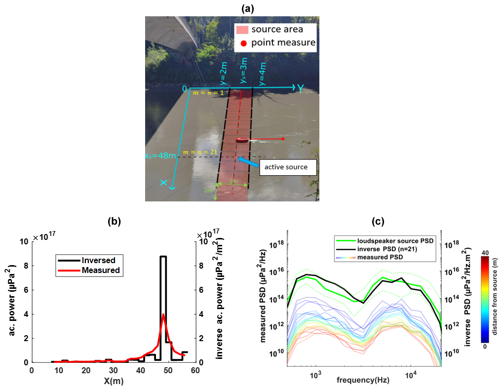
Figure 4 (a) Representation of the geometry of sources and acoustic measurements on the Isère. (b) Measured acoustic power $P_{p_n}$ (µPa²; red line) and the inverse source power $P_{\widehat{s_m}}$ (µPa² m⁻²; black line). (c) Measured spectrum at each position in the river P_n (µPa² Hz⁻¹; faded color lines). The color index shows the distance of the measurement from the source, which increases from blue to red. The inverse spectrum $\widehat{s_m}$ (µPa² Hz⁻¹ m⁻²; black line) corresponds to the spectrum at 47–49 m (n=21). The green spectrum corresponds to the median of the measured lake spectrum, with the dotted line corresponding to 5 % and 95 % percentiles.

4.2 Validation with passive SGN measurements

4.2.1 Giffre river and experimental setup

In this part, we apply the inversion model to bedload SGN measurements. An experiment was carried out in the Giffre river located in the French Alps. The measured section is under a pedestrian crossing bridge (46^∘${\mathrm{04}}^{\prime }{\mathrm{48.8}}^{\prime \prime }$ N, 6^∘${\mathrm{42}}^{\prime }{\mathrm{19.4}}^{\prime \prime }$ E). The average slope of the section is 0.3 %, and the width is 29 m. Two measurements of SGN and bedload flux were carried out during the melting season on 13 June 2018 and 6 July 2021. On these dates, the flow discharges were 50 and 26 m³ s⁻¹, respectively, with 0.9 and 0.7 m average water depth (d).

Acoustic measurements were obtained using HTI-99 hydrophones (with sensitivity: −200.1 dB in 2018 and −199.8 dB in 2021) and the RTSYS acquisition system with the drift protocol (Geay et al., 2020). The drifts were 20 to 30 m long (in the y direction) with the hydrophone set up 30 cm below the surface. Several repetitions of drifts have been performed at each cross-sectional position x_n to account for measurement uncertainty and temporal variability. For each drift at the location x_n, we computed the median measured PSD_n(f). In the presence of repetition of drifts at the same location x_n, we averaged the PSD_n.

Bedload particles were sampled from the bridge using a handheld Elwha sampler with dimensions of 203×152 mm. Sampling was performed at various cross-section positions following the procedures proposed by (Edwards and Glysson, 1999) with variable repetitions. Each sample was dried, sieved and weighed to calculate the transport rate and grain size distribution (GSD). We calculated a specific bedload flux q_s,i (g s⁻¹ m⁻¹) as follows:

$$\begin{array}{}\text{(14)}& q_{\mathrm{s},i}={\displaystyle \frac{m_i}{t_i\times W_{\mathrm{sampler}}}},\end{array}$$

where W_sampler is the inlet width of the sampler, and m_i and t_i are the mass and the duration of sampling, respectively. The average bedload flux profile has been calculated within N windows, each 2 m in width. Each window is centered on an acoustic point measurement x_n as for the acoustic source. The average bedload flux ${\stackrel{\mathrm{‾}}{q}}_{\mathrm{s},n}$ (g s⁻¹ m⁻¹) for the window n is calculated by averaging the values of q_s,i contained inside the spatial window n.

The geometry of the SGN sources used is similar to Fig. 2 with a length extended for each source between $y=-\mathrm{150}$ m and y=150 m, which account for the infinite-length assumption of the SGN sources.

Two active tests following the protocol of Geay et al. (2019) have been carried out to characterize the propagation environment in the Giffre during the two measurement days in 2018 and 2021. The attenuation coefficients estimated for the spherical model are ${\mathit{\alpha }}_{{\mathit{\lambda }}_{\mathrm{s}}}=\mathrm{0.006}$ and ${\mathit{\alpha }}_{{\mathit{\lambda }}_{\mathrm{s}}}=\mathrm{0.004}$ for 2018 and 2021, respectively. The attenuation coefficients were measured up to a maximum frequency of 20 kHz and extrapolated at higher frequencies assuming a linear regression.

4.2.2 Results

Figure 5 presents the averaged profile for bedload flux and the measured acoustic power for both experiments. The left and right riverbanks are located at x=0 and x=29, respectively. In both measurements, the bedload flux profile is composed of a main transported channel localized at the right section of the river (peak at x=20). The average specific bedload flux calculated for both experiments shows that the bedload transport intensity in 2018 was 15 times more than that of 2021 (328 g s⁻¹ m⁻¹ compared to 22 g s⁻¹ m⁻¹). The measured SGN profiles show a coherent variation in acoustic power with the bedload flux in the river cross-section. However, the decrease in the acoustic power in the left part of the river section (between x=0 and x=13) does not correspond to the same intensity decrease in bedload flux.

Acoustic recording samples from both experiments are presented in the Supplement. After analyzing and listening to the recordings at different frequencies, bedload SGN can be clearly heard above 800 Hz. At frequencies lower than 400 Hz, the main source of noise is the hydraulic noise induced by the flow turbulence in the river and around the hydrophone. The mean measured PSDs are presented in Fig. 6a and b. The central frequencies calculated for the mean PSD are 5.6 and 10 kHz for 2018 and 2021, respectively. The difference in central frequency is mainly induced by the different grain size distributions sampled during both experiments (the average D₅₀ sampled in 2018 was 6.8, and it was 3 mm in 2021). In addition, the attenuation of the SGN signal is more important during 2018 measurements due to more water turbulence induced by the higher flow. The higher attenuation contributes to the decrease in the measured central frequency, as explained in Sect. 2.3.

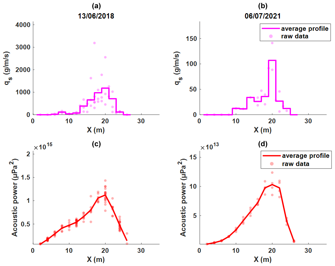
Figure 5 Measured bedload flux (a) in the 2018 experiment and (b) in the 2021 experiment. The measured acoustic power (c) in the 2018 experiment (d) in the 2021 experiment.

Figure 6a and b also present the mean inverse PSD. The central frequency calculated for the inverse PSD shows an increase in both experiments compared to the measured value (an increase from 5.6 to 11 kHz in 2018 and 10 to 19.1 kHz in 2021). A visual comparison shows that other than the power value, the main difference is the slope of the PSD at higher frequencies. In contrast, the PSD shape at lower frequencies has not been significantly affected. This shows that the inversion model corrects the attenuated signal at high frequencies, as explained in Sect. 2.3 and Fig. 1.

Figure 6c and d present the inverse power profile $P_{\widehat{s_m}}(\mathrm{\mu }{\mathrm{Pa}}^{\mathrm{2}}$ m⁻²), which can be compared to the measured profile $P_{{\mathrm{p}}_n}$. The inverse power per unit area is 1 order of magnitude less than the measured power since each source contributes (by sound propagation and in a cumulative way) to each measured value. Moreover, the source spectrum was calculated for a distance of 1 m from the source, while the measurements with the drift hydrophone were taken at a smaller distance (∼30 cm below the water surface <1 m).

To compare the measured and inverse power with the bedload flux profile, we scaled the signals by computing the ratio between the local value and the total cross-sectional value for each profile. Results are plotted in Figs. 6e and 6f, which show a better synchronization of the bedload flux profile with the inverse power profile than the measured profile. This is particularly evident when considering the peaks and the sharp transition to low transport at the side of the section.

To numerically compare the profiles, the VEcv value is calculated for both the relative source and the relative measured profile in reference to the relative bedload flux profile. The values of VEcv are presented in Figs. 6e and 6f, confirming that the inverse source profile better illustrates the bedload flux than the measured SGN profile in both experiments. However, the improvement of VEcv in the 2021 experiment is less than that for the 2018 experiment.

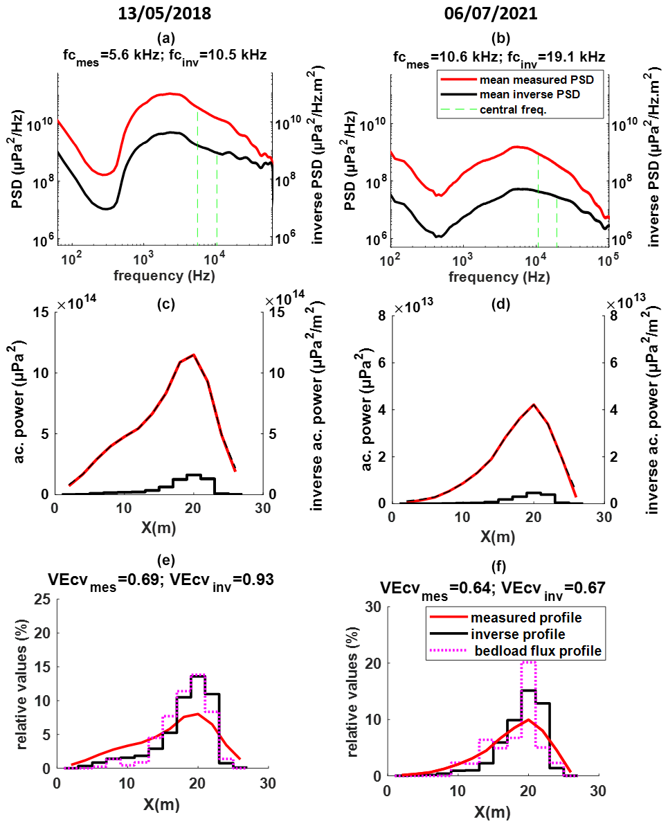
Figure 6 Mean measured PSD p_n (in red) and inverse PSD $\widehat{s_m}$ (in black) for 2018 and 2021 in (a) 2018 and (b) 2021. Mean measured power ${\mathit{P}}_{{\mathrm{p}}_n}$ (in red) and inverse power ${\mathit{P}}_{\widehat{s_m}}$ (in black) for the (c) 2018 and (d) 2021 experiments. Relative profiles for (e) 2018 and (f) 2021; the relative bedload flux profile ${\stackrel{\mathrm{‾}}{q}}_{\mathrm{s},n}$ is in magenta.

To study the effect of inversion on the acoustic power–bedload flux relation, the measured bedload flux value at measuring position n is plotted against the corresponding value of measured acoustic power and inverse acoustic power for both the 2018 and 2021 experiments (Fig. 7). Depending on the experiment, we can differentiate two different trends for the measured acoustic power.

Power laws have been fitted in Fig. 7 to the measured data by applying reduced major axis (RMA) regression, which is used when data on both axes have uncertainties (Smith, 2009). The fitted power laws presented in Fig. 7 show two very distinct trends, with more than 1 order of magnitude of bedload flux for the same acoustic power values. On the other hand, the relationships obtained with the inverse data show a better continuation with less dispersion between the two experiments, allowing a unique fit with a relatively good Pearson correlation coefficient (R²=0.79).

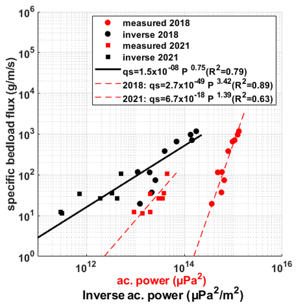
Figure 7 Local values of bedload flux vs. local values of measured acoustic power (in red) and inverse acoustic power (in black).

5 Discussion

5.1 Dealing with uncertainties

The numerical testing in Sect. 3.3 (Fig. 3) showed that the comparison between the simulated and the inverse source profile is impacted by the presence of acoustic noise in the signal. In addition, the Isère experiment's results (Fig. 4b) have shown that extraneous noise sources appeared in different positions with different intensities due to uncertainty and perturbations in the measured acoustic profile. Meanwhile, the data collected on the Giffre river show variabilities in acoustic measurements as well as the bedload flux measurements (Fig. 5). Thus, the inversion results of the Giffre application should consider the potential errors due to measuring uncertainties. These uncertainties have been calculated following Geay et al. (2020), who estimated the relative uncertainty in acoustic measurements at 8 % and 6 % and the relative uncertainties associated with bedload flux at 29 % and 32 % for 2018 and 2021, respectively. Several factors can contribute to the variability in bedload flux measurements, such as the efficiency of bedload samplers itself under different hydraulic conditions (Childers, 1999; Bunte et al., 2008). Moreover, the uncertainty in bedload sampling is also affected by the position of the sampler on the river bed (Vericat et al., 2006), where difficulties in controlling the exact position of the Elwha sampler were reported during our field measurements. Furthermore, in the 2021 experiment, the number of bedload sampling repetitions was limited due to unstable flow conditions generated by a rainfall event after the beginning of the experiment. Then, the main difficulty in comparing inverse acoustic measurements with the bedload flux profile is mainly related to the quality of bedload flux sampling. Additional uncertainties also concern the attenuation coefficients obtained by fitting measurements of active test data showing variability of up to a factor of 5 around the best fit.

5.2 Improvement of the calibration curve

The hydrophone measures not only its close environment but all sounds propagating in the river section. The cross-section integration results depend on the local conditions, which can change with discharge, as shown in Figs. 6c and 6d. This explains the two different fits between bedload flux and acoustic power obtained for the Giffre river in Fig. 7. In addition, the high-power coefficients (1.4–3.4), greater than unity as predicted by the theory (Nasr et al., 2022), are also a consequence of the overestimation of the actual source energy. The global calibration curve of bedload flux obtained by Nasr et al. (2022) is based on the average cross-sectional acoustic power values. The effects discussed here have probably contributed to part of the variability obtained when they fit bedload flux as a function of acoustic power. More importantly, the global calibration curve may also generate an overestimation of bedload flux under certain conditions. For example, this calibration curve has been tested on the Drac river (a tributary of the Isère), which is characterized by good sound propagation of SGN and a well-localized bedload channel. The result was an overestimation of the annual average bedload flux by a factor of more than 3.

Figure 7 shows that reducing these effects by inverting the acoustic power gives access to a better adjustment of the data obtained under different bedload transport conditions between the 2018 and 2021 experiments. This offers good potential for improving the global calibration curve (Geay et al., 2020; Nasr et al., 2023) by adjusting a new function after inverting their whole data set. We used the inversion model on the data set of the global calibration curve presented by Nasr et al. (2023), which consists of 42 experiments of simultaneous bedload flux and acoustic measurements collected in 14 different rivers, covering a wide range of properties (e.g., slope, bedload intensity and granulometry). The inversion model has been applied to all rivers, similarly to the Giffre river application. In the case of the absence of an active test on some rivers, a slope-based empirical formula derived from field data (Geay et al., 2019; Nasr, 2023) has been used to estimate the attenuation coefficient:

$$\begin{array}{}\text{(15)}& {\mathit{\alpha }}_{\mathrm{s}}=\mathrm{1720}{I}^{\mathrm{2.28}},\end{array}$$

where α_s is the dimensionless attenuation coefficient for the spherical model presented in Eq. (5), and I is the local riverbed slope measured 100 m upstream and downstream of the section where the active test was conducted. The relation above is obtained from a data set on 14 different rivers with slope varying between 0.02–2.5 %. The correlation coefficient (R²) of this relation is 0.87, which shows that the local riverbed slope is a good proxy for characterizing the propagation environment in the river. The data supporting Eq. (15) are presented in the Supplement (Table S2).

Figure 8 shows the global calibration curve using the cross-sectional average measured acoustic power and the inverse calibration curve using the corresponding cross-sectional average inverse acoustic power. Comparing both calibration curves shows that, when using inverse acoustic power, there is a minor decrease in variability (an increase in R² from 0.72 to 0.74) and a change in the fitted function with a lower power coefficient (decrease from 0.72 to 0.67). However, the main differences between these two calibration curves on bedload flux estimation cannot be concluded from the change in the correlation coefficient R². It should be noted that using the different global calibration curves will lead to different bedload flux estimation for the same experiment (Fig. 8). The main difference between these two calibrations will require investigations with field measurements.

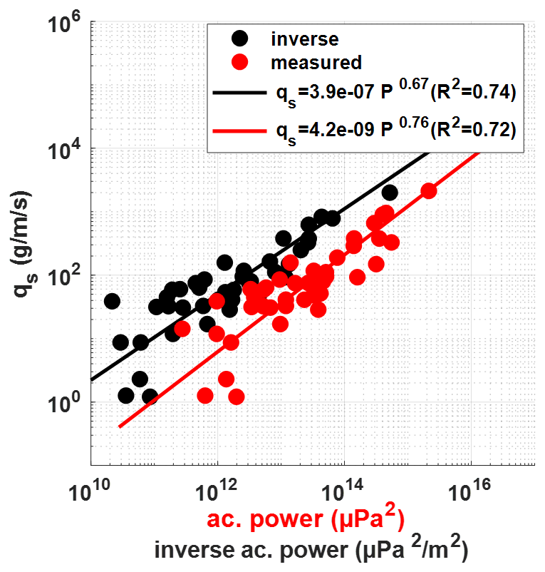
Figure 8 Comparison of global calibration curve fitted with cross-sectional average acoustic power (in red; Nasr et al., 2023) and the readjusted curve fitted with cross-sectional average inverse acoustic power (in black).

5.3 Grain size detection

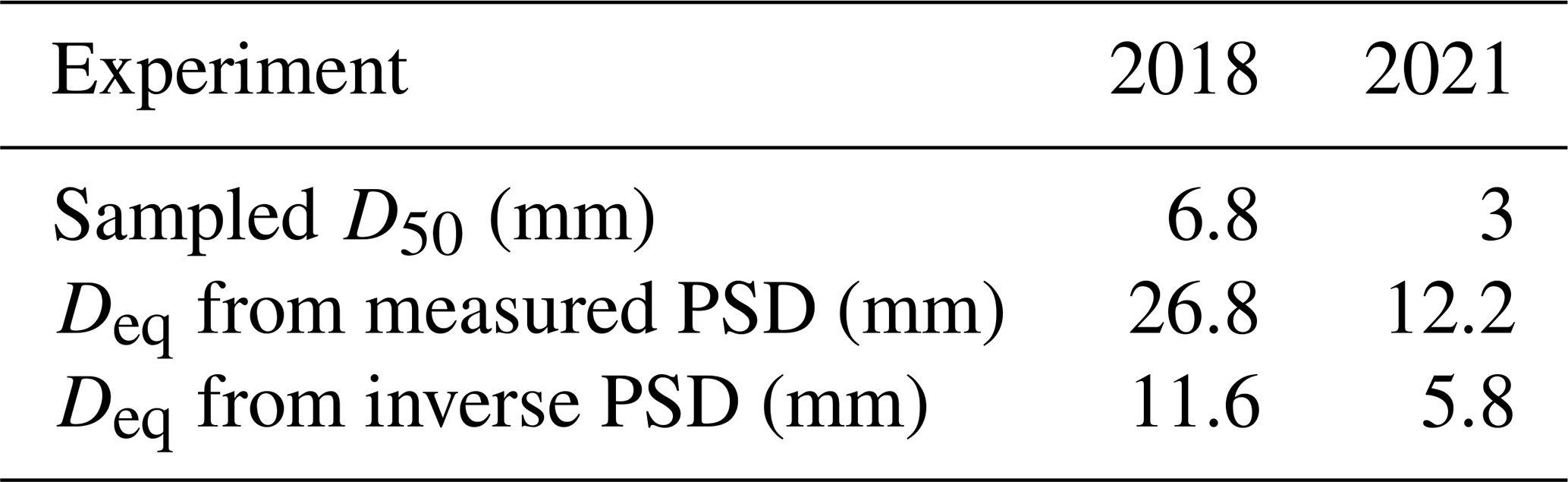
In lab experiments, the frequency content of the SGN has been well correlated with particle diameter (Thorne, 1985, 1986). However, in rivers, the attenuation of the SGN signal at high frequency is responsible for the underestimation of bedload GSD using acoustic measurements (Geay et al., 2018). The results in Fig. 8 show a noticeable correction of the inverse PSD at high frequencies. To quantify the effect of inversion on bedload GSD estimation, the equivalent diameter D_eq is computed by the regress empirical formula of Thorne (1985) as a function of central frequency:

$$\begin{array}{}\text{(16)}& D_{\mathrm{eq}}={\displaystyle \frac{\mathrm{430}}{f^{\mathrm{1.136}}}}.\end{array}$$

Table 1 shows the computed D_eq compared to the measured D₅₀ values, which show that the estimated diameters using SGN measurements overestimated the measured bedload diameter. This overestimation is reduced when using the inverse source PSD. No definitive conclusion can be made on the effect of the inversion model on GSD estimation using Eq. (16) as this experimental law has been carried out in controlled conditions using uniform grain size mixtures. However, the results in Table 1 suggest a real improvement with the inverse signal. Additional effort can be made into GSD estimation by testing the model proposed by Petrut et al. (2018) for a bedload mixture using the inverse signal; however, it is beyond the scope of this article.

Table 1 Comparison of measured bedload D₅₀ with estimated bedload equivalent diameter using measured and inverse PSD.

6 Conclusions

In this article, we present a new approach for the treatment of hydrophone measurements for bedload flux monitoring in rivers. This approach considers an inversion model for the measured acoustic profile of bedload self-generated noise (SGN). The model seeks to locate the sources of SGN and calculates their power spectral density using a system of linear algebraic equations which combines acoustic measurements with acoustic signal transmission loss functions describing the propagation environment of the river.

Numerical testing shows good performance of the model with variable degrees depending on the number of separated bedload active channels in the river cross-section and uncertainty in the measured acoustic profile. Field testing of the model on the Giffre river during two very different hydraulic conditions shows that the inversion model successively corrected the attenuation of the signal PSD. The signal correction by inversion compensates for loss of acoustic power due to the propagation mainly at high frequencies. Direct bedload measurements better correlate with inverse acoustic power profiles than measured acoustic power.

The methodology presented in this paper offers new perspectives for continuous bedload monitoring with hydrophones fixed on the riverbank. Because they measure SGN for both near field and far field, they are directly impacted by propagation effects, and consequently calibration is required. This calibration is possible with a reliable qs(P) function associated with the drift measurement and acoustic inversion protocol.

Appendix A: Notations

α	Frequency-dependent attenuation coefficient	m−1
am,n	Attenuation factor	–
αλ	Dimensionless attenuation coefficient	–
αλc	Dimensionless attenuation coefficient for the cylindrical model	–
αλs	Dimensionless attenuation coefficient for the spherical model	–
A	Attenuation matrix	–
A+	Pseudo-inverse of the matrix A	–
${\mathbf{A}}^{--}$	Inverse of the matrix A	–
At	Transpose of the matrix A	–
cf	Celerity of sound in water	m s−1
D	Particle diameter	m
d	Water depth	m
Deq	Bedload equivalent diameter	m
D50	Bedload median diameter	m
e	Energy spectrum density	µPa2 s Hz−1
ϵ	Model error vector	–
f	Frequency	Hz
fc	Central frequency	Hz
fmax	Maximum integration frequency	Hz
fmin	Minimum integration frequency	Hz
I	Riverbed local slope	Hz
i	Bedload sample index	–
k	Diameter class index	–
qs	Specific bedload flux	g s−1 m−1
${\stackrel{\mathrm{‾}}{q}}_{\mathrm{s}}$	Average specific bedload flux	g s−1 m−1
M	Number of sources	–
m	Measurement index	–
N	Number of measurements	–
n	Measurement index	–
Pp	Integrated measured power	Pa2
Ps	Integrated source power	Pa2 m−2
$P_{\widehat{s_m}}$	Integrated inverse power	Pa2 m−2
$\stackrel{\mathrm{‾}}{P_{\mathrm{s}}}$	Average of all source power in the river	Pa2 m−2
p	Measured PSD	µPa2 Hz−1
P	Measured PSD vector	Pa2 Hz−1
$\widehat{\mathit{P}}$	Modeled PSD vector	Pa2 Hz−1
r	Source–hydrophone distance	m
s	PSD for a point source	Pa2 Hz−1
s	Source PSD per unit area	Pa2 Hz−1 m−2
$\widehat{s}$	Inverse PSD per unit area	Pa2 Hz−1 m−2
S	Source PSD vector	Pa2 Hz−1 m−2
$\widehat{\mathit{S}}$	Inverse PSD vector	Pa2 Hz−1 m−2
σ	Condition number	–
TL	Transmission loss function	–
TL1	Geometrical spreading function	–
TL2	Scattering and absorption function	–
VEcv	Variance-explained accuracy measure	–
W	Width of the river	m
WM	Width of the sources	m
xhyd	Hydrophone x coordinate	m
yhyd	Hydrophone y coordinate	m
zhyd	Hydrophone x coordinate	m