the Creative Commons Attribution 4.0 License.
the Creative Commons Attribution 4.0 License.
 | 09 Feb 2024
Path length and sediment transport estimation from DEMs of difference: a signal processing approach
Lindsay Marie Capito
Enrico Pandrin
Walter Bertoldi
Nicola Surian
Simone Bizzi
The difficulties of measuring bedload transport in gravel-bed rivers have given rise to the morphological method wherein sediment transport can be inferred from changes in riverbed elevation and estimates of the distance traveled by sediment: its path length. Because current methods for estimating path length are time- and labor-intensive, we present a method to estimate a characteristic path length from repeat digital elevation models (DEMs of difference, i.e., DoDs). We propose an automated method to extract the spacing between erosional and depositional sites on the DoD by the application of variational mode decomposition (VMD), a signal processing method, to quantify the spacing as a proxy for path length. We developed this method using flume experiments where bed topography and sediment flux were measured and then applied it to published field data with physical path length measured from tracer measurements. Our sediment transport estimates were not significantly different than the measured sediment flux at lower discharges in the lab. However, we observed an underestimation of sediment flux at the higher discharges in the flume study. We interpret this as a limit of the method in confined settings, where sediment transport becomes decoupled from morphological changes. We also explore how the time between survey acquisitions, the morphological active width relative to the channel width, and DoD thresholding techniques affect the proposed method and the potential issues they pose for the morphological method in general.
- Article
(7053 KB) - Full-text XML
- BibTeX
- EndNote


In gravel-bed rivers sediment transport fundamentally controls morphological processes but is notoriously difficult to measure due to its spatial and temporal heterogeneity (Hoey, 1992; McLean and Church, 1999) and measurement uncertainty (Vericat et al., 2006), as well as the logistical challenges of field measurements. The morphological approach is a method to estimate bedload transport based on observed changes in morphology. There have been many implementations of the morphological method since its inception and it has been reviewed extensively (Ashmore and Church, 1998; Brewer and Passmore, 2002; Church, 2006; Vericat et al., 2017). With the increased availability of hydrologic data and modeling capabilities the morphological method has also been applied in two dimensions (x,y) by coupling a 2D hydraulic model to account for sediment routing (Lane et al., 1995; Antoniazza et al., 2019; Bakker et al., 2019). These 2D applications shed light on the functional links between topographic changes and spatial distribution of bedload transport. Antoniazza et al. (2019) quantified the potential errors in estimating sediment transport using a 1D approach where 2D cross-stream sediment fluxes are neglected. The error associated with neglecting the 2D fluxes may be especially important in multi-threaded channels. They also explored how digital elevation model (DEM) accuracy and the frequency of acquisitions affect the estimates of sediment fluxes derived by the morphological method. These 2D applications enhance the accuracy of the morphological method to estimate sediment transport; however, these studies benefited from intensive field campaigns and an accurate accounting of upstream water and sediment supplies, which are often not available in real case studies. In this paper, the desire is to explore novel approaches to apply the morphological method using topographic data alone, as hydraulic and sediment supply data are not available in many applications and management situations.
The morphological method can be formalized based on the sediment continuity equation:
where and are the volumetric sediment flux in and out of the reach, respectively, Δt is the time between surveys, p is the sediment porosity, and ΔV is the change in volume (Ashmore and Church, 1998; Church, 2006). The sediment continuity equation can be solved in several ways, but in addition to ΔV measured from the DoDs, it requires that either the incoming flux or the outgoing flux be defined. In most cases, neither of these fluxes are known, as they are the exact parameters that need to be estimated when applying the morphological method. This conundrum has been addressed by setting a zero-flux boundary, such as a dam or gravel–sand transition (McLean and Church, 1999), by segmenting the reach such that a zero-flux boundary is set between a section of net deposition to one of net erosion (Vericat et al., 2017; Calle et al., 2020), or by measuring flux either into or out of the reach (Grams et al., 2013; Antoniazza et al., 2019).
Alternatively, Eq. (1) can be modified so that active layer depth ds and width ws, as well as the virtual velocity vb, are used:
where ws is the active layer thickness, generally measured by chains and estimated by depth of scour (Church and Haschenburger, 2017), and vb is equal to , L being the distance the particles travel and T the time over which the particles are traveling (Church, 2006). The virtual velocity approach has been successfully applied using tracer gravel to estimate the path length parameter L in a variety of morphological settings (Liébault et al., 2012; Mao et al., 2017; Brenna et al., 2019, 2020; Brenna and Surian, 2023). Unfortunately, tracer studies are time- and labor-intensive, requiring multiple site visits and intensive recovery campaigns which often have low recovery rates, especially for painted clasts (Hassan and Bradley, 2017; Brenna et al., 2019). Furthermore, tracer studies are often applicable only to exposed bars, ignoring a large portion of in-channel transport, and can be sensitive to the seeding location (Liébault et al., 2012). To overcome these limitations, several methods have been proposed to estimate path length based on the connection to morphology.
The term path length describes the distance traveled by a particle from entrainment to deposition during a transport event and is punctuated by shorter bursts of movement termed step lengths (Einstein, 1937). Individual particles do not all entrain, travel, and deposit together in unison but rather form a distribution of path lengths potentially dependent on grain size, flow strength and duration, and channel morphology. The relative strength of these physical controls on path length has been explored with varied results. Some studies have found relationships between path length and flow metrics such as stream power (Hassan et al., 1992; Schneider et al., 2014; Vázquez-Tarrío and Batalla, 2019; Vázquez-Tarrío et al., 2019), but considerable scatter in the data has reinvigorated the debate over the role of morphology as a primary control of path length (Hassan and Bradley, 2017; Vázquez-Tarrío and Batalla, 2019; Vázquez-Tarrío et al., 2019).
The connection between morphology and path length has long been discussed. Neill (1971) proposed that path length in meandering rivers should be equal to the distance from an erosional site (eroding bank) to the next depositional site (point bar) downstream. Many others have observed similar relationships based on the spacing of erosional and depositional sites and channel morphology (Beechie, 2001; Pyrce and Ashmore, 2003a, b; Hundey and Ashmore, 2009; Kasprak et al., 2015; Vázquez-Tarrío et al., 2019). Further, depositional areas (typically bars) have demonstrated a higher probability of “trapping” particles than erosional morphological units (McDowell and Hassan, 2020; McDowell et al., 2021). Finally, experimental research has confirmed the preferential deposition of particles specifically at bar heads and margins even in channels with more complex morphology, for example in braided rivers (Kasprak et al., 2015), but it is reasonable to assume that in multi-threaded channels, multiple path lengths might exist at different flow stages in primary and secondary channels.
The path length used for the virtual velocity approach is generally taken as the mean travel distance (Wilcock, 1997; Vericat et al., 2017; Mao et al., 2017; Brenna et al., 2019). However, as we have seen from tracer studies, particles tend to form a distribution of travel distances; therefore, it is unclear if the mean path length is the best representation of a “characteristic” path length to estimate bedload transport. To obtain an estimate of reach-scale sediment transport we want to approximate the distance traveled by the bedload that builds geomorphic units; this is what we will consider to be a characteristic path length. Tracer studies have allowed us to see that this may not necessarily be the average distance, as evidenced by the wide variety of path length distributions. It is often the case that many or even most (the mode) of path lengths are very short, thus skewing the average depending on the distribution. For example, Pyrce and Ashmore published a synthesis of tracer studies and demonstrated that at formative discharges, particle path length distributions often exhibit primary or secondary modes corresponding to the location of bars, where deposition occurs (Pyrce and Ashmore, 2003a). Further, flume experiments with tracers showed that the majority of particles eroded from an upstream scour pool were deposited at the point bar apex and corresponded to peaks in bimodal or multimodal path length distributions (Pyrce and Ashmore, 2005). Therefore, the characteristic path length, i.e., the most representative and sound value to be used in sediment transport estimations, might be better described by these primary or secondary modes in channels with bar morphology at channel forming flows.
If a characteristic path length can be inferred from changes in morphology as previously discussed, advances in topographic survey techniques to acquire detailed digital elevation models (DEMs) and facilitate change detection provide an opportunity to streamline the estimation of sediment transport. The high-resolution topography (HRT) revolution (Vericat et al., 2017) has provided an abundance of high-quality surveys and an increased frequency of change detection based on the differencing of DEMs to create digital elevation models of difference (DoDs) (Brasington et al., 2000; Lane et al., 2003). Vericat et al. (2017) proposed an equation to use the path length with the volume of erosion derived directly from the DoD:
where ∑Ve is the total volume of erosion from the DoD and Lc is the length of the analyzed DEM by which the volume of erosion is normalized (Vericat et al., 2017). To use this method, Lc must be long enough for average path lengths (L) to occur and T must be short enough to prevent repeated erosion and deposition, known as compensation (Lindsay and Ashmore, 2002).
Redolfi (2014) attempted to estimate the path length parameter directly from the DoD using the length of individual erosional patches as a proxy for the length of the erosion–deposition sequence. This approach avoids the need to couple each erosional area to a downstream depositional area, which can be difficult to automate in multi-thread rivers. While this method scales well with flow metrics and provides reasonable estimates (Redolfi, 2014; Vericat et al., 2017), the hypothesis that the length of erosional areas is equivalent to the erosion–deposition distance has not been tested in different morphologies, and it is not clear how the survey resolution may affect the estimates by fragmenting the erosional areas into smaller parts. Recently, Calle et al. (2020) used a method of river segmentation to visualize the pattern of erosion and deposition and infer sediment connectivity as well as to estimate potential travel distances. They defined boundaries between river segments and classified them into types based on their net erosional or depositional characteristics. Focusing on the “type 1 depositional boundary” wherein the upstream section is erosional and the immediate downstream boundary is depositional; depending on the volumes of deposition and erosion in these segments they were able to estimate minimum or maximum transport distances (Calle et al., 2020). This approach provides greater insight into the spatial connectivity of the river corridor and is useful to understand reach-scale processes. However, depending on the river and the sections surveyed, the number of type 1 boundaries may limit the applicability of the method in defining a characteristic path length, and crucial information may be missed where the pattern of erosion and deposition is not clear or the periodicity spans multiple sections, for example where there are back-to-back patches of erosion or deposition or the overall pattern is separated by small areas of mixed boundaries.
Given the observations linking path length to morphology and building on the aforementioned methods, we seek to expand on the idea that characteristic path length can be inferred from changes in morphology at nearly transport-event-scale comparisons. If, during a flood, sediment is mobilized from an area of erosion to an area of deposition as represented on the DoD, the distance between the two should correspond to a characteristic path length. Following these assumptions this work has the following objectives: (i) to propose an objective and semiautomatic method to quantify a characteristic path length as represented by the periodic nature of erosion and deposition from the DoD using flume data, (ii) to compare these estimates of a characteristic path length to measured path length distributions obtained from tracer data in the field, (iii) and finally to evaluate the conditions in which a characteristic path length is appropriate to estimate sediment transport.
To meet our objectives, we use flume experiments at varying discharges with direct measurement of output sediment flux and sets of repeat DEMs from which DoDs are created and used to identify patterns of erosion and deposition. We then develop a semiautomated method to extract these distances between erosion and deposition as a proxy for the characteristic path length and then compare our estimates of sediment flux calculated using the characteristic path length to measured sediment flux. Finally, we compare the characteristic path length estimates from a published case study to the physical path length distributions as measured by tracers in the field to see how the characteristic path length corresponds to path length distributions.
2.1 Path length
A key assumption inherent in our objectives is that sediment moves from an area of net erosion to an area of net deposition during the time period between DEM acquisitions and that this represents a characteristic path length. Ferguson and Ashworth (1992) proposed a similar method of matching specific erosional and depositional patches albeit without the assistance of a DoD. This method was then implemented in the Sunwapta River, Canada (Goff and Ashmore, 1994), although the authors note the difficulty in finding perfectly matching patches and conclude that erosional and depositional processes are likely more dispersed. Here we will implement this “manual method” as a means of comparison for the automated method presented later. The most obvious method to quantify this distance between erosional and depositional sites on the DoD is to measure the spacing manually using a GIS program; however, this requires many subjective evaluations. Firstly, we must decide where on the patches of erosion and deposition to begin and end the measurements. Because patches of erosion and deposition are not symmetrical or of equal size, the distance between the two depends on which area of the patch we choose to begin and end the measurements. For consistency, we choose the center of the patch (Fig. 1) after Ashmore and Church (1998). Next, we must determine which patch of erosion matches which patch of deposition; this is not always obvious and, as noted previously, likely does not accurately represent the nature of bedload transport (Goff and Ashmore, 1994). Here we perform this method solely for comparative purposes and therefore used our knowledge of morphological processes to make a best estimate. For example, a patch of erosion on an outside bend likely corresponds to the deposition of the next point bar downstream (Fig. 1). Although this method is capable of producing crude estimates of path length to overcome the aforementioned biases (Ferguson and Ashworth, 1992; Goff and Ashmore, 1994; Ashmore and Church, 1998) we propose a method to estimate a characteristic path length without relying on the matching of erosion and deposition but rather using the periodic nature of these processes. Additionally, we seek to create a method that is both objective and semiautomated.
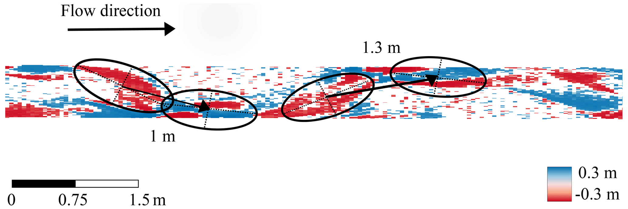
Figure 1Manual method to measure spacing of erosional patches (red) and depositional patches (blue) on a DoD.
2.2 Semiautomated extraction of path length
To visualize and then quantify the periodic nature of erosion and deposition from the DoD we simplify the spatial heterogeneity of the DoD into a vector of the net change in elevation in a streamwise direction (Fig. 2a). Because natural rivers are rarely straight, for field case studies, we must enforce a linear downstream directionality, essentially straightening the bends in the river. This is achieved by segmenting the DoD into a series of equally sized “bins” using the segmentation tool of the Fluvial Corridor Toolbox (Roux et al., 2015) (Fig. 2a). The bin size can affect the pattern of erosion and deposition in that by selecting bins that are too large we may miss important erosional or depositional areas when they are summed in the same bin. Similar methods that require river segmentation have proposed using the reach-averaged width for the length of the bins (McDowell et al., 2021) or half of the width of the reach (McDowell and Hassan, 2020), although these studies had different objectives. Calle et al. (2020) applied a segmentation method with a similar goal of identifying corresponding zones of erosion and deposition and set the bin size based on an assessment of the river dimensions as well as the minimum transfer distance of interest. Therefore, depending on the river, the user may select differently sized bins. Once the river is segmented, we then sum the values in each bin to obtain a vector of the net change in elevation in a downstream direction (Fig. 2b). In the flume studies, where there is no sinuosity, we simply sum each cross section of the DoD matrix. Oftentimes a reach is aggrading or incising, and therefore the net vector will have an increasing or decreasing trend (Fig. 2b). Because we are interested in the spacing between areas of erosion and deposition rather than the overall trend, we remove it by subtracting a best-fit linear trend from the net vector (Fig. 2b). Because we simplify the heterogeneity of erosion and deposition into a net vector of elevation change, we risk compensating for erosion and deposition within the same cross section; therefore, we also create a vector of just erosion and one of just deposition as well as the net, allowing for a visual comparison of the relative contribution of erosion and deposition to the net as well as the periodicity of the individual processes (Fig. A1). We can see that there appears to be a periodicity as the net vector oscillates, forming peaks and troughs, and although this periodicity seems apparent, quantifying the distance is not straightforward.
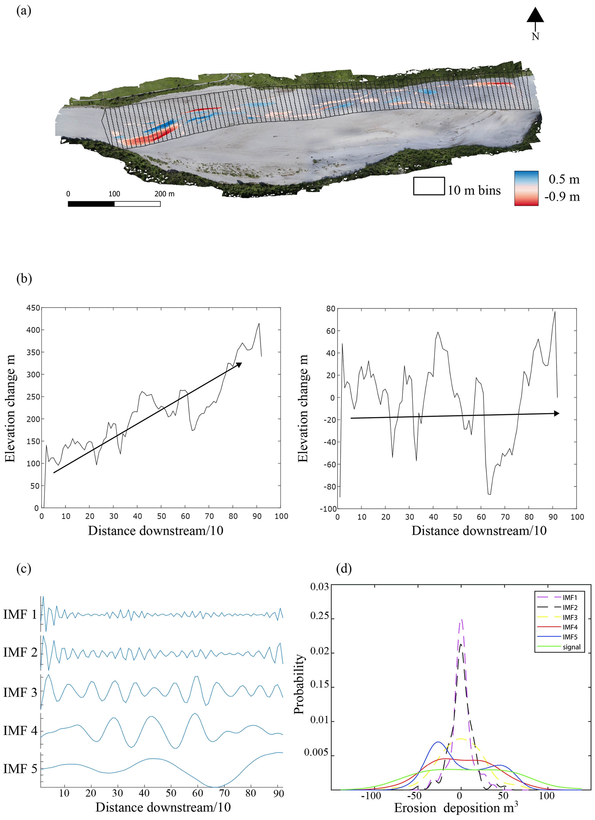
Figure 2VMD-HD method. (a) Segmentation of the DoD (example orthophoto and DoD from the Tagliamento River, Italy). (b) Plot of the net original and detrended vector. (c) Variational mode decomposition (VMD) with five intrinsic mode functions (IMFs). (d) Probability density function (PDF) of each IMF and the original net vector.
One approach could be to count the zero crossings and then use that distance as the proxy for path length. However, we risk measuring low-magnitude spikes that cross zero that may not necessarily represent the overall periodicity or large oscillations that do not cross the zero line. A smoothing filter may be used to remove these low-magnitude oscillations, but we risk losing potentially relevant information. To solve this problem, we turn to the realm of signal processing where the practice of “denoising” and extracting information from oscillations is ubiquitous.
Signal processing is a field that deals regularly with extracting information and patterns that are not visually apparent, and its applications have been used in a wide variety of settings including voice recognition (Sigmund, 2003; Upadhyay and Pachori, 2015), medical applications (Boudraa et al., 2005; Liu et al., 2008), and even time series analysis of climate data (Barnhart and Eichinger, 2011). There are many approaches to denoising including fast Fourier transform, empirical mode decomposition (EMD), and wavelet analysis. Each of these methods comes with inherent strengths and weaknesses; for example, wavelet analysis requires that a mother wavelet be selected a priori and may influence the results (Boudraa et al., 2005). We chose to use variational mode decomposition (VMD) due to its robustness with respect to sampling and noise and the ability to handle signals that exhibit nonlinearity and nonstationarity (Dragomiretskiy and Zosso, 2014; Huang et al., 2016; Ma et al., 2017). VMD decomposes the signal into a set of intrinsic mode functions (IMFs), each with a different central frequency (Dragomiretskiy and Zosso, 2014; Ma et al., 2017) (Fig. 2c). In the case of our static “signal” the frequency is more accurately described as the wavelength. It is beyond the scope of this paper to describe the mathematics of VMD in detail; therefore, for a complete explanation, see Dragomiretskiy and Zosso (2014), Huang et al. (2016), Ma et al. (2017), or Upadhyay and Pachori (2015).
Once the original net vector of erosion and deposition is decomposed into the various IMFs, we need to select the IMF(s) that most accurately represent the periodicity of the original data and therefore our characteristic path length. Ma et al. (2017) proposed a method to select the most relevant IMF and therefore periodicity of the signal by computing the probability density function (PDF) using kernel density smoothing for each of the five IMFs and of the original data vector (Fig. 2d), then calculate the Hausdorff distance (HD), a metric of geometric similarity, between each IMF's PDF and the PDF of the original data and select the IMF most geometrically similar to the original data (Ma et al., 2017) (hereafter the VMD-HD method). In most cases, the longer-wavelength IMFs most closely resemble the original signal, whereas the IMFs with shorter wavelengths are more likely associated with noise (Boudraa et al., 2005). The computed wavelength is converted to a meaningful physical quantity by multiplying by the bin spacing in meters. Because we are interested in the distance from peak to trough, we divide the period by 2 to obtain the path length proxy (Neill, 1971; Ashmore and Church, 1998). Although this method allows for the selection of one IMF to presumably represent the periodicity of the data, we record path lengths calculated from the other IMFs to evaluate the range of estimates generated by the decomposition and determine if the VMD-HD method is appropriate for determining a characteristic path length and the relative importance of other IMFs. All calculations were performed in MATLABR2020b using the built-in VMD function and the Hausdorff distance function (Danziger, 2023).
One important consideration when using VMD to decompose a signal is that is the user must define the number of IMFs beforehand. The number of IMFs is important as under-binning, or choosing too few IMFs, may mean that critical IMFs are missed, whereas over-binning can cause duplication of components (Wu et al., 2020). In signal processing, there are sophisticated methods for determining the number of IMFs; for a summary see Wu et al. (2020). However, for our purposes and simplicity's sake, we performed a brief sensitivity analysis based on the property of convergence often used in signal processing methods (Wu et al., 2020; Huang et al., 2016; Ma et al., 2017). The default setting in the MATLAB function is 5 IMFs, so we used 3, 5, 8, 15, and 25 IMFs to calculate path length and assessed how it changed for the maximum IMF (Fig. A2). We found that using more IMFs generally increased the number of high-frequency components rather than the lower-frequency IMFs (Fig. A3). Because these higher frequencies are generally associated with noise and in our case are physically too small to likely represent meaningful path lengths (on the order of millimeters) we decided that more than five IMFs did not contribute physically meaningful information in that the IMFs with longer wavelengths did not change drastically. We also determined that three IMFs were too few as it was clear that the longer wavelengths were missing (Fig. A3). Therefore, we chose to use the default five IMFs as this provided a manageable number of components while effectively separating the lower frequencies. This is a convenient starting point for assessing the VMD method as a tool to extract the periodicity as a proxy for characteristic path length but is by no means the only option. We encourage further exploration of the IMF parameter in future applications and as the method is refined.
The method was tested using data from a set of flume runs performed in the Hydraulic Laboratory of the University of Trento, where DEMs were generated for fixed time intervals and varying discharges, and direct measurements of the bedload flux were also collected. To test the efficacy of the method in the field, we selected a published dataset of measured path lengths with corresponding DoDs for the San Juan River in British Columbia, Canada (McQueen et al., 2021). Although McQueen et al. deployed tracers in four separate periods, there was only one deployment (2018–2019) with corresponding DEMs (McQueen et al., 2021). DoDs and corresponding tracer data were available for three separate sites (bar 6, bar 7, and bar 15) for the 2018–2019 period. Detailed information on their collection and processing can be found in McQueen et al. (2021).
3.1 Flume experiments
The Trento laboratory experiments were carried out in a 0.6 m wide and 24 m long flume, filled with nearly uniform 1 mm diameter sand. The flume slope was set to 0.01 m m−1. Topographic surveys were performed over the final 14 m of the flume to limit the upstream inflow effects using a laser gauge mounted on a movable deck. The longitudinal and crosswise spacings were 0.05 and 0.005 m, respectively. Four sets of nine runs were performed, with the flow discharge set to 0.7, 1, 1.5, and 2 L s−1, which correspond to a range of different planform morphologies (Table 1). Sediment input at the upstream end of the flume was constant in each run, with a flux equal to the average measured at the downstream end, as computed in a preliminary set of experiments. Therefore, the overall average bed elevation of the runs was in equilibrium, with no net erosion or deposition. The runs were performed following the same procedure, involving three phases of different lengths based on the transport condition of each discharge. These durations were estimated by referring to the timescale for morphological evolution computed from the sediment balance mass equation (Garcia Lugo et al., 2015), which can be expressed as
where D is the average flow depth and W is the flow width. Table 1 provides the values of T_ex for each flume experiment.
Table 1Initial conditions for each dataset including the type of validation data.
First, an initial phase of about 12 times this timescale T_ex with constant flow was run to ensure the formation of a near-equilibrium morphological condition, starting from a flat sand bed scraped to the prescribed slope. This was followed by a long run at constant discharge lasting 19 times the timescale T_ex, aimed at measuring the output sediment flux. This was continuously monitored at the channel outlet through a permeable basket placed on four load cells. Sediment flux was measured every minute. After a bed topography survey, the third phase was a sequence of nine shorter runs lasting 0.5 times the timescale T_ex, each followed by a bed topography survey, which produced nine corresponding DoDs. The duration of these nine runs (and therefore the time interval between surveys) was decided to have easily measurable changes in the bed morphology, without having significant compensation processes.
The DoDs were created by subtracting two consecutive DEMs, then underwent a three-step filtering process to highlight the relevant erosion and deposition patterns, removing most of the noise associated with the surface roughness and measurement accuracy. First, the DoDs were filtered considering a uniform detection threshold equal to 2 mm (2 times the D50), meaning that erosion or deposition values lower than this threshold are set to zero. Thereafter, a spatial average was performed as a moving average on three values along the transversal direction where the DoD discretization is the finest. Lastly, a despeckling algorithm removed all isolated cells considering both single cells that show erosion or deposition and single cells that show no change. This last step was implemented to keep the detection threshold as low as possible while removing unphysically small areas. Additionally, we calculated the morphological active width by determining the percentage of the DoD that showed morphological activity (i.e., was not zero after filtering).
3.2 San Juan River data
To compare the characteristic path length to measured path length distributions in the field, we used data from the San Juan River, located on Vancouver Island, British Columbia, with a drainage area of approximately 730 km2 and a mainly rainfall-driven hydrology (McQueen et al., 2021). The reach of interest in this study was alluvial in nature with a wandering morphology and a substrate composed of gravel, cobble, and sand (McQueen et al., 2021). The time between acquisitions is 1 year, during which it is estimated there were five flood events able to generate sediment transport using a threshold of 500 m3 s−1, which was visually estimated by the authors to be equivalent to the bankfull discharge (McQueen et al., 2021). DEMs were generated by lidar acquisitions and have a spatial resolution of 10 cm and a vertical root mean square error lower than 10 cm. Topographic changes between survey dates were then calculated by processing the lidar DEMs using the Geomorphic Change Detection (GCD) software (Wheaton et al., 2010). More information on how they were obtained and processed including the spatially variable thresholding techniques can be found in McQueen et al. (2021). The lidar-derived DoDs were used to interpret patterns of tracer displacement and burial depths and to provide information on the morphological development of the bars during the study period. However, they do not provide complete reach-scale sediment budgets due to the lack of in-channel topographic data and stage differences during each lidar survey affecting the relative portion of the riverbed that was exposed. The submerged area represented 22 % of the DoD for bar 6, 42 % for bar 7, and 36 % for bar 15. Nevertheless, we believe the exposed part of the channel, the bars, and associated patches of erosion and deposition (see Fig. 9b) are sufficient to be used with our proposed method to estimate path lengths and be compared with field-measured path lengths from the tracer data as a first application to field data. This is because we are not calculating sediment flux for the San Juan River and are only interested in comparing our estimates of the characteristic path length to the measured tracer distributions. As far as the pattern of erosion and deposition and how that may be disrupted, we recognize that the pattern could change by including the underwater areas; however, looking at Figs. 15 and 16 from McQueen et al. (2021) we can see that the tracers were largely recovered from the exposed bar surfaces in the 2018–2019 deployment. This gives us confidence that the deposition we are measuring corresponds largely to the deposition associated with the tracers. Although this is not an ideal situation, we believe the benefits outweigh the limitations considering the difficulty of finding high-quality RFID tracer data and corresponding DoDs. The San Juan River DoDs were downloaded directly from the Scholars Portal Dataverse (https://doi.org/10.5683/SP2/UQGZCG). The DoDs were segmented using similar principles to Calle et al. (2020) in a similarly sized river; therefore, the bin size was conservatively set at 10 m.
3.3 Validation and error estimation
Each study had unique initial conditions including slope, discharge, grain size, channel configurations, and time and flood events between surveys (Table 1). Because the studies vary with respect to these initial conditions, we calculated the dimensionless stream power (ω*) after Bertoldi et al. (2009) to compare them as
where Q is the peak discharge, S is slope, W is the average wetted width, Δ is the relative submerged density, D50 is the median grain size, and g is the acceleration due to gravity.
For the flumes, we used estimates of path length generated by the VMD-HD method and those associated with the two longest wavelengths, IMF 4 and IMF 5, separately to calculate the virtual velocity in Eq. (2) and sediment flux in Eq. (3), which we then compared to measured flux data. The measured sediment flux during the initial long run showed high variability, with phases of high and low sediment flux lasting several tens of minutes. For this reason, we prefer to use the data from the long runs, from which we estimated an average sediment flux of 0.33 g s−1 (SD = 0.17) for the 0.7 L s−1 discharge, 0.78 g s−1 (SD = 0.31) for the 1 L s−1 discharge, 1.98 g s−1 (SD = 0.65) for the 1.5 L s−1 discharge, and 3.22 g s−1 (SD = 0.79) for the 2 L s−1 discharge. We subdivided the second phase into 38 intervals of 0.5 T_ex duration, equal to the duration of the short runs in phase 3, and computed the variability of the flux over this range.
We used ANOVA to compare path length, virtual velocity, and erosion across the four discharges (α= 0.05) and a post hoc Tukey test to explore significant differences between discharges. To compare the measured sediment flux to the estimates from the VMD-HD method and the IMF 4 and IMF 5 estimates we used a Student's t test (α= 0.05). And finally, to compare the error of our path length and sediment transport estimates we calculated the relative percent error δ in order to compare the sediment flux estimates to that of the long runs of average sediment flux as
where E is the average of the estimated sediment flux for the nine runs at a given discharge and M is the averaged measured sediment flux from the long run at the same given discharge. For the San Juan River we compared the VMD-HD estimates of path length and IMFs 4 and 5 qualitatively to the published path length distributions and the locations of mean, median, and modes. The tracer recovery locations were accessed in spreadsheet form, and in keeping with the analysis of the authors we disregarded any tracers that moved less than 10 m before calculating the path length distributions.
4.1 Flume experiment
To aid in the interpretation of the results, Fig. 3 shows a DoD from the lowest discharge of 0.7 L s−1 (Fig. 3a) and the highest discharge of 2 L s−1 (Fig. 3b) with the net vector (continuous line), IMF 4 (dashed line), and IMF 5 (dotted line) as obtained from the VMD method. Oftentimes the areas of deposition and erosion from the DoD clearly correspond to the IMF 4 and 5 vectors as with the 0.7 L s−1 discharge where areas of deposition are concave and areas of net erosion correspond to convex areas of the vector (Fig. 3a). At the higher discharges (1.5 and 2 L s−1) the total area of morphological activity increases and patches of erosion and deposition begin to overlap, creating a more chaotic and difficult to discern pattern (Figs. 3b, A1). We also observed a similar periodicity in the erosional and depositional vectors, and at the 2 L s−1 discharge the depositional vector appears to show this most clearly (Fig. A1).
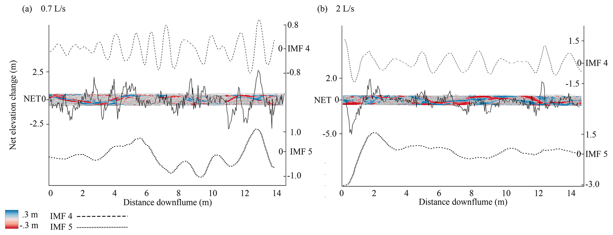
Figure 3DoDs from 0.7 L s−1 discharge (a) and 2 L s−1 discharge (b) with the net vector of elevation change laid over the top. IMF 4 vector (above, dashed line) and IMF 5 vector (below, dotted line).
In the flume experiment, the VMD-HD method of choosing the most relevant IMF selected the longest-wavelength IMF 5 71 % of the time and IMF 4 23 % of the time. IMFs 2 and 3 were never selected and IMF 1 was selected only twice. However, at the higher discharges (1.5 and 2 L s−1) IMF 4 was selected more frequently, thereby reducing the average path length when compared to the lower discharges (Fig. A4). Using the selected IMFs, the VMD-HD method estimated a similar average path length for all of the discharges (Fig. 4). The averages were 1.45 m (standard deviation (SD) = 0.93) for the 0.7 L s−1 discharge runs, 1.24 m (SD = 0.58) for the 1 L s−1 runs, 1.21 m (SD = 0.58) for the 1.5 L s−1 runs, and 1 m (SD = 0.37) for the 2 L s−1 runs (Fig. 4). The path length estimates derived from IMF 4 were similar for all discharges: 0.51 m (SD = 0.12) for the 0.7 L s−1 discharge, 0.55 m (SD = 0.16) for the 1 L s−1 discharge, 0.56 m (SD = 0.91) at the 1.5 L s−1 discharge, and 0.46 m (SD = 0.15) at 2 L s−1 (Fig. 4) with no significant differences between the discharges (p> 0.05). The path lengths derived from IMF 5 were also similar between the discharges with no significant differences (p> 0.05) and were 1.75 m (SD = 0.79) for the 0.7 L s−1 discharge, 1.55 m (SD = 0.24) for the 1 L s−1 discharge, 1.79 m (SD = 0.67) for the 1.5 L s−1 discharge, and 1.37 m (SD = 0.39) for the 2 L s−1 discharge (Fig. 4). The VMD-HD method closely matched the manually measured distances and there were no statistically significant differences for any of the discharges (p value > 0.05) (Fig. 4), while the IMF 4 and IMF 5 derived path lengths bracket the manually measured distances and the VMD-HD selected path lengths (Fig. 4).
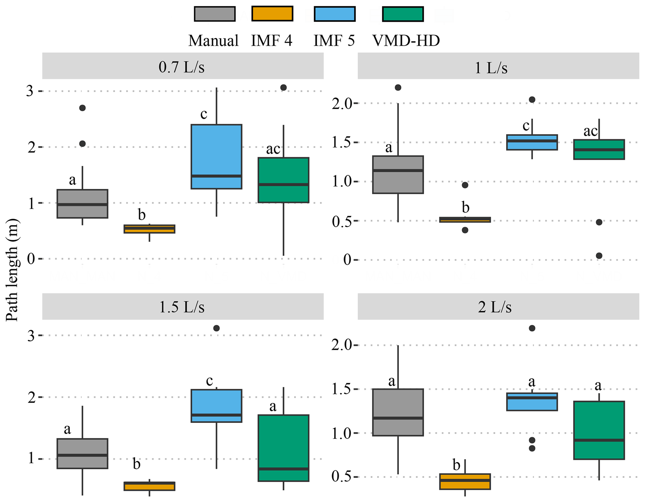
Figure 4Path length estimates from the manual method (gray), IMF 4 (orange), IMF 5 (blue), and the VMD-HD method (green). Significant differences from the post hoc Tukey test are denoted by letters a–c.
The estimated path lengths were not significantly different between the discharges (p value > 0.05) and showed no obvious trend of increasing or decreasing with discharge. However, when used to calculate the virtual velocity (vb) wherein the path length is divided by the time between surveys (Table 1), we see an increase in the virtual velocity with discharge (p value < 0.05) (Fig. 5). Likewise, the average volumes of erosion and deposition calculated from the filtered DoDs increase significantly with discharge (p value < 0.001) (Fig. 5).

Figure 5Estimated virtual velocity using the VMD-HD path length estimates, measured volumes of erosion, and deposition for each discharge. Significant differences from the post hoc Tukey test are denoted by letters a–c.
When used to calculate sediment transport in Eq. (3) the VMD-HD method corresponds well to the measured average for the lower discharges (0.7 and 1 L s−1) whereas at the higher discharges (1.5 and 2 L s−1) the method significantly underestimated the measured flux (Fig. 6). For the 0.7 L s−1 discharge, the VMD-HD method estimated a rate of 0.39 g s−1 (SD = 0.25) averaged over the nine runs, which was not significantly different than the measured average of 0.33 g s−1 (SD = 0.18), and the relative percent error (δ) was 18 %. For the 1 L s−1 discharge the method estimated 0.81 g s−1 (SD = 0.38) and was not significantly different than the measured average of 0.78 g s−1 (SD = 0.30, δ= 4 %). At the higher discharge of 1.5 L s−1 the average estimated by the VMD-HD method was 1.33 g s−1 (SD = 0.82), whereas the measured average was 1.98 g s−1 (SD = 0.70) (p value < 0.05, δ= 32 %). Finally, for the 2 L s−1 runs the estimated average was 1.41 g s−1 (SD = 0.48), whereas the measured average was 3.22 g s−1 (SD = 0.98) (p value < 0.001, δ= 56 %) (Fig. 6).
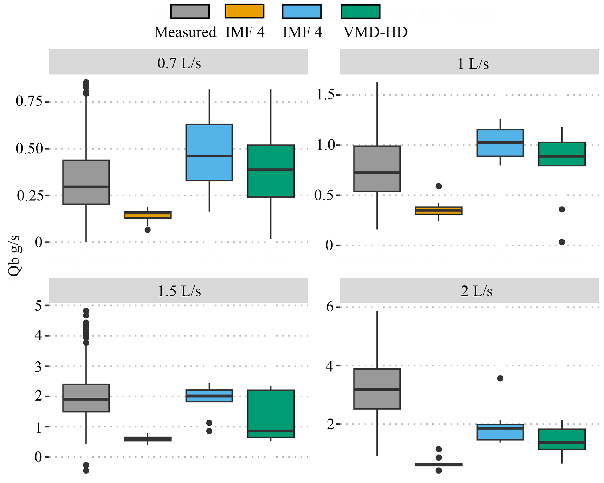
Figure 6Measured sediment flux (gray) compared to the estimates calculated using IMF 4 (orange), IMF 5 (blue), and the VMD-HD method (green). Significant differences from the post hoc Tukey test are denoted by letters a–c.
If we use just the IMF with the longest wavelength (IMF 5) to estimate path length and calculate sediment transport, we slightly overestimate sediment transport at the 0.7 L s−1 discharge as 0.48 g s−1, although not significantly (p> 0.05, δ= 45 %) (Fig. 6). At the 1 L s−1 discharge IMF 5 significantly overestimates the average flux with an estimate of 1.03 g s−1 (p<0.01, δ= 32 %). At the 1.5 L s−1 discharge the estimated flux of 1.88 g s−1 using the IMF 5 path lengths was not significantly different from the measured flux (p> 0.05, δ= 5 %) (Fig. 6). However, using the IMF 5 path lengths still significantly underestimated sediment flux at the 2 L s−1 discharge as 1.95 g s−1 (p<0.001, δ= 39 %) (Fig. 6).
Using the second-longest wavelength, IMF 4, we underestimate at all of the discharges (Fig. 6). The estimated flux was 0.14 g s−1 at the 0.7 L s−1 discharge (δ= 58 %), 0.36 g s−1 at the 1 L s−1 discharge (δ= 54 %), 0.61 g s−1 at the 1.5 L s−1 discharge (δ= 69 %), and 0.65 g s−1 at the 2 L s−1 discharge (δ= 80 %) (all p values < 0.001) (Fig. 6).
4.2 San Juan River
The 2018–2019 year for which we conducted our analyses was moderate in terms of excess flow energy with five flood events exceeding a discharge of 500 m3 s −1 and a peak discharge of 942 m3 s−1. The path length distributions of bar 7 and bar 15 are positively skewed, although there is a secondary mode in the bar 7 distribution roughly corresponding to the bar tail (Fig. 7), whereas the distribution of bar 6 is bimodal with the primary mode corresponding to the bar apex (Fig. 7). This is potentially because bar 6 had the most pronounced curvature, perhaps contributing to the clustering of deposition just before the apex, where a migrating gravel sheet terminated (McQueen et al., 2021). This bar apex corresponds to the path length from IMF 5 of 217 m, which was selected from the VMD-HD method (Fig. 7). IMF 5 was also selected by the VMD-HD method for bar 7, equaling 324 m, and here we see a correspondence to the small secondary mode where the authors note there was a clustering of tracers (Fig. 7) (McQueen et al., 2021). Again, IMF 5 with a path length of 323 m was also selected for bar 15 and closely corresponds to the bar apex, although there was not a clustering of tracer deposition in this deployment as observed in the year with higher discharge (Fig. 7). Additionally, bar 15 had the highest proportion of sand, which is not represented by the tracers, potentially contributing to the discrepancy between our estimates and the tracers. IMF 4 was always well below the lengths associated with the bar apexes and the median and mean tracer distances (Fig. 7). However, the bar apexes and the median and mean tracer distances were always between IMF 4 and IMF 5 (Fig. 7). The range between IMF 4 and IMF 5 accounted for 62 % of the path length distribution for bar 6, 36 % for bar 7, and 45 % for bar 15.
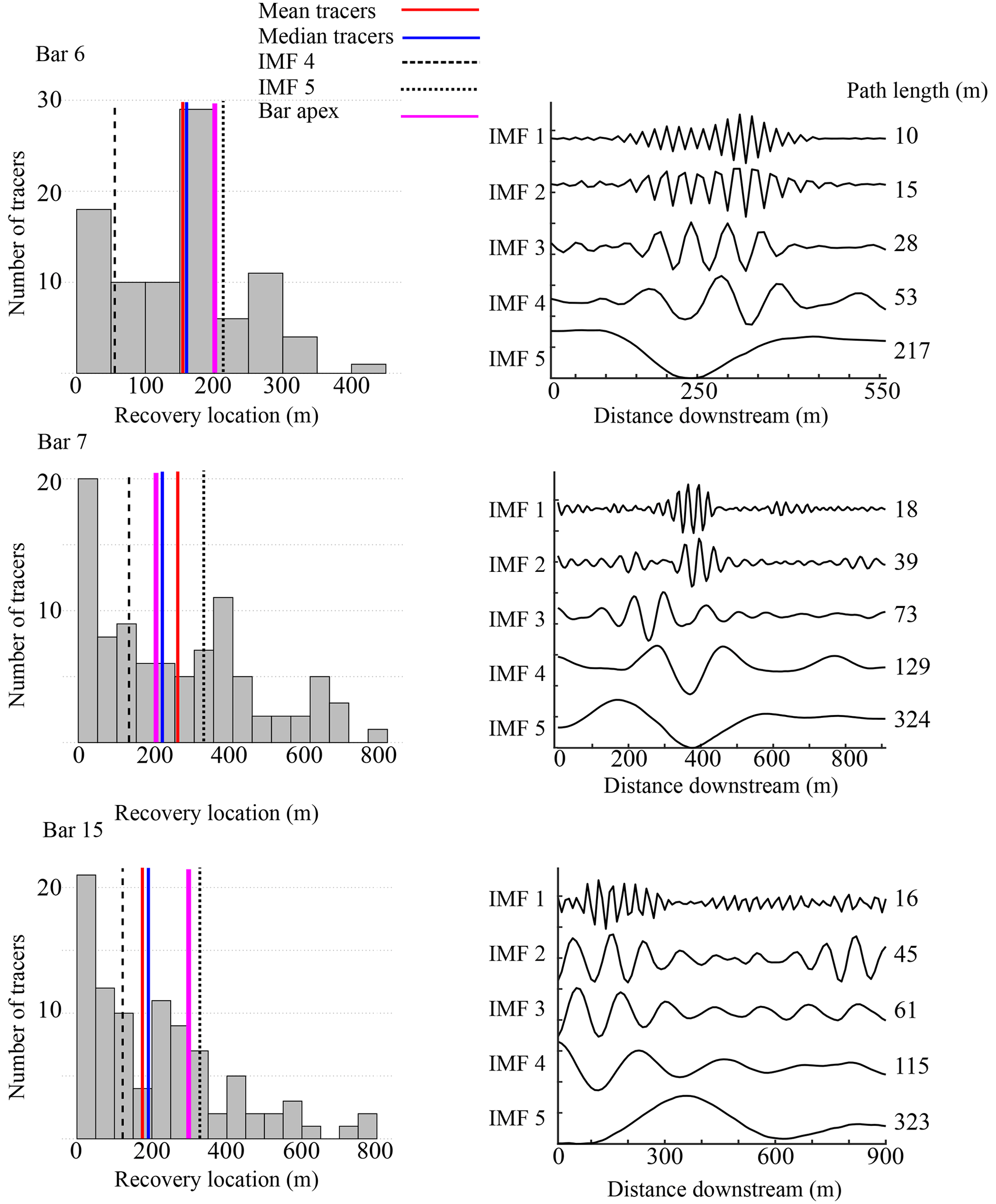
Figure 7Tracer-based path length distributions (on the left) and VMD-derived IMFs for bars 6, 7, and 15 from the San Juan River dataset. IMF 4 (dashed line), IMF 5 (dotted line), mean tracer distance (red), median tracer distance (blue), and the bar apex (pink) are shown over the path length distributions.
We developed a method to estimate the characteristic path length during a given flood using information inherent to the DoD by applying the principle that at channel-forming flows, the majority of particles move from an area of erosion to the next area of deposition downstream (Pyrce and Ashmore, 2003a, b). By using the periodic nature of erosion and deposition we overcome the subjectivity and time involved in measuring these distances manually while closely aligning with these manually measured distances (Fig. 4). When evaluating the efficacy of our proposed method it is important to keep in mind the uncertainty of even direct measurement of sediment transport. The spatial and temporal frequency required to overcome the noise of measurement uncertainty (i.e., achieve an acceptable signal-to-noise ratio) in some cases can require sub-daily monitoring with precise equipment (Grams et al., 2019). The variability of sediment transport measurements in the flume study ranged from a standard deviation of approximately 30 % to over 50 % of the averaged flux (Fig. 6). Given this high variability, our reach-scale averages were not significantly different from the measured averages for the 0.7 and 1 L s−1 discharges (Fig. 6). Importantly, we observed that the method underestimates the sediment flux significantly for the two highest discharges in the lab where the bed shows a higher percentage of the width experiencing topographic change (Fig. 6). The method presented to estimate a characteristic path length using only remotely sensed data shows promising results under certain conditions and provides insight into conditions where it is not applicable.
5.1 Path length estimation by VMD-HD method: limitations and perspectives
5.1.1 Flow effects
Previous studies have shown a relationship between path length and hydrologic variables such as discharge, stream power, and excess shear stress (Hassan et al., 1991; Pyrce and Ashmore, 2003b). A notable result of the flume experiment is that the estimated path length did not significantly differ between the four discharges (Fig. 5). We propose two possible explanations for this discrepancy with the literature. First, it is possible that the actual path length increases with discharge, as has been observed in previous studies (Hassan et al., 1991; Pyrce and Ashmore, 2003b), but the method fails to capture it because the VMD-HD method is based on the spacing of erosion and deposition, which does not change for the varying discharges under the flume conditions. It is possible that at higher discharges the characteristic path length, which we define as the distance from net erosional areas to net depositional areas, is not appropriate under the higher flow conditions because most particles are moving farther than the next depositional site downstream. This violates the assumption on which our method is based and is impossible to prove in our experiment without tracers. We can, however, look to the literature to understand the conditions in which tracers tend to travel more than one morphological unit (Liébault et al., 2012; Vázquez-Tarrío et al., 2019) and, coupled with future studies, perhaps determine the conditions under which a characteristic path length is inappropriate to estimate sediment transport.
From the San Juan River data we see that for a year with moderate flow, as characterized by the authors, very few tracers traveled further than the first depositional site downstream of their insertion point, although it is possible that the unrecovered tracers escaped the first bar. The recovery rates were high with 75 % of tracers recovered for bars 6 and 15 and 79 % recovered for bar 7 (McQueen et al., 2021). However, the moderate flow year for which we had corresponding tracer and DoD data resulted in two of the three sites having positively skewed distributions and only bar 6 showing a mode near the bar apex, which also corresponded to the IMF 5 path length (Fig. 7). The moderate flow conditions could explain why our estimates lined up more closely with the bar apex for bar 15, where in the previous high-flow year the majority of tracers were deposited, resulting in a symmetrical distribution (Fig. 8 from McQueen et al., 2021). It could be that our method is strongly influenced by the morphology of the channel such that when flow is insufficient to create symmetrical or bimodal path length distributions, we overestimate by using the characteristic path length because the majority of particles do not reach the next major depositional site downstream (i.e., a positively skewed distribution). Additionally, when the flow exceeds a yet unidentified threshold, the majority of particles move more than one depositional site downstream, and therefore we underestimate sediment transport by using the characteristic path length. We can speculate that this is happening to some extent in the flume experiment. We see that at the lowest discharge of 0.7 L s−1, we slightly overestimate the sediment flux, especially using IMF 5 (Fig. 6), and underestimate the flux at the highest discharge of 2 L s−1, where we also see a simplification of channel morphology (Figs. 6, 3). Because we did not have tracers in the flumes we cannot say if the path length distributions were in fact different between the lowest and highest discharges. Future applications of this method with tracer data in both the flumes and the field could help to understand when the characteristic length scale of morphology extracted by the method is an appropriate estimate of sediment transport and if this corresponds to flow metrics and path length distributions. In the flume studies we tested the idea that the majority of particles bypass the first depositional site simply by doubling the estimated path length. Assuming that sediment is not trapped in the first depositional area but in the second one and doubling the path length we more closely estimate the sediment transport at the higher discharges (i.e., estimates are not significantly different than the measured averages) (p>0.05) but overestimate the sediment transport at the 0.7 and 1 L s−1 discharges (p<0.05) (Fig. A5).
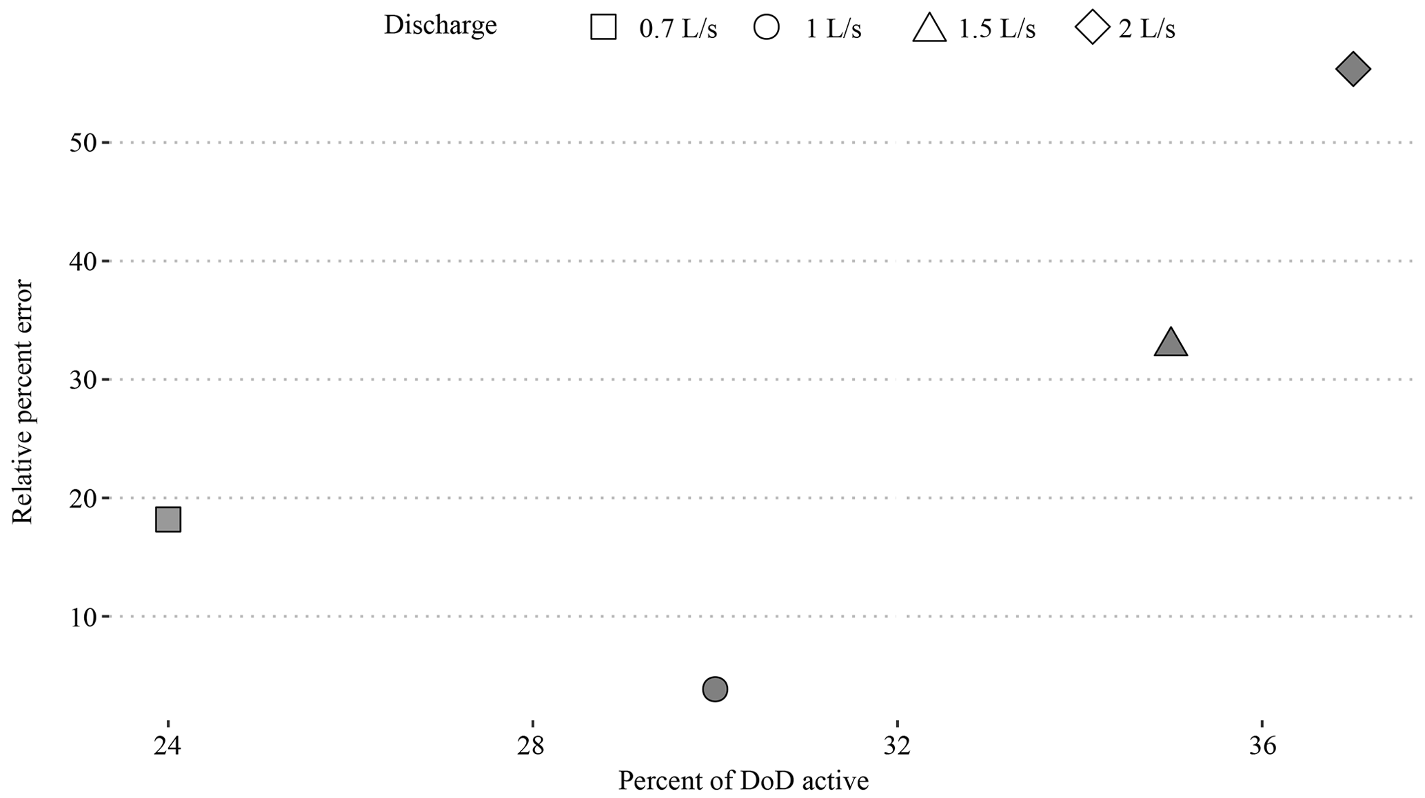
Figure 8Relative percent error between estimated flux using the VMD-HD method and the measured flux in the flume experiments (y axis) vs. the percentage of the DoD showing morphological change (x axis). Different discharges are denoted by shape.
5.1.2 Confinement
It is possible that due to the confined condition of the flumes, channel width may exert an outsized effect on the average bedload transport distance as the channel is unable to widen in response to an increase in discharge, thereby causing a flushing effect. In the flume experiment, we found that the VMD-HD method performed better at the lower discharges of 0.7 and 1 L s−1 but significantly underestimated the sediment transport at the 1.5 and 2 L s−1 discharges (Fig. 6). The underestimation at higher discharges could be related to the amount of morphological change relative to the sediment transport. Recently, Booker and Eaton (2022) quantitatively explored the link between sediment transport and morphology and proposed an index to represent the intuitive notion that as sediment transport increases relative to morphological change, the processes become decoupled and inferences from one to another become more difficult. They developed a “throughput index”, which is the ratio between sediment flux and morphological change and represents how much sediment moves through a reach without leaving a topographic signature of equal magnitude. Therefore, the ratio represents how well the flux is represented morphologically with the ratio approaching 1 when all of the flux is shown as morphological change and exceeding 1 when there is transport without equivalent morphological change. In our case the flume experiments were confined; therefore, as discharge increased the channel was not able to widen and deform laterally, potentially causing the sediment to move through the flume without leaving an equivalent topographic signature. To explore the applicability of the method proposed we calculated the morphological active width by counting the percentage of pixels in the DoD that showed topographic change after filtering (we applied this metric only for the flume experiments since the San Juan River DoDs do not include the submerged part of the channel). The morphological active width increased with discharge as expected and was positively correlated with the error of our estimates (Fig. 8). This result exposes a limitation of the morphological method in general and our application specifically: that is, confined channels with high transport relative to morphological change are likely poor candidates for the morphological method as inferences between changes in morphology and sediment transport become decoupled. Further applications of this method in the field and in the lab could identify a potential threshold defined by the throughput index (Booker and Eaton, 2022) or the morphological active width described in this study. The advantage of using the morphological active width as opposed to the throughput index is that it can be determined from the DoD without direct sediment transport measurements.
5.1.3 Morphological controls
Previous studies have shown that in gravel-bed rivers, macroform spacing is typically five to seven channel widths (Montgomery and Buffington, 1997), and therefore half of that spacing, i.e., pool to bar, may be considered a proxy for the characteristic path length. We compared our estimates of path length to (half of) both 5 and 7 times the channel width in the flumes and found that the IMF 5 estimates of path length were between the five and seven channel widths for all but the highest discharge (Fig. A6). Interestingly, the manually measured distances were less than the five to seven channel widths for all discharges but approaching five channel widths at the 2 L s−1 discharge (Fig. A6). When used to calculate sediment flux, the estimates derived from using five and seven channel widths were not significantly different than our VMD-HD estimates at discharges 0.7–1.5 L s−1 or the measured flux at all discharges (Fig. A5). Here we are likely seeing a good correspondence between the characteristic path length, width, and sediment transport because at formative discharges, morphology is the primary control on bedload travel distance, whereas at lower discharges, where the morphology is relatively stable, discharge may exert a stronger control on path length. Because we do not have tracer data in the flumes for comparison, we can only rely on the sediment transport measurements for validation, but further flume studies with both sediment flux and tracer data for validation could help resolve this question. The periodicity we extract from the DoDs as an estimate of path length corresponds to previous observations of preferential particle deposition at specific morphological units and relationships to channel morphology (Beechie, 2001; Pyrce and Ashmore, 2003a, b; Kasprak et al., 2015; McDowell and Hassan, 2020; McDowell et al., 2021). In the San Juan River study, our estimates closely aligned with the secondary modes in the particle path length distributions (Fig. 7), consistent with observations that at channel-forming flows, particle path lengths tend to be bimodal or multimodal, with secondary modes corresponding to the location of bars (Pyrce and Ashmore, 2003b). This preliminary result should be further examined with additional field data in multi-threaded channel types.
We expected that the path length in more complex channels such as braided configurations would be more difficult to estimate due to the possibility of multiple path lengths active at different flow stages. In this study both the flume experiment and the field study exhibited a wandering morphology, although in the flume experiment, the channel began to simplify at higher discharges, likely due to the inability of the channel to widen in response to the increase in discharge. Further, path length estimates did not change significantly between the discharges, whereas the erosion volume increases with discharge, and that, as mentioned previously, potentially contributed to the underestimation of sediment flux at the higher discharges. Additionally, at the 1.5 and 2 L s−1 discharges, the patches of erosion and deposition began to overlap; therefore, the wave-like pattern from areas of erosion to deposition represented by the IMF 5 vector became flattened (Figs. 3, A1). To disentangle the confounding erosion and deposition from the net vector, we applied the VMD method to a vector created from erosion and deposition separately. When calculating the path length using the erosion or deposition vectors, we took half of the resulting path length as we are still interested in the distance from erosion to deposition rather than erosion to erosion. We found that the path lengths generated from these vectors were not significantly different than the path lengths generated using the net vector (p> 0.05) (Fig. A6), nor were the estimates of sediment transport (Fig. A5) This evidence supports the use of the net vector in this case because it appears that erosion and deposition were similarly distributed. However, in rivers with differing morphology, perhaps braided systems, we might suspect that erosion will be more localized than deposition, which can be dispersed (Goff and Ashmore, 1994). In these cases, using VMD to decompose the net erosion and deposition separately could give further insight into how deposition and erosion contribute to the net change. For example, deposition may contribute little to the net vector if the relative magnitude of the oscillations is small compared to erosion, which tends to be more concentrated. In addition to estimating a characteristic path length, this decomposition could give further insight into the nature of depositional and erosional processes in a reach. We also recognize that perhaps when multiple channels are present and active, it may be beneficial to segregate the DoD, treating each channel as a separate system, and generate multiple path length estimations to avoid compensating for erosion and deposition within the cross section. Further investigations are needed in the lab and in the field to propose robust methodologies to assess realistic ranges of path lengths from DoDs for varying river patterns.
5.1.4 Using the IMFs
The path-length-based method for calculating sediment transport necessitates that a single path length be selected, and this is surely an oversimplification of reality. Encouragingly, the flume experiment shows that by using the VMD-HD method to select the path length, we are able to reasonably approximate sediment transport at the lower discharges (Fig. 6). However, when applying this method to a real case study, like that of the San Juan River, it is important to consider whether the results make sense given what is known about the channel as well as the time and magnitude of flood events between surveys, potentially taking into account both IMF 4 and IMF 5 to generate a range of plausible transport or path lengths. The VMD-HD method presented here selects one of the five IMFs to be used as an estimate of path length based on the geometric similarity, as measured by the Hausdorff distance, of the IMF to the original data vector. However, we presume that not only does the method occasionally select an erroneous IMF (IMF 1, for example, where the path length is on the order of millimeters) but also that in some cases more than one IMF could represent the pattern of erosion and deposition in the DoD or perhaps a range due to the heterogeneous nature of sediment transport. In the flume experiment, the VMD-HD method selected the longest wavelength, IMF 5, 74 % of the time and IMF 4 24 % of the time. There were only two instances in which IMF 1 was selected and neither IMF 2 nor 3 was ever selected. Likewise, IMF 5 was selected for all three bars in the San Juan River dataset. This result agrees with observations from the signal processing literature wherein the lower-frequency (in our case wavelength) IMFs (4 and 5) are thought to represent the true signal, whereas the higher-frequency (shorter-wavelength) IMFs are attributed to noise (Boudraa et al., 2005). In our case we can visually verify that IMF 5 is most likely representative of the characteristic path length by tracing the path from erosional site to depositional site within the DoD using the manual method (Fig. 9). Here we see that the longest IMF captures the spacing between erosional and depositional patches as estimated by other methods (Redolfi, 2014; Vericat et al., 2017; Calle et al., 2020). This study, as the others, supports the idea that the periodic nature of erosion and deposition can be used to estimate sediment transport and helps to clarify the conditions where this approach is valid. Moreover, this study provides an objective and repeatable method to estimate the characteristic path length.
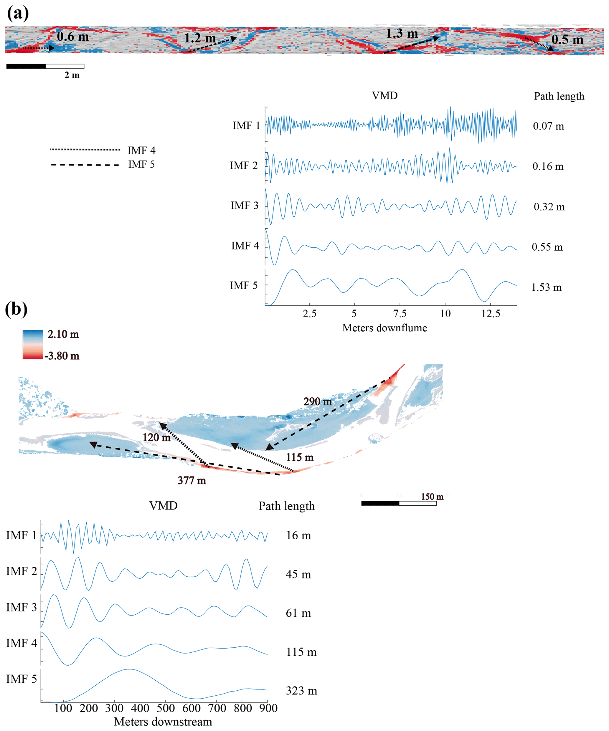
Figure 9DoD with arrows showing possible path lengths between areas of erosion (red) and deposition (blue) corresponding to both IMF 4 and IMF 5. The VMD breakdown including all IMFs and the corresponding path lengths are shown for an experimental run from the 1.5 L discharge (a) and bar 15 from the San Juan River (b).
Different IMFs also allow us to explore multiple periodicities, such as shorter path lengths in the DoDs that may correspond to IMF 4 (Fig. 9). The method we present here to select one of the IMFs to represent the periodicity is convenient for assigning a characteristic path length to be used in sediment transport calculations. However, it is unclear if the range of IMFs may be used to estimate aspects of the path length distribution. As a first step, we see that in the San Juan River the path lengths associated with IMF 4 and IMF 5 bracket the mean, median, and key depositional areas associated with the path length distribution (Fig. 7). With future studies it may be possible to set a range of plausible transport based on IMFs 4 and 5.
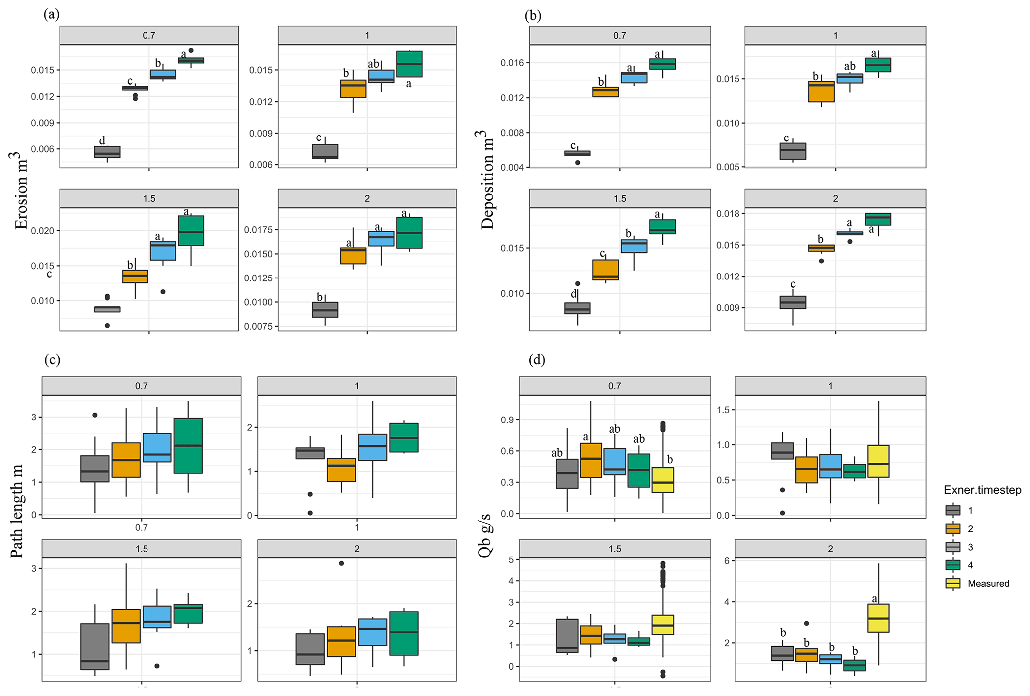
Figure 10(a) Erosion measured from the flume experiments for each discharge and each time step. (b) Deposition and (c) path length estimates using the VMD-HD method. (d) Sediment flux estimated using the VMD-HD method and measured. Significant post hoc Tukey results are denoted by letters a–d (α= 0.05).
5.2 DoD-related uncertainties
Any application of the morphological method using DoDs is sensitive to the error thresholding method used due to the way in which different thresholding techniques influence the volumes of erosion and deposition as well as their spatial patterning (Brasington et al., 2003; Wheaton, 2008; Wheaton et al., 2010; Vericat et al., 2017). Because our method relies on the spacing between areas of erosion and deposition, which is related to the size of the patches as well as which patches are detected, we considered that thresholding techniques could greatly affect the estimates of path length. We tested this hypothesis by applying the method to both the raw and filtered DoDs for the Trento flume experiment and found that while the volumes of erosion and deposition were lower after thresholding as expected (p<0.001), the path length estimates were not significantly different (p>0.05) (Table A1). While the thresholding here did not affect the path length estimates, we might imagine a scenario in which an entire area of erosion or deposition is removed through aggressive thresholding techniques, thereby potentially affecting the path length estimates; we therefore caution that appropriate thresholding is important for the application of this method and the morphological method in general. It is also important to consider the spatial resolution (i.e., raster cell size) of the DoD when applying this method. Similarly to thresholding or selecting a bin size, the spatial resolution of the DoD could cause information to be lost if the cell size is large enough to aggregate erosion and deposition within the same cell (see, for instance, the comparison made in Antoniazza et al., 2019). We see less of a risk in using smaller cell sizes as the method already calls for aggregation in the binning process, and in theory VMD should be able to separate the small-scale fluctuations as short-wavelength IMFs. However, this is an open question and should be evaluated by the user on a case-by-case basis.
The time between surveys is of equal importance to the path length in the estimation of virtual velocity and in the field can be highly uncertain due to poor availability of hydrologic data and/or the uncertainty of estimating the onset of transport based on a critical shear stress. Further, as the time between surveys increases, so does the probability of compensating for erosion and deposition, which can affect both the volumes of erosion and deposition and the topographic signatures (Lindsay and Ashmore, 2002; Vericat et al., 2017) necessary for the VMD-HD method. We tested how the time between surveys might affect the volumes of erosion and deposition as well as our path length estimates by differencing DEMs not every time step but between two, three, and four time steps, each time step being one of the nine runs in the lab of phase 3 (see the Methods section). Not surprisingly the volume of erosion and deposition increased significantly with increasing time between surveys, with the largest increase between the first time step and second time step (Fig. 10). The path length estimates did not increase significantly for any of the discharges (Fig. 10c), indicating that the path length estimate is stable, likely because, as already noted, the spacing of erosion and deposition is related to the position of erosional and depositional features, which do not change much in the flume. When both of these parameters are used in the sediment transport calculations and normalized by the increased time between surveys, we found no statistically significant difference between the estimates (Fig. 10d). However, though not statistically significant, there is an apparent decreasing trend in the sediment flux with increased time between surveys, especially for the 2 L s−1 discharge, that may indicate compensation (Fig. 10d). Despite the apparent trend at the highest discharge, this is a promising result in that even by increasing the time interval by a factor of 4 we are still able to estimate sediment transport reasonably at the lower discharges. In the field there are often multiple flood events of differing magnitude in the year between surveys, as was the case with the San Juan River study (McQueen et al., 2021). Although there were five flood events of differing magnitudes between the San Juan River surveys, we were still able to estimate path lengths corresponding to potentially significant features of the path length distributions (Fig. 7).
Given the observed connections between morphology and path length at channel-forming flows, we proposed that the periodic nature of the pattern of erosion and deposition can be a proxy for a characteristic path length in gravel-bed rivers. We applied tools from signal processing to quantify this periodicity and found that by the longest wavelengths from the decomposition, IMF 4 and IMF 5 may represent meaningful bedload transport processes, and IMF 5 in particular may represent the characteristic path length. We found that the path length estimates generated by IMFs 4 and 5 bracket a significant portion of measured path length distributions in the field and correspond to important morphological units. In the flume experiment we found that IMF 4 and 5 path lengths also bracket the manually measured distances between erosional and depositional patches, and when extended to calculate sediment flux our estimates were not significantly different from the measured average at low discharges. Importantly we found an insensitivity of the method to increasing discharge and propose that perhaps limits arise where discharge increases in confined settings, such as in the flume, and sediment transport becomes decoupled from morphological changes. Our method provides a new view of the periodic nature of erosion and deposition in sediment transport and a novel way to extract sediment transport information using only DoDs.
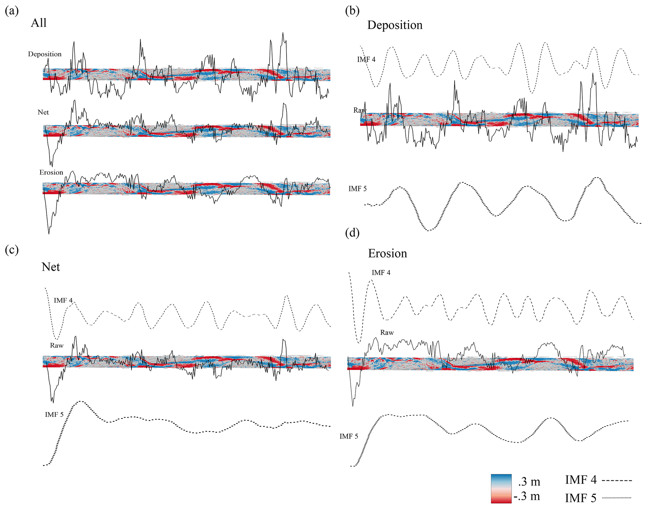
Figure A1DoDs from the 2 L s−1 discharge. (a) Vector of deposition, erosion, and net. (b) Raw depositional vector and the decomposition of IMF 4 and IMF 5 from that depositional vector. (c) Net vector and the decomposition of IMF 4 and IMF 5 from that net vector. (d) Raw erosional vector and the decomposition of IMF 4 and IMF 5 from that erosional vector.
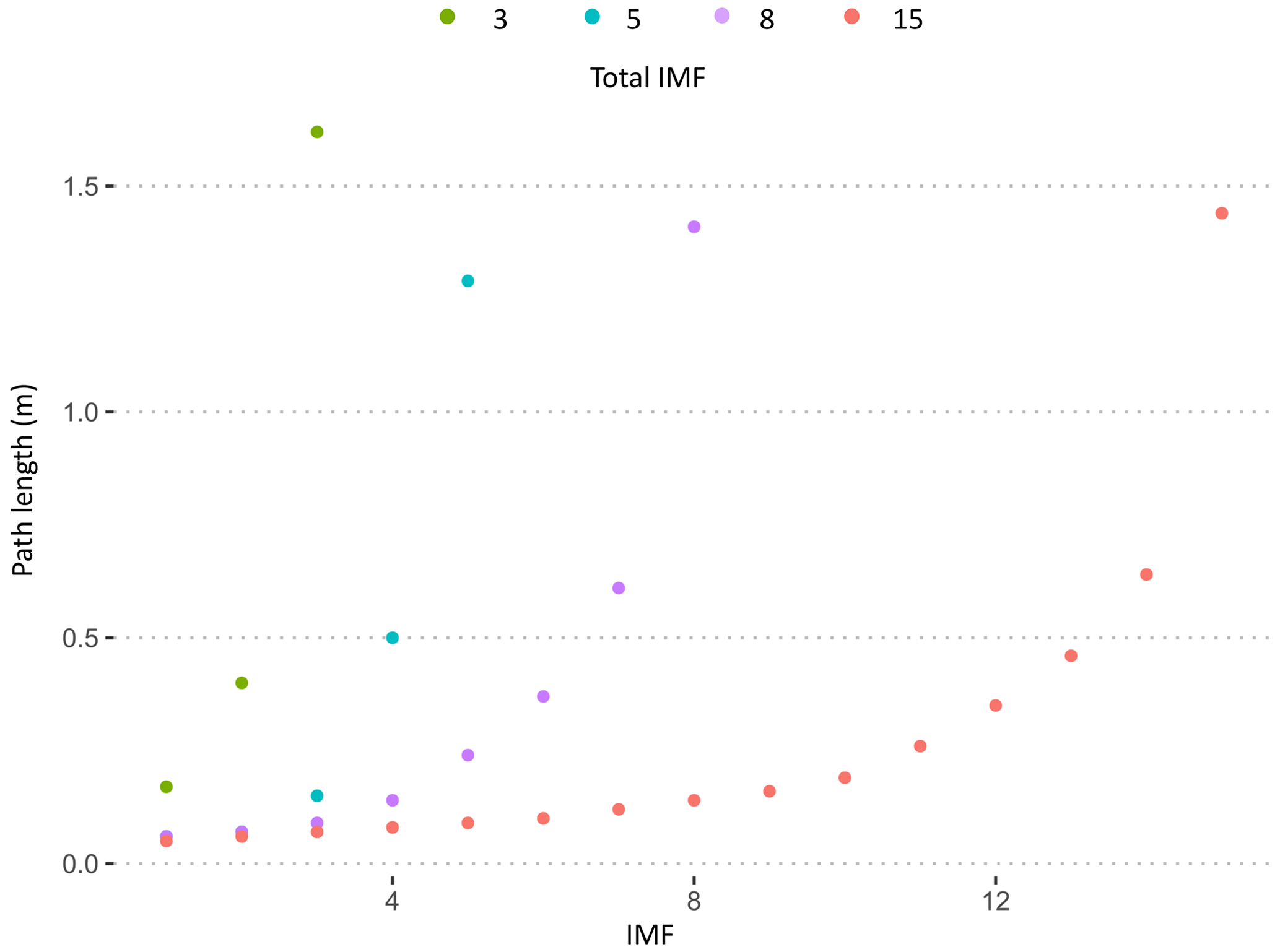
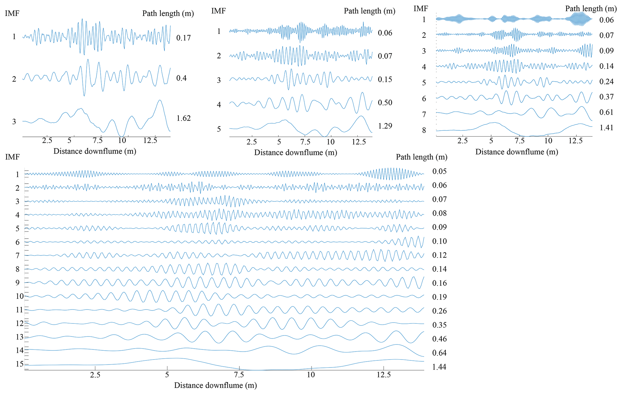
Figure A3Path length estimates from VMD for 1.5 L s−1 discharge. Sensitivity of maximum number of IMFs.
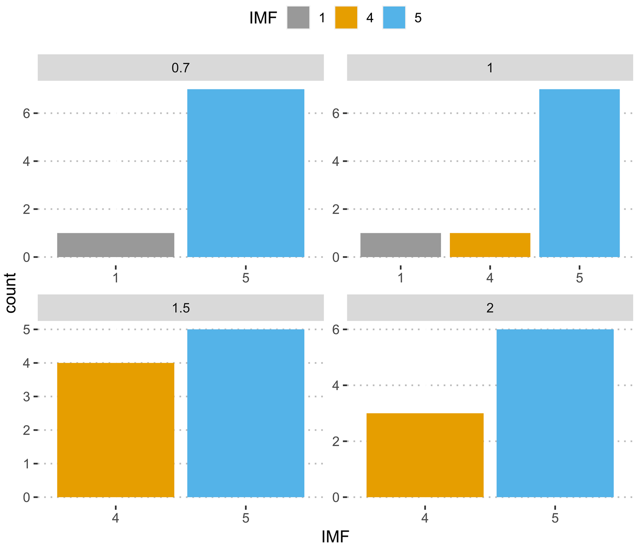
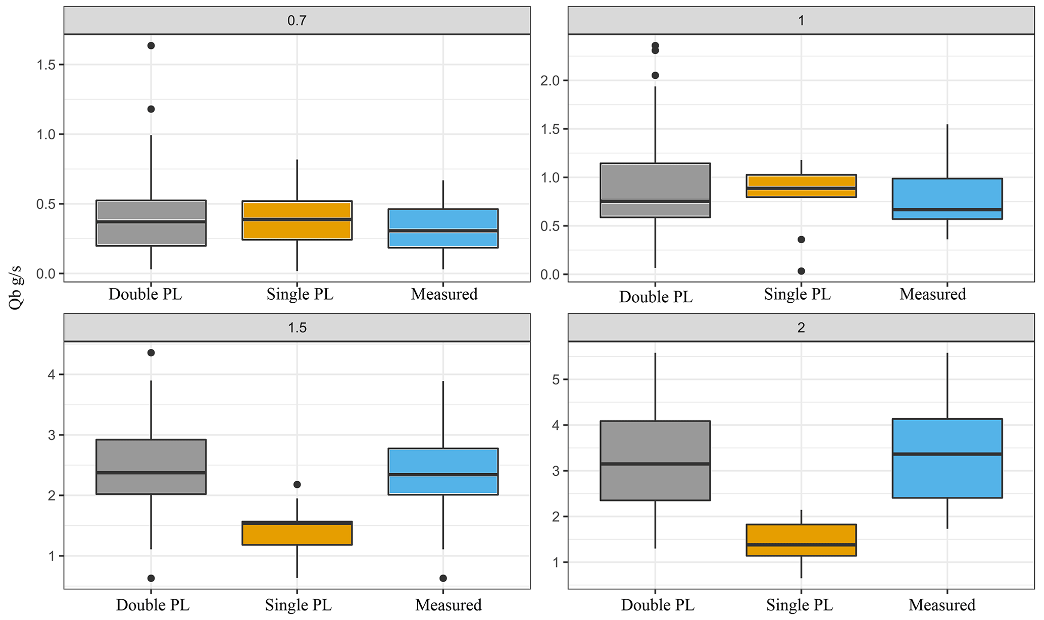
Figure A5Sediment transport calculated using the single path length estimate from the VMD-HD method (orange), doubling the path length estimate (gray), and the measured flux (blue).
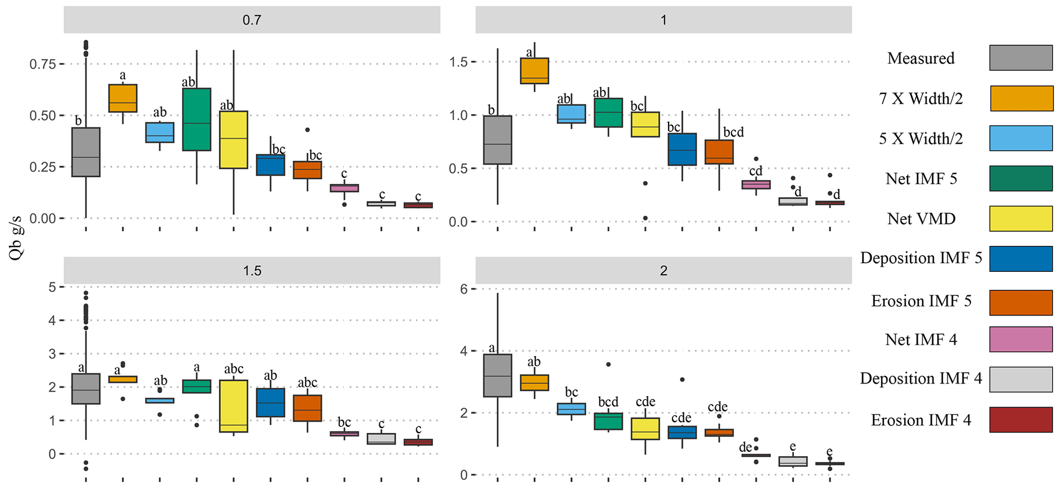
Figure A6Sediment transport (g s−1) calculated using channel dimensions, IMFs 4 and 5 for net erosion, and deposition vector compared to the measured flux for each discharge. Post hoc Tukey results are denoted by letters a–f.
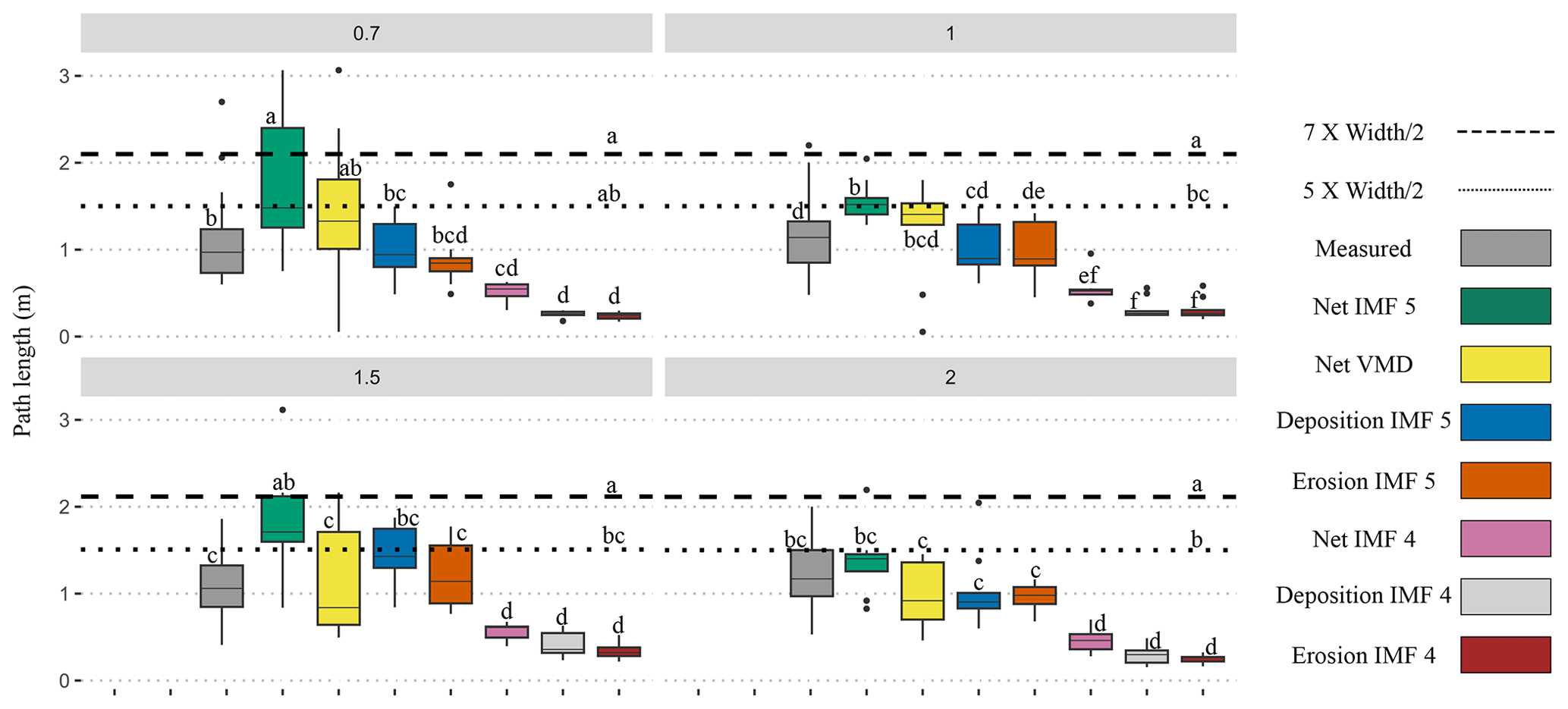
Figure A7Path length estimates from the channel dimensions, IMFs 4 and 5 for net, erosion, and deposition vectors compared to manually measured distances for each discharge. Post hoc Tukey results are denoted by letters a–f.
Table A1Results from filtered vs. raw DoDs from the flume experiments.
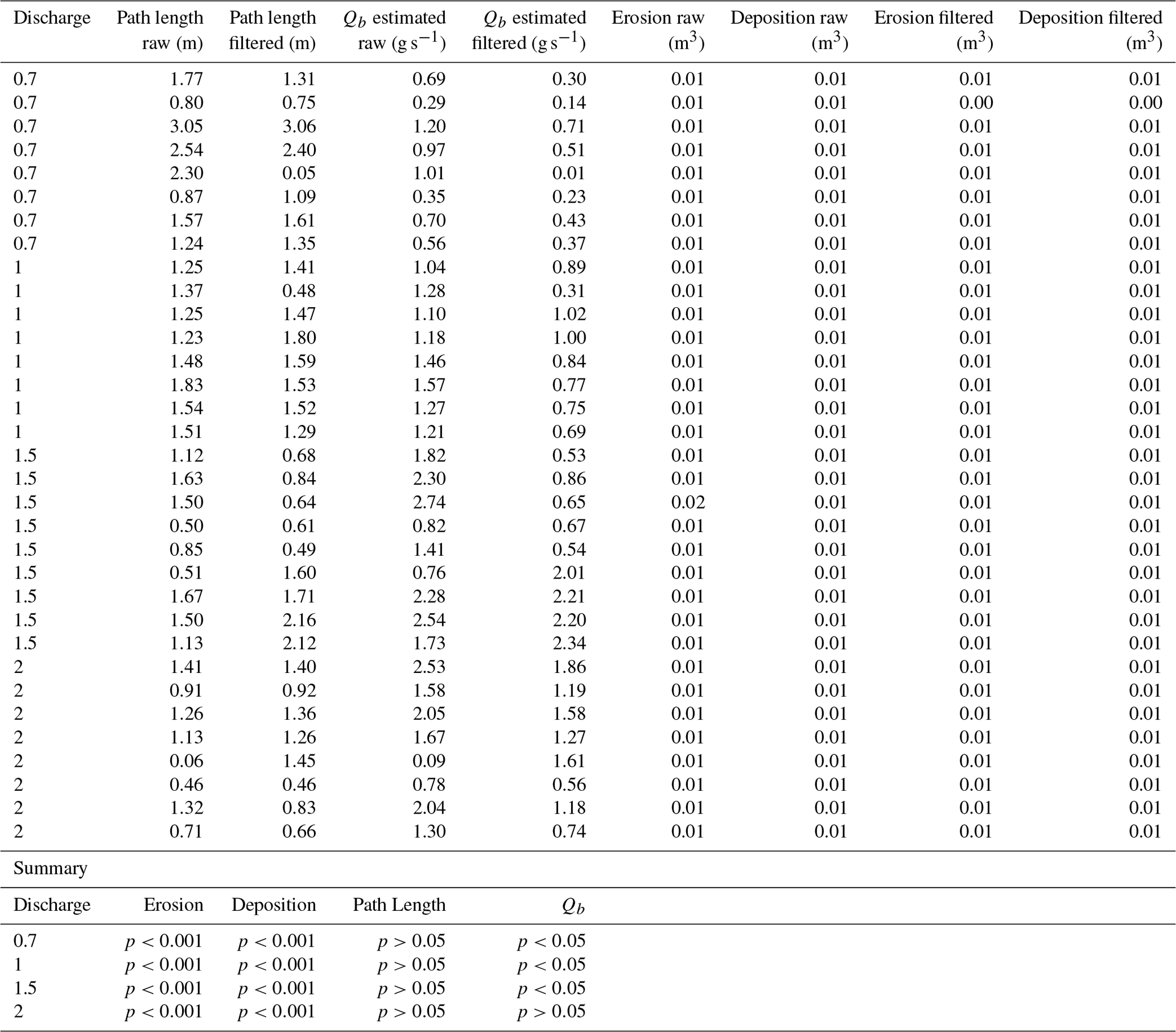
The p values from a Student's t test between raw and filtered data.
Data are available at https://doi.org/10.5281/zenodo.8014453 (Pandrin and Bertoldi, 2023).
LMC, SB, WB, and NS conceptualized the study. EP preformed the experiments. LMC, SB, and WB designed the method. LMC performed statistical analysis. LMC, EP, and WB wrote the paper. LMC, SB, EP, WB, and NS edited the paper.
The contact author has declared that none of the authors has any competing interests.
Publisher's note: Copernicus Publications remains neutral with regard to jurisdictional claims made in the text, published maps, institutional affiliations, or any other geographical representation in this paper. While Copernicus Publications makes every effort to include appropriate place names, the final responsibility lies with the authors.
We would like to thank the three anonymous referees for their time and thoughtful suggestions, which have considerably improved the quality of this work. We would also like to thank the CARIPARO foundation and the University of Padova.
This work was supported by the CARIPARO foundation and the University of Padova.
This paper was edited by Fiona Clubb and reviewed by three anonymous referees.
Antoniazza, G., Bakker, M., and Lane, S. N.: Revisiting the morphological method in two-dimensions to quantify bed-material transport in braided rivers, Earth Surf. Proc. Land., 44, 2251–2267, https://doi.org/10.1002/esp.4633, 2019.
Ashmore, P. E. and Church, M.: Sediment transport and river morphology: a paradigm for study, Gravel-Bed Rivers Environ., 345, 115–139, 1998.
Bakker, M., Antoniazza, G., Odermatt, E., and Lane, S. N.: Morphological Response of an Alpine Braided Reach to Sediment-Laden Flow Events, J. Geophys. Res.-Earth, 124, 1310–1328, https://doi.org/10.1029/2018JF004811, 2019.
Barnhart, B. L. and Eichinger, W. E.: Empirical Mode Decomposition applied to solar irradiance, global temperature, sunspot number, and CO2 concentration data, J. Atmos. Sol.-Terr. Phy., 73, 1771–1779, https://doi.org/10.1016/j.jastp.2011.04.012, 2011.
Beechie, T. J.: Empirical predictors of annual bed load travel distance, and implications for salmonid habitat restoration and protection, Earth Surf. Proc. Land., 26, 1025–1034, https://doi.org/10.1002/esp.251, 2001.
Bertoldi, W., Zanoni, L., and Tubino, M.: Planform dynamics of braided streams, Earth Surf. Proc. Land., 34, 547–557, https://doi.org/10.1002/esp.1755, 2009.
Booker, W. H. and Eaton, B. C.: Morphodynamic styles: characterising the behaviour of gravel-bed rivers using a novel, quantitative index, Earth Surf. Dynam., 10, 247–260, https://doi.org/10.5194/esurf-10-247-2022, 2022.
Boudraa, A.-O., Cexus, J.-C., and Saidi, Z.: EMD-Based Signal Noise Reduction, Signal Process., 1, 33–37, 2005.
Brasington, J., Rumsby, B. T., and McVey, R. A.: Monitoring and modelling morphological change in a braided gravel-bed river using high resolution GPS-based survey, Earth Surf. Proc. Land., 25, 973–990, https://doi.org/10.1002/1096-9837(200008)25:9<973::AID-ESP111>3.0.CO;2-Y, 2000.
Brasington, J., Langham, J., and Rumsby, B.: Methodological sensitivity of morphometric estimates of coarse fluvial sediment transport, Geomorphology, 53, 299–316, https://doi.org/10.1016/S0169-555X(02)00320-3, 2003.
Brenna, A. and Surian, N.: Coarse sediment mobility and fluxes in wide mountain streams: Insights using the virtual velocity approach, Geomorphology, 427, 108625, https://doi.org/10.1016/j.geomorph.2023.108625, 2023.
Brenna, A., Surian, N., and Mao, L.: Virtual Velocity Approach for Estimating Bed Material Transport in Gravel-Bed Rivers: Key Factors and Significance, Water Resour. Res., 55, 1651–1674, https://doi.org/10.1029/2018WR023556, 2019.
Brenna, A., Surian, N., Ghinassi, M., and Marchi, L.: Sediment–water flows in mountain streams: Recognition and classification based on field evidence, Geomorphology, 371, 107413, https://doi.org/10.1016/j.geomorph.2020.107413, 2020.
Brewer, P. A. and Passmore, D. G.: Sediment budgeting techniques in gravel-bed rivers, Geol. Soc. Lond. Spec. Publ., 191, 97–113, https://doi.org/10.1144/GSL.SP.2002.191.01.07, 2002.
Calle, M., Calle, J., Alho, P., and Benito, G.: Inferring sediment transfers and functional connectivity of rivers from repeat topographic surveys, Earth Surf. Proc. Land., 45, 681–693, https://doi.org/10.1002/esp.4765, 2020.
Church, M.: Bed Material Transport and the Morphology of Alluvial River Channels, Annu. Rev. Earth Pl. Sc., 34, 325–354, https://doi.org/10.1146/annurev.earth.33.092203.122721, 2006.
Church, M. and Haschenburger, J. K.: What is the “active layer”?, Water Resour. Res., 53, 5–10, https://doi.org/10.1002/2016WR019675, 2017.
Danziger, Z.: Hausdorff Distance, MATLAB Central File Exchange https://www.mathworks.com/matlabcentral/fileexchange/26738-hausdorff-distance (last access: 10 February 2023), 2023.
Dragomiretskiy, K. and Zosso, D.: Variational Mode Decomposition, IEEE T. Signal Proces., 62, 531–544, https://doi.org/10.1109/TSP.2013.2288675, 2014.
Einstein, H. A.: Bedload transport as a probability problem, PhD Dissertation, (English translation), in: Sedimentation, Water Resources Publications, edited by: Shen, H. W., Fort Collins, CO, Appendix C, 105 pp., 1937.
Ferguson, R. I. and Ashworth, P. J.: Spatial patterns of bedload transport and channel change in braided and near-braided rivers, Dyn. Gravel-Bed Rivers, edited by: Billi, P., Hey, R. D., Thorne, C. R., and Tacconi, P., https://www.researchgate.net/publication/279961017_Spatial_patterns_of_bedload_transport_and_channel_change_in_braided_and_near-braided_rivers (last access: 10 March 2023), 1992.
Garcia Lugo, G. A., Bertoldi, W., Henshaw, A. J., and Gurnell, A. M.: The effect of lateral confinement on gravel bed river morphology, Water Resour. Res., 51, 7145–7158, https://doi.org/10.1002/2015WR017081, 2015.
Goff, J. R. and Ashmore, P.: Gravel transport and morphological change in braided sunwapta river, Alberta, Canada, Earth Surf. Proc. Land., 19, 195–212, https://doi.org/10.1002/esp.3290190302, 1994.
Grams, P. E., Topping, D. J., Schmidt, J. C., Hazel Jr., J. E., and Kaplinski, M.: Linking morphodynamic response with sediment mass balance on the Colorado River in Marble Canyon: Issues of scale, geomorphic setting, and sampling design, J. Geophys. Res.-Earth, 118, 361–381, https://doi.org/10.1002/jgrf.20050, 2013.
Grams, P. E., Buscombe, D., Topping, D. J., Kaplinski, M., and Hazel, J. E.: How many measurements are required to construct an accurate sand budget in a large river? Insights from analyses of signal and noise, Earth Surf. Proc. Land., 44, 160–178, https://doi.org/10.1002/esp.4489, 2019.
Hassan, M. A. and Bradley, D. N.: Geomorphic Controls on Tracer Particle Dispersion in Gravel-Bed Rivers, in: Gravel-Bed Rivers, John Wiley & Sons Ltd., 159–184, https://doi.org/10.1002/9781118971437.ch6, 2017.
Hassan, M. A., Church, M., and Schick, A. P.: Distance of movement of coarse particles in gravel bed streams, Water Resour. Res., 27, 503–511, https://doi.org/10.1029/90WR02762, 1991.
Hassan, M. A., Church, M., and Ashworth, P. J.: Virtual rate and mean distance of travel of individual clasts in gravel-bed channels, Earth Surf. Proc. Land., 17, 617–627, https://doi.org/10.1002/esp.3290170607, 1992.
Hoey, T.: Temporal variations in bedload transport rates and sediment storage in gravel-bed rivers, Prog. Phys. Geog., 16, 319–338, https://doi.org/10.1177/030913339201600303, 1992.
Huang, N., Chen, H., Cai, G., Fang, L., and Wang, Y.: Mechanical Fault Diagnosis of High Voltage Circuit Breakers Based on Variational Mode Decomposition and Multi-Layer Classifier, Sensors, 16, 1887, https://doi.org/10.3390/s16111887, 2016.
Hundey, E. J. and Ashmore, P. E.: Length scale of braided river morphology, Water Resour. Res., 45, 1–9, https://doi.org/10.1029/2008WR007521, 2009.
Inc, T. M.: MATLAB version: 9.13.0 (R2022b), https://www.mathworks.com (last access: 1 January 2022), 2022.
Kasprak, A., Wheaton, J. M., Ashmore, P. E., Hensleigh, J. W., and Peirce, S.: The relationship between particle travel distance and channel morphology: results from physical models of braided rivers., J. Geophys. Res.-Earth, 120, 55–74, 2015.
Lane, S. N., Richards, K. S., and Chandler, J. H.: Morphological Estimation of the Time-Integrated Bed Load Transport Rate, Water Resour. Res., 31, 761–772, https://doi.org/10.1029/94WR01726, 1995.
Lane, S. N., Westaway, R. M., and Murray Hicks, D.: Estimation of erosion and deposition volumes in a large, gravel-bed, braided river using synoptic remote sensing, Earth Surf. Proc. Land., 28, 249–271, https://doi.org/10.1002/esp.483, 2003.
Liébault, F., Bellot, H., Chapuis, M., Klotz, S., and Deschâtres, M.: Bedload tracing in a high-sediment-load mountain stream: bedload tracing in a high-sediment-load mountain stream, Earth Surf. Proc. Land., 37, 385–399, https://doi.org/10.1002/esp.2245, 2012.
Lindsay, J. B. and Ashmore, P. E.: The effects of survey frequency on estimates of scour and fill in a braided river model, Earth Surf. Proc. Land., 27, 27–43, https://doi.org/10.1002/esp.282, 2002.
Liu, S., He, Q., Gao, R. X., and Freedson, P.: Empirical mode decomposition applied to tissue artifact removal from respiratory signal, in: 2008 30th Annual International Conference of the IEEE Engineering in Medicine and Biology Society, 2008 30th Annual International Conference of the IEEE Engineering in Medicine and Biology Society, Vancouver, BC, Canada, 30 August 2008, 3624–3627, https://doi.org/10.1109/IEMBS.2008.4649991, 2008.
Ma, W., Yin, S., Jiang, C., and Zhang, Y.: Variational mode decomposition denoising combined with the Hausdorff distance, Rev. Sci. Instrum., 88, 035109, https://doi.org/10.1063/1.4978029, 2017.
Mao, L., Picco, L., Lenzi, M. A., and Surian, N.: Bed material transport estimate in large gravel-bed rivers using the virtual velocity approach: Virtual velocity for bed material transport estimate, Earth Surf. Proc. Land., 42, 595–611, https://doi.org/10.1002/esp.4000, 2017.
McDowell, C. and Hassan, M. A.: The influence of channel morphology on bedload path lengths: Insights from a survival process model, Earth Surf. Proc. Land., 45, 2982–2997, https://doi.org/10.1002/esp.4946, 2020.
McDowell, C., Gaeuman, D., and Hassan, M. A.: Linkages between bedload displacements and topographic change, Earth Surf. Proc. Land., 46, 3127–3142, https://doi.org/10.1002/esp.5221, 2021.
McLean, D. G. and Church, M.: Sediment transport along lower Fraser River: 2. Estimates based on the long-term gravel budget, Water Resour. Res., 35, 2549–2559, https://doi.org/10.1029/1999WR900102, 1999.
McQueen, R., Ashmore, P., Millard, T., and Goeller, N.: Bed Particle Displacements and Morphological Development in a Wandering Gravel-Bed River, Water Resour. Res., 57, e2020WR027850, https://doi.org/10.1029/2020WR027850, 2021.
Montgomery, D. R. and Buffington, J. M.: Channel-reach morphology in mountain drainage basins, GSA Bull., 109, 596–611, https://doi.org/10.1130/0016-7606(1997)109<0596:CRMIMD>2.3.CO;2, 1997.
Neill, C. R.: River Bed Transport Related to Meander Migration Rates, J. Waterway. Div.-ASCE, 97, 783–786, https://doi.org/10.1061/AWHCAR.0000135, 1971.
Pandrin, E. and Bertoldi, W.: Pandrin&Bertoldi – DEMs and Sediment Flux from Pi Flume experiments, Zenodo [data set], https://doi.org/10.5281/zenodo.8014454, 2023.
Pyrce, R. and Ashmore, P.: The relation between particle path length distributions and channel morphology in gravel-bed streams: A synthesis, Geomorphology, 56, 167–187, https://doi.org/10.1016/S0169-555X(03)00077-1, 2003a.
Pyrce, R. S. and Ashmore, P. E.: Particle path length distributions in meandering gravel-bed streams: results from physical models, Earth Surf. Proc. Land., 28, 951–966, https://doi.org/10.1002/esp.498, 2003b.
Pyrce, R. S. and Ashmore, P. E.: Bedload path length and point bar development in gravel-bed river models, Sedimentology, 52, 839–857, https://doi.org/10.1111/j.1365-3091.2005.00714.x, 2005.
Redolfi, M.: Sediment transport and morphology of braided rivers: steady and unsteady regime, PhD thesis, Queen Mary University of London, http://qmro.qmul.ac.uk/xmlui/handle/123456789/8857 (last access: 25 July 2023), 2015.
Roux, C., Alber, A., Bertrand, M., Vaudor, L., and Piégay, H.: “FluvialCorridor”: A new ArcGIS toolbox package for multiscale riverscape exploration, Geomorphology, 242, 29–37, https://doi.org/10.1016/j.geomorph.2014.04.018, 2015.
Schneider, J. M., Turowski, J. M., Rickenmann, D., Hegglin, R., Arrigo, S., Mao, L., and Kirchner, J. W.: Scaling relationships between bed load volumes, transport distances, and stream power in steep mountain channels, J. Geophys. Res.-Earth, 119, 533–549, https://doi.org/10.1002/2013JF002874, 2014.
Sigmund, M.: Voice Recognition by Computer, Tectum Verlag DE, 114 pp., ISBN 978-3-8288-8492-2, 2003.
Upadhyay, A. and Pachori, R. B.: Instantaneous voiced/non-voiced detection in speech signals based on variational mode decomposition, J. Frankl. Inst., 352, 2679–2707, https://doi.org/10.1016/j.jfranklin.2015.04.001, 2015.
Vázquez-Tarrío, D. and Batalla, R. J.: Assessing Controls on the Displacement of Tracers in Gravel-Bed Rivers, Water, 11, 1598, https://doi.org/10.3390/w11081598, 2019.
Vázquez-Tarrío, D., Recking, A., Liébault, F., Tal, M., and Menéndez-Duarte, R.: Particle transport in gravel-bed rivers: Revisiting passive tracer data: Particle transport in gravel-bed rivers, Earth Surf. Proc. Land., 44, 112–128, https://doi.org/10.1002/esp.4484, 2019.
Vericat, D., Church, M., and Batalla, R. J.: Bed load bias: Comparison of measurements obtained using two (76 and 152 mm) Helley-Smith samplers in a gravel bed river, Water Resour. Res., 42, W01402, https://doi.org/10.1029/2005WR004025, 2006
Vericat, D., Wheaton, J. M., and Brasington, J.: Revisiting the Morphological Approach, in: Gravel-Bed Rivers, John Wiley & Sons, Ltd, 121–158, https://doi.org/10.1002/9781118971437.ch5, 2017.
Wheaton, J. M.: Uncertainity in morphological sediment budgeting of rivers, PhD thesis, University of Southampton, http://eprints.soton.ac.uk/id/eprint/466488 (last access: 25 July 2023), 2008.
Wheaton, J. M., Brasington, J., Darby, S. E., and Sear, D. A.: Accounting for uncertainty in DEMs from repeat topographic surveys: improved sediment budgets, Earth Surf. Proc. Land., 35, 136–156, https://doi.org/10.1002/esp.1886, 2010.
Wilcock, P. R.: Entrainment, displacement and transport of tracer gravels, Earth Surf. Proc. Land., 22, 1125–1138, https://doi.org/10.1002/(SICI)1096-9837(199712)22:12<1125::AID-ESP811>3.0.CO;2-V, 1997.
Wu, S., Feng, F., Zhu, J., Wu, C., and Zhang, G.: A Method for Determining Intrinsic Mode Function Number in Variational Mode Decomposition and Its Application to Bearing Vibration Signal Processing, Shock Vib., 2020, 1–16, https://doi.org/10.1155/2020/8304903, 2020.