An efficient approach for inverting rock exhumation from thermochronologic age–elevation relationship

This study implements the least-squares inversion method for solving the exhumation history from the thermochronologic age–elevation relationship (AER) based on the linear equation among exhumation rate, age and total exhumation from the closure depth to the Earth surface. Modeling experiments suggest significant and systematic influence of initial geothermal model, the a priori exhumation rate and the time interval length on the a posteriori exhumation history. Lessons learned from the experiments include that (i) the modern geothermal gradient can be used for constraining the initial geothermal model, (ii) a relatively high a priori exhumation rate would lead to systematically lower a posteriori exhumation and vice versa, (iii) the variance of the a priori exhumation rate controls the variation in the inverted exhumation history, and (iv) the choice of time interval length should be optimized for resolving the potential temporal changes in exhumation. To mitigate the dependence of inverted erosion history on these initial parameters, we implemented a new stepwise inverse modeling method for optimizing the model parameters by comparing the observed and predicted thermochronologic data and modern geothermal gradients. Finally, method demonstration was performed using four synthetic datasets and three natural examples of different exhumation rates and histories. It is shown that the inverted rock exhumation histories from the synthetic datasets match the whole picture of the “truth”, although the temporal changes in the magnitude of exhumation are underestimated. Modeling of the datasets from natural samples produces geologically reasonable exhumation histories. The code and data used in this work are available on Zenodo (https://doi.org/10.5281/zenodo.10839275).

1 Introduction

Quantifying rock exhumation from the Earth interior to the surface is important information for better understanding many geological problems, ranging from orogenic growth (e.g., Zeitler et al., 2001; Whipp et al., 2007) and decay (e.g., House et al., 2001; Hu et al., 2006) to resource and hydrocarbon evaluation and exploration (e.g., Armstrong, 2005; Mcinnes et al., 2005), as well as the underpinning endogenic and exogenic processes and their interactions (e.g., Burbank et al., 2003; Fox et al., 2015; Tian et al., 2015). Various experimental and modeling methods have been invented for estimating the rock exhumation at different crustal levels (e.g., Braun, 2003; Reiners and Brandon, 2006; Anderson et al., 2008; Braun et al., 2012; Fox et al., 2014).

One type of the methods for estimating the rock exhumation in the middle and upper crust relies on thermochronologic cooling ages acquired from by noble gas and fission-track dating of a series of accessory minerals, such as Ar–Ar, fission-track and $\left(\mathrm{U}\text{-}\mathrm{Th}\right)/\mathrm{He}$ analyses (Ault et al., 2019, and references therein). Based on the closure temperature theory (Dodson, 1973), assuming monotonic cooling, a thermochronologic age records the time duration that a rock cooled through the corresponding closure temperature, which is a function of the kinematics describing fission-track annealing and noble gas diffusion and rock cooling rate (Dodson, 1973). If the depth of the closure temperature isotherm can be estimated from the crustal temperature field, a time-averaged exhumation rate can be obtained from the cooling age.

Based on the thermochronologic methods and thermo-exhumation modeling, many analytical and numerical tools have been implemented for inverting the exhumation and/or the associated cooling history from thermochronologic data. These tools have different functions, such as inverting temperature history (Laslett et al., 1987; Ketcham, 2005; Gallagher, 2012), determining time-averaged exhumation rates (Brandon et al., 1998; Ehlers, 2005; Willett and Brandon, 2013; Glotzbach et al., 2015; Van Der Beek and Schildgen, 2023), finding spatiotemporal changes in exhumation (Sutherland et al., 2009; Herman et al., 2013; Fox et al., 2014; Willett et al., 2020), and defining the evolution of exhumation in two or three dimensions given a tectonic framework (Batt and Brandon, 2002; Braun, 2003; Van Der Beek et al., 2010; Valla et al., 2011; Braun et al., 2012).

A convincing estimate of the exhumation history for a region requires both a proper sampling strategy for thermochronologic data and a robust modeling approach for exhumation inversion, especially when the rock exhumation and its spatiotemporal changes are tectonically controlled (Ehlers and Farley, 2003; Schildgen et al., 2018). A routine and efficient sampling strategy acquires thermochronologic ages from an elevation transect over a significant relief and a relatively confined spatial distance. Plotting the age versus elevation, i.e., the age–elevation relationship (AER), and analyzing the slope changes in the plot can provide first-order understanding of the exhumation history (Fitzgerald et al., 1986). Because both the subsurface geothermal field and closure temperature of thermochronometers are functions of the thermal advection and cooling during rock exhumation (e.g., Dodson, 1973; Brandon et al., 1998), as well as the long-wavelength topography (Braun, 2002; Ehlers and Farley, 2003; Glotzbach et al., 2015), estimating reliable exhumation rates requires us to account for temporal variations in the thermal field caused by changes in the thermal and kinematic boundary conditions.

Fox et al. (2014) reported a linear inversion modeling method that solves exhumation history from AER, given a combination of a priori exhumation rates and assumed geothermal parameters. However, as shown in that study, the inverted exhumation history depends highly on these a priori values and geothermal assumptions. Building on that study, here we provide a detailed test for the method and report an improved modeling method that makes use of both the AER and the modern geothermal gradient for inverting exhumation history.

2 Linear inversion method

Our inversion of exhumation from thermochronologic data followed the linear inversion approach of Fox et al. (2014). Rock exhumation from the closure depth of a thermochronometer, z_c, to the Earth's surface can be described as an integral of the exhumation ($\dot{e}$) from the cooling age (τ) to the present (Brandon et al., 1998; Fox et al., 2014). For a set of correlated bedrock samples with a shared history of exhumation rates ($\dot{\mathit{e}}$), their thermochronologic ages (A) and the corresponding closure depths (z_c) can be expressed by the following equation:

$$\begin{array}{}\text{(1)}& {\int }_{\mathbf{0}}^{\mathit{\tau }}\dot{\mathit{e}}\mathrm{d}t=z_{\mathrm{c}}\Rightarrow \mathbf{A}\dot{\mathit{e}}={\mathit{z}}_{\mathrm{c}},\end{array}$$

where A is a model matrix, with n rows (the total number of samples) and m columns (the total number of time intervals). Each row of the matrix is a discretization of a sample age, which is composed of a number of time lengths (Δt) followed by an age residual (R_i) and a number of zeros. The $\dot{\mathit{e}}$ is an m-length vector of exhumation rates, and the z_c is an n-length vector of closure depths.

This linear equation can be solved using the least-squares regression approach assuming the Gaussian uncertainties and a priori mean exhumation rate (${\dot{\mathit{e}}}_{\text{pr}}$) and associated variance (σ_pr) (Tarantola, 2005; Fox et al., 2014). Such an approach requires an m×m-sized parameter covariance matrix, C, and an n×n-sized data covariance matrix, C_ε, which includes the uncertainties in the closure depths. These two matrices can be constructed as Eqs. (2) and (3), respectively.

$$\begin{array}{}\text{(2)}& {\displaystyle }& {\displaystyle }{C}_{ij}=\left\{\begin{array}{ll}{\mathit{\sigma }}_{\text{pr}}^{\mathrm{2}},& \text{if }i=j\\ \mathrm{0},& \text{if }i\ne j\end{array}\right.,\text{(3)}& {\displaystyle }& {\displaystyle }(C_{\mathit{ϵ}}{)}_{ij}=\left\{\begin{array}{ll}{\dot{e}}_{\text{pr}}{\mathit{ϵ}}_i,& \text{if }i=j\\ \mathrm{0},& \text{if }i\ne j\end{array}\right.,\end{array}$$

where ${\dot{e}}_{\text{pr}}$ and σ_pr are the a priori exhumation and the associated variance and the ε_i is analytical uncertainty in the age data. The construction of the data covariance matrix assumes the age data are uncorrelated. Worth noting is that previous studies used different constructions of the data covariance, changing from using the analytical age uncertainties (Fox et al., 2014, 2015) to constant values (Jiao et al., 2017; Stalder et al., 2020).

Given the above model parameters, the Eq. (1) has a maximum likelihood solution for the exhumation rate vector:

$$\begin{array}{}\text{(4)}& {\dot{\mathit{e}}}_{\text{po}}={\dot{\mathit{e}}}_{\text{pr}}+{\mathbf{CA}}^T({\mathbf{ACA}}^T+{\mathbf{C}}_{\mathit{ϵ}}{)}^{-\mathrm{1}}({\mathit{z}}_{\mathrm{c}}-\mathbf{A}{\dot{\mathit{e}}}_{\text{pr}}),\end{array}$$

where ${\dot{\mathit{e}}}_{\text{pr}}$ is a n-length vector of ${\dot{\mathit{e}}}_{\text{pr}}$ and z_c is the n-length vector of closure depths calculated using a combination of exhumation and geothermal model parameters (see Sect. 3). The ${\dot{\mathit{e}}}_{\text{po}}$ is the posteriori maximum likelihood estimate of the exhumation rate, with a covariance matrix, C_po, which provides an estimate of the uncertainties in the model parameters (Eq. 5).

$$\begin{array}{}\text{(5)}& {\mathbf{C}}_{\text{po}}=\mathbf{C}-{\mathbf{CA}}^T({\mathbf{ACA}}^T+{\mathbf{C}}_{\mathit{ϵ}}{)}^{-\mathrm{1}}\mathbf{AC}\end{array}$$

The method also provides a model resolution matrix, R, which gives a measure of how well the model estimates correspond to the true values:

$$\begin{array}{}\text{(6)}& \mathbf{R}={\mathbf{CA}}^T({\mathbf{ACA}}^T+{\mathbf{C}}_{\mathit{ϵ}}{)}^{-\mathrm{1}}\mathbf{A}.\end{array}$$

3 Closure depth and topographic correction

Inversion of the exhumation using the Eq. (1) requires accurate estimates of the closure depths of the thermochronologic ages (z_c), i.e., the depth of the closure temperatures (Fig. 1). The latter can be determined by modeling the temperature of the crust using a 1D thermal-kinematic model, which accounts for heat conduction, advection and production (Turcotte and Schubert, 2002):

$$\begin{array}{}\text{(7)}& {\displaystyle \frac{\partial T_{\mathrm{m}}}{\partial t}}=\mathit{\kappa }{\displaystyle \frac{{\partial }^{\mathrm{2}}{T}_{\mathrm{m}}}{\partial z^{\mathrm{2}}}}+\dot{e}{\displaystyle \frac{\partial T_{\mathrm{m}}}{\partial z}}+A_b,\end{array}$$

where A_b is the heat production (in °C Myr⁻¹). This function can be numerically solved using a Crank–Nicolson time integration with a set of initial and boundary conditions, such as an initial geothermal gradient (G0) at the start time of the model and surface temperature (T_s) (Turcotte and Schubert, 2002; Fox et al., 2014).

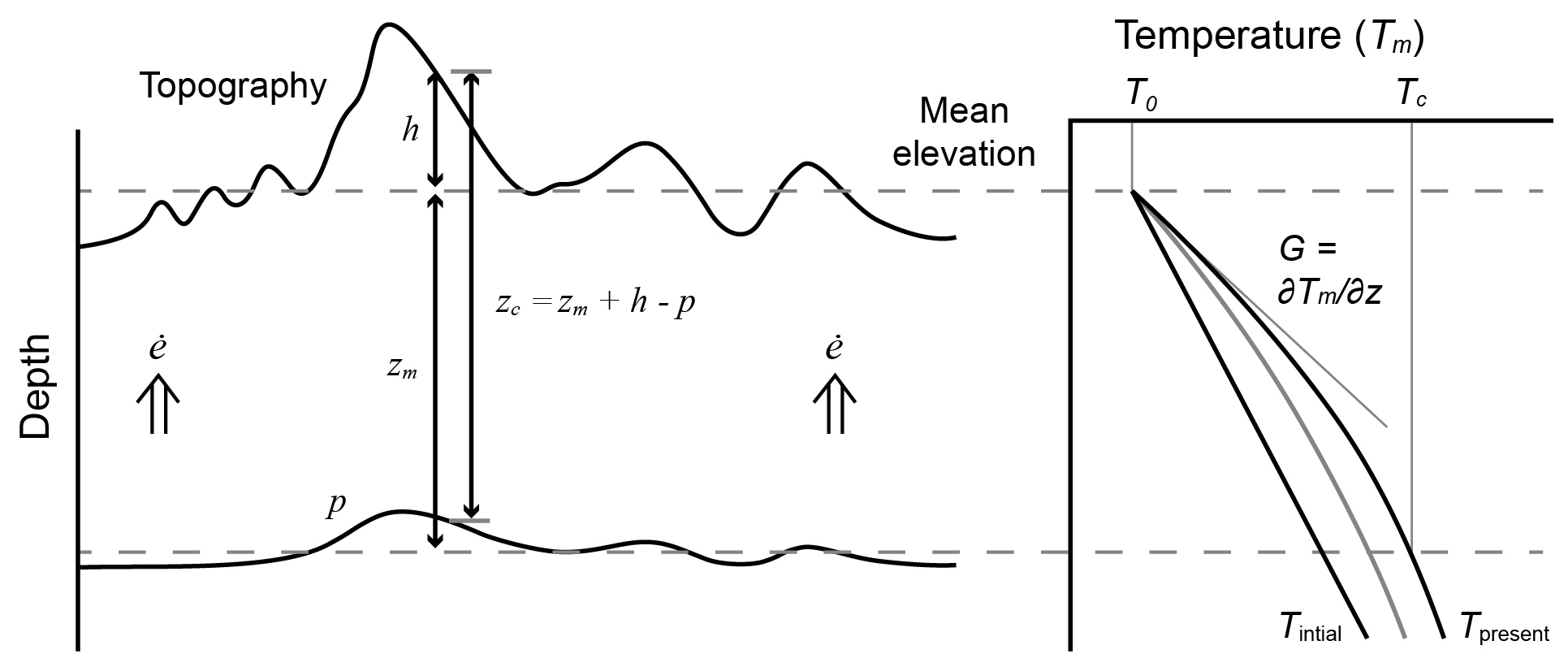
Figure 1 Schematics showing the relationship among closure depth (z_c), topography and its perturbation (p). The parameter h denotes the difference between the sample and the mean elevation, and z_m denotes the depth of the closure temperature (T_c, the lower dashed line) derived from the mean elevation (upper dashed line) and initial temperature field (T_initial) and exhumation history ($\dot{e}$).

The closure temperature (T_c) of a thermochronometer is a function of cooling rate ($\dot{T}$) at the closure time and kinetic parameters of helium and argon diffusion and fission-track annealing in mineral phases (Dodson, 1973):

$$\begin{array}{}\text{(8)}& \dot{T}={\displaystyle \frac{\mathrm{\Omega }R{T}_{\mathrm{c}}^{\mathrm{2}}}{E_{\mathrm{a}}}}\exp \left({\displaystyle \frac{-E_{\mathrm{a}}}{R{T}_{\mathrm{c}}}}\right),\end{array}$$

where Ω and E_a are the diffusion frequency factor normalized by the mineral size and geometry and activation energy, respectively. Parameter R is the gas law constant. See reviews by Reiners and Brandon (2006) for the Ω and E_a parameter values for different thermochronometers.

The cooling rate ($\dot{T}$) can be computed from the derivative of transient geotherms, T_m(t,z) that can be computed using Eq. (7) (Fox et al., 2014):

$$\begin{array}{}\text{(9)}& \dot{T}={\displaystyle \frac{\partial T_{\mathrm{m}}}{\partial t}}+\dot{e}{\displaystyle \frac{\partial T_{\mathrm{m}}}{\partial z}},\end{array}$$

where $\dot{e}$ is unknown exhumation that can be computed through the Eq. (1).

Combining the Eqs. (7)–(9), the closure depth of a thermochronological system (z_c,m) can be numerically computed. This depth also needs a topographic correction because of the topographic perturbation, p, on the isotherms (Braun, 2002; Ehlers and Farley, 2003; Fox et al., 2014; Glotzbach et al., 2015). Such a perturbation can be determined by the following equation (Mancktelow and Grasemann, 1997; Fox et al., 2014):

$$\begin{array}{}\text{(10)}& \begin{array}{rl}p\left(\mathit{\lambda }\right)& =\left({\displaystyle \frac{{\mathit{\gamma }}_{\mathrm{0}}-{\mathit{\gamma }}_{\mathrm{a}}}{{\mathit{\gamma }}_{z_{\mathrm{m}}}}}\right)\\ & \times \exp \left(-z_{\mathrm{m}}({\displaystyle \frac{\dot{e}}{\mathrm{2}\mathit{\kappa }}}+\sqrt{{\left({\displaystyle \frac{\dot{e}}{\mathrm{2}\mathit{\kappa }}}\right)}^{\mathrm{2}}+(\mathrm{2}\mathit{\pi }\mathit{\kappa }{)}^{\mathrm{2}}}\right)h\left(\mathit{\lambda }\right),\end{array}\end{array}$$

where γ_a is the atmospheric lapse rate and γ₀ and ${\mathit{\gamma }}_{z_{\mathrm{m}}}$ are the thermal gradients at the model surface and at the depth z_m. The h(λ) is a cosine function expression of the model surface topography, which can be determined using the discrete fast Fourier transform at the frequency domain. Here we use the SRTM30 data for computing the topography of regions of interest.

Finally, the closure depth of the z_c is corrected by the topographic perturbation (e.g., Brandon et al., 1998):

$$\begin{array}{}\text{(11)}& (z_{\mathrm{c}}{)}_i=(z_{\text{c,m}}{)}_i-p_i+h_i,\end{array}$$

where z_c,m is the closure depth calculated using the 1D geothermal model, p and h are the topographic perturbation and elevation difference with respect to the mean elevation at the sample site (Fig. 1), and the i denotes the ith age.

As shown by the Eqs. (7), (8) and (9), the closure depth is a nonlinear function of rock cooling and exhumation. Therefore, the problem of interest is nonlinear, which can be addressed by iterative numerical modeling methods. In this work, the solution of exhumation is approximated by coupling and iterating the linear inversion and closure depth modeling. As shown in Tarantola (2005) and Fox et al. (2014), the algorithm converges in a few iterations and produces stable outputs.

4 Model evaluation

Quantitative model assessment relies on a misfit value, i.e., the difference between observed and predicted ages weighted by the observed analytical uncertainty:

$$\begin{array}{}\text{(12)}& {\mathrm{\Phi }}_{\mathit{\tau }}=\sqrt{{\displaystyle \frac{\mathrm{1}}{N}}{\sum }_{i=\mathrm{1}}^N{\left({\displaystyle \frac{{\mathit{\tau }}_{\text{prd},i}-{\mathit{\tau }}_{\text{obs},i}}{{\mathit{\epsilon }}_i}}\right)}^{\mathrm{2}}},\end{array}$$

where τ_obs,i and τ_prd,i are the observed and predicted ith age calculated from the exhumation history and ε_i is the uncertainty in the observed ith age. Following Fox et al. (2014), both the a priori and a posteriori misfits, Φ_τ,pr and Φ_τ,po, are determined for the models. The difference between these two misfit values provides a measure of the model improvements. A smaller posteriori misfit value indicates an improved model result and vice versa.

To evaluate the geothermal parameters, we also determined the misfit value of the predicted to the observed modern geothermal gradient value using the following equation:

$$\begin{array}{}\text{(13)}& {\mathrm{\Phi }}_{\mathit{\gamma }}=\sqrt{{\left({\displaystyle \frac{{\mathit{\gamma }}_{\text{prd}}-{\mathit{\gamma }}_{\text{obs}}}{{\mathit{\epsilon }}_{\mathit{\gamma }}}}\right)}^{\mathrm{2}}},\end{array}$$

where γ_prd and γ_obs are the predicted and observed geothermal gradients and ε_γ is the uncertainty in the observed value. Because the depth–temperature curves are slightly nonlinear, the predicted geothermal gradient (γ_prd) is calculated as a mean value for the upper 1 km of the model. Similar to the assessment of age data, we also determined the a priori and a posteriori misfits, Φ_γ,pr and Φ_γ,po values for assessing the geothermal parameters.

5 The reference inverse model

Following Willett and Brandon (2013) and Fox et al. (2014), here we use the published AFT data acquired from Denali Massif (Fitzgerald et al., 1995) for method demonstration (Fig. 2a). A break in slope is shown by the AER at ∼7–6 Ma, indicating a coeval change in slope, i.e., the apparent exhumation rate (Fitzgerald et al., 1995), increasing from 0.17 ± 0.04 to 1.2 ± 0.6 km Myr⁻¹ (Fig. 2b). AER regression of young dates from the lower part of the transect (between 4.3–2.0 km) also predicts a closure depth that is the intercept at −3.3 ± 3.4 km (Fig. 2b). However, using the present geothermal gradient (38.9 °C km⁻¹) (Fox et al., 2014), a nominal closure temperature of AFT method (110 °C) (Reiners and Brandon, 2006) and a −12 °C surface temperature (Fox et al., 2014), the closure depth is predicted as ∼3.1 km beneath the mean elevation (∼4 km), which is equivalent to an elevation of ∼0.9 km. This closure depth is significantly higher than the intercept (−3.3 ± 3.4 km). Such a difference indicates the AER slope of the lower part overestimates the exhumation rates since ∼7–6 Ma.

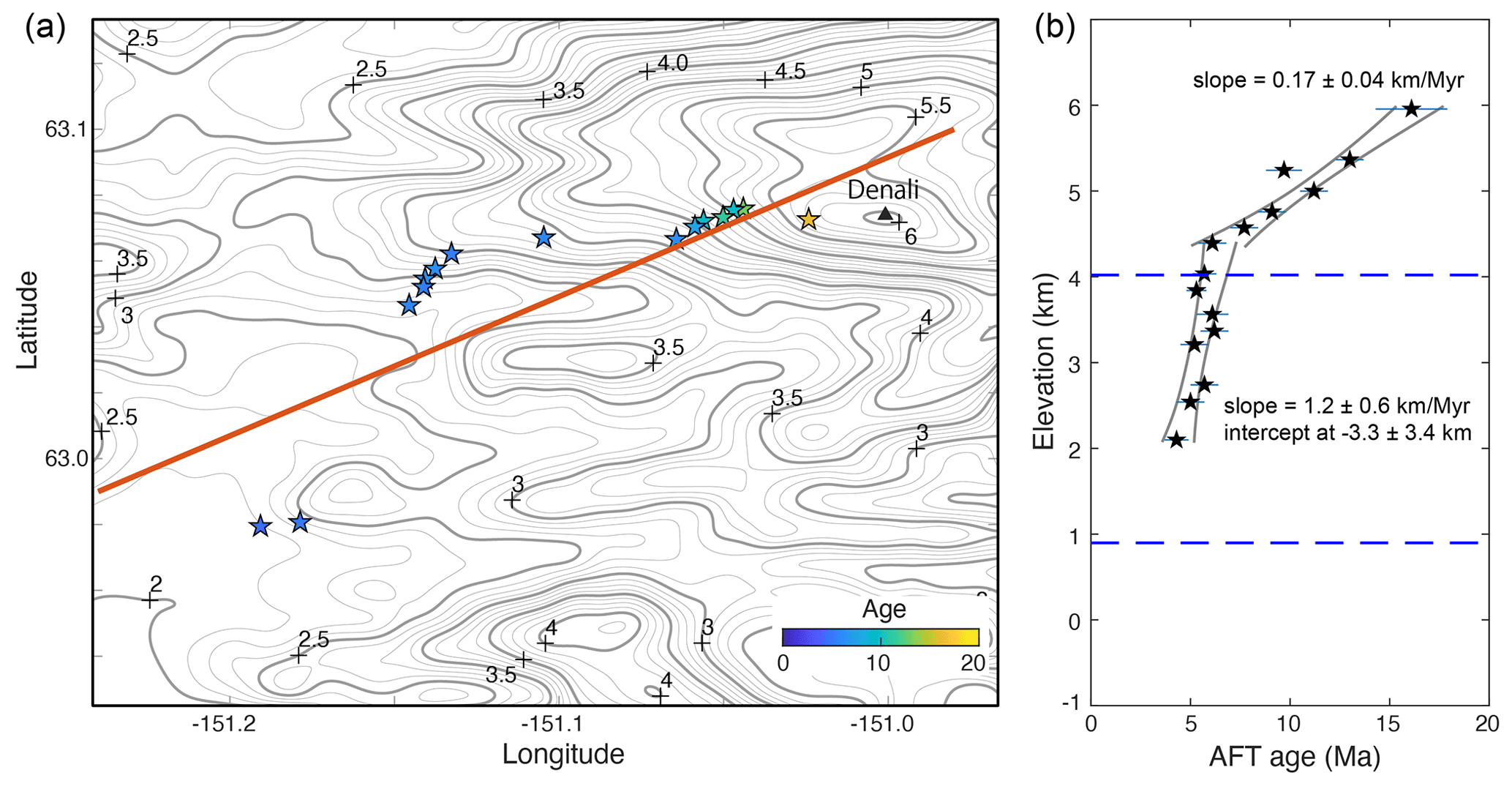
Figure 2 (a) Distribution of AFT age data (pentagons, colored by age values) over the elevation contour map computed using the SRTM30 data of the Denali massif in Alaska. AFT data sourced from Fitzgerald et al. (1995). (b) AER and the slope fitting results using isoplotR (Vermeesch, 2018). AER fitting of ages older than 6.7 Ma yields a slope of 0.17 ± 0.04 km Myr⁻¹, whereas the fitting of ages between 6.5 and 4.3 Ma produces a slope of 1.2 ± 0.6 km Myr⁻¹ and an intercept at −3.3 ± 3.4 km. The upper and lower dashed lines denote the mean elevation (4.02 km) and the depth of the nominal closure temperature (110 °C), calculated using the modern geothermal gradient (38.9 °C km⁻¹) and the surface temperature (−12 °C).

Following the protocol outlined in Fox et al. (2014), the reference inverse model uses the following parameters: a start time at 25 Ma, a time interval (Δt) of 2.5 Myr, a 4020 m mean elevation, a −12 °C surface temperature, an a priori exhumation rate of 0.5 ± 0.15 km Myr⁻¹, a 24 °C km⁻¹ initial geothermal gradient, a 38.9 °C km⁻¹ present geothermal gradient, a model block with a thickness of 80 km and a 30 km² Myr⁻¹ thermal diffusivity.

The exhumation history output of the reference model is shown in Fig. 3. The inversion results reveal an more than 2-fold increase in exhumation rate to a value of ∼0.6 km Myr⁻¹ at 7.5 Ma (Fig. 3b), consistent with the development of the break in slope in the AER. The model also shows a gradual decrease in exhumation rate from a priori exhumation rate (0.5 km Myr⁻¹) to 0.3 km Myr⁻¹ from 25 to 7.5 Ma. The invariant exhumation during the starting stage resulted from the fact that all ages are younger than 17.5 Ma, and thus the data have no resolution for the time span. These results are similar to those of Fox et al. (2014). The a posteriori misfit for the age is 1.88, significantly smaller than that of the a priori model (4.51), suggesting the improvement by the inverse modeling (Fig. 3b). Such a model also provides reasonable fit to the modern temperature field, as shown by the small misfit (0.39) in the geothermal gradient (Fig. 3b).

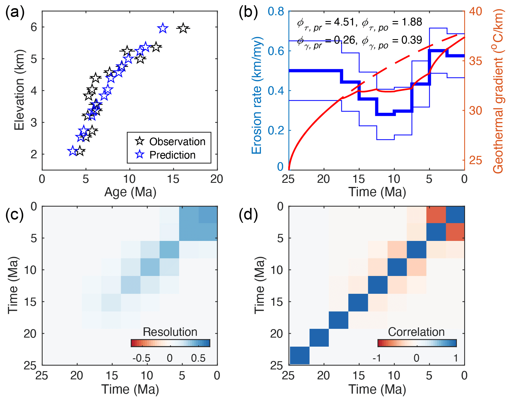
Figure 3 Inputs and outputs of the reference model for the Denali AFT. (a) Comparison between the observed (in black) and predicted (in blue) AER. (b) The a posterior exhumation history generated by the reference model. Thick and thin lines are the mean and 1 standard deviation of the inverted exhumation history. The dashed and solid red lines are the history of the geothermal gradients, predicted by the a priori and a posteriori models, respectively. (c, d) Plots of the resolution and correlation matrix.

The resolution of the inverted exhumation history can be assessed by the resolution matrix R (Eq. 6). Imaging of the matrix shows the model provides no resolution for the time period before 17.5 Ma (Fig. 3c), consistent with the fact that the oldest input age is younger than 16.1 ± 0.9 Ma. For the time span between 15 and 5 Ma, the model resolution is high, as shown by the diagonal elements of the matrix, with the highest resolution at 7.5–5 Ma span, including eight age date points (Fig. 3c). The two most recent phases of exhumation (5–0 Ma) are less resolved, as shown by the nearly equal resolution values for the two phases, i.e., the latest four pixels of the matrix (Fig. 3c). This is because no input ages fall into this time span, when the modeled exhumation results are time-averaged values. The slight decrease in the last stage reflects changes in geothermal gradient.

For assessing the correlation among model parameters, the calculated covariance matrix is scaled by the diagonal covariance matrix (Fox et al., 2014):

$$\begin{array}{}\text{(14)}& {\widehat{C}}_{\mathit{\xi }\mathit{\beta }}={\displaystyle \frac{C_{\mathit{\xi }\mathit{\beta }}}{\sqrt{C_{\mathit{\xi }\mathit{\xi }}}\sqrt{C_{\mathit{\beta }\mathit{\beta }}}}}.\end{array}$$

The correlation matrix for the reference model is shown in Fig. 3d. The diagonal correlation values are 1 and off-diagonal ones are dominantly negative, indicating anti-correlated uncertainties (Fig. 3d), which suggests exhumation parameters were not resolved independently by the modeling. In fact, it is expected to have the anti-correlation because, given two steps of rock exhumation, decreasing the exhumation during one step would increase that of the other step.

6 Dependence on model parameters and proposed solutions

Here we use the Denali data set for demonstrating the influences of (i) the initial geothermal parameters, (ii) the a priori mean and (iii) variance values of the exhumation rates, and (iv) the time interval length on the inverted exhumation history. Also discussed in this section are the solutions for optimizing the model setup for these parameters.

6.1 Dependence on initial thermal model

Different initial model geothermal parameters would lead isotherms to shift either downward to greater depths or upwards to the Earth surface and either compression or expansion among isotherms. Therefore, the initial thermal models have systematic influence on the closure depths and consequently the a posteriori exhumation.

This is demonstrated by modeling experiments presented in Fig. 4. Using a relatively low initial geothermal gradient produces relatively high a posteriori exhumation rates (comparing the models shown in Fig. 4a–f) and vice versa. Such an influence is significant even for the time and elevation intervals with multiple age constraints (10–5.0 Ma). For example, using relatively low geothermal gradients of <22 °C km⁻¹ would yield significantly higher average exhumation rates of >0.75 km Myr⁻¹ for the last two stages (<5 Ma) (Fig. 4a–c) than those (<0.6 km Myr⁻¹) using higher initial geothermal gradients of ≥26 °C km⁻¹ (Fig. 4d–f). Further, it is also shown that models using higher and lower prior geothermal gradients of <20 °C km⁻¹ (Fig. 4a and b) and >30 °C km⁻¹ (Fig. 4e and f) yield worse misfits (${\mathrm{\Phi }}_{\mathit{\gamma },\text{po}}>\mathrm{1}$) for the observed present-day geothermal gradient than those (${\mathrm{\Phi }}_{\mathit{\gamma },\text{po}}<\mathrm{1}$) using medium initial gradients (22–26 °C km⁻¹) (Figs. 3, 4c and d).

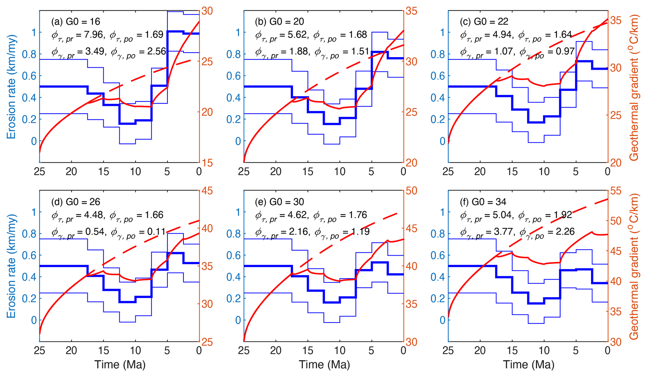
Figure 4 Histories of exhumation and geothermal gradients predicted by models using different initial geothermal gradients between 18 and 34 °C km⁻¹. The thick and thin blue lines are the mean and 1 standard deviation of the inverted exhumation history. The dashed and solid red lines are the history of the geothermal gradients predicted by the a priori and a posteriori models, respectively. Except for the initial geothermal gradient, all other parameters are the same as the reference model. Compared to the reference model, which used an initial geothermal gradient of 24 °C km⁻¹ (Fig. 3), models using a lower initial geothermal gradient yield relatively high exhumation rates (a–c), whereas those using a higher gradient produce lower exhumation rates (d–f).

These results highlight the importance of taking geothermal parameters into account in inverting the exhumation history and model evaluation. We proposed running a set of models using different a priori geothermal parameters, especially the initial geothermal gradient, to search for the proper initial geothermal setup that provides reasonable fits to both the ages and the modern geothermal gradient (see Sect. 7 for details).

6.2 Dependence on the a priori exhumation rate

Both the mean and variance of the a priori exhumation rate have important influences on the model solution for the maximum likelihood estimation method. Our modeling experiments show that the mean value of the a priori exhumation has systematic influences on the inverted exhumation. Similar to the reference model, exhumation of the preceding three stages (25–17.5 Ma) without age constraints is the same as the a priori input. For the following stages, a relatively high mean value of the a priori exhumation results in relatively low a posteriori exhumation rates (comparing different models presented in Fig. 5). For example, models using the mean a priori exhumation of ≤0.4 km Myr⁻¹ yields an a posteriori exhumation of 0.5–0.9 km Myr⁻¹ for the stages <7.5 Ma (Fig. 5a–c), whereas those using a higher a priori value (≥0.6 km Myr⁻¹) result in an a posteriori exhumation of 0.45–0.6 km Myr⁻¹ for the same stages (Fig. 5d–f). This is because a relatively high a priori value, which would be used for calculating thermal models, would lead to a quicker increase in geothermal gradient and thus relatively shallow closure depths and relatively low exhumation rates.

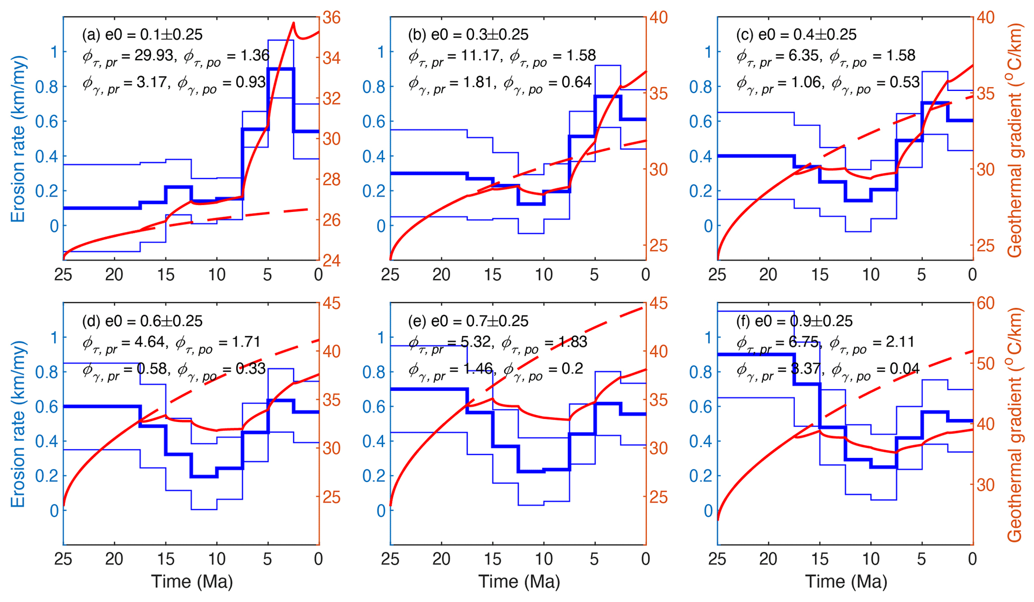
Figure 5 Histories of exhumation and geothermal gradients predicted by models using different a priori mean values of the exhumation rates ranging from 0.1 to 0.9 km Myr⁻¹. Other parameters are the same as the reference model. For an explanation of the plotted lines, see Fig. 4. Compared to the reference model, which used a priori mean exhumation of 0.5 km Myr⁻¹ (Fig. 3), models using a lower a priori exhumation yield relatively high exhumation rates for the last three stages (7.5–0 Ma) (a–c), whereas those using a higher a priori exhumation produce lower exhumation rates for the last three stages (d–f).

The variance of the a priori exhumation rate has an important influence on both the exhumation rates and the posterior variance. Models with lower a priori variances yield fewer variations in the a posteriori exhumation history and vice versa (comparing models in Fig. 6). Further, models using the input variance of the a priori exhumation of 0.2–0.3 km Myr⁻¹ (40 %–60 % of the mean value), the variation in the inverted exhumation history becomes stable (Figs. 3, 6c and d). Given the uncertainty in the input age data, which is often 10 %–20 % at two sigma levels, larger variance of the inverted exhumation would be unreasonable (Fig. 6e and f), especially when multiple age data points are available at different elevations.

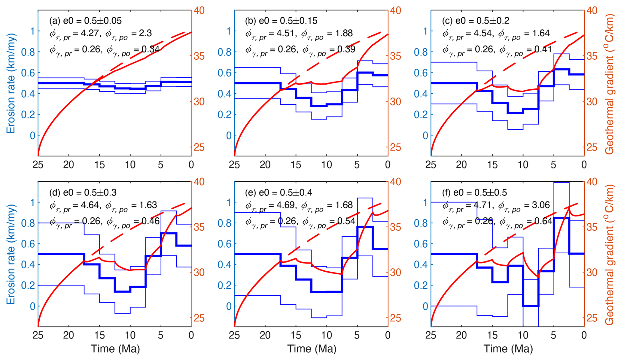
Figure 6 Histories of exhumation and geothermal gradients predicted by models using different a priori variance values (between 0.05 and 0.5 km Myr⁻¹) of the exhumation rates (0.5 km Myr⁻¹). Other parameters are the same as the reference model. For an explanation of the plotted lines, see Fig. 4. Compared to the reference model, which used a priori variance of the exhumation (0.25 km Myr⁻¹) (Fig. 3), models using a lower a priori variance yield limited variations and uncertainties in exhumation (a–c), whereas those using a higher a priori variance produce larger variations and uncertainties (d–f).

We proposed running a set of models using different a priori mean values of erosion rates to search for the one that provides appropriate fits to both the ages and the modern geothermal gradient. As to the a priori variance, we propose using a value 30 %–70 % of the a priori erosion rate. Future applications of the method may need to test a set of the variance inputs so as to get a stable exhumation output. Larger a priori variance would lead to larger uncertainties for the exhumation rates, which is unreasonable and not meaningful for geological studies.

6.3 Dependence on time interval length

Constraining the onset time of major changes in exhumation rates is one of the important tasks for inverting the exhumation history from thermochronologic data. Using a large time interval length cannot accurately capture the potential transition time of exhumation rates. As shown in Fig. 7b–d, models using time lengths of ≤3.5 Myr show an abrupt increase in exhumation at 7–6 Ma, consistent with that shown in AER plot. However, the models using a large time interval length (≥4.5 Ma) overestimate the onset time of the enhanced exhumation (Fig. 7e and f). Further, a relatively short time length would smooth temporal changes in exhumation rates, leading to an underestimating of the variations. For example, as shown in the Fig. 7a, the model using a relatively short time length (0.5 Ma) yields an exhumation variation between 0.35–0.60 km Myr⁻¹, significantly lower than those using relatively larger time interval lengths (Fig. 7b–f). In addition, a shorter time length also significantly increases the computational time and resources, especially when processing a large number of vertical transects.

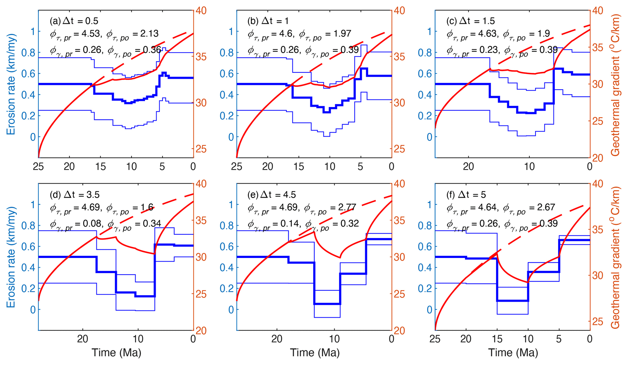
Figure 7 Histories of exhumation and geothermal gradients predicted by models using different time interval lengths. Other parameters are the same as the reference model. For an explanation of the plotted lines, see Fig. 4. Compared to the reference model, which used a time interval length of 2.5 Myr (Fig. 3), models using smaller time interval lengths yield lower variations in exhumation (a–c) than those using larger time interval lengths (d–f).

Given the interests in major exhumation changes, we propose that the time interval length (Δt) should be optimized for constraining the transitional time and the associated exhumation changes. Therefore, the time interval length should be set as the absolute uncertainty at two sigma levels at the break point (τ_b) (Eq. 15). If the break point is unclear in AER, we suggest using the absolute uncertainty at two and three sigma levels at the median age value ($\stackrel{\mathrm{̃}}{\mathit{\tau }}$) (Eq. 15) to focus on the time intervals where ages cluster.

$$\begin{array}{}\text{(15)}& \mathrm{\Delta }\mathit{\tau }=\left\{\begin{array}{ll}\mathit{\delta }{\mathit{\tau }}_{\mathrm{b}},& \text{if a break in slope exists}\\ \mathit{\delta }\stackrel{\mathrm{̃}}{\mathit{\tau }},& \text{if no clear break in AER}\end{array}\right.,\end{array}$$

where δ is the relative age uncertainty at two sigma levels, varying between 10 %–20 % among different studies. Following this method, the Denali case should use a time length of ∼1.5 Ma (7 Ma × 20 %), slightly lower than that used in the reference model (Fig. 3).

7 A new modeling guideline

Following the modeling protocol outlined above, a stepwise modeling guideline is developed for addressing the model dependencies on the initial geothermal parameter, the a priori exhumation rates and time interval length. As illustrated in the Fig. 8, the approach includes the following three steps.

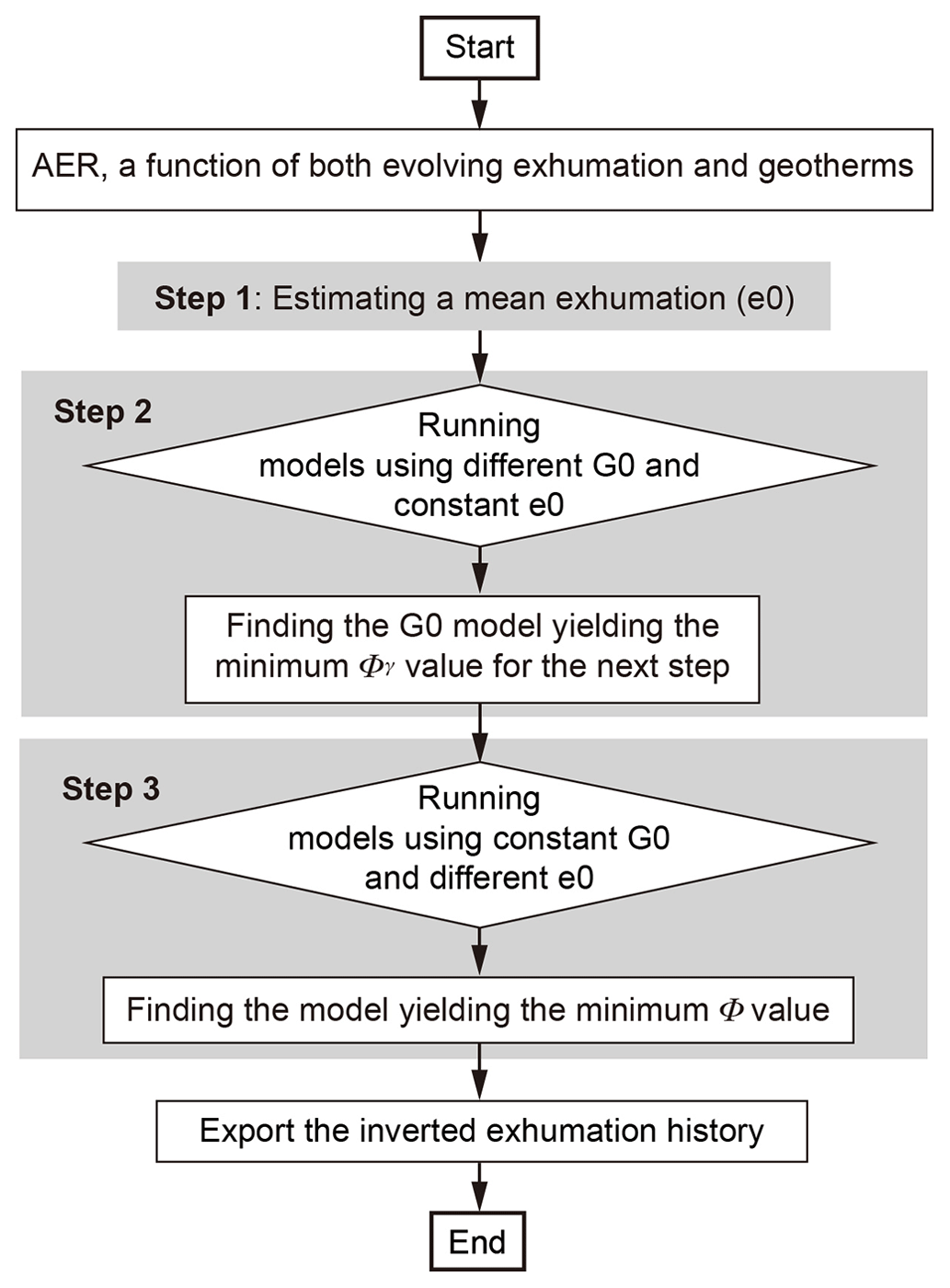
Figure 8 Flowchart of a stepwise modeling method, which includes three main steps. The first step estimates a mean exhumation rate (e0) using the nominal closure temperatures, modern geothermal gradient and sample ages. The mean rate is used in the second step, which runs a set of models using different initial geothermal gradients for optimizing the initial geothermal model. The third step runs a set of models using different a priori exhumation rates, which is generated around the mean rate, and the optimized initial geothermal model by the second step to find the best model that yields the minimum misfit to both age data and modern geothermal gradient.

• i.

  Estimating a time-averaged erosion rate. Dividing each nominal closure depth, which can be estimated from the nominal closure temperatures and the modern geothermal gradient, by the corresponding age results in a time-averaged erosion rate. Following this, a mean value can be determined by averaging the rates. Such a mean value and assumed variance (30 %–50 % in this work) will be used as the a priori erosion rate.

• ii.

  Optimizing the fit to the modern geothermal gradient. This step runs a set of inversion models (20 in this work) using different geothermal gradients, ranging from 50 % to 120 % of the modern value, together with the a priori erosion rate estimated in the first step, for determining the initial geothermal gradient that yields the maximum fit to the modern value, i.e., the minimum Φ_γ (Eq. 13).

• iii.

  Optimizing the fit to both the age data and the geothermal gradient. Given the model dependence on the geothermal parameters (see Sect. 6.1), a comprehensive evaluation of the models should assess not only the age misfit (Φ_τ) but also that of the geothermal gradient (Φ_γ). In the third step, a set of inversion models (20 in this work) are run using different a priori erosion rates, changing from 10 % to 200 % of the mean value estimated in the first step, together with the estimated geothermal gradient by the second step, to search for the model that provides the best fit to both the age data and the modern geothermal gradient. This study uses the following compound misfit function to evaluate the models:

  $$\begin{array}{}\text{(16)}& \mathrm{\Phi }={\mathrm{\Phi }}_{\mathit{\tau }}+{\mathrm{\Phi }}_{\mathit{\gamma }}/\sqrt{N},\end{array}$$

  where Φ_τ and Φ_γ are misfit values for the age and geothermal gradient calculated using the Eqs. (12) and (13) and N is the number of age inputs. Dividing Φ_γ by the square root of N in this equation, as also done for calculating the Φ_τ (Eq. 12), means that the modern geothermal gradient is given the same weight as an age input for evaluating the model.

8 Synthetic models for testing the new modeling guideline

We firstly test our stepwise inversion scheme by using synthetic datasets generated by thermo-kinematic models modified from Braun et al. (2012) (their Fig. 9). The synthetic age dataset is produced by Pecube using the following parameters: a steady-state topography with a 20 km wavelength and a 2 km relief, a model block thickness of 30 km with a basal temperature of 600 °C, a thermal diffusivity of 25 km² Myr⁻¹, a sea level temperature of 10 °C, and a lapse rate of 5 °C km⁻¹. Worth noting is that these parameters are the same as Braun et al. (2012). For model details, see Braun et al. (2012). For the model setup, see Fig. S1 in the Supplement.

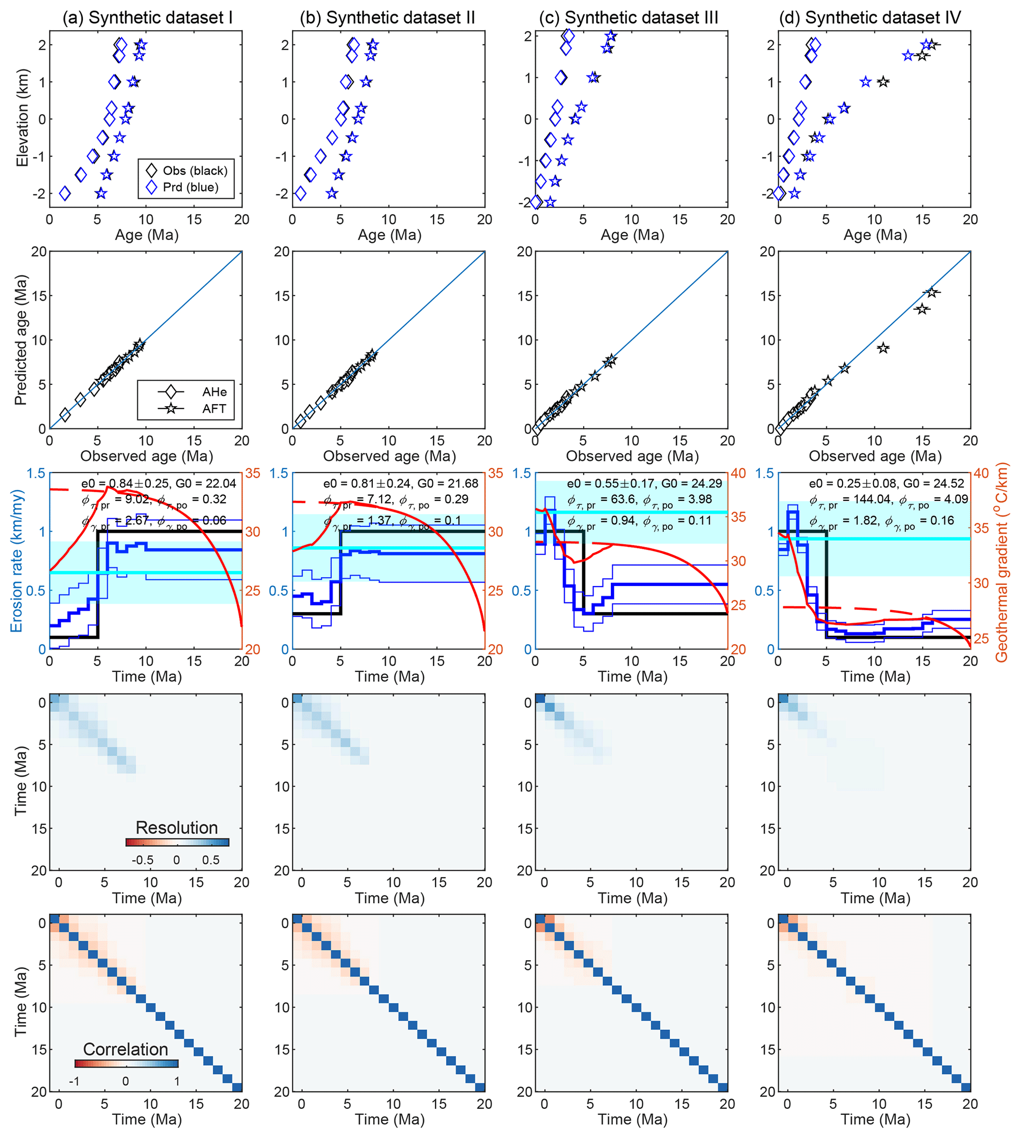
Figure 9 The best-fit model for the synthetic datasets I (a), II (b), III (c) and IV (d) using the modeling method shown in Fig. 8. The top row shows comparisons between the observed (in black) and predicted (in blue) AER. The second row shows plots of observed and modeled ages. The third row shows histories of exhumation and geothermal gradients. The black line marks the “true” exhumation history used for simulating the age dataset, whereas the thick and thin blue lines are the mean and a single standard deviation of the inverted exhumation, respectively. The dashed and solid red lines are the history of the geothermal gradients predicted by the a priori and a posteriori models, respectively, whereas the cyan line and polygon denote the modern geothermal gradient. The fourth and bottom rows show plots of the resolution and correlation matrix, respectively.

Synthetic AFT and AHe ages (Table S1 in the Supplement) were calculated for both surface and borehole samples for four different exhumation histories. The synthetic models I and II are characterized by a sudden decrease in exhumation rate from 1 to 0.1 km Myr⁻¹ (model I, the same as the that shown in Fig. 9 of Braun et al., 2012) and 0.3 km Myr⁻¹ (model II) at 5 Ma, respectively. Models III and IV include a sudden increase in exhumation rate from 0.3 km Myr⁻¹ (model III) and 0.1 km Myr⁻¹ (model IV) to 1 km Myr⁻¹ at 5 Ma. All models start from 40 Ma. Except for the synthetic age data (plotted in the first row of Fig. 9), these four models generate modern geothermal gradients of 26.5, 28.6, 35.5 and 34 °C km⁻¹ for the uppermost 2 km crust, respectively.

The inversion of rock exhumation history used a start time of 20 Ma and a time interval length of 1.0 Myr for all synthetic datasets, which were assigned with a 6 % uncertainty. As shown by the modeling output visualized in Fig. 9a, our inversion of the rock exhumation from the synthetic dataset I finds an optimal initial geothermal gradient of 22 °C km⁻¹ and a priori rate of 0.85 ± 0.25 km Myr⁻¹ and yields a decrease in exhumation rates from ∼0.9 km Myr⁻¹ (before 6 Ma) to 0.3–0.1 km Myr⁻¹ (4–0 Ma) via a gradual decrease during 6–4 Ma. The data have no resolution for the exhumation history before 10 Ma. Compared to the synthetic model (abrupt decrease from 1 to 0.1 km Myr⁻¹ at 5 Ma), the rates before 5 Ma are underestimated by 0.1 km Myr⁻¹, whereas the values after 5 Ma are overestimated by 0.1–0.3 km Myr⁻¹.

The inversion for synthetic dataset II results in an optimal initial geothermal gradient of 21.7 °C km⁻¹, an a priori rate of 0.81 ± 0.24 km Myr⁻¹ and an increase in exhumation rates from ∼0.85 (before 5 Ma) km Myr⁻¹ to 0.4–0.5 km Myr⁻¹ (4–0 Ma) via a gradual decrease during 5–4 Ma (Fig. 9b). Compared to the synthetic model (abrupt decrease from 1 to 0.3 km Myr⁻¹ at 5 Ma), the rates before 5 Ma are underestimated, whereas the values before 5 Ma are overestimated by ∼0.1–0.2 km Myr⁻¹.

The inversion for synthetic dataset III yields an optimal initial geothermal gradient of 24.3 °C km⁻¹, an a priori rate of 0.55 ± 0.17 km Myr⁻¹ and a decrease in exhumation rates from ∼0.45–0.3 km Myr⁻¹ (before 5 Ma) to 1.0 km Myr⁻¹ (3–0 Ma) via a gradual increase during 5–3 Ma (Fig. 9c). Compared to the synthetic model (abrupt decrease from 0.3 to 1.0 km Myr⁻¹ at 5 Ma), the rates during 5–3 Ma are underestimated, whereas the rates before 5 Ma are overestimated by 0–0.15 km Myr⁻¹.

The inversion for the synthetic dataset IV produces an optimal initial geothermal gradient of 24.5 °C km⁻¹, an a priori rate of 0.25 ± 0.08 km Myr⁻¹ and an increase in exhumation rates from ∼0.1–0.2 km Myr⁻¹ (before 5 Ma) to 1.0 km Myr⁻¹ (3–0 Ma) via a gradual decrease during 5–3 Ma (Fig. 9d). Compared to the synthetic model (abrupt decrease from 1 to 0.3 km Myr⁻¹ at 5 Ma), the rates before 5 Ma are slightly overestimated, whereas the values during 5–3 Ma are underestimated.

To summarize, the inverted rock exhumation histories for the four synthetic datasets match the whole picture of the synthetic “truth”, but the variations in exhumation are underestimated, and the sharp changes at 5 Ma are smoothed. It is worth noting that inversions using only surface samples produce similar inversion results (Fig. S2 in the Supplement).

9 Natural examples for testing the new modeling guideline

Below we use three examples to demonstrate our new method. The Denali data are used again for demonstrating the efficiency of our method in finding the proper initial geothermal gradient and the a priori exhumation rate. Following this, we further test our method using the Himalayan Dhanladar range and KTB borehole (the Continental Deep Drilling Project in Germany) thermochronologic data for representing regions of fast and slow erosion, respectively.

9.1 The Denali transect

Using the stepwise inversion modeling guideline, the Denali transect yields an exhumation history generally similar to that of the reference model (Fig. 10a). Differences in the a priori parameters include that the new inversion finds and uses an initial geothermal gradient of 25.2 °C km⁻¹ (slightly higher than that of the reference model), an a priori erosion rate of 0.46 ± 0.23 km Myr⁻¹ (slightly lower than that of the reference model) and a time interval length of 1.5 Ma. The combination of these a priori parameters results in a major increase in erosion rate to 0.55–0.6 km Myr⁻¹ at 6 Ma, which is 1.5 Myr later than that of the reference model (7.5 Ma). The subtle differences from the reference model mainly result from the time interval length used in these models. Comparing the misfit values, the new model produces slightly better fits than the reference model, with the a posteriori misfit values of 1.81 and 0.11 for the observed age and geothermal data.

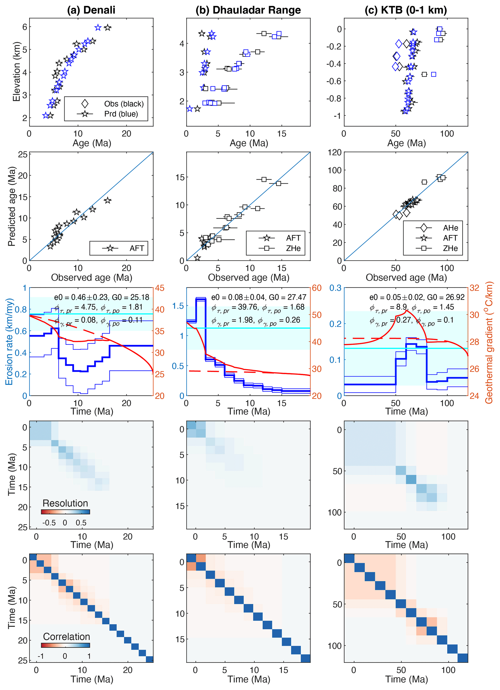
Figure 10 The best-fit model for the Denali (a), Dhanladar range (b) and upper KTB (c) transects using the modeling method shown in Fig. 8. See Fig. 8 for panel interpretations.

9.2 Himalayan Dharladar range transect

AFT and ZHe data from the Dharladar range in the northwestern Himalayas, reported in the publications by Deeken et al. (2011) and Thiede et al. (2017), are used as an example for regions of young cooling ages and fast exhumation. The samples were collected in an elevation range between 1.5 and 4.5 km, covering a topographic relief of 3 km within a spatial distance of ∼15 km on the hanging wall of the main central thrust of the Himalayan fold and thrust belt (Deeken et al., 2011; Thiede et al., 2017). AER slope regression of ZHe and AFT ages performed in Deeken et al. (2011) produced apparent erosion rates of ∼2.8 and ∼0.2 km Myr⁻¹ for the time intervals 6.4–14.5 and 1.7–3.7 Ma, respectively, implying a potential increase in erosion rates at ∼3.7–6.4 Ma. Using geothermal gradients of 25–45 °C km⁻¹, time-averaged erosion rates were estimated as 0.8–2.0 km Myr⁻¹ since 3.7 Ma (Deeken et al., 2011).

The modeling of the Dharladar range data uses a modern geothermal gradient constraint of 45 ± 8 °C km⁻¹ (Deeken et al., 2011). The relatively large uncertainty is assigned for the geothermal gradient because of the absence of direct geothermal measurements in the study area. Our exhumation inversion for the AER data using the stepwise modeling guideline yields relatively slow rates of 0.1–0.6 km Myr⁻¹ and fast rates of 1.2–1.6 km Myr⁻¹ before and after ∼3 Ma, respectively (Fig. 10b). The abrupt increase in exhumation rates at ∼3 Ma is generally consistent with the estimates from the slope regression results of Deeken et al. (2011). However, the inverted exhumation rates since 3 Ma are significantly lower than the estimation from the AER slope (∼2.8 km Myr⁻¹), which is likely due to the overestimation of exhumation of the AER slope due to topographic perturbation of isotherms. Such a perturbation is a function of exhumation rates: the higher the exhumation, the larger the perturbation (Glotzbach et al., 2015). The modeling yields a history of the geothermal gradient that gradually increases to a modern value of ∼46 °C km⁻¹, close to the input value (45 ± 8 °C km⁻¹).

9.3 KTB borehole

The KTB borehole yields a large amount of thermochronologic and geochronologic age data (Warnock and Zeitler, 1998; Stockli and Farley, 2004). Previous studies suggest the borehole is truncated by multiple faults, which offset the age–depth relationship (Wagner et al., 1997). Here we use the data at depths shallower than 1 km, where data are abundant and have linear relationship with depths.

The KTB apatite, zircon and titanite $\left(\mathrm{U}\text{-}\mathrm{Th}\right)/\mathrm{He}$ (AHe, ZHe and THe) and AFT age data vary greatly between 85–50 Ma. These clustered ages have been interpreted as indicating a late Cretaceous phase of exhumation, followed by slow exhumation (Wagner et al., 1997; Stockli and Farley, 2004), as also shown by previous thermal history reconstructions based on K feldspar ${}^{\mathrm{40}}\mathrm{Ar}{/}^{\mathrm{39}}\mathrm{Ar}$ data (Warnock and Zeitler, 1998).

Our modeling, using the AER data and a modern geothermal gradient of 27.5 ± 2.8 °C km⁻¹ (Clauser et al., 1997), shows that elevated exhumation rates (0.1–0.13 km Myr⁻¹) between 80–50 Ma, followed by slower exhumation rates of ∼0.04 km Myr⁻¹ (Fig. 10c), are similar to previous estimates (Wagner et al., 1997; Warnock and Zeitler, 1998; Stockli and Farley, 2004). Associated with changes in exhumation, the geothermal gradient gradually decreases from the peak values at 70–60 Ma to a value of ∼28 °C km⁻¹ at the present day.

10 Conclusion

The a priori information has important effects on the inversion results using the least-squares inversion method. Our study demonstrates the importance of geothermal gradient and the a priori exhumation rate in estimating the exhumation history from the thermochronology data. To take into account the geothermal data for the exhumation history inversion, we outlined a stepwise inversion method that first searches for the appropriate initial geothermal gradient, which is then used in the modeling searching for the a priori exhumation rate. Our modeling guideline produces an exhumation history and a geothermal gradient that provide reasonable fits for both the observed AER and modern geothermal data, as tested by datasets of both synthetic models and natural samples.