Machine learning prediction of the mass and the velocity of controlled single-block rockfalls from the seismic waves they generate

Understanding the dynamics of slope instabilities is critical to mitigate the associated hazards, but their direct observation is often difficult due to their remote locations and their spontaneous nature. Seismology allows us to get unique information on these events, including on their dynamics. However, the link between the properties of these events (mass and kinematics) and the seismic signals generated is still poorly understood. We conducted a controlled rockfall experiment in the Riou Bourdoux torrent (southern French Alps) to try to better decipher those links. We deployed a dense seismic network and inferred the dynamics of the block from the reconstruction of the 3D trajectory from terrestrial and airborne high-resolution stereophotogrammetry. We propose a new approach based on machine learning to predict the mass and the velocity of each block. Our results show that we can predict those quantities with average errors of approximately 10 % for the velocity and 25 % for the mass. These accuracies are as good as or better than those obtained by other approaches, but our approach has the advantage in that it does not require the source to be localised, nor does it require a high-resolution velocity model or a strong assumption on the seismic wave attenuation model. Finally, the machine learning approach allows us to explore more widely the correlations between the features of the seismic signal generated by the rockfalls and their physical properties, and it might eventually lead to better constraints on the physical models in the future.

1 Introduction

Slope instabilities are complex natural phenomena that pose a threat to humans and infrastructures in many regions of the world. Landslides, rockfalls, rock avalanches, and surface collapses generating pit craters are natural disasters that can affect our societies. They also play a major role in the Earth surface dynamics as important erosion processes, whose occurrence might be caused by external factors such as earthquakes, intense precipitation, or the thawing of ice in the joints and fractures of large rocky masses. Understanding the triggering mechanisms and their dynamics and quantifying and documenting their properties and their spatiotemporal occurrences are of paramount importance to mitigate the associated risks but also to understand their contributions to long- and short-term erosion processes. However, because of their spontaneous and destructive nature, gravitational instabilities are difficult to study.

Over the past 2 decades, these processes have been increasingly studied through the use of approaches based on seismology. Seismology makes it possible to augment the source of information conventionally deployed to study mass-wasting processes (e.g., direct testimony, remote sensing, geomorphology, geodetic measurements) by its ability to provide information on event properties, such as the exact time of occurrence (to the second) and the localisation (e.g., Norris, 1994; Deparis et al., 2008; Yamada et al., 2012; Hibert et al., 2014; Dammeier et al., 2011, 2016; Gracchi et al., 2017; Dietze et al., 2017; Allstadt et al., 2018; Yan et al., 2019; Kuehnert et al., 2020b), with the possibility of recording them over vast distances (up to 1000 km for the largest events) (e.g., Kanamori and Given, 1982; Kanamori et al., 1984; Ekström and Stark, 2013; Allstadt, 2013; Hibert et al., 2019). More than providing spatiotemporal information, sometimes in real time, seismology offers the possibility to retrieve the dynamics of an event through the information carried by the seismic signal emitted during the triggering and the propagation of the event. There are very few other observational approaches that allow retrieval of important insights on the dynamics. Hence, finding relationships between seismic signals generated by gravitational instabilities and their properties has been a major focus of recent research in landslide and rockfall seismology.

For catastrophic landslides (volume over 1 ×10⁶ m³), approaches based on the inversion of the long-period (low-frequency, below 0.5 Hz) seismic waves have been proposed. By retrieving the force exerted by the mass displacement on the Earth, those approaches have successfully helped to determine dynamic parameters (velocity, momentum, and acceleration) and properties of these events (e.g., Kawakatsu, 1989; Ekström and Stark, 2013; Allstadt, 2013; Zhao et al., 2012; Iverson et al., 2015; Hibert et al., 2015, 2017a; Moore et al., 2017; Dufresne et al., 2019; Li et al., 2017; Moretti et al., 2020; Chao et al., 2018; Zhang et al., 2019). However, most mass-wasting processes that occur worldwide do not have a volume large enough to generate those long-period waves, thus precluding the use of inversion methods to retrieve their dynamic quantities, yet those mass-wasting processes will generate high-frequency seismic waves (frequency above 1 Hz). Being able to infer physical properties from those high-frequency seismic waves will therefore allow us to characterise most mass-wasting processes, including smaller-volume events, which is critical to have a better understanding of the occurrence and the physics of those phenomena and thus to mitigate the risks they generate.

Recent studies proposed scaling laws between high-frequency seismic signal features and source properties of rockfalls and landslides. These studies are mostly based on laboratory experiments (e.g., Farin et al., 2015, 2016, 2019; Arran et al., 2020), real-scale experiments (e.g., Bottelin et al., 2014; Hibert et al., 2017b; Saló et al., 2018), and documented natural events (e.g., Norris, 1994; Deparis et al., 2008; Dammeier et al., 2011; Hibert et al., 2011; Levy et al., 2015; Hibert et al., 2017a; Le Roy et al., 2019). Among the quantities studied, several correlations between the mass and the velocity of the rockfall and the magnitude, the maximum amplitude at the source, and the seismic energy of the seismic signal have been observed and sometimes quantified. Several scaling laws have been proposed (e.g., Norris, 1994; Deparis et al., 2008; Hibert et al., 2011; Levy et al., 2015; Hibert et al., 2017b; Saló et al., 2018; Le Roy et al., 2019), but they all carry strong uncertainties, caused mainly by the simplicity of the propagation models used (e.g., Le Roy et al., 2019; Kuehnert et al., 2020a), the difference in contexts (soft soil vs. hard rock and the influence of the seismic network geometry), and the physics of the source (free-fall, granular flows, single rockfall, and multiple rockfalls). However, all of those studies demonstrated that there is a link between some seismic signal features (maximum amplitude at the source, seismic energy, and local magnitude) and some source properties (mass, velocity, energies, momentum, force, or acceleration). The difficulty now resides in understanding the fundamental physics that explains those correlations and in increasing the accuracy of the scaling laws proposed. This is deemed important as it opens the perspective to quantify mass-movement dynamics directly from the seismic signals they generate (i.e., without inversion or modelling). This is critical for the development of future methods aimed at their real-time detection and characterisation using high-frequency seismic signals. This can be achieved by improving both the source physical model and the seismic wave propagation model, which remains a strong challenge for high-frequency seismic waves. These improvements require more high-quality observations to calibrate and validate the models. This is what motivated the 2018 Riou Bourdoux controlled rockfall experiment, which followed and improved upon a similar experiment conducted in 2015 (Hibert et al., 2017b).

Thanks to the deployment of a dense seismological network close to the block impacts and an approach allowing an accurate reconstruction of the trajectories (Noël et al., 2022), we tried to complete three objectives: (1) better understanding and modelling the propagation of the seismic waves generated by the block impacts; (2) finding and trying to better constrain the correlations between the kinematic parameters of the impacts of the blocks and the features of their seismic signals, and (3) exploring the use of an innovative approach based on a machine learning algorithm to infer the mass and the velocity of the block at each impact from the seismic signals generated.

2 Material and methods

2.1 Context: the Riou Bourdoux catchment

The Riou Bourdoux is a torrential catchment located in the southern French Alps, approximately 4 km north of the city of Barcelonnette (France). It formed in Callovo–Oxfordian black marl whose high erosion susceptibility resulted in the formation of numerous steep (> 30 °) gullies. The blocks were launched in a gully located on the northern slope of the torrent. The travel path had a length of approximately 200 m and slope angles ranging from 45° on the upper part of the slope to approximately 20° on the terminal debris cone (Fig. 1). The launched elements consisted of hard limestone blocks selected in the torrent and brought to the launch pad with a backhoe.

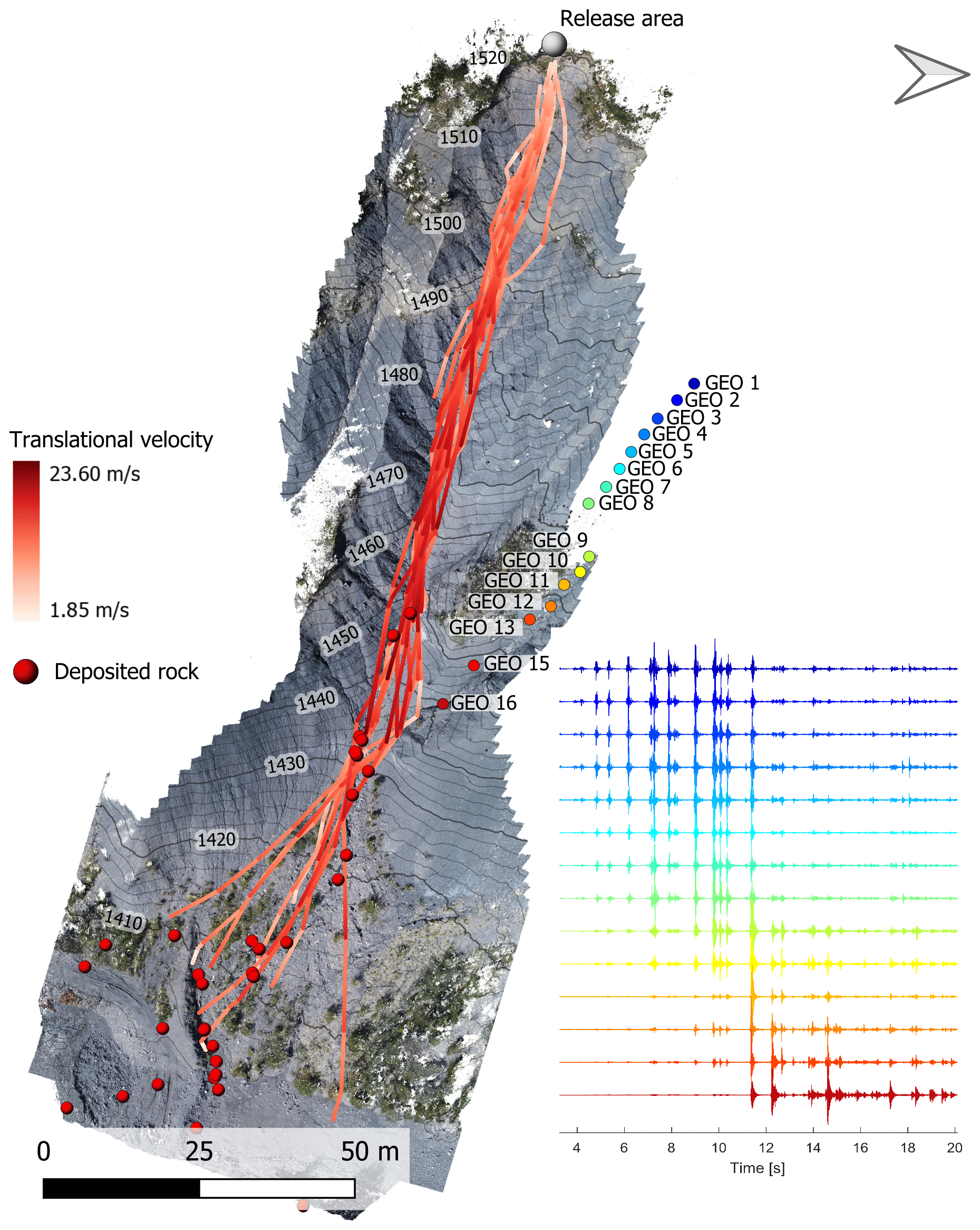
Figure 1 Orthophotography of the Riou Bourdoux gully, with the reconstructed trajectory of all the blocks, and the location of the geophones used in this study indicated by coloured dots. The colour of the trajectory scale represents the absolute translational velocity of the block. The raw seismic signals recorded at each geophone for the first launch are represented on the right in the colour corresponding to the one of the dots, indicating the location of the sensor.

2.2 Block trajectories and properties measurements

Kinematic parameters of each launch were computed from 31 reconstructed rockfall trajectories using the ballistic equations of a free-falling object neglecting the drag from the air (Volkwein et al., 2011; Wyllie, 2014; Loew et al., 2021). The back-calculation method using 3D terrain models and video footage (Noël et al., 2017, 2022) requires accurately measuring the geometric features of each launched block and of the terrain and to track their propagation with high-speed multispectral cameras from different viewing angles.

A total of 31 limestone blocks were individually weighted using a lift and a tension load cell. The density of the rocks was determined in the laboratory from analysis conducted on core samples taken from each block. The block shapes were acquired using mobile handheld terrestrial laser scans (mobile terrestrial laser scanning GeoSLAM ZEB Revo) and from structure-from-motion photogrammetry (SfM) using pictures acquired with a Panasonic GH5 camera and the software Agisoft Metashape Pro v.1.4.4. The laser model served as a reference for adjusting the scale of the photogrammetric model, ensuring it remained undistorted, followed by employing the ICP algorithm to align the photogrammetric model with the laser model after manually excluding non-overlapping areas. Additionally, to determine the final shape and volume of the blocks, a flat base was added to each block to align it with the surrounding terrain, enabling volume calculation through mesh modelling, with mass deduced from homogeneous density assumptions based on measured samples as detailed in Noël et al. (2022). The lidar model has a spatial density of about 50 000 points per m² at the block level. The SfM model was built from 128 photos for each block and has a density of about 5 million points per m² when scaled (average: 4.93 × 10⁶ pts m⁻²; standard deviation: 2.123 × 10⁶ pts m⁻²). Assuming a homogeneous distribution of the mass, the moments of inertia of each block and the main axes of inertia were identified from the 3D models of each block and the density. Their dimensions were measured on the 3D models aligned on their main axes of inertia. The mass of each block ranged from 39 to 468 kg.

A very high-resolution terrain model of the gully (Fig. 1) was acquired using four acquisition methods to ensure proper coverage of occluded faces, detailed texture of the surfaces, and accurate scale and orientation relative to the horizontal. A highly detailed terrain SfM model was generated from georeferenced pictures acquired with a DJI Phantom 4 UAV flying at an average altitude of 25.3 m. We use the software Agisoft Metashape Pro v.1.4.4. The model was built from 167 photos with resolution of 5472 × 3078 pixels and with a selected overlap of at least 9 images. The initial model had 345 922 467 points with a ground resolution of 6.32 mm px⁻¹ and was downscaled to 83 475 710 points spaced by 1 cm. Its scale was then adjusted by less than 1 % using the iterative closest point algorithm to match with a detailed terrain model obtained from four locations (Fig. 1) with a terrestrial laser scanning device (Optech ILRIS-LR) (Noël et al., 2022). The main gully was also scanned with a mobile terrestrial laser scanning while rappelling down to cover every part in detail. Finally, evenly spread targets were painted in the upper and lower part of the gully and were located using a laser theodolite.

The blocks were pushed down manually one by one, separated by about 5 to 10 min. There was no sliding in the early stage of those triggered rockfalls. Their trajectories were manually tracked from up to eight viewpoints: five viewpoints had fixed framing, being installed on tripods (one in the middle part of the travel path and four at the bottom of the gully); two viewpoints were from the sky using two DJI drones, with one flying in hover and one following the motion of the blocks; and the last viewpoint was from a camera panned manually to track the rocks using a long-focus lens and was located at the bottom of the gully. An exhaustive description of the experiment and the approach to reconstructing the trajectories, as well as videos showing the propagation of the blocks and the numerical approach to reconstructing the trajectories, is given in the paper by Noël et al. (2022), companion to the present article.

2.3 Seismic network and data

The seismic network was deployed along the gully. The network comprised 16 three-component geophones (4.5 Hz 3C connected to a DAQlink seismic camera at a sampling rate of 1000 Hz). The exact positions of the sensors were measured by differential GNSS (Fig. 1). In this analysis, we used only the vertical components of the geophones as we observed the best signal-to-noise ratio on this component. Data from geophone numbers 14 and 16 were discarded as the records exhibited high-amplitude noises and spikes probably related to a faulty connection or a bad installation. Before analysis, each record was deconvolved from the instrument response to get the ground velocity. No filtering was applied to the raw data.

2.4 Trajectory and kinematics reconstruction

The impact locations of each block were pointed on the 3D textured detailed terrain model (Fig. 1). The task was eased by using custom-developed software (Noël et al., 2022) in which the terrain can be visualised from the same viewpoints as the corresponding video footage and in which the reconstructed trajectories offset by the radius of each rock are updated in real time following the cursor mouse or manually entered impact coordinates. The position and time of each impact can thus be accurately defined until obtaining visually matching trajectories with those visible in the camera footage. With non-optimal viewing angles or terrain texture with little contrast, screenshots of the terrain model and video footage were aligned with the Handle Transform Tool in the GIMP software using the surrounding elements of texture in order to find the exact location of the impact.

The trajectories were exported with their velocities and vectors normal to the terrain, and the centre of mass of the blocks was extrapolated from the impact position on the ground. All trajectories were further visually inspected in the CloudCompare software. The angular velocities were obtained by averaging the number of block revolutions performed during the period in between each impact. The average axis around which the block rotated was identified to estimate the angular momentum based on the geometric features of each block. We removed from our dataset every impact that resulted in a breaking of the block. We have kept only the impacts for which the block did not undergo major changes according to our visual observations. We cannot exclude a marginal change in the mass of the block due to successive impacts, but this should not have a major impact on our results.

In total, 376 impacts were available from 25 trajectory segments composed of many parabolas. The impacts at the extremities of each segment are missing because of missing incoming/outcoming velocities. Therefore, 326 impacts were reconstructed with their incoming and outgoing translational and angular velocities, kinetic energy changes, and momentum.

2.5 Trajectories and seismic records synchronisation

While the seismological data could be time-stamped by a GNSS, the clocks of the different cameras used during the experiment were not all set to the absolute time. To determine the lag between the two time series (time of impact from the direct observations and seismic records) with a precision below the second, we performed a cross-correlation analysis. The timing of the impacts was transformed into a time series of zeros and ones, with zeros indicating the times with no impact and ones indicating the time of each impact. We then normalised the seismic records by the maximum of the envelope and computed the cross-correlation between the impacts time series and the normalised envelope of the seismic records, with lags ranging from minus 10 to plus 10 s. The lag for which the best normalised correlation was observed was selected. A manual control and final adjustment of the results was performed. After this first step we manually picked the beginning and the end of each seismic signal on each station. We selected only the signals associated with impacts that did not result in the fracturing of the blocks and that were not generated by parts of fragmented blocks. This was verified for each impact on the videos of the launches. We also selected only impacts for which it was possible to pick clearly the beginning and the end of the seismic signal and therefore discarded all intricate and low-amplitude seismic signals. An example of the seismic signals recorded at one station and of the selected impact seismic signals is presented in Fig. 2. This resulted in a dataset of 384 seismic signals of impacts.

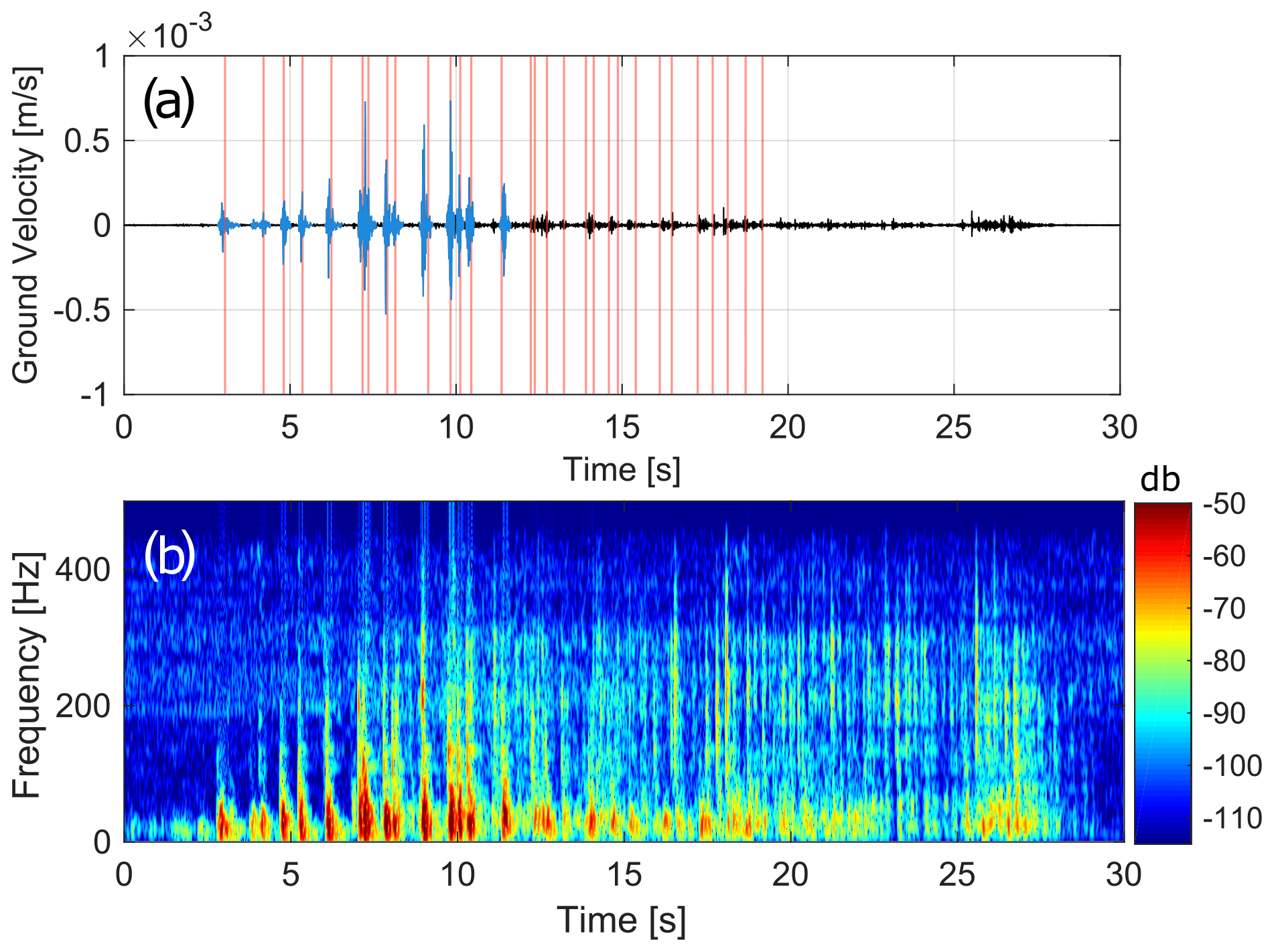
Figure 2 Seismic signal (a) and spectrogram (b) generated by impacts of Block 1 and recorded on Geophone 1. The selected seismic signals used in our analysis are indicated in blue. The impact times derived from the camera-based workflow for this launch are indicated by red lines in panel (a).

2.6 Seismic source parameter computation

There are essentially two properties of high-frequency seismic signals generated by mass movements that have been studied in correlation with the physical parameters of the source dynamics: the maximum amplitude of the seismic signal corrected for propagation effects A₀ and the energy of the seismic signal at the source E_s (e.g., Norris, 1994; Deparis et al., 2008; Dammeier et al., 2011; Schneider et al., 2011; Hibert et al., 2011; Bottelin et al., 2014; Levy et al., 2015; Farin et al., 2015, 2016; Hibert et al., 2017b, a; Saló et al., 2018; Le Roy et al., 2019; Farin et al., 2019; Arran et al., 2020). These two quantities are usually compared to the source velocity and momentum and to its kinetic and potential energies. Both quantities are computed from attenuation parameters that allow us to account for the attenuation of seismic waves caused by the propagation of waves in the earth and which are caused by geometrical spreading and anelastic attenuation. Determining an adequate attenuation model is therefore critical.

Thanks to the reconstruction of the trajectories, in our study we know the exact location of the impact and hence the distances between the source and the receivers; thus we could test several attenuation models and find the one that better explains the observed decay of the amplitudes with the distance. We consider the 3D point-to-point direct distance without taking into account the topography. The best model should be the one that allows the best regression of the maximum amplitude of each impact recorded at each station as a function of the distance of those stations to the location of the impact.

We tested two simple attenuation models, one for surface wave (Eq. 1) and one for body wave (Eq. 2), both proposed by Aki and Chouet (1975), which consider the anelastic attenuation of seismic waves through the use of the attenuation factor β:

$$\begin{array}{}\text{(1)}& {\displaystyle }A\left(r\right)=A_{\mathrm{0}}{\displaystyle \frac{e^{-\mathit{\beta }r}}{\sqrt{r}}},\text{(2)}& {\displaystyle }A\left(r\right)=A_{\mathrm{0}}{\displaystyle \frac{e^{-\mathit{\beta }r}}{r}}.\end{array}$$

The maximum amplitude at the source A₀ and the β factor can be determined directly from the attenuation model for each impact.

An approximation of the seismic energy for body waves can be computed as per Crampin (1965):

$$\begin{array}{}\text{(3)}& E_{\mathrm{s}}=\underset{t_i}{\overset{t_{\mathrm{f}}}{\int }}\mathrm{4}\mathit{\pi }{r}^{\mathrm{2}}\mathit{\rho }c{u}_{\mathrm{env}}(t{)}^{\mathrm{2}}{e}^{\mathit{\beta }r}\mathrm{d}t,\end{array}$$

with

$$\begin{array}{}\text{(4)}& u_{\mathrm{env}}\left(t\right)=\sqrt{u(t{)}^{\mathrm{2}}+\mathrm{Ht}(u\left(t\right){)}^{\mathrm{2}}},\end{array}$$

where Ht is the Hilbert transform of the seismic signal u(t) used to compute the envelope u_env(t), t_i and t_f are the times of the beginning and the end of the seismic signal respectively, ρ is the density of the layer through which the generated surface waves propagate, and c is their phase velocity. The average velocity of body waves in black marl is approximately 450 m s⁻¹ (Hibert et al., 2012; Gance et al., 2012). The density ρ of dry black marl is approximately 1450 kg m⁻³ (Maquaire et al., 2003). For each impact we computed the seismic energy at each station and kept the mean over all stations.

2.7 Machine learning: using random forests as a regression tool

Random forest (Breiman, 2001) (RF) is a machine learning algorithm based on the computation of a large number of decision trees. Decision trees are top-down structures consisting of nodes and branches. At each node a statistical test is performed on the value of one feature of the input data. The outcome of this test tells which branch to use to get the next node. The final nodes of the tree give the decision of the tree. The randomness comes from the use of a random subset of events from the dataset and of features used to characterise the events to build each tree. Each decision tree in the “forest” is therefore different, and the model combines hundreds (if not thousands) of decision trees.

Random forest is now successfully used in seismology for automated source classification (Provost et al., 2017; Hibert et al., 2017c; Maggi et al., 2017; Malfante et al., 2018; Hibert et al., 2019; Ao et al., 2019; Pérez et al., 2020; Wenner et al., 2021; Chmiel et al., 2021). However, the random forest algorithm can also be used to estimate continuous values and thus perform regression analyses. The model will then not give a class (e.g., an integer) but an estimation of a value that exists on a continuum. A random forest classifier is able to identify the origin of a seismic source (for example landslides, earthquakes, mining blasts), while a random forest regressor is able to predict (in a statistical machine learning sense) the time of occurrence of laboratory-triggered earthquakes (e.g., Rouet-Leduc et al., 2017). For a classification application of the random forest algorithm, the predicted class is given by the majority vote of all the trees. For a regression, the mean of the predicted values by each tree is the final result.

In this study, we chose to work with random forests as a regression tool to predict the mass and the velocity of the rockfalls from the features of the seismic signal generated by each impact on the ground. We decided to work with Random Forests for several reasons. First of all, there are the inherent qualities of this machine learning model for classification and regression as demonstrated in previous works. These qualities are the good accuracy generally achieved; the fact that RF is not a black box as you can fully explore the model (the decision trees) visually; and, most importantly for us, it is possible to test a large number of features without the bad features unduly influencing the prediction result. Moreover, RF offers the possibility to easily estimate the importance of these features. In our case, as we are as much interested in whether we can predict quantities as in why we can (which features are the most linked to the physical properties), this essential quality of the RF algorithm is critical. Finally, RF has been successfully used for many applications to detect and classify signals related to mass-wasting processes, and, for operational purposes, one can imagine a future system capable of detecting, identifying, and characterising slope instabilities using the same RF-based model.

The methodology of our implementation consisted of (1) defining relevant seismological features to characterise the data, (2) defining a subset of the dataset to train the random forest model, (3) training the model, and (4) testing the model on a subset of the dataset (the test set) not selected for the training. To assess the robustness and estimate associated uncertainties, steps 2 to 4 are repeated hundreds of times by increasing the number of events in the training set from 10 to 100.

When selecting seismic signal features, we must find those that might carry the most relevant information on the source properties. We chose 57 features proposed by Provost et al. (2017) and Hibert et al. (2017c) and given in Appendix A. Those features are used for many applications of random forests as an automated seismic source classifier. They can be categorised into three families: (1) waveform features (temporal), (2) spectral (frequency) features, and (3) pseudo-spectrogram (evolution of the frequency content with time) features. When analysing a dataset from multiple stations, it might be complicated to merge the information carried by all signals in the same set of features. To extract information about the mass and velocity of the source, we computed each feature value for a given impact at each station and took the mean value across all stations. We also calculated the standard deviation of each feature value across all stations, as we believe that information about mass and velocity may be present in the differences or, conversely, in the closeness of the observed values of the features. These standard deviations are included in our feature table. Therefore, we have a total of 114 features for each impact, comprising 57 mean values and 57 standard-deviation values. Each impact seismic signal is regarded as a sample in our dataset. As for the A₀ and E_S computation, we considered only the impact for which the attenuation regression model yields a determination coefficient above 0.6. The maximum amplitude at the source A₀ and the seismic energy E_S are not included in the features used.

By analysing the machine learning model produced, we can determine which features of the seismic signals carry the important information that the model is using to successfully predict the value of the mass and the velocity of the block at each impact. This might provide insights on the link between the dynamics of the block and the seismic source. This is made possible by computing the importance score of each feature, which accounts for the relative contribution of each feature to the success of the regression. The value of the importance of each feature is computed by permuting the values of a given feature in the feature array and assessing how this permutation impacts the regression results. If the permutation of a given feature value results in a worse overall fitting of the real values than the predicted ones, then the feature is important in the regression process. Conversely, if the prediction accuracy remains the same while permuting a feature value, then this feature has little impact in the regression process. The importance is given by a normalised score. The higher the score of the feature, the higher its importance in the prediction process.

In this work we set the number of decision trees in the forest to 1000. We choose a split criterion based on the Gini index. We set the number of predictors (features) considered for each split as the square root of the total number of features. We trained and tested the machine learning model with an increasing number of samples from 10 to 100 with a step of 10. For each case (10 to 100 samples), we repeated the process of training and testing the algorithm 100 times to assess the robustness of the model.

3 Results

3.1 Attenuation models

Figure 3 shows the maximum amplitude recorded at each station for each impact of the launch of Block 1. The maximum amplitude of the signal decreases with the distance r of the sensor to the location of the impact as expected. For each attenuation model we computed the regression line and assessed the quality of the regression by computing the determination coefficient R². This was performed for each selected impact. The mean of the R² coefficient for the body wave model and the surface wave model are 0.70 and 0.64 respectively. For 363 out of a total of 384 impacts, the best regression model between the maximum amplitude and the distance between the impact and the sensors is model 2, which assumes body wave propagation. We also observe no effect of the distance between the impact and the geophones on the best fit of the amplitude as a function of the distance. β values are in the range of observed values from attenuation models computed in a previous study (Hibert et al., 2017b). Therefore for the computation of A₀ and E_S we chose to use the body wave model. For the analysis of the correlation and the test of the machine learning approach we selected the 298 impacts for which the attenuation model was able to fit the real data with a coefficient R² of at least 0.6. All the other impacts were excluded to avoid including events that were too peculiar. Low R² values might be explained by irregular kinematic behaviours such as the block hitting an obstacle (trees or other rocks), multiple impacts in a very short time, composite contacts or sliding of the block, or an impact being too far from the seismic network.

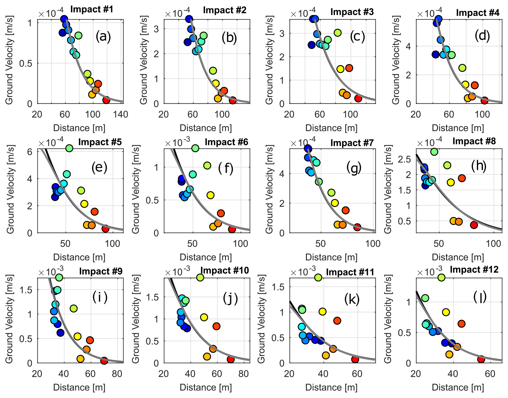
Figure 3 Maximum envelope amplitude as a function of the distance for each impact and each geophone for Block 1. The colour corresponds to the colour of the geophones in Fig. 1. The black line indicates the best regression computed with the model assuming a signal dominated by surface waves (Eq. 1), and the dark-grey line assumes a signal dominated by body waves (Eq. 2).

3.2 Correlations between the seismic and trajectography parameters

For 298 impacts we analyse the relationship between two seismic quantities (A₀ and E_S) and nine kinematic parameters: the incident northbound, eastbound, and vertical velocity and the incident velocity modulus (Vix, Viy, Viz, and |Vi|); the incident and the rebound momentum (Pi and Pf); the incident and rebound kinetic energy (E_i and E_f); and the difference between those two energies (E_f − E_i). The x axis is oriented east to west, and the y axis is oriented south to north. For each pair, we tested simple linear regressions and computed determination coefficients (Fig. 4).

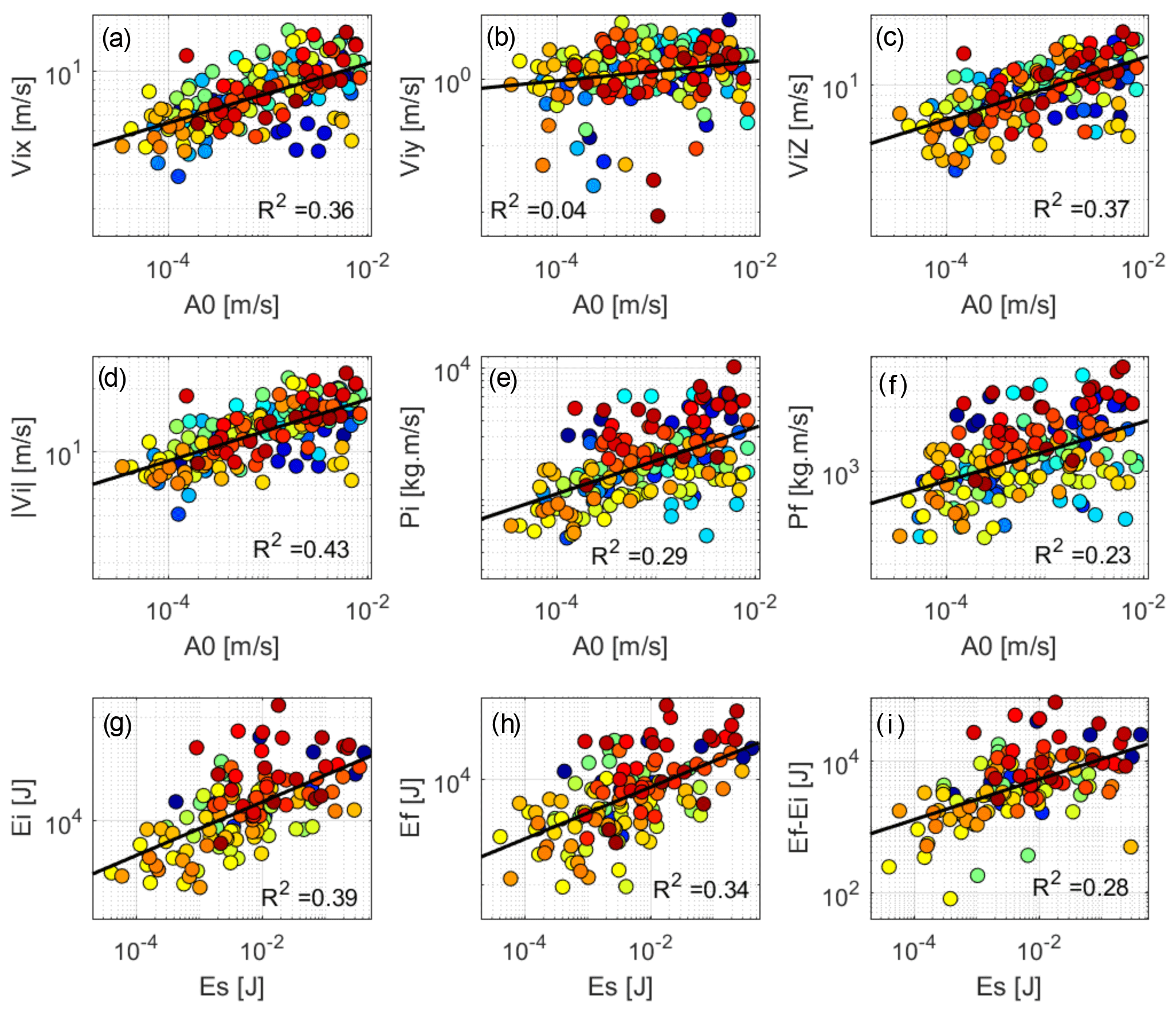
Figure 4 Correlation between the seismic and trajectography properties of the blocks: (a) the eastbound incident velocity; (b) the northbound incident velocity; (c) the vertical incident velocity; (d) the modulus of the incident velocity; (e) the incident total momentum; (f) the restituted momentum as a function of the maximum amplitude at the source A₀; and (g) the incident kinetic energy, (h) the restituted kinetic energy, and (i) the difference of both as a function of the seismic energy E_s. The black line indicates the best linear regression, with the coefficient of determination R² indicated in the panel. Dots of the same colour are from the same rockfall launch (i.e., identical block mass). Confidence intervals are not shown as they are too large.

The best correlations are observed between the incident velocity modulus |Vi| and the maximum amplitude at the source A₀ and between the incident kinetic energy E_i and the seismic energy E_s, with a determination coefficient R² of 0.43 and 0.39 respectively. The worst correlation is observed between the northbound velocity and A₀ with an R² of 0.04.

3.3 Mass and velocity predictions

We assessed the quality of the predicted results by computing the difference in percent between the predicted and the measured values of the block mass and of the modulus of the velocity inferred from the kinematic reconstruction presented in Noël et al. (2022). Therefore a difference of 0 % is reached when the predicted value is equal to the real value. In Table 1 we present the median error of the prediction on the 100 instances of training and testing the algorithm as a function of the number of samples used to train the model (10 to 100). The median values, which are less impacted by outlier values, are reported in Table 1. The mean, the median, and the complete distribution of the error on the prediction of the mass and the velocity for the cases of model training with 10 to 100 samples are presented in Fig. 5.

Table 1 Prediction results: percentage of error between the real and the predicted values

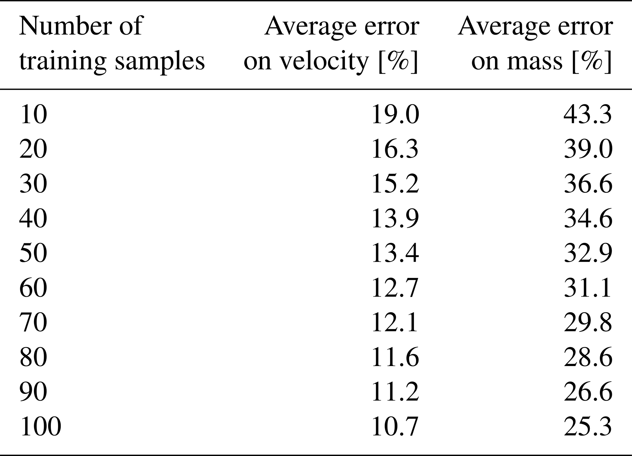
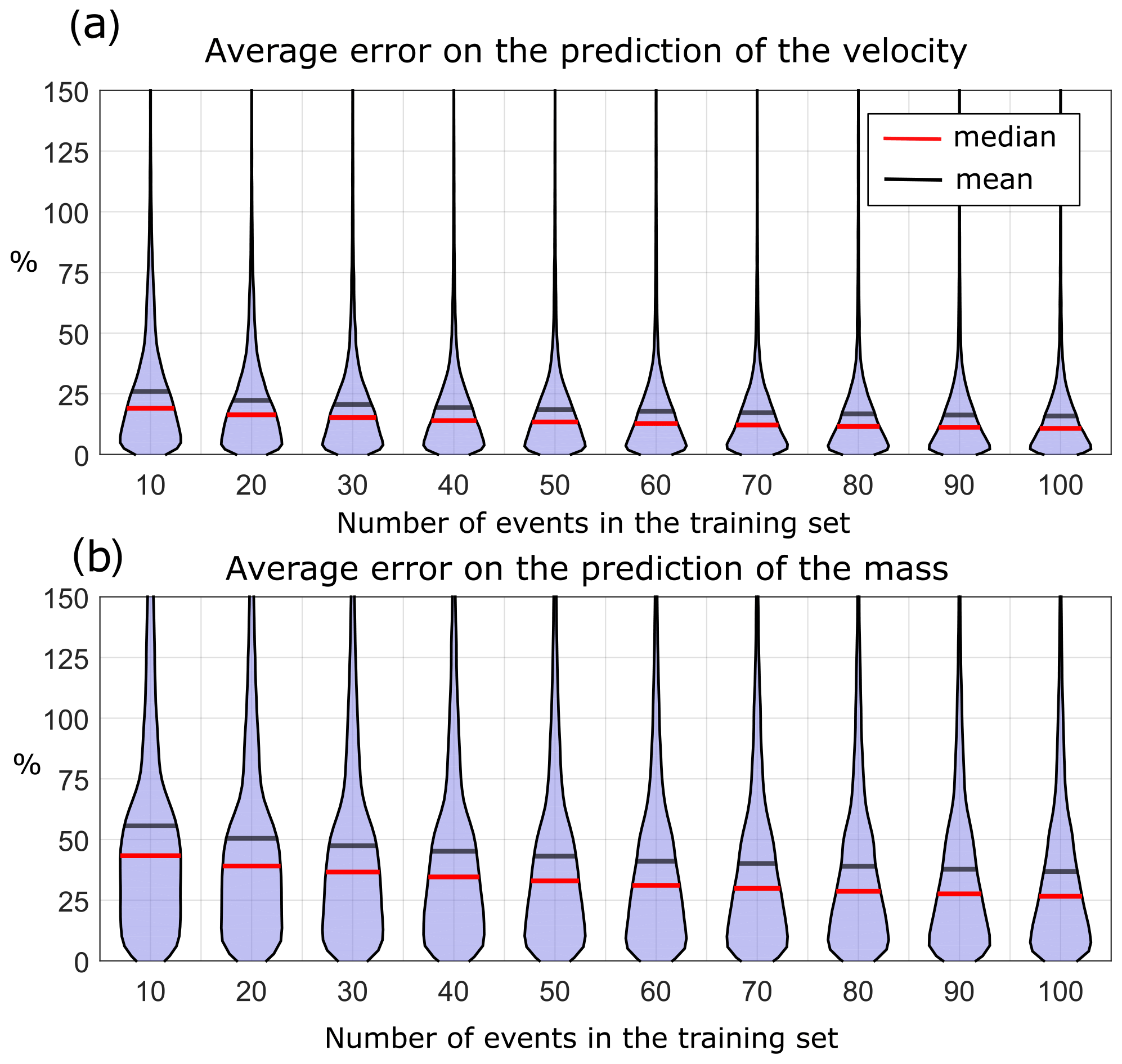
Figure 5 Distribution of the error (%) over 100 instances of training and testing the random forest model for the prediction of the mass values when trained with 10 to 100 samples to predict (a) the velocity and (b) the mass. The mean error is indicated by a black line, and the median is indicated by a red line.

As shown in Table 1 and Fig. 5, with 10 samples used to train the model, we reach a median of the prediction error of 43.3 % on the mass and 19.0 % on the velocity. Those values drop to 32.9 % and 13.4 % for 50 samples and to 25.3 % and 10.7 % for 100 samples. When training the model with 10 samples we underestimate the mass (the predicted mass is lower than the real mass) for 39.8 % of the events, and we underestimate the velocity for 49.0 % of the events. When training the model with 50 samples we underestimate the mass for 37.6 % of the events, and we underestimate the velocity for 49.6 % of the events, and when training with 100 samples we underestimate the mass for 38.0 % of the events, and we underestimate the velocity for 48.9 % of the events.

3.4 Feature importance

Figure 6 presents the mean importance scores of the features for models aiming at predicting the mass and the velocity and trained with 100 samples. For the mass prediction, the 20 best features are based on the waveforms (8 features) and the pseudo-spectrograms (11 features). Only 1 spectral feature appears in the top 20. The 5 most important features are the mean of the seismic energy in the 5–10 Hz frequency band (no. 13), the mean of the seismic energy in the 10–30 Hz frequency band (no. 14), the mean ratio between the envelope of the maximum frequency over the envelope of the mean frequency (no. 43), the mean ratio between the envelope of the second quartile of the frequency spectrum over the envelope of the first quartile of the frequency spectrum (no. 55), and the mean ratio between the envelope of the third quartile of the frequency spectrum over the envelope of the first quartile of the frequency spectrum (no. 57).

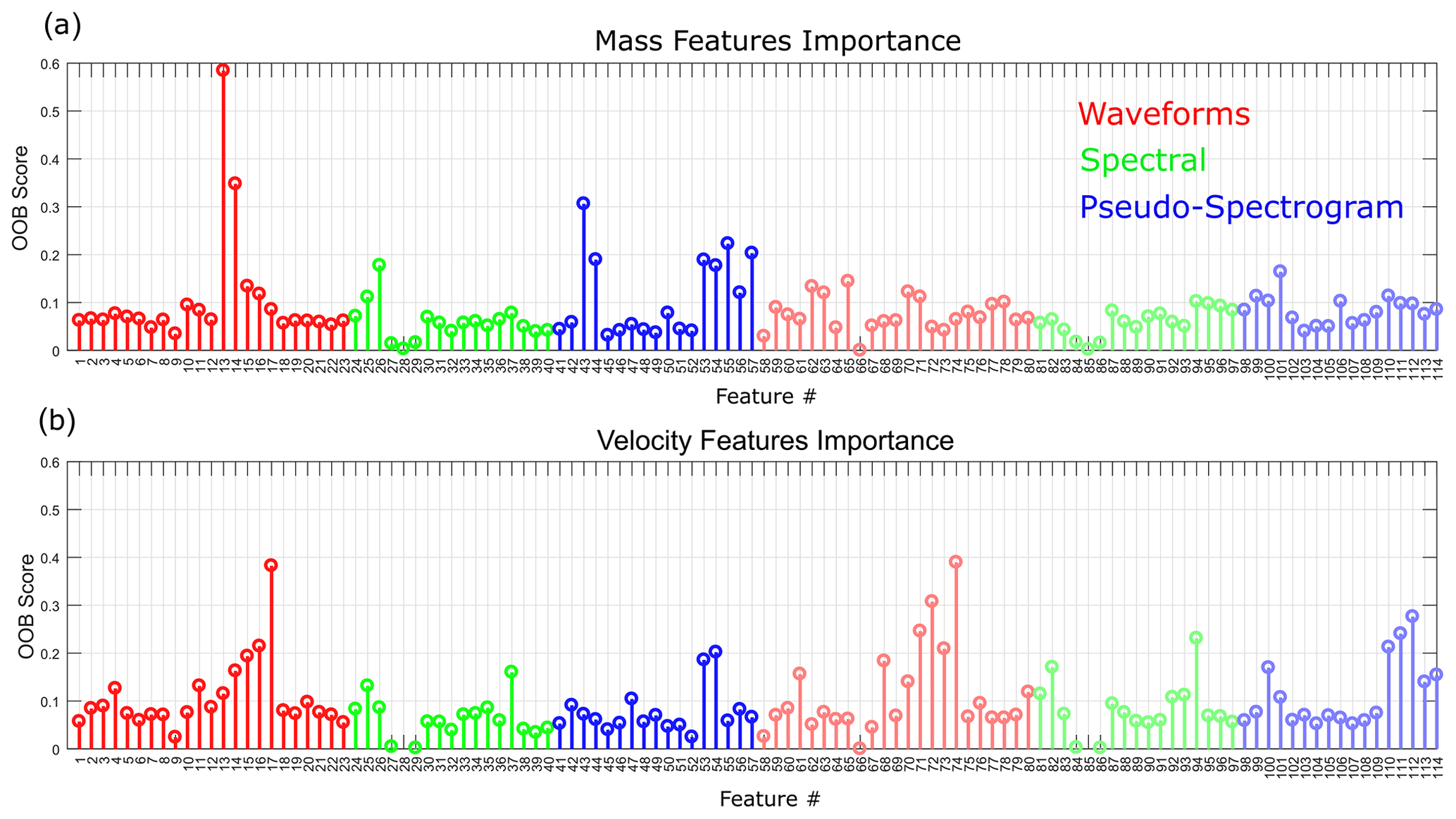
Figure 6 Importance score of the features for the prediction of (a) the mass and (b) the velocity. Colours indicate the family of features (waveform, spectral, or pseudo-spectrogram). Bright colours correspond to the mean of the features, while dimmed colours correspond to the standard deviation of the features. The description of each feature and their respective numbers can be found in Appendix A.

For the velocity prediction, the 20 best features are also mostly based on the waveforms (10 features) and the pseudo-spectrograms (7 features), with only 3 spectral features appearing in the top 20. The 5 most important features are the standard deviation of the seismic energy in the 100–200 Hz frequency band (no. 74), the mean of the seismic energy in the 100–200 Hz frequency band (no. 17), the standard deviation of the values of the energy of the seismic signal in the 50–100 Hz frequency band (no. 72), the standard deviation of the difference between the envelope of the maximum frequency over the envelope of the median frequency (no. 111), and the standard deviation of the values of the energy of the seismic signal in the 30–50 Hz frequency band (no. 71).

We can note that (1) none of the best 5 features are the same for the mass and the velocity prediction; (2) only 6 features are common in the top 20 for both quantities; and (3) mass prediction uses none of the features computed from the standard deviation of the features computed at each station (features with numbers above no. 57), while the model for velocity prediction uses 4 of them in the top 5. Finally, most of the top 5 features for the mass and the velocity prediction are based on a difference of energy in several frequency bands.

4 Discussion

4.1 Correlations between the seismic and trajectography parameters

Figure 4 shows qualitative correlations between the momentum, the kinetic energy, the maximum amplitude at the source, and the seismic energy, as observed or modelled in previous studies (Deparis et al., 2008; Vilajosana et al., 2008; Hibert et al., 2011; Levy et al., 2015; Farin et al., 2015; Hibert et al., 2017b; Farin et al., 2016; Saló et al., 2018; Le Roy et al., 2019). Our results suggest that the kinetic energy before impact is better correlated to the seismic energy than the loss of kinetic energy between the impact and the rebound E_f−E_i. The block travel directions were mostly from west to east along the gully morphology. The lack of strong displacement in the north–south direction, and hence the low velocity values, might explain the poorest correlation observed between Viy and A₀.

However, most R² values are low for all the correlations investigated. Those weak quantitative correlations precluded us from using the scaling laws to estimate the mass and the velocity of the blocks at each impact as proposed in Hibert et al. (2017b) because it would result in very high uncertainties on the inferred masses and velocities. As demonstrated by Kuehnert et al. (2020a), velocity–depth profile, 3D soil heterogeneities, source direction, and the topography play a major role in the modulation of the waveforms and the amplification of both the maximum amplitude and the energy of the generated seismic signals. Those effects are not taken into account in the simple attenuation models used in this study and numerous previous ones. We are starting to have access to complex models that can take into account some of these effects for high-frequency seismic signals (Kuehnert et al., 2020a), but they require high computational time and a comprehensive knowledge of the context physical properties (velocity profile, 3D medium heterogeneities, etc.), which can be difficult to get for real conditions. Having access to these models to perform direct modelling or inversion of the source parameters might be laborious and expensive to reproduce in different contexts, preventing a hypothetical easy portability of the approach for operational uses. This motivated the exploration of the machine learning approach to infer the properties of the rockfall without needing any attenuation model or an a priori knowledge of the medium.

4.2 Seismic signal features importance and physical model

The force imparted by an elastic sphere on a solid elastic surface can be described by the Hertz contact theory (Hertz, 1882), as proposed by (Farin et al., 2015), and was demonstrated to be relevant to model the force created by a block impacting the ground in experimental and natural experiments (Farin et al., 2015; Bachelet et al., 2018; Kuehnert et al., 2020a). These studies have shown that, in the framework provided by the Hertz theory, the seismic signal's maximum amplitude, energy, corner frequency, or the variance of the spectra is controlled by the velocity, the mass, the duration of the impact, and the physics and the geometry of the contact of a single block with the ground. Therefore the seismic signal's maximum amplitude, energy, corner frequency, or spectrum variance carries information on the dynamics and properties of the impacting block and might be analysed to retrieve those physical quantities and especially the force, the velocity, and the mass of the impactor.

The random forest model we trained yields information on which features of the seismic signal carry the most important information to successfully predict the mass and the velocity. We observe that the most important features used to predict the velocity are not exactly the same as those used to predict the mass. However, the absolute seismic energy in several frequency bands (features 13–17 and 70–74) is an important piece of information for both the prediction of the mass and of the velocity. This is consistent with the works by, e.g., Huang et al. (2007); Farin et al. (2015); Hibert et al. (2017b) and Kuehnert et al. (2020a), which have shown that the radiated seismic energy and the frequency content of a seismic signal generated by an individual impactor scales with its mass and velocity. Hence, by including the energy of the seismic signal filtered in different frequency bands as features in our predictive model, we can retrieve this correlation and allow the model to make accurate predictions.

We have observed a discrepancy in the importance of the features used for predicting mass and velocity in a specific set of features (13–17 and 70–74). While the standard deviation of feature values has a significant impact on the prediction of velocity, it does not affect the prediction of mass. This suggests that differences in seismic energies recorded at different stations are crucial for predicting velocity but not mass. Additionally, energy in lower-frequency bands plays a significant role in predicting mass, while energy in the highest-frequency band is important in predicting velocity, as indicated by features 37 and 94. Due to the attenuation of high-frequency seismic waves during propagation, seismic signals recorded at closer stations may be more important in determining velocity. However, the details of this process and why it only affects velocity prediction are difficult to understand from our dataset and require further investigation, such as through laboratory experiments. This observation is not inconsistent with the Hertz theory.

Regarding the frequency content, according to the feature importance, the full spectrum (FFT) of the whole signal carries less information than the spectrograms and the filtered waveforms. This is unexpected, as, according to the Hertz theory, the full spectrum of the signal (maximum amplitude, variance, and corner frequency) should all be highly dependent on the mass and the velocity of the impactor. This suggests that the temporal variation in the seismic signal spectrum (i.e., spectrograms) is more important in the prediction process and hence carries more information on the source properties than the information we can obtain from the full frequency spectrum itself.

We found that with the 114 selected features, our machine learning model more accurately predicts the velocity of the block at impact than its mass. According to a study by Kuehnert et al. (2020a) on real rockfalls at the Piton de la Fournaise volcano, the maximum impact force and the resulting seismic signal amplitude are highly sensitive to variations in impact speed, while the frequency content of the seismic signal is most sensitive to the density and Young's modulus of the impactor and impacted plane. Given that all blocks and impacted zones had similar elastic properties in our study, it is likely that the variability in impacted forces and the resulting seismic signals were primarily influenced by changes in velocity rather than mass. This could help to explain why features based solely on the frequency spectrum of the seismic signals appeared to be less important in our regression analysis than those containing information on the amplitude of the seismic signals. Therefore, we think that in our case the seismic signal feature range is primarily influenced by changes in velocity rather than mass, making it easier for our machine learning model to predict velocity and potentially explaining some of our earlier findings.

5 Conclusions and perspectives

From the experimental single-block controlled launches conducted in the Riou Bourdoux torrent, we demonstrated that a machine learning model based on the random forest algorithm is able to provide an estimate of the mass and the velocity of the block at each impact with an average error of around 25 % for the mass and 10 % for the velocity. With this new approach, we obtain a prediction accuracy on these two quantities equivalent to or better than all previous studies focusing on the high frequencies of the seismic signals generated by mass movements, which gave errors ranging from 20 % to 400 % of the target values (e.g., Hibert et al., 2011; Dammeier et al., 2011; Farin et al., 2015; Hibert et al., 2017b; Le Roy et al., 2019).

The machine learning model solely uses the features of the recorded signals and does not require an attenuation model to estimate the source properties conversely to the approaches based on the computation of the seismic energy and the maximum amplitude at the source. This removes the need to make assumptions which are necessary in the classical approaches used until now but which carry strong uncertainties, such as the velocity of the seismic waves, the density of the soil, the anelastic attenuation factor, and the attenuation model used. The machine learning approach also removes the need to know the exact localisation of the impacts and to correct for site effects. Those are major advantages for an operational implementation of such methods for rockfall risk assessment and mitigation. An implementation in any context will only require us to perform several well-monitored, controlled launches of rockfalls to produce a dataset to train the machine learning model, which will then be able to predict the mass and the velocity of future rockfalls. Another strength of the random forest approach is its ability to perform well even with few events used to train the algorithm. Finally, we use the same seismic signal features to predict the mass and the velocity of rockfalls that are already used to detect and identify seismic sources associated with mass-wasting processes (Provost et al., 2017; Hibert et al., 2017c; Maggi et al., 2017; Wenner et al., 2021). This opens the possibility of building a detection system, based on seismic waves, which is able to tell when a rockfall occurs and what its mass and velocity and possibly its localisation are, all at the same time and even in near-real time, given the possibility to easily record and broadcast seismic data.

It is further important to note that this experiment was performed in a controlled context with an ideal setup, with simple mono-block rockfalls which travelled roughly along the same path, and with a seismic network very close to the sources. The transferability of the machine learning model trained in our experiment may pose challenges, but the transferability of the approach itself is relatively straightforward. In our study, we utilised an extensive array of sensors to gather precise data on the dynamics of the blocks and their seismic signals. However, for practical implementation for monitoring purposes, one would only need to deploy a seismic sensor network and launch 10 to 30 blocks into the network to acquire sufficient data for training a model capable of predicting the mass of the blocks. To predict velocity, additional field work would be required, such as utilising a mobile GNSS to determine the impact positions of each block and calculating their velocities. Alternative approaches based on physical models would demand similar efforts, especially in calibrating scaling laws, but would also necessitate a robust attenuation model of the medium through seismic tomography and an accurate method of localising impacts for each new event, potentially resulting in lower accuracy. One of the advantages of the random forest approach is that it does not rely on an attenuation model or impact localisation to estimate block mass and velocity. Our approach shows its ability to retrieve source properties for a wide range of geophone impact distances. However, the influence of network geometries and the minimum number of stations needed to get accurate estimates have to be assessed in future experiments. Those future experiments will also help to study the transferability of trained models and eventually lead to proposing an operational system for detecting, classifying, and characterising the properties of rockfalls that would integrate machine learning approaches for near-real-time monitoring.

The machine-learning-based approach must now be experienced with more complex sources, such as multi-block rockfalls and even granular flows, and with more distant seismic stations. The station distances might hinder the ability of the machine learning model to estimate source properties, as the farthest we are from the source, the more we lose information due to propagation effects on seismic waves. However, the recent successes (Provost et al., 2017; Hibert et al., 2019; Wenner et al., 2021; Chmiel et al., 2021) in identifying mass-wasting sources at medium to long distances, with the same approach and the same features, suggest that even when recording seismic signals far from the source, seismic signals retain information on the source properties in the higher-frequency band (above 1 Hz) that could allow us to determine those properties using the same approach. This would be a major breakthrough, as it would allow us to determine source properties for most landslides which do not generate seismic waves with enough energy in the lowest-frequency bands to allow for an inversion of the properties of the source. This will be the subject of future work.

Finally, this approach based on machine learning algorithms might be applied to the analysis of other environmental processes for which classical seismological source inversion methods are not suitable. This could be used for the determination of properties (mass, velocity, flux, volume, forces, momentum, etc.) of sources that generate tremors (volcanic eruptions, debris flows and intense storms), complex high-frequency and even low-frequency signals (ice-calving events and hydro-acoustic signals), or even anthropogenic noises (vehicles and pumps). However, as for every machine-learning-based approach, sets of calibrated and well-known examples are necessary to train the models. Physical models can also help by producing physically based synthetic seismic signals. Regression of seismic source properties using machine learning approaches is a new complementary and interesting tool for the community interested in exotic or environmental seismic sources relevant for improving our understanding of these processes.

Appendix A

Table A1 Feature table.

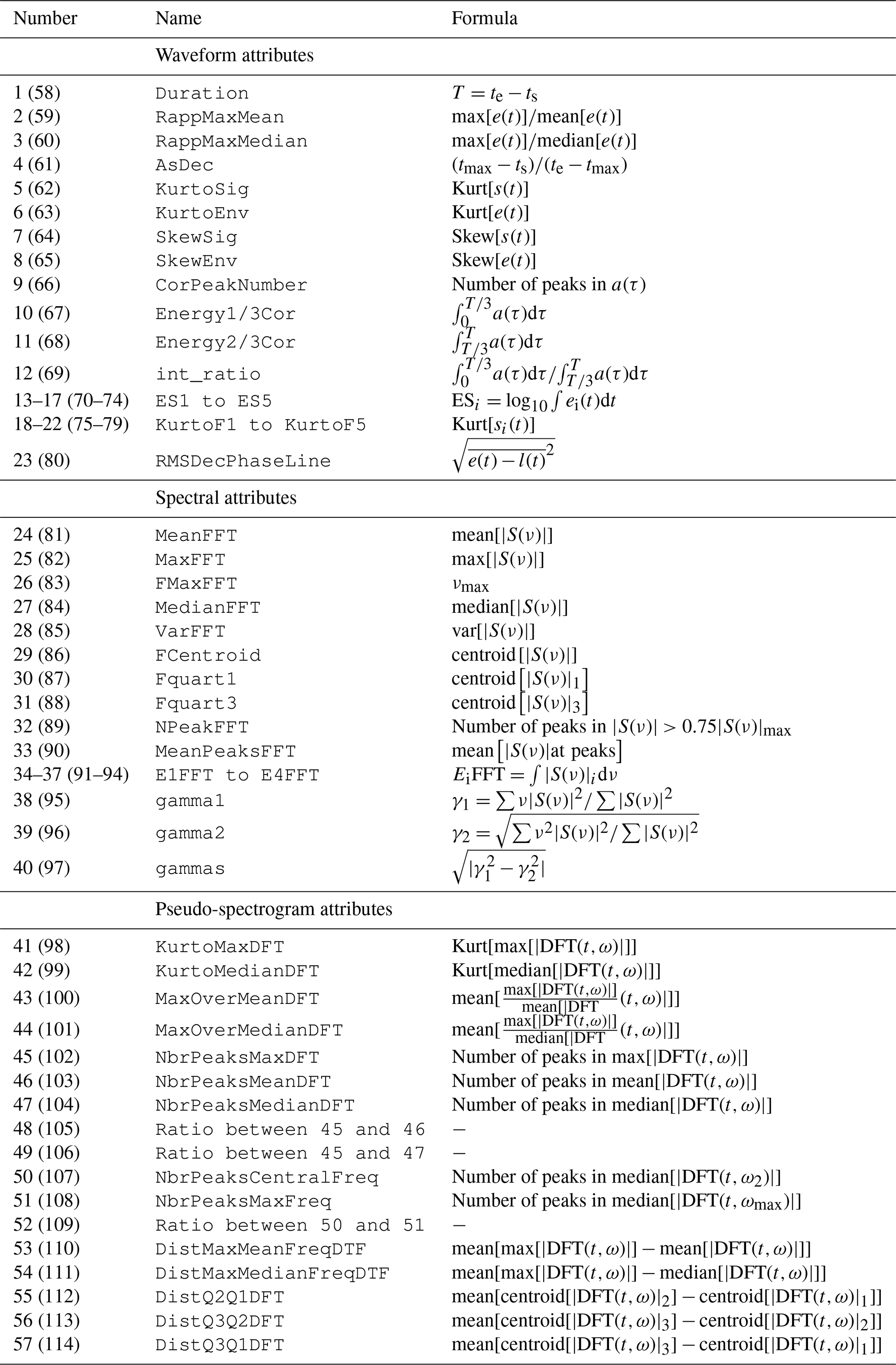
Number for standard deviation of feature is given in parentheses. Waveform- and spectrum-based features, with s(t) as the windowed raw seismogram; e(t) as its envelope; $l\left(t\right)=e_{\max }-\frac{e_{\max }}{t_{\mathrm{f}}-t_{\max }}t$, a(τ) as its auto-correlation function; s_i(t) as the windowed seismograms filtered in the 5–10 Hz (i=1), 10–30 Hz (i=2), 30–50 Hz (i=3), 50–100 Hz (i=4), and 100–199 Hz (i=5) frequency bands; e_i(t) as their corresponding envelopes; t_s and t_e as the start and end times of the window; t_max as the time of the maximum amplitude; $\mathrm{Kurt}\left(X\right)=\frac{{\mathit{\mu }}_{\mathrm{4}}\left(X\right)}{{\mathit{\sigma }}^{\mathrm{4}}\left(X\right)}$ as the Kurtosis of distribution X where μ₄(X) indicates the fourth moment of X and σ indicates its standard deviation; $\mathrm{Skew}\left(X\right)=\frac{{\mathit{\mu }}_{\mathrm{3}}\left(X\right)}{{\mathit{\sigma }}^{\mathrm{3}}\left(X\right)}$ as the Skewness of distribution X where μ₃ indicates the third moment of X; S(ν) as the fast Fourier transform of s(t); ν_max as the frequency at which $\left|S\right(\mathit{\nu }\left)\right|$ is at its maximum; $\left|S\right(\mathit{\nu }){|}_i$ as the ith quartile of $\left|S\right(\mathit{\nu }\left)\right|$; DFT(t,ω) as the discrete Fourier transform of s(t); ω₂ as the central frequency of DFT(t,ω); ω_max as the frequency at the maximum of DFT(t,ω); and |DFT$(t,\mathit{\omega }){|}_j$ as the jth quartile of |DFT$(t,\mathit{\omega })|$.