the Creative Commons Attribution 4.0 License.
the Creative Commons Attribution 4.0 License.
 | 15 May 2024
3D shear wave velocity imaging of the subsurface structure of granite rocks in the arid climate of Pan de Azúcar, Chile, revealed by Bayesian inversion of HVSR curves
Rahmantara Trichandi
Klaus Bauer
Trond Ryberg
Benjamin Heit
Jaime Araya Vargas
Friedhelm von Blanckenburg
Charlotte M. Krawczyk
Seismic methods are emerging as efficient tools for imaging the subsurface to investigate the weathering zone. The structure of the weathering zone can be identified by differing shear wave velocities as various weathering processes will alter the properties of rocks. Currently, 3D subsurface modelling of the weathering zone is gaining increasing importance as results allow the identification of the weathering imprint in the subsurface not only from top to bottom but also in three dimensions. We investigated the 3D weathering structure of monzogranite bedrock near the Pan de Azúcar National Park (Atacama Desert, northern Chile), where the weathering is weak due to the arid climate conditions. We set up an array measurement that records seismic ambient noise, which we used to extract the horizontal-to-vertical spectral ratio (HVSR) curves. The curves were then used to invert for 1D shear wave velocity (Vs) models, which we then used to compile a pseudo-3D model of the subsurface structure in our study area. To invert the 1D Vs model, we applied a transdimensional hierarchical Bayesian inversion scheme, allowing us to invert the HVSR curve with minimal prior information. The resulting 3D model allowed us to image the granite gradient from the surface down to ca. 50 m depth and confirmed the presence of dikes of mafic composition intruding the granite. We identified three main zones of fractured granite, altered granite, and the granite bedrock in addition to the mafic dikes with relatively higher Vs. The fractured granite layer was identified with Vs of 1.4 km s−1 at 30–40 m depth, while the granite bedrock was delineated with Vs of 2.5 km s−1 and a depth range between 10 and 50 m depth. We compared the resulting subsurface structure to other sites in the Chilean coastal cordillera located in various climatic conditions and found that the weathering depth and structure at a given location depend on a complex interaction between surface processes such as precipitation rate, tectonic uplift and fracturing, and erosion. Moreover, these local geological features such as the intrusion of mafic dikes can create significant spatial variations to the weathering structure and therefore emphasize the importance of 3D imaging of the weathering structure. The imaged structure of the subsurface in Pan de Azúcar provides the unique opportunity to image the heterogeneities of a rock preconditioned for weathering but one that has never experienced extensive weathering given the absence of precipitation.
- Article
(10988 KB) - Full-text XML
- BibTeX
- EndNote


Weathering can modify the mineralogy of rocks, resulting in petrophysical changes that can be detected with geophysical methods. Numerous geophysical imaging techniques have been successfully applied to characterize the weathering structure in granitic rocks, including the use of electrical resistivity tomography (Olona et al., 2010; Holbrook et al., 2014), ground-penetrating radar (GPR) (Dal Bo et al., 2019), and seismic tomography (Trichandi et al., 2022; Befus et al., 2011; Olona et al., 2010; Handoyo et al., 2022). These non-invasive techniques allow us to estimate the weathering structure over wide extents and/or in areas of deep weathering, where probing using traditional techniques (e.g., soil pits) is logistically expensive or can even be unfeasible.
Seismic body wave tomography is one of the most frequently used methods in weathering zone studies (Befus et al., 2011; Flinchum et al., 2018; Olona et al., 2010; Trichandi et al., 2022). The seismic signals generated by sources such as hammer, weight drop, or vibroseis are recorded by an array of seismic receivers. Seismic P-wave velocity can be inferred by the analysis and inversion of body waves' travel time. However, data acquisition of such body wave tomography experiments can be extensive as it requires the appropriate source and receiver array setup. It also restricts data acquisition in remote areas where heavy-equipment transportation can be challenging. Moreover, active seismic experiments are often not permitted in conservation areas such as national parks, where the impact of the seismic source can disturb the surrounding ecosystems.
The horizontal-to-vertical spectral ratio (HVSR) technique is a passive seismic method that does not rely on active seismic sources. It has emerged as a viable alternative to active seismic methods for effectively imaging the subsurface weathering zone. The HVSR method was initially applied for site characterization in seismic hazard assessment (Piña-Flores et al., 2020; Mahajan et al., 2012) and imaging of sedimentary basins (Cipta et al., 2018; Pastén et al., 2016; Koesuma et al., 2017; Pilz et al., 2010). More recently, the HVSR method has been utilized at smaller scales for investigating bedrock (Maghami et al., 2021; Moon et al., 2019; Nelson and McBride, 2019; Trichandi et al., 2023). This approach has gained popularity due to its simplicity, rapid data acquisition, and ease of placing measurement points. However, it is important to note that the inverse problem associated with the HVSR curve is highly non-linear and necessitates prior knowledge of the subsurface structure (Moon et al., 2019; Nelson and McBride, 2019; Pilz et al., 2010).
Utilizing a transdimensional and hierarchical Bayesian Markov chain Monte Carlo (MCMC) approach solves the prior information requirement challenge in HVSR curve inversion. This approach is beneficial as it only requires minimal prior information about the subsurface structure during the inversion process (Ryberg and Haberland, 2019; Trichandi et al., 2022). Moreover, the transdimensional approach allows changes in dimensionality throughout the inversion, eliminating the need for prior constraints on determining the number of layers (Cipta et al., 2018; Bodin, 2010; Bodin et al., 2012). Consequently, this procedure reduces uncertainty levels and provides a robust, data-driven shear wave velocity (Vs) model that can be readily interpreted.
In this paper, we explore the shallow (< 50 m) subsurface structure of granite bedrock in the arid climate near the Pan de Azúcar National Park, which is one of the test sites of the “EarthShape (Earth surface shaping by biota)” project that covers the Chilean climate gradient from dry to humid (Oeser et al., 2018; Oeser and von Blanckenburg, 2020). In this study, we apply the HVSR method combined with the Bayesian inversion approach to produce a 3D subsurface image of the weathering structure around an existing borehole (−26.302717° N, −70.457350° W). Then, we compare the results with previous studies conducted at the other EarthShape test sites to further study the effects of different climate and geological processes on the deep weathering of granite.
The study was conducted on the outskirts of the Pan de Azúcar National Park, located in the Atacama Desert, approximately 200 km north of Copiapó, Chile (Fig. 1a). The area is located in the arid part of the coastal cordillera featuring very low precipitation of ∼ 10 mm yr−1 and a mean annual temperature of 18.3 °C (Karger et al., 2017; Oeser et al., 2018). With such low precipitation, the vegetation in this area is minimal and is mainly sustained by the coastal fog coming in from the Pacific Ocean (Lehnert et al., 2018). A ground-penetrating radar (GPR) study in the Pan de Azúcar National Park managed to image the subsurface down to 2 m depth, revealing an average soil thickness of 0.20 m (Dal Bo et al., 2019). Information from a greater depth was not obtained due to the frequency limitation (Dal Bo et al., 2019).
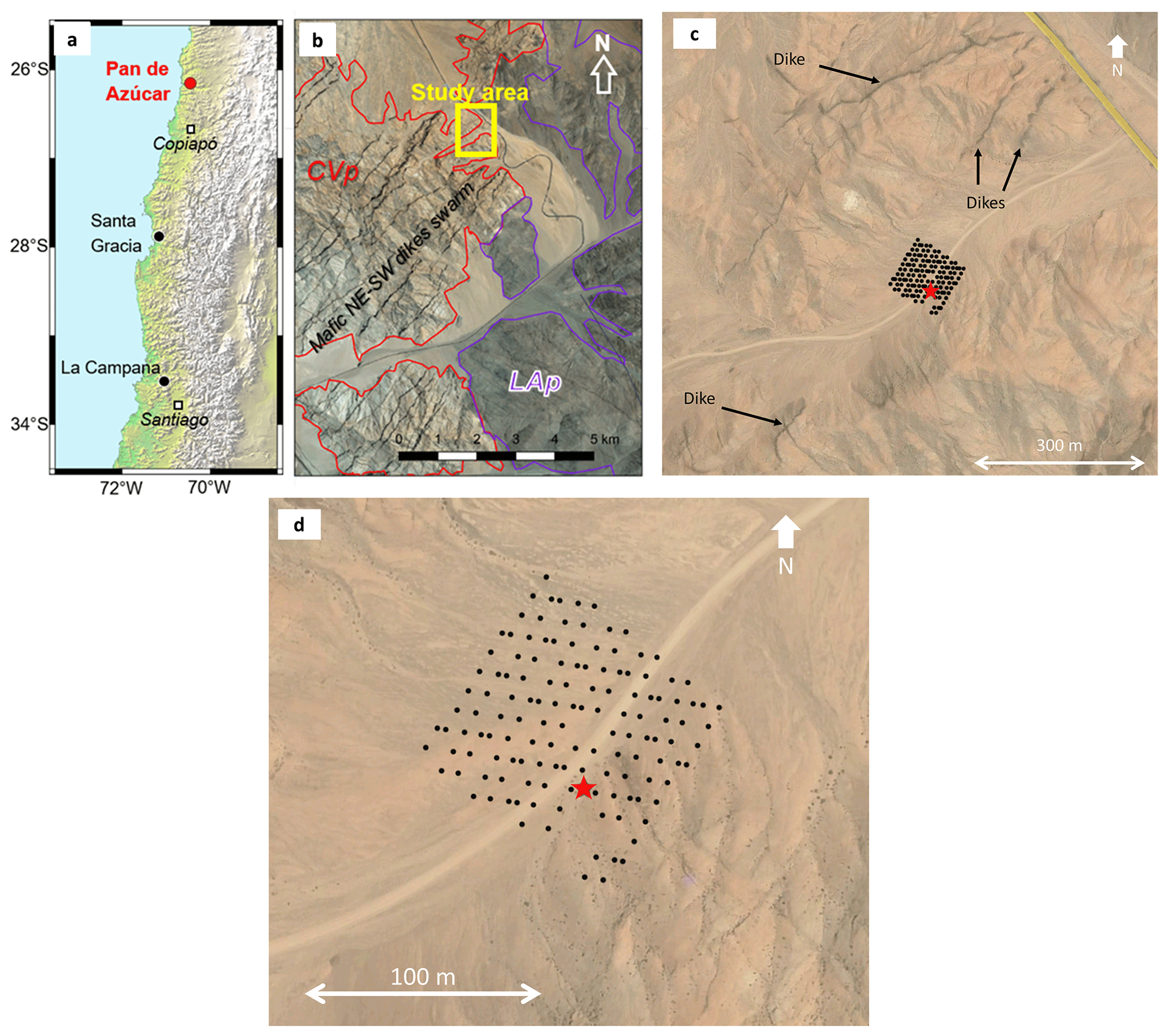
Figure 1Information on the Chile Pan de Azúcar study site. (a) Study site location. (b) Local geology information of the study area (Sernageomin, 1982). Red and purple lines outline the Cerros del Vetado (CVp) and Las Ánimas (LAp) plutons, respectively (modified from Godoy and Lara, 1998). (c) Google Earth image of the study site (© Google Earth 2019). Some of the mafic dikes outcropping in the area are highlighted. (d) Seismic array. Black dots in panels (c) and (d) show the positions of seismic sensors. The red star shows the location of the borehole (WGS 84 coordinates 26.30272° S, 70.45735° W) (© Google Earth 2019).
The study area is in the Triassic Cerros del Vetado pluton (Fig. 1b), comprising monzogranites and syenogranites (Godoy and Lara, 1998). Reported U–Pb ages for this pluton are in the range of 205–250 Ma (Berg and Baumann, 1985; Maksaev et al., 2014; Jara et al., 2021). Along its eastern margin, the Cerros del Vetado pluton is intruded by the Late Jurassic Las Ánimas pluton (Fig. 1b), which has reported ages in the range of 150–160 Ma (Dallmeyer et al., 1996; Godoy and Lara, 1998; Jara et al., 2021). The Cerros del Vetado pluton is also intruded by a dense network of dikes with varying directions and compositions (Berg and Baumann, 1985; Acevedo, 2022), from which a swarm of NE–SW-oriented and dark-coloured dikes of mafic (gabbroic to dioritic) composition is clearly observed in the field and crosses the study area (see dark-coloured lines in Fig. 1b and c). Dallmeyer et al. (1996) report a Ar age of 129.2 ± 0.5 Ma for one of these dikes that outcrops 8 km southwest of the study area. In 2019, a drilling campaign was conducted to investigate the weathering structure by extracting drill cores to perform core analyses. The location of the borehole is shown in Fig. 1d.
According to investigations of samples from the borehole, the bedrock at Pan de Azúcar is characterized by a high SiO2 (Ø 74 wt %), Na2O, and K2O content (> 7 wt %) and remarkably uniform major element concentrations. It comprises the major minerals of quartz, plagioclase, microcline, and biotite. The grain size distribution is relatively homogenous, with an average grain size around 0.5 cm. The granite has been hydrothermally overprinted to varying degrees. This alteration is strongest in the vicinity of large fractures. Televiewer data from the borehole revealed that the dip angles of fractures show a continuous range of dip angles between 20 and 80°. Fractures of shallower dip alternate with steeper-dipping fractures throughout the entire core. Fractures are partly cemented with calcite, clay minerals, and Fe oxides. Bedrock porosity is, with an average of around 1 %, generally low, whereas the hydrothermally overprinted core material has a bulk porosity exceeding 2.5 %. Weathering mass balances using the refractory element niobium indicated zero weathering, as expected in an arid climate. Mean soil denudation rates measured at the drill site with in situ cosmogenic 10Be measured in quartz from surface soil is 7.1 ± 0.5 t km−2 yr−1 (n=3).
We conducted a passive seismic data acquisition in Pan de Azúcar in August 2022 in a 150 × 150 m area covering the borehole location (Fig. 1c) with elevation varying between 710–750 m. The investigated area extends from gently sloping bedrock in the southeast into a colluvial valley fill consisting of sandy gravel in the northwest. The distance between measurement points was set to be 10 m apart, resulting in 225 measurement points. The ambient noise data were acquired by the subsequent deployment of 15 three-component (3-C) geophones with 4.5 Hz eigenfrequency (PE-6/B by SENSOR Nederland). Since we expected a shallow weathering structure, the 4.5 Hz eigenfrequency is deemed to be sufficient to cover the desired depth range. The geophones were planted into the ground and were connected to a CUBE data logger (DATA-CUBE3 Type 1 with internal GPS by DiGOS), which records the seismic vibrations detected by the geophones. We simultaneously deployed 15 geophones along a northwest–southeast direction line and recorded the ambient seismic noise for 1 h for each measurement point. To cover the whole area with 225 measurement points, we required 4 d of fieldwork, including the array setup.
To image the subsurface using the horizontal-to-vertical spectral ratio (HVSR) method, we first needed to process the recorded three-component noise data and extract the HVSR curve. When extracting the curves, we followed the statistical approach described by Cox et al. (2021). To guarantee sufficient data quality, we excluded the curves that did not satisfy the Site EffectS using AMbient Excitations (SESAME) guideline for site characterization (SESAME, 2004). Then, we inverted each curve using a transdimensional hierarchical Bayesian inversion approach to get a 1D Vs profile from each measurement point. We then used multiple 1D profiles to produce a pseudo-3D Vs model of the subsurface by smoothing and interpolation. A geochemical analysis of the borehole's core samples was also performed to provide a weathering indicator to the modelled Vs data.
4.1 HVSR curve extraction
The HVSR technique is a method to retrieve information about the subsurface seismic properties using a single station measurement on the surface. This was initially developed for site effect investigations (Nakamura, 1989) based on the frequency spectrum ratio of the horizontal and vertical components of a seismic recording at the same location. To extract the HVSR curves, we used the geometric mean of the frequency spectrum between the horizontal and vertical components of the seismic recording which can be described in the following equation:
where HEW(ω) and HNS(ω) are the frequency spectrums of the horizontal east–west and north–south seismic components and V(ω) is the frequency spectrum of the vertical seismic components. Sites with relatively hard and strong rock will theoretically not amplify the energy within a certain frequency band. Therefore, the ratio between the horizontal and vertical seismic components will be roughly equal. On the other hand, sites with weak and softer rocks will significantly amplify the frequency spectrum energy at a certain frequency band, resulting in a higher HVSR value (Xu and Wang, 2021). Therefore, the frequency where the HVSR curves peak can be used to determine the interface between bedrock and its overlying rocks.
Prior to the HVSR curve extraction process, we applied instrumental correction and a 1.0 to 150 Hz bandpass filter to the three components' raw data (vertical, east–west, and north–south). We used 60 min of ambient noise for each point, as shown by the example in Fig. 2a–c. The time series data were then transformed into a frequency domain by the application of a straightforward Fourier transform (Fig. 2d–f). To improve the quality and stability of our HVSR curve, we followed the statistical approach of HVSR curve extraction described by Cox et al. (2021). We divided the time series data into 60 s time windows and rejected time windows that exceeded a statistical threshold of peak frequency and variance. This windowing approach will reject time windows which result in high standard deviation of the peak frequency. Therefore, high-frequency events which could contaminate the ambient noise records, such as the high-frequency and amplitude event recorded around 2800 s mark in Fig. 2a–c, will be excluded from the dataset as they will result in high standard deviation compared to the other time window. Ultimately, we obtained the final HVSR curve and the corresponding standard deviation of the HVSR curve shown in Fig. 2g.
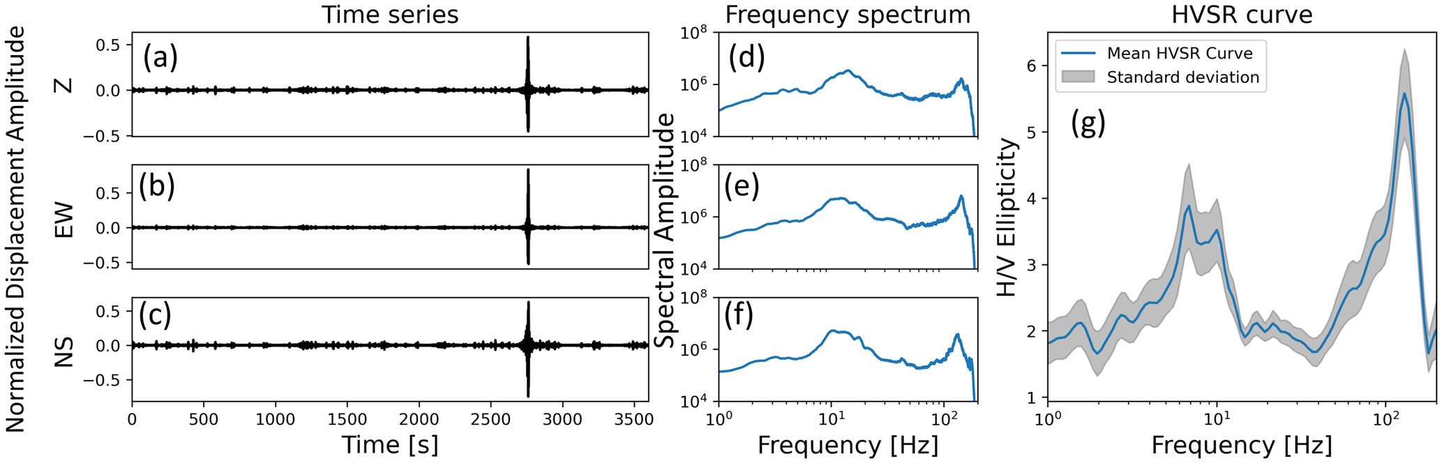
Figure 2Steps of HVSR curve extraction from a station at the borehole location (see Fig. 1d). (a–c) 60 min three-component time-domain-normalized seismic noise recordings. (d–f) The respective frequency power spectrum. (g) The resulting HVSR curve extracted using the hvsrpy package (Vantassel, 2020).
After extractions of the HVSR curve from all the observation points, we checked for the HVSR curve's consistency. Colour plots of the HVSR curve in Fig. 3a reveal mainly two frequency ranges with peak frequencies of below 30 Hz and around 100 Hz. Since the study is more focused on the boundary between the bedrock and its overlying weathering structure, the higher-frequency data will later be discarded as the HVSR curve peak around 100 Hz is often associated with the boundary between soil and saprolite (Nelson and McBride, 2019). The HVSR curve with high uncertainties was also discarded. An average of all the HVSR curves is shown in Fig. 3b, where it is possible to observe various frequency peaks in the frequency range lower than 10 Hz, which could be related to the varying bedrock depth.
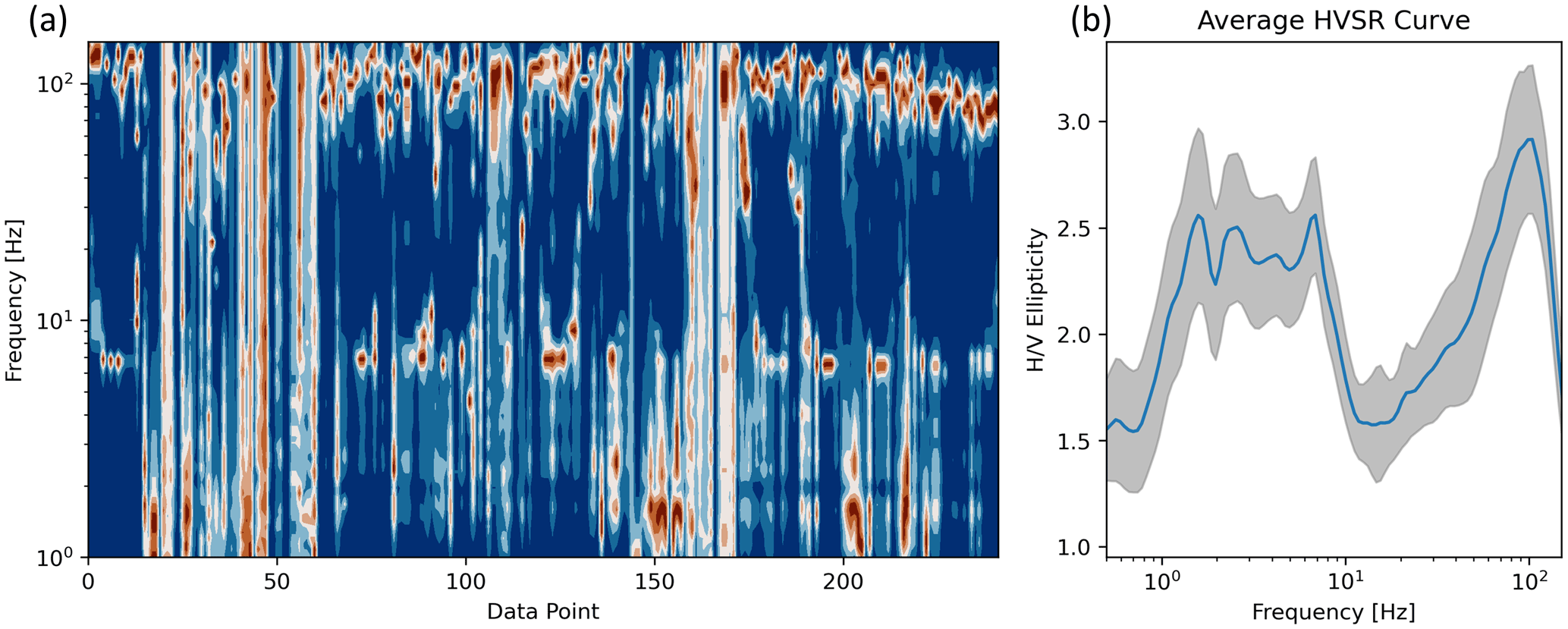
Figure 3Collection of the extracted HVSR curve in the survey area (a) and the mean HVSR curve (b).
4.2 HVSR curve inversion
The substantial non-uniqueness inherent in HVSR curve modelling introduces a highly non-linear inverse problem. Various approaches have been employed to address this challenge, including the implementation of a least-squares approach (Arai and Tokimatsu, 2004), fixing the number of layers (Fäh et al., 2003; Parolai et al., 2005; Hobiger et al., 2013; Wathelet et al., 2004), and fixing the bedrock velocity (Parolai et al., 2005). These approaches tried to simplify the inverse problem by incorporating prior information about the true model into the inversion process. For instance, it is often difficult to determine the expected number of layers without preliminary subsurface investigations in the context of investigating weathering zones. As for fixing the bedrock velocity, although previous research on similar bedrock formations can provide some prior knowledge about the velocity, it is common for bedrock velocities to vary between different sites (Trichandi et al., 2023, 2022). Furthermore, reliably fixing the bedrock velocity would necessitate accurate bedrock P- and S-wave velocity information.
For the inversion workflow, we followed the transdimensional hierarchical Bayesian Markov chain Monte Carlo (MCMC) inversion scheme as described by Bodin (2010), which had also been applied to the HVSR curve inversion (Cipta et al., 2018; Trichandi et al., 2023). The main advantage of using this inversion scheme is that we require only minimal prior information about the real model (Ryberg and Haberland, 2019; Trichandi et al., 2022). With this inversion routine, we do not need to fix the bedrock velocity as it will be determined during the inversion process. Furthermore, with the transdimensional approach, we do not have to define a fixed number of layers for our model, as the number of layers will be determined during the inversion process based on the data noise level.
For the parameterization of the inversion, we defined a wide range of values for each parameter. The Vs value was determined to be between 0.1 and 5.0 km s−1 to accommodate the possible existence of very loose material, such as soil with low velocity or even intruding solid-rock layers with very high velocity. The advantage of using a relatively large model space is also to allow the inversion scheme to explore the whole model space and not be trapped in a local minimum. For the number of layers, we also enabled the inversion to explore models with a number of layers between 2 and 20 layers (including half-space). As for the input data, we limit the observed HVSR curve to be between 1 and 20 Hz.
Forward calculation of the HVSR curve also requires an explicit definition of the number of layers. We accommodated the inversion to explore both simple and complex layered models by performing a transdimensional inversion approach. While the conventional approach often subdivides weathering layers into three or four layers (soil, saprolite, fractured bedrock, and bedrock), we allow the inversion to explore a simple two-layered model. This simple layered model accommodates situations where only fractured bedrock and bedrock layers are present, particularly in areas with a relatively low degree of weathering. Furthermore, this simplified model is beneficial for incorporating data with high uncertainty. Conversely, we also allowed a maximum of 20 layers to account for the possibility of highly intricate subsurface layering, acknowledging the potential complexity that may be present in certain areas.
The subsequent parameters to be determined are Vp and density. Previous studies have demonstrated that these parameters exhibit relatively low sensitivity to HVSR curve modelling and can be considered unknown nuisances during the inversion process (Cipta et al., 2018). However, for completeness, we also established uniform ranges for Vp, ranging from 0.3 to 8.0 km s−1, and for density, ranging from 1.5 to 3.0 g cm−3. It is also important to note that we did not invert the density value in our inversion and that we used the inverted Vp value to approximate the density using the equation provided by Brocher (2005).
We performed the inversion for each data point on 24 parallel Markov chains with 100 000 iterations per chain. Each chain starts by drawing a random initial model (m0) from the given prior information. The initial model is then used to model an HVSR curve () using the Geopsy forward-modelling package (Wathelet et al., 2020). The forward-calculation tool employed a model representing the subsurface as a series of homogeneous layers extending into a half-space. We used a 1D Voronoi cell approach of constant velocity layer when constructing the layered model. Then, for every iteration, one of the following perturbations was performed:
-
Perturb the data noise (σ) value according to the proposal distribution.
-
Perturb the Voronoi cell location of a random cell according to the proposal distribution. Changes in the Voronoi cell location will affect the layer's thickness of the input model.
-
Perturb the Vs value of a random cell according to the proposal distribution.
-
According to the proposal distribution, perturb a random cell's Vp/Vs value and calculate Vp accordingly for the input model.
-
Delete one random cell.
-
Add one random cell based on the prior information provided by the chain.
The perturbation process generates a new model (m1), from which we calculate the corresponding HVSR curve (dcal1). Subsequently, we determine the acceptance probability for transitioning from the initial model (m0) to the new model (m1) based on the observed data (dobs), the calculated HVSR curve of the initial model (), and the calculated HVSR curve of the new model (dcal1). We randomly decide whether to accept the transition from m0 to m1 using this acceptance probability. If the transition is accepted, m1 replaces m0, and we proceed to the next iteration. However, if the transition is not accepted, we retain m0 and move on to the next iteration. This process is repeated until the specified number of iterations is reached. The final model for each station is obtained by averaging all the accepted models from the 24 Markov chains that were executed. By averaging all the accepted models, the final model now contains information on the extensively sampled model space and can bring information that is not contained if we only use a single best-model approach (Trichandi et al., 2023). Additionally, we also include the model uncertainty by calculating the standard deviations of all the accepted models. We then use the uncertainty to limit the model depth.
4.3 Chemical depletion factor
In addition to the seismic properties, we also measured the chemical depletion factor (CDF) from the borehole's core samples. The CDF can be used to quantify the fraction of mass loss by weathering relative to the bedrock (Riebe et al., 2003; Krone et al., 2021). We calculated the CDF on core samples from the Pan de Azúcar drill core from concentrations of the insoluble element Nb in the parent rock and compared it to the Nb concentration in the weathered bedrock. The CDF was then calculated using the following equation:
where [Nb]bedrock is the Nb concentration from bedrock sample and [Nb]weathered rock is the Nb concentration from the target weathered rock sample. In Eq. (2), a positive CDF value means that the target weathered rock sample went through a depletion, while a negative CDF value means the rock went through an enrichment of the Nb concentration. For the CDF calculation in Pan de Azúcar, we compared the Nb concentration in the fractured and hydrothermally altered cores with relatively unweathered granite. An example of a strongly fractured and hydrothermally altered core can be found in Fig. 4a and c, while Fig. 4b shows relatively unweathered granite.
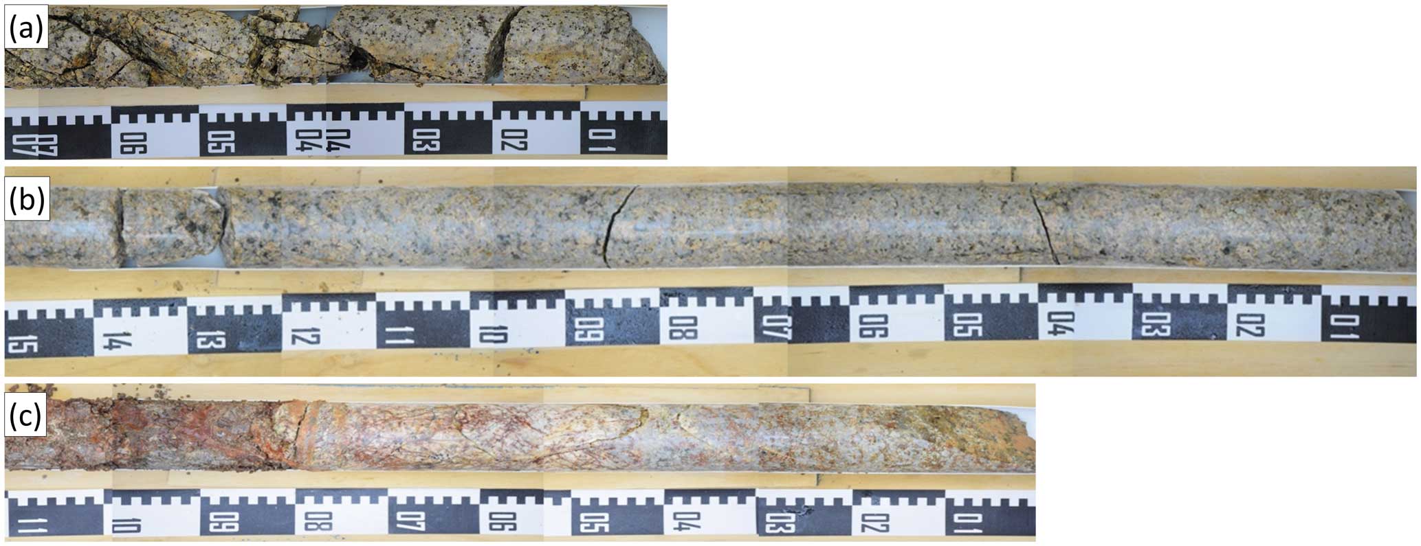
Figure 4Comparison of (a) strongly fractured and hydrothermally altered granite from 17 m core depth, (b) relatively unweathered granite from 72 m core depth, and (c) strongly hydrothermally altered granite from 86 m core depth.
We divided our results into two main parts: (1) results from the HVSR curve and (2) results from the subsequent pseudo-3D Vs model. Even before performing the HVSR curve inversion, the HVSR curve already brings an insight into the weathering zone depth as the peak frequency (f0) from the HVSR curve is often linked to the top of the bedrock depth (Nelson and McBride, 2019; Nagamani et al., 2020; Stannard et al., 2019). Using f0, we can approximate the depth of the top of the bedrock using the following equation:
where D is the depth to the top of the bedrock and Vs is the average S-wave velocity of the overlying layer. This equation shows that higher f0 is related to a shallower top-of-bedrock depth, while low-frequency f0 indicates a deeper top-of-bedrock depth. With this approximation, we can estimate the fresh bedrock depth across the study area. However, this equation highly depends on the assumption of correct Vs and therefore can only be used as an approximation.
5.1 HVSR curve frequency profile
After extracting the HVSR curves, we can determine the f0 of each HVSR curve and produce the peak frequency and apparent fresh bedrock depth map (Fig. 5a and b). The peak frequency map in Fig. 5a can be created by plotting each measurement point's peak frequency. The high frequency in Fig. 5a is related to a shallower interface between the regolith and the bedrock, while low frequency means a deeper interface as shown by the depth approximation in Eq. (1).
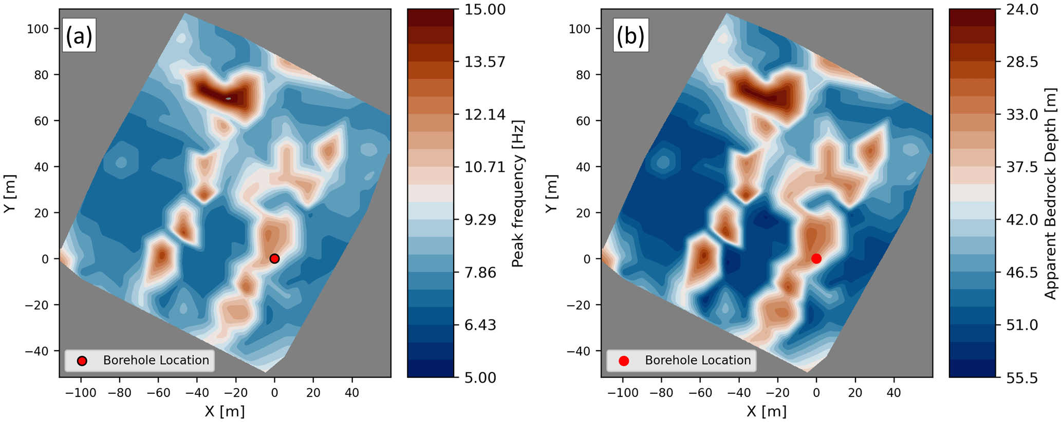
Figure 5Resulting (a) peak frequency and (b) apparent fresh bedrock depth map assuming Vs = 1.50 km s−1. The red dot represents the borehole location. Higher frequency in panel (a) is related to a shallower bedrock, while, inversely, lower frequency is connected to a deeper bedrock. Areas with no data points are greyed out.
Figure 5b shows the apparent bedrock depth obtained using Eq. (1), assuming a Vs of 1.5 km s−1 for the overlying layer. This value is reasonable as we expect the bedrock to be overlain by a fractured bedrock which can have a Vs up to 1.5 km s−1 (Trichandi et al., 2022, 2023).
From the peak frequency and apparent fresh bedrock depth map, we can already see an interesting feature in our study area. The most distinctive feature is the two southwest–northeast stripes of high f0 related to the shallow interface to the bedrock layer. However, certain precautions must be taken when interpreting this apparent fresh bedrock depth map, especially as the apparent fresh bedrock depth formula assumes a homogenous value of the layer velocity and a sharp Vs contrast between the layers. Nevertheless, the peak frequency and apparent bedrock depth map still serve as good indicators of potential contrasting subsurface structure. In the study area, the peak frequency is likely related to the interface between fractured bedrock and the bedrock unit, as we do not find any indication of a saprolite unit in the study area.
5.2 Results from borehole location
We present the 1D S-wave velocity profile result of a data point located 1 m away from the borehole (Fig. 6) to demonstrate the robustness of the Bayesian inversion routine and compare it to the calculated CDF values. The modelled HVSR curve matched well with the observed curve and is well within the modelled standard deviation (Fig. 6a). Figure 6b shows how the inversion routine explored the Vs model space within the widely defined Vs corridor. In the end, the 1D Vs model was derived from the average of all the Vs models, as shown with the blue line in Fig. 6b. The uncertainty of the model is also presented as the dashed black line. Here we can see that, at the borehole location, the Vs down to 28–30 m depth is relatively constant, followed by a slight increase from 30 to 40 m depth. Starting from a 40 m depth, a slight increase in the Vs value can be observed until 55 m depth. Below this, the increase in Vs is not as steep, but we can still see an increase until around 40 m depth, where we start losing the resolution due to the high uncertainty of the half-space models.
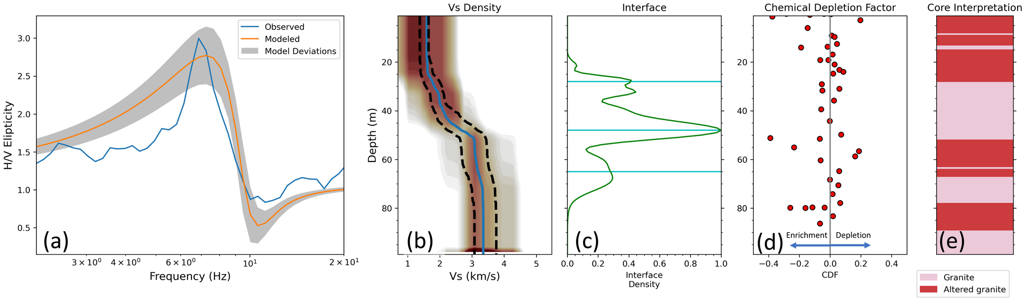
Figure 6Bayesian inversion result of the HVSR curve from the data points closest to the borehole location: (a) observed and modelled HVSR curve; (b) 1D Vs probability density from all the inversion chains and the mean Vs profile, where the blue line is the mean model and the dashed black lines are the uncertainty of the models; (c) interface probability function; (d) CDF from borehole samples; and (e) interpretation from the borehole core.
Since we utilize Voronoi cells in the model parameterization, the Bayesian inversion also produces an interface probability model function (Fig. 6c). This function shows the probability of a likely interface between the layers based on the models produced from all the inversion chains. The interface probability offers four possible interfaces in our data around 15, 28, 48, and 60 m in depth. We also present the calculated CDF in Fig. 6d. The CDF values in the near-surface (< 20 m) show neither a trend in enrichment nor a depletion of the rock samples. Instead, we observe relatively scattered CDF values around zero. We also observe a similar scattering trend around 50–60 m depth and 80 m depth.
5.3 S-wave velocity–depth profile
We compiled the resulting 1D Vs model and interpolated it to create a volumetric cube of Vs value. A series of depth slices from 10–50 m depth is presented in Fig. 7, where we can see a similar NE–SW feature as in Fig. 5. This feature can be observed from 10 m depth and becomes stronger at 20 m. At smaller depths, the velocity is relatively low (< 1.50 km s−1), except around the previously mentioned NE–SW features, with the lowest velocity of around 1.00 km s−1. These low-velocity features remain until 30 m depth (Fig. 7c) where the high velocity starts to take over the low-velocity values around the area. Then, at 40 and 50 m depth, the remaining low-velocity area is located northwest of the borehole.
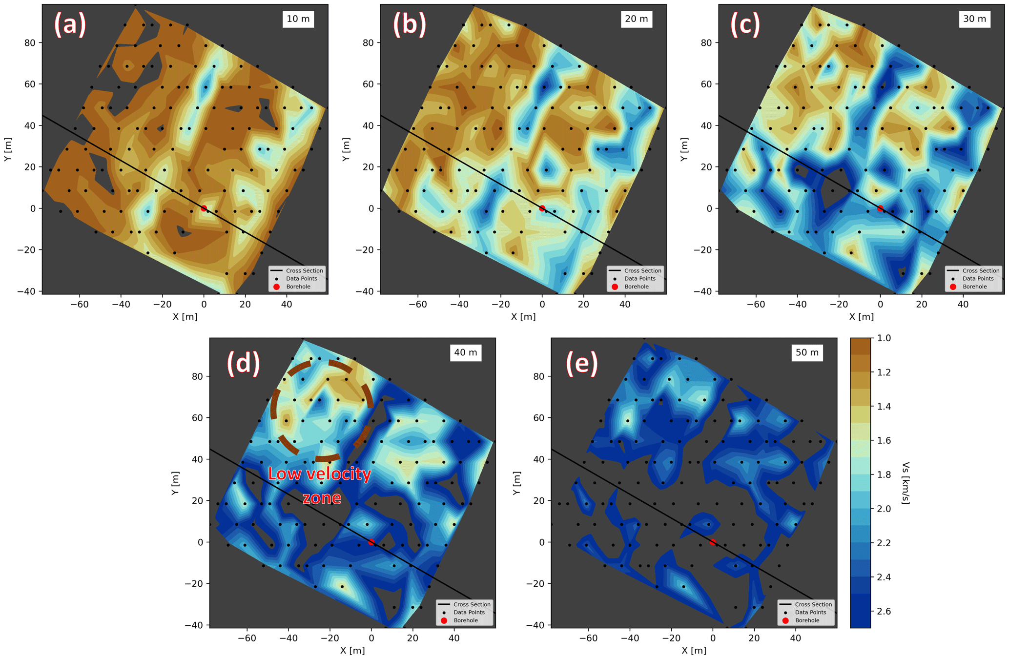
Figure 7Depth slice of the pseudo-3D Vs model produced from the inversion of HVSR curves. From panels (a) to (e) are depth slices with steps of 10 m from the surface. The black dots are the geophone locations, and the black line represents a NW–SE cross-section that goes through the borehole location denoted by the red dot. Greyed-out areas were not covered by the geophone location or have high uncertainty and thus were not resolved.
We also plot a horizontal depth slice of 28 m depth or 693 m above sea level (m a.s.l.) (Fig. 8a) following the end of the altered granite layer interpreted in the borehole core interpretation (Fig. 6e), and, to further investigate the interesting NE–SW features, we also create a vertical slice of our data perpendicular to the NE–SW features and going through the borehole location (Fig. 8b). The vertical slice shows varying Vs between 1.0–3.0 km s−1. Horizontally, we do not see so many variations, except in the western part of the profile, where we can see a relatively lower-velocity layer right before the slope. Vertically, we can divide the profile into three main Vs layers. The first section is the layer with Vs < 1.40 km s−1 which covers down to 15 m in depth. This section is relatively parallel to the surface topography. Then, we have the section with Vs between 1.40 and 2.40 km s−1 which covers a depth between 15 and 30 m and shows more horizontal variations compared to its overlying layer. Finally, the section with Vs > 2.40 km s−1 starts around 30 m in depth near the dashed-line reference in Fig. 8b.
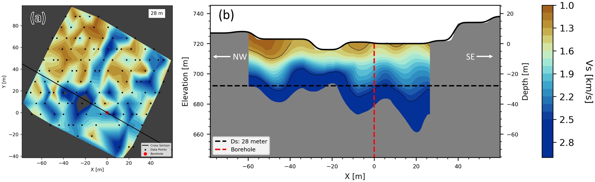
Figure 8Vs model of the study area. (a) Horizontal depth slice at 28 m depth, where the red dot is the borehole, black dots are the station locations, and the solid black line is the cross-section line. (b) Vertical slice from the cross-section line in panel (a). The dashed black line in panel (b) represents the selected 28 m depth line, the dashed red line represents the borehole location, and solid black lines are the 1.30 and 2.50 km s−1 Vs contour lines. The depth axis in panel (b) is relative to borehole elevation (720 m elevation). Panels (a) and (b) use the same colour bar presented on the right.
In addition to the vertical slice across the borehole, we present a vertical section north of the borehole location (Fig. 9). Similar to the profile in Fig. 8b, the Vs value in this profile also ranges between 1.0 and 3.0 km s−1. However, instead of the relatively parallel homogenous horizontal variations in Fig. 8b, in this profile, we can see an interesting near-vertical structure of high velocity ca. 10 m below the surface (Fig. 9b).
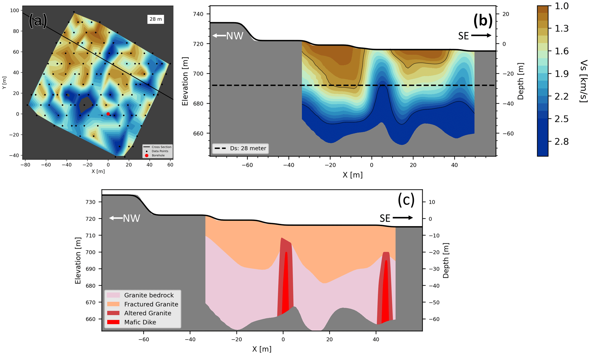
Figure 9Vs model of the study area: (a) horizontal depth slice at 28 m depth, (b) vertical slice from the cross-section line in panel (a), and (c) conceptual model of the cross-section in panel (b). The red dot in panel (a) is the borehole location, and the inverted triangles are the geophone locations. The dashed black line in panel (b) represents the selected 28 m depth line.
Using the HVSR method combined with the hierarchical Bayesian MCMC inversion approach, we managed to image the 3D Vs velocity structure at the arid study site of Pan de Azúcar. We interpret and discuss possible weathering zone structures in the study area using the velocity model. In summary, four main structures in the study area were found: granite bedrock, fractured granite, basaltic intrusion, and hydrothermally altered granite. In addition to the identified structures, we also discuss different controlling processes that could explain the dynamics and formation of the weathering structure in the study area, including the effects of topography. Finally, we compare the structure in Pan de Azúcar to the other EarthShape sites in different climate conditions.
6.1 Granite bedrock
Various Vs values have been used to delineate the upper boundary of physically and chemically unweathered intact granite bedrock formation. Previous studies conducted in similar granitic environments have suggested that a Vs value of 2.0 km s−1 is an appropriate threshold between the granite bedrock and the overlying layer (Liu et al., 2022; Handoyo et al., 2022). Within the context of the EarthShape project, another geophysical investigation conducted at a site with a Mediterranean climate (La Campana National Park; see location in Fig. 1a) has indicated that we can utilize a Vs value of 2.3 km s−1 to identify the upper limit of the bedrock layer (Trichandi et al., 2023). At a site with a semi-arid climate (Santa Gracia National Park; see location in Fig. 1a), another study revealed that a Vs value of 2.5 km s−1 is appropriate for defining the upper boundary of the bedrock interface (Trichandi et al., 2022). We can attribute the selection of different Vs values to determine the bedrock's upper limit either to variation in lithological composition or to the impact of distinct climatic conditions. Nevertheless, given the similarity in climate, we opted to employ a Vs value of 2.5 km s−1 to establish the upper boundary of the bedrock in our study area.
Based on the Vs value across the area in Fig. 7, we can see that the 2.5 km s−1 Vs value started at different depth ranges. In Fig. 7a and b, we can see that, even at shallow depths of 10 and 20 m, Vs is already at 2.5 km s−1. However, we believe that the NE–SE-trending high-Vs zones in the middle of the study area are related to dikes of mafic composition, which we will discuss in Sect. 6.3. Therefore, we believe that the physically intact bedrock starts from 30 m depth at the shallowest, as shown by the high Vs value in the southwestern part of the area shown in Fig. 7c. This high Vs value then becomes more prominent in the 40 and 50 m depth slice (Fig. 7d and e), where we can see that the high Vs value spreads in the northeast direction. Based on this three-dimensional observation, we can already see that, instead of a uniform bedrock depth, as shown in Fig. 8b, the top-of -bedrock depth is more variable in different directions. An intact bedrock depth between 30 to 50 m depth agrees with other previous studies that found intact bedrock depth in an arid and semi-arid area to be between 30 to 70 m depth (Stierman and Healy, 1984; Vázquez et al., 2016; Trichandi et al., 2022).
6.2 Fractured granite
The presence of fractures in the bedrock leads to a systematic decrease in the Vs values. Previous studies have shown that Vs values between 1.3–1.4 km s−1 can be used to identify the top of the fractured bedrock layer (Trichandi et al., 2022, 2023). Based on the horizontal depth slice of the Vs model (Fig. 7), we can already find Vs > 1.3 km s−1 even at 10 m depth (Fig. 7a), even when we exclude the NE–SW high-velocity features.
The low-velocity areas of Vs < 1.3 km s−1 can be explained by several lithologies, including saprolite, colluvial deposits, or highly fractured granite. Saprolite layers from granitic rocks will typically show a much lower Vs value (< 1.0 km s−1) (Trichandi et al., 2022, 2023). Data provided by the borehole also show no indication of a saprolite layer. For colluvial deposits, field observations did observe the existence of a colluvial valley between the two hills, but the extent of this valley fill was not further investigated. Since colluvial valleys will usually show lower Vs values (< 1.0 km s−1) (Handoyo et al., 2022), we opted to attribute this unit to granite rocks with a significantly higher number of fractures within. However, it is also possible that the thickness of this colluvial valley is well below the vertical resolution of our HVSR method; therefore we do not observe its low Vs signature.
The vertical extent of the identified fractured bedrock layer seems to vary significantly across the area: while, on the west of the borehole, Vs values larger than 2 km s−1 are reached at depths shallower than 20 m (blueish zones in Fig. 7c), in the northern part of the area, Vs values lower than 1.3 km s−1 are observed down to 40 m depth (brownish colours in Fig. 7d). This variation across the study area showcases the importance of 3D mapping in weathering front studies, as it is easy to conclude a relatively uniform thickness of the fractured granite layer if we only consider a 2D profile across the borehole (Fig. 8b).
Several processes can explain the fracturing of bedrock in our study area. Firstly, we can hypothesize that the fractures were inherently formed during the cooling process of the plutonic rocks (Ellis and Blenkinsop, 2019). Should this be the case, fractured bedrock in our study area was likely to date back to the emplacement of the Cerros del Vetado, which took place ca. 250–205 Ma. This emplacement likely happened in a depth range of 4–7 km (as per most geobarometry studies of plutonic rocks of the coastal cordillera and precordillera of northern Chile, e.g., Dallmeyer et al., 1996; Dahlström et al., 2022). Another possible explanation for the formation of this fractured granite layer is the process of lithostatic decompression, occurring at shallow depths due to the subduction-induced uplift and erosion of the entire coastal region. Considering that current denudation rates from cosmogenic nuclides are only 7.1 t m−2 yr−1 which corresponds to about 2.7 m Ma−1, the fracturing would have taken place within the past several million years.
6.3 Mafic dikes
The Vs model consistently shows two NE–SW-oriented zones of relatively higher Vs visible from 10 to 50 m depth (Fig. 7). This feature is observed in multiple station locations and shows systematically high Vs values. We interpret these features to be related to the Early Cretaceous NE–SW mafic dikes, which crop out around the study area and intrude on the Triassic Cerros del Vetado pluton (Fig. 1b, d, and e). This hypothesis can explain the higher Vs values as the gabbro and diorite values are higher than granite (e.g., Christensen, 1996). The quasi-linear distribution of outcrops of these dikes in the study area (even when crossing small ridges; see Fig. 1b) suggests that they have high-angle dips, consistent with the vertical shape of high-Vs zones (Fig. 9b).
Hypothetically, we can assume that the intrusion of mafic dikes could be the feature which creates the fractured granite unit. However, it is unlikely (and difficult to prove) that the current fractured granite layer was already present when the dikes emplaced (130 Ma) and that the fractured granite layer has been there over such a long time. According to thermochronological studies in the coastal cordillera of northern Chile (e.g., Juez-Larré et al., 2010; Rodríguez et al., 2018), there were at least two significant exhumation events during the Cretaceous and the Eocene. If there was a shallow fractured granite layer during the emplacement of dikes ca. 130 Ma, it was likely eroded after some of those exhumation events.
Based on the Vs model in Fig. 9b, we create a conceptual lithology model in our cross-section where the dike feature is prominent (Fig. 9c). From the bottom, we have the granite bedrock which was intruded by two mafic dikes. Then, from ca. 30 m depth to the surface, we have an overlying altered and fractured granite. The mafic dikes in our deployment area also do not seem to intrude up to the surface, as we did not find any exposed dike in the middle of the profile during the data acquisition. This is also supported by the high Vs value that does not reach to the surface. Another possible explanation as to why we did not find surface manifestation of the dike could be because of the colluvial fill which covers the middle part of our survey area. Nevertheless, based on this result and findings, we demonstrated the capability of the HVSR method to identify a higher Vs structure in the subsurface even with minimal prior information.
6.4 Altered granite
Chronologically, the Cerros del Vetado pluton emplacement took place 250–205 Ma and likely in a depth range of 4–7 km (as per most geobarometry studies of plutonic rocks of the coastal cordillera and precordillera of northern Chile, e.g., Dallmeyer et al., 1996; Dahlström et al., 2022). Then, the Las Ánimas pluton emplacement took place 160–150 Ma. This later emplacement might have induced hydrothermal alteration in the Cerros del Vetado pluton unit, as identified in the borehole. However, the emplacement of mafic dikes into the Cerros del Vetado pluton granites can also carry heat and possible fluids to enable hydrothermal alteration. The mafic dikes intruded the Cerros del Vetado pluton ca. 130 Ma (i.e., almost 100 Ma after Cerros del Vetado emplacement).
Cores from the borehole shown in Fig. 4a and c show an example of the identified altered granite unit in our borehole location. The altered granite exhibits a relatively reddish colour compared to a relatively intact granite bedrock shown in Fig. 4b, which indicates oxidation of iron minerals. These altered granite units can also be identified by the scattering of the CDF values shown in Fig. 6d. The identified altered granite units also appear to weaken the granite rock as shown in Fig. 4a and c. Weakening of the granite rock in the hydrothermally altered zone is likely due to the formation of secondary mineral which can also trigger micro-fracturing even at depth (Hampl et al., 2023). This weakening of the granite rock will then negatively affect the Vs value.
Since the hydrothermal alteration of the granite rock negatively affects the Vs value, one can also try to interpret the low Vs near the surface across the study area to a hydrothermally altered granite layer. While we lack the information to prove otherwise, we hypothesize that the altered granite in our study area can only be found in close proximity to the possible mafic dike structures. These mafic dike structures provide the heat and fluids to alter the intruded granite rocks around them. However, we also cannot eliminate the possibility of an interconnected fracture network which allows heat and fluid to be transported and enables hydrothermal alteration further away from the mafic dike structures.
6.5 Controlling aspects of weathering structure
Based on the lithology identified in the study area, we summarized several significant controlling aspects that can affect the weathering structure. The first important aspect which could induce a particular weathering structure is the existence of fractures. Previous studies have shown the importance of fractures in facilitating weathering processes (Trichandi et al., 2022; Brantley et al., 2017; Lodes et al., 2023). These fractures can either be formed due to weathering or tectonic processes. The Pan de Azúcar study site is located in a very dry area which limits the chemical weathering process triggered by precipitation. The absence of chemical weathering is also supported by the CDF values shown in Fig. 6d where we observe no clear trend in Nb element enrichment. This is also evident as there is no saprolite layer found in the borehole. Despite the absence of a chemical weathering process, we still observe a reduced seismic velocity which can be attributed to the fractured granite layer. Therefore, we hypothesize that the formation of the fractured granite layer in our study area is due to tectonic stress or lithostatic decompression instead of a chemical weathering process.
The absence of water and vegetation cover in the Pan de Azúcar study sites presents a unique opportunity to study fractured bedrock that precedes weathering processes. The fractures formed in the bedrock, when connected, can act as pathways for fluid or other weathering agents, triggering subsurface chemical weathering of the fractured bedrock. However, since our study site in Pan de Azúcar has no precipitation and vegetation cover, the observed fractured bedrock is likely to be isolated from other weathering processes. This observation is highly unlikely to be found in most locations on Earth with precipitation or vegetation cover which enables physical, chemical, or biological weathering processes.
In addition to the availability of fractures due to preconditioning of the bedrock, the existence of geological structures also plays a significant role in shaping the weathering structure at our study site. A previous study at the Santa Gracia EarthShape site shows how a possible fault could play an important role by allowing deeper weathering and providing fluid infiltration pathways (Trichandi et al., 2022). In Pan de Azúcar, the younger mafic dike intrusion could trigger fracturing, enabling hydrothermal alteration of the surrounding rocks. These findings emphasize the importance of looking at weathering structure not only as a 1D top-down interaction but also as a 3D interplay with the surrounding geological features.
Finally, climate effects in forms of precipitation also highly affect the weathering structure, especially in the near-surface. While our study area shows exposed fractured granite to the surface, the almost absent precipitation restricts the surface's weathering process, which in return changes the fractured bedrock into saprolite. While it is yet to be seen whether fog cover coming in from the Pacific Ocean can affect the weathering structure, our Vs model indicates the absence of saprolite as we do not encounter a very low Vs value (typically below 0.8 km s−1 for saprolite). The absence of the saprolite layer is also supported by the lack of a significant trend in enrichment or depletion in the near-surface as shown by the CDF values in Fig. 6d.
6.6 Weathering depth and climate gradient
We compare the findings from different seismic investigations of the weathering zone across the Chilean climate gradient in Fig. 10. In Fig. 10a, we can see a deepening trend in the average bedrock depth with increased precipitation. Our study using the HVSR method in Pan de Azúcar reveals an average bedrock depth of around 30 m depth. Similarly, in the semi-arid climate of Santa Gracia, evidence from a borehole (Krone et al., 2021) and seismic imaging revealed a weathering front that reaches down to around 30 m in depth (Trichandi et al., 2022). If we observe only these two sites, we can hypothesize either that increasing precipitation has no effect on the bedrock depth or that the increase in precipitation between the arid climate in Pan de Azúcar and the semi-arid climate in Santa Gracia is not significant enough to affect the bedrock depth. However, seismic investigation using the HVSR method in the Mediterranean climate of La Campana (Trichandi et al., 2023) shows a relatively deep average bedrock depth (∼ 60 m depth) compared to the arid and semi-arid sites. When we include this finding, we can see the trend in weathering front deepening with increased precipitation as we go from lower to higher precipitation. This observation confirms that when we have a changing climate, the increase in precipitation can deepen the weathering front. However, there is likely to be a certain threshold to be passed for the increase in precipitation to significantly affect the bedrock depth.
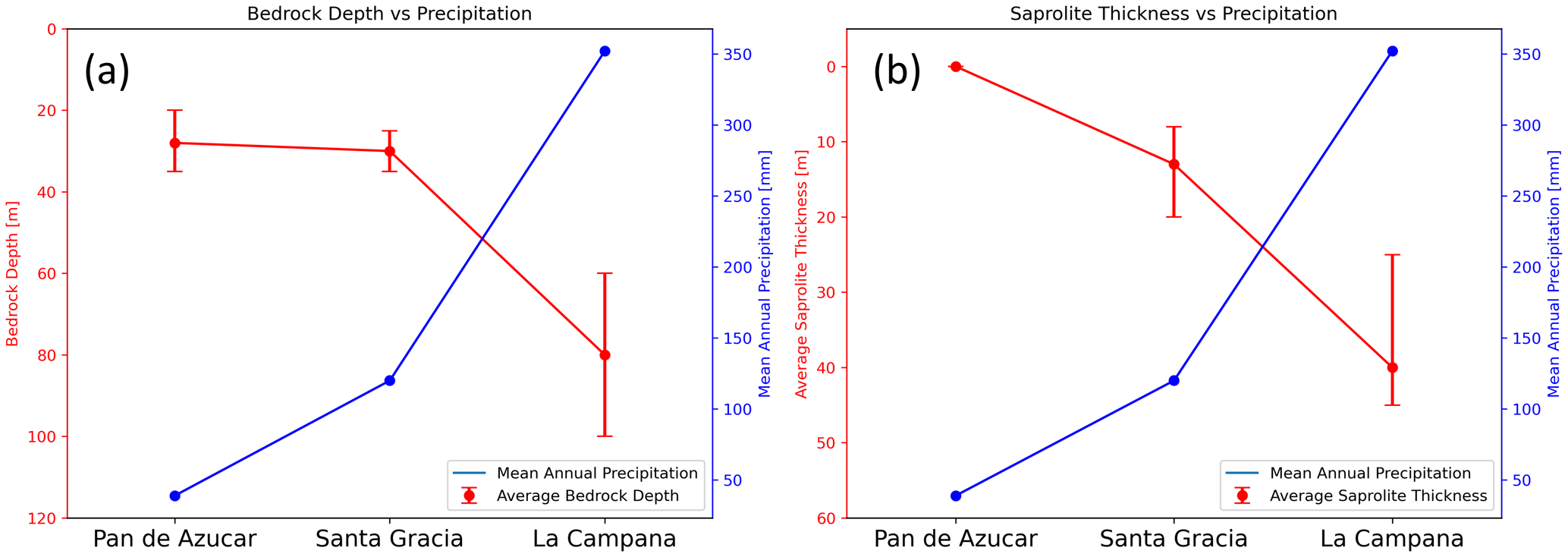
Figure 10Comparison of the precipitation to (a) bedrock depth and (b) saprolite thickness in different EarthShape sites across the Chilean climate gradient. Red lines are (a) the average bedrock depth and (b) the saprolite thickness (Trichandi et al., 2022, 2023). Error bars show the maximum and minimum values. Blue lines are the mean annual precipitation from the different sites (Werner et al., 2018).
We also compare the effect of increased precipitation to the saprolite thickness (Fig. 10b). In the arid climate of Pan de Azúcar, there is a saprolite layer due to the absence of the required weathering agents to transform (fractured) bedrock into saprolite. Unlike their effect on the bedrock depth, precipitation changes between the arid and semi-arid climate of Santa Gracia seem to affect the saprolite thickness more significantly, as we observe 13 m thick saprolite on average across the seismic profile in Santa Gracia (Trichandi et al., 2022). This shows that even when both sites have similar depth extent of the fractured bedrock as the preconditioning to enable weathering processes, the climate condition in Pan de Azúcar does not satisfy the condition to trigger extensive weathering of the fractured bedrock to saprolite. The thickening of the saprolite layer due to increase in precipitation is even more pronounced when we compare the saprolite thickness in Santa Gracia to the Mediterranean climate of La Campana, where we observed a significantly thicker saprolite layer up to 55 m thick (Trichandi et al., 2023).
This paper presents a unique case of bedrock which has been pre-conditioned (fractured) but has yet to be weathered. The depth of the bedrock does not deepen significantly when we go into the semi-arid climate. However, the increase in precipitation enables saprolite production, as precipitation provides the required weathering agent to reach the subsurface through the available inherent fractures. Therefore, in addition to the depth of the weathering front, it is important to discuss the saprolite thickness when studying the effects of changing climate to the weathering zone structure, as it correlates with the weathering intensity of the study area.
The presented study showcases the importance of imaging the weathering zone, not only in 2D but also from a 3D point of view. Applying the HVSR method with the Bayesian inversion scheme provides a straightforward technique for 3D imaging of the weathering structure. The passive seismic nature of the HVSR method also enables data acquisition where usage of an active seismic source is restricted or even prohibited. The resulting 3D model also revealed dike features which we would not find if we only did 2D imaging of the subsurface.
Based on the Vs model, we identified fractured and altered granite in Pan de Azúcar to reach a depth of 30–40 m. There is no Vs signature of a saprolite layer that is indeed absent in Pan de Azúcar due to the arid climate, as also shown by the CDF values of the borehole core. Mafic dike structures, which can be the source of hydrothermal alteration, were identified in the study area. Comparing the results of Pan de Azúcar (arid climate) with the Santa Gracia (semi-arid) and La Campana (Mediterranean) EarthShape sites, we interpret that the depth and structure of the weathering zone are a result of the complex interplay between fluid infiltration, the presence of interconnected pathways allowing fluid to migrate to great depth, and the mineralogy of the bedrock before being exposed to surficial weathering. The imaged structure of the subsurface in Pan de Azúcar is unique in the sense that it shows a rock preconditioned for weathering but one that has never experienced any extensive weathering given the absence of precipitation.
This study also further emphasizes the vital role of geophysical methods in imaging the weathering zone. This work shows that the employed seismic method helped differentiate geological features with distinctive weathering conditions (e.g., mafic dikes and the granites) that can be further investigated using a method with high resolution (e.g., borehole). This study also shows the importance of imaging the weathering zone in 3D, as the structures of the weathering zone can exhibit significant variations in the horizontal direction.
The data that support the findings will be available in the GFZ data repository following an embargo to allow for doctoral publication of research findings.
RT, KB, and CMK planned the campaign. RT and BH performed the measurements. RT, KB, and TR analysed the data. RT wrote the draft. KB, TR, BH, JAV, FvB, and CMK reviewed and edited the paper.
The contact author has declared that none of the authors has any competing interests.
Publisher’s note: Copernicus Publications remains neutral with regard to jurisdictional claims made in the text, published maps, institutional affiliations, or any other geographical representation in this paper. While Copernicus Publications makes every effort to include appropriate place names, the final responsibility lies with the authors.
This article is part of the special issue “Earth surface shaping by biota (Esurf/BG/SOIL/ESD/ESSD inter-journal SI)”. It is not associated with a conference.
We acknowledge support from the German Science Foundation (DFG) priority research programme SPP-1803 “EarthShape: Earth surface shaping by biota”. Instruments for data acquisition were supported by the Geophysical Instrumental Pool Potsdam – GIPP (grant no. GIPP-201924). This work was also supported by EarthShape Coordination. The authors are very grateful to Kirstin Übernickel for her support in planning and performing the drilling campaign and downhole logging. We are also grateful to Brady Flinchum and the anonymous reviewer who gave invaluable comments and suggestions.
This research has been supported by the Deutsche Forschungsgemeinschaft (grant nos. KR 2073/5-1, EH 329/17-2, and BL 562/20-1).
The article processing charges for this open-access publication were covered by the Helmholtz Centre Potsdam – GFZ German Research Centre for Geosciences.
This paper was edited by Tom Coulthard and reviewed by Brady Flinchum and one anonymous referee.
Acevedo, J.: Análisis petrológico/mineralógico y estructural del Plutón Cerros del Vetado, comuna de Chañaral, región de Atacama, Universidad de Atacama, https://repositorioacademico.uda.cl/bitstream/handle/20.500.12740/16421/Bib 29.439.pdf?sequence=1&isAllowed=y (last access: 5 May 2024), 2022.
Arai, H. and Tokimatsu, K.: S-Wave Velocity Profiling by Inversion of Microtremor H/V Spectrum, B. Seismol. Soc. Am., 94, 53–63, https://doi.org/10.1785/0120030028, 2004.
Befus, K. M. M., Sheehan, A. F. F., Leopold, M., Anderson, S. P. P., and Anderson, R. S. S.: Seismic Constraints on Critical Zone Architecture, Boulder Creek Watershed, Front Range, Colorado, Vadose Zone J., 10, 915, https://doi.org/10.2136/vzj2010.0108, 2011.
Berg, K. and Baumann, A.: Plutonic and metasedimentary rocks from the Coastal Range of northern Chile: RbSr and UPb isotopic systematics, Earth Planet. Sc. Lett., 75, 101–115, https://doi.org/10.1016/0012-821X(85)90093-7, 1985.
Bodin, T.: Transdimensional Approaches to Geophysical Inverse Problems, PhD thesis, 243 pp., https://doi.org/10.1021/jo00151a027, 2010.
Bodin, T., Sambridge, M., Tkalćić, H., Arroucau, P., Gallagher, K., and Rawlinson, N.: Transdimensional inversion of receiver functions and surface wave dispersion, J. Geophys. Res.-Sol. Ea., 117, 1–24, https://doi.org/10.1029/2011JB008560, 2012.
Brantley, S. L., Lebedeva, M. I., Balashov, V. N., Singha, K., Sullivan, P. L., and Stinchcomb, G.: Toward a conceptual model relating chemical reaction fronts to water flow paths in hills, Geomorphology, 277, 100–117, https://doi.org/10.1016/j.geomorph.2016.09.027, 2017.
Brocher, T. M.: Empirical relations between elastic wavespeeds and density in the Earth's crust, B. Seismol. Soc. Am., 95, 2081–2092, https://doi.org/10.1785/0120050077, 2005.
Christensen, N. I.: Poisson's ratio and crustal seismology, J. Geophys. Res.-Sol. Ea., 101, 3139–3156, https://doi.org/10.1029/95JB03446, 1996.
Cipta, A., Cummins, P., Dettmer, J., Saygin, E., Irsyam, M., Rudyanto, A., and Murjaya, J.: Seismic velocity structure of the Jakarta Basin, Indonesia, using trans-dimensional Bayesian inversion of horizontal-to-vertical spectral ratios, Geophys. J. Int., 215, 431–449, https://doi.org/10.1093/gji/ggy289, 2018.
Cox, B. R., Cheng, T., Vantassel, J. P., and Manuel, L.: A statistical representation and frequency-domain window-rejection algorithm for single-station HVSR measurements, Geophys. J. Int., 221, 2170–2183, https://doi.org/10.1093/GJI/GGAA119, 2021.
Dahlström, S. I. R., Cooper, F. J., Blundy, J., Tapster, S., Yáñez, J. C., and Evenstar, L. A.: Pluton Exhumation in the Precordillera of Northern Chile (17.8°–24.2° S): Implications for the Formation, Enrichment, and Preservation of Porphyry Copper Deposits, Econ. Geol., 117, 1043–1071, https://doi.org/10.5382/econgeo.4912, 2022.
Dal Bo, I., Klotzsche, A., Schaller, M., Ehlers, T. A., Kaufmann, M. S., Fuentes Espoz, J. P., Vereecken, H., and van der Kruk, J.: Geophysical imaging of regolith in landscapes along a climate and vegetation gradient in the Chilean coastal cordillera, Catena, 180, 146–159, https://doi.org/10.1016/j.catena.2019.04.023, 2019.
Dallmeyer, R. D., Brown, M., Grocott, J., Taylor, G. K., and Treloar, P. J.: Mesozoic Magmatic and Tectonic Events within the Andean Plate Boundary Zone, 26°–27°30′ S, North Chile: Constraints from 40 Ar 39 Ar Mineral Ages, J. Geol., 104, 19–40, https://doi.org/10.1086/629799, 1996.
Ellis, J. F. and Blenkinsop, T.: Analogue modelling of fracturing in cooling plutonic bodies, Tectonophysics, 766, 14–19, https://doi.org/10.1016/j.tecto.2019.05.019, 2019.
Fäh, D., Kind, F., and Giardini, D.: Inversion of local S-wave velocity structures from average ratios, and their use for the estimation of site-effects, J. Seismol., 7, 449–467, https://doi.org/10.1023/B:JOSE.0000005712.86058.42, 2003.
Flinchum, B. A., Steven Holbrook, W., Rempe, D., Moon, S., Riebe, C. S., Carr, B. J., Hayes, J. L., Clair, J. S., and Peters, M. P.: Critical zone structure under a granite ridge inferred from drilling and three-dimensional seismic refraction data, J. Geophys. Res.-Earth, 123, 1317–1343, https://doi.org/10.1029/2017JF004280, 2018.
Godoy, E. and Lara, L.: Hojas Chañaral y Diego de Almagro, Región de Atacama, Servicio Nacional de Geología y Minería, Mapas Geológicos No. 5–6, 1 mapa escala 1:100.000, Santiago, https://tiendadigital.sernageomin.cl/en/basic-geology/887-1998hojas-chanaral-y-diego-de-almagro-region-de-atacama-escala-1-100000.html (last access: 5 May 2024), 1998.
Hampl, F. J., Schiperski, F., Schwerdhelm, C., Stroncik, N., Bryce, C., von Blanckenburg, F., and Neumann, T.: Feedbacks between the formation of secondary minerals and the infiltration of fluids into the regolith of granitic rocks in different climatic zones (Chilean Coastal Cordillera), Earth Surf. Dynam., 11, 511–528, https://doi.org/10.5194/esurf-11-511-2023, 2023.
Handoyo, H., Defelipe, I., Martín-Banda, R., García-Mayordomo, J., Martí, D., Martínez-Díaz, J. J., Insua-Arévalo, J. M., Teixidó, T., Alcalde, J., Palomeras, I., and Carbonell, R.: Characterization of the shallow subsurface structure across the Carrascoy Fault System (SE Iberian Peninsula) using P-wave tomography and Multichannel Analysis of Surface Waves, Geol. Acta, 20, 1–19, https://doi.org/10.1344/GeologicaActa2022.20.9, 2022.
Hobiger, M., Cornou, C., Wathelet, M., Di Giulio, G., Knapmeyer-Endrun, B., Renalier, F., Bard, P. Y., Savvaidis, A., Hailemikael, S., Le Bihan, N., Ohrnberger, M., and Theodoulidis, N.: Ground structure imaging by inversions of Rayleigh wave ellipticity: Sensitivity analysis and application to European strong-motion sites, Geophys. J. Int., 192, 207–229, https://doi.org/10.1093/gji/ggs005, 2013.
Holbrook, W. S., Riebe, C. S., Elwaseif, M., Hayes, J. L., Basler-Reeder, K., Harry, D. L., Malazian, A., Dosseto, A., Hartsough, P. C., and Hopmans, J. W.: Geophysical constraints on deep weathering and water storage potential in the Southern Sierra Critical Zone Observatory, Earth Surf. Proc. Land., 39, 366–380, https://doi.org/10.1002/esp.3502, 2014.
Jara, J. J., Barra, F., Reich, M., Morata, D., Leisen, M., and Romero, R.: Geochronology and petrogenesis of intrusive rocks in the Coastal Cordillera of northern Chile: Insights from zircon U–Pb dating and trace element geochemistry, Gondwana Res., 93, 48–72, https://doi.org/10.1016/j.gr.2021.01.007, 2021.
Juez-Larré, J., Kukowski, N., Dunai, T. J., Hartley, A. J., and Andriessen, P. A. M.: Thermal and exhumation history of the Coastal Cordillera arc of northern Chile revealed by thermochronological dating, Tectonophysics, 495, 48–66, https://doi.org/10.1016/j.tecto.2010.06.018, 2010.
Karger, D. N., Conrad, O., Böhner, J., Kawohl, T., Kreft, H., Soria-Auza, R. W., Zimmermann, N. E., Linder, H. P., and Kessler, M.: Climatologies at high resolution for the earth's land surface areas, Sci. Data, 4, 1–20, https://doi.org/10.1038/sdata.2017.122, 2017.
Koesuma, S., Ridwan, M., Nugraha, A. D., Widiyantoro, S., and Fukuda, Y.: Preliminary estimation of engineering bedrock depths from microtremor array measurements in Solo, Central Java, Indonesia, J. Math. Fundam. Sci., 49, 306–320, https://doi.org/10.5614/j.math.fund.sci.2017.49.3.8, 2017.
Krone, L. V, Hampl, F. J., Schwerdhelm, C., Bryce, C., Ganzert, L., Kitte, A., Übernickel, K., Dielforder, A., Aldaz, S., Oses-Pedraza, R., Perez, J. P. H., Sanchez-Alfaro, P., Wagner, D., Weckmann, U., and von Blanckenburg, F.: Deep weathering in the semi-arid Coastal Cordillera, Chile, Sci. Rep., 11, 1–15, https://doi.org/10.1038/s41598-021-90267-7, 2021.
Lehnert, L. W., Thies, B., Trachte, K., Achilles, S., Osses, P., Baumann, K., Schmidt, J., Samolov, E., Jung, P., Leinweber, P., Karsten, U., Büdel, B., and Bendix, J.: A case study on fog/low stratus occurrence at las lomitas, atacama desert (Chile) as a water source for biological soil crusts, Aerosol Air Qual. Res., 18, 254–269, https://doi.org/10.4209/aaqr.2017.01.0021, 2018.
Liu, X., Zhu, T., and Hayes, J.: Critical Zone Structure by Elastic Full Waveform Inversion of Seismic Refractions in a Sandstone Catchment, Central Pennsylvania, USA, J. Geophys. Res.-Sol. Ea., 127, 1–17, https://doi.org/10.1029/2021JB023321, 2022.
Lodes, E., Scherler, D., van Dongen, R., and Wittmann, H.: The story of a summit nucleus: hillslope boulders and their effect on erosional patterns and landscape morphology in the Chilean Coastal Cordillera, Earth Surf. Dynam., 11, 305–324, https://doi.org/10.5194/esurf-11-305-2023, 2023.
Maghami, S., Sohrabi-Bidar, A., Bignardi, S., Zarean, A., and Kamalian, M.: Extracting the shear wave velocity structure of deep alluviums of “Qom” Basin (Iran) employing HVSR inversion of microtremor recordings, J. Appl. Geophys., 185, 104246, https://doi.org/10.1016/j.jappgeo.2020.104246, 2021.
Mahajan, A. K., Mundepi, A. K., Chauhan, N., Jasrotia, A. S., Rai, N., and Gachhayat, T. K.: Active seismic and passive microtremor HVSR for assessing site effects in Jammu city, NW Himalaya, India – A case study, J. Appl. Geophys., 77, 51–62, https://doi.org/10.1016/j.jappgeo.2011.11.005, 2012.
Maksaev, V., Munizaga, F., and Tassinari, C.: Timing of the magmatism of the paleo-pacific border of Gondwana: U–Pb geochronology of Late Paleozoic to Early Mesozoic igneous rocks of the north Chilean Andes between 20° and 31° S, Andean Geol., 41, 447–506, https://doi.org/10.5027/andgeoV41n3-a01, 2014.
Moon, S. W., Subramaniam, P., Zhang, Y., Vinoth, G., and Ku, T.: Bedrock depth evaluation using microtremor measurement: empirical guidelines at weathered granite formation in Singapore, J. Appl. Geophys., 171, 103866, https://doi.org/10.1016/j.jappgeo.2019.103866, 2019.
Nagamani, D., Sivaram, K., Rao, N. P., and Satyanarayana, H. V. S.: Ambient noise and earthquake HVSR modelling for site characterization in southern mainland, Gujarat, J. Earth Syst. Sci., 129, 195, https://doi.org/10.1007/s12040-020-01443-8, 2020.
Nakamura, Y.: A method for dynamic characteristics estimation of subsurface using microtremor on ground surface, Railw. Tech. Res. Institute, Q. Reports, 30, 25–33, 1989.
Nelson, S. and McBride, J.: Application of HVSR to estimating thickness of laterite weathering profiles in basalt, Earth Surf. Proc. Land., 44, 1365–1376, https://doi.org/10.1002/esp.4580, 2019.
Oeser, R. A. and von Blanckenburg, F.: Do degree and rate of silicate weathering depend on plant productivity?, Biogeosciences, 17, 4883–4917, https://doi.org/10.5194/bg-17-4883-2020, 2020.
Oeser, R. A., Stroncik, N., Moskwa, L. M., Bernhard, N., Schaller, M., Canessa, R., van den Brink, L., Köster, M., Brucker, E., Stock, S., Fuentes, J. P., Godoy, R., Matus, F. J., Oses Pedraza, R., Osses McIntyre, P., Paulino, L., Seguel, O., Bader, M. Y., Boy, J., Dippold, M. A., Ehlers, T. A., Kühn, P., Kuzyakov, Y., Leinweber, P., Scholten, T., Spielvogel, S., Spohn, M., Übernickel, K., Tielbörger, K., Wagner, D., and von Blanckenburg, F.: Chemistry and microbiology of the Critical Zone along a steep climate and vegetation gradient in the Chilean Coastal Cordillera, Catena, 170, 183–203, https://doi.org/10.1016/j.catena.2018.06.002, 2018.
Olona, J., Pulgar, J. A., Fernández-Viejo, G., López-Fernández, C., and González-Cortina, J. M.: Weathering variations in a granitic massif and related geotechnical properties through seismic and electrical resistivity methods, Near Surf. Geophys., 8, 585–599, https://doi.org/10.3997/1873-0604.2010043, 2010.
Parolai, S., Picozzi, M., Richwalski, S. M., and Milkereit, C.: Joint inversion of phase velocity dispersion and ratio curves from seismic noise recordings using a genetic algorithm, considering higher modes, Geophys. Res. Lett., 32, L01303, https://doi.org/10.1029/2004GL021115, 2005.
Pastén, C., Sáez, M., Ruiz, S., Leyton, F., Salomón, J., and Poli, P.: Deep characterization of the Santiago Basin using HVSR and cross-correlation of ambient seismic noise, Eng. Geol., 201, 57–66, https://doi.org/10.1016/j.enggeo.2015.12.021, 2016.
Pilz, M., Parolai, S., Picozzi, M., Wang, R., Leyton, F., Campos, J., and Zschau, J.: Shear wave velocity model of the Santiago de Chile basin derived from ambient noise measurements: A comparison of proxies for seismic site conditions and amplification, Geophys. J. Int., 182, 355–367, https://doi.org/10.1111/j.1365-246X.2010.04613.x, 2010.
Piña-Flores, J., Cárdenas-Soto, M., García-Jerez, A., Seivane, H., Luzón, F., and Sánchez-Sesma, F. J.: Use of peaks and troughs in the horizontal-to-vertical spectral ratio of ambient noise for Rayleigh-wave dispersion curve picking, J. Appl. Geophys., 177, 104024, https://doi.org/10.1016/j.jappgeo.2020.104024, 2020.
Riebe, C. S., Kirchner, J. W., and Finkel, R. C.: Long-term rates of chemical weathering and physical erosion from cosmogenic nuclides and geochemical mass balance, Geochim. Cosmochim. Ac., 67, 4411–4427, https://doi.org/10.1016/S0016-7037(03)00382-X, 2003.
Rodríguez, M. P., Charrier, R., Brichau, S., Carretier, S., Farías, M., Parseval, P., and Ketcham, R. A.: Latitudinal and Longitudinal Patterns of Exhumation in the Andes of North-Central Chile, Tectonics, 37, 2863–2886, https://doi.org/10.1029/2018TC004997, 2018.
Ryberg, T. and Haberland, C.: Bayesian simultaneous inversion for local earthquake hypocentres and 1-D velocity structure using minimum prior knowledge, Geophys. J. Int., 218, 840–854, https://doi.org/10.1093/gji/ggz177, 2019.
Sernageomin: Mapa Geológico de Chile, Servicio Nacional de Geología y Minería Santiago, https://tiendadigital.sernageomin.cl/es/geologia-basica/3209-mapa-geologico-de-chile.html (last access: 5 May 2024), 1982.
SESAME: Guidelines for The Implementation of The H/V Spectral Ratio Technique on Ambient Vibrations-Measurements, Processing and Interpretations, SESAME European Research Project, SESAME Site Eff. Assess. using Ambient Excit., 62 pp., https://sesame.geopsy.org/Delivrables/Del-D23-HV_User_Guidelines.pdf (last access: 5 May 2024), 2004.
Stannard, D., Meyers, J., and Dronfield, T.: Passive seismic horizontal to vertical spectral ratio (HVSR) surveying to help define bedrock depth, structure and layering in shallow coal basins, ASEG Ext. Abstr., 2019, 1–5, https://doi.org/10.1080/22020586.2019.12073175, 2019.
Stierman, D. J. and Healy, J. H.: A study of the depth of weathering and its relationship to the mechanical properties of near-surface rocks in the Mojave Desert, Pure Appl. Geophys., 122, 425–439, https://doi.org/10.1007/BF00874609, 1984.
Trichandi, R., Bauer, K., Ryberg, T., Scherler, D., Bataille, K., and Krawczyk, C. M.: Combined seismic and borehole investigation of the deep granite weathering structure – Santa Gracia Reserve case in Chile, Earth Surf. Proc. Land., 47, 1–15, https://doi.org/10.1002/esp.5457, 2022.
Trichandi, R., Bauer, K., Ryberg, T., Wawerzinek, B., Araya Vargas, J., von Blanckenburg, F., and Krawczyk, C. M.: Shear-wave velocity imaging of weathered granite in La Campana (Chile) from Bayesian inversion of micro-tremor spectral ratios, J. Appl. Geophys., 217, 105191, https://doi.org/10.1016/j.jappgeo.2023.105191, 2023.
Vantassel, J.: hvsrpy, Zenodo [code], https://doi.org/10.5281/zenodo.3666956, 2020.
Vázquez, M., Ramírez, S., Morata, D., Reich, M., Braun, J. J., and Carretier, S.: Regolith production and chemical weathering of granitic rocks in central Chile, Chem. Geol., 446, 87–98, https://doi.org/10.1016/j.chemgeo.2016.09.023, 2016.
Wathelet, M., Chatelain, J. L., Cornou, C., Giulio, G. Di, Guillier, B., Ohrnberger, M., and Savvaidis, A.: Geopsy: A user-friendly open-source tool set for ambient vibration processing, Seismol. Res. Lett., 91, 1878–1889, https://doi.org/10.1785/0220190360, 2020.
Wathelet, M., Jongmans, D., and Ohrnberger, M.: Surface-wave inversion using a direct search algorithm and its application to ambient vibration measurements, Near Surf. Geophys., 2, 211–221, https://doi.org/10.3997/1873-0604.2004018, 2004.
Werner, C., Schmid, M., Ehlers, T. A., Fuentes-Espoz, J. P., Steinkamp, J., Forrest, M., Liakka, J., Maldonado, A., and Hickler, T.: Effect of changing vegetation and precipitation on denudation – Part 1: Predicted vegetation composition and cover over the last 21 thousand years along the Coastal Cordillera of Chile, Earth Surf. Dynam., 6, 829–858, https://doi.org/10.5194/esurf-6-829-2018, 2018.
Xu, R. and Wang, L.: The horizontal-to-vertical spectral ratio and its applications, EURASIP J. Adv. Sig. Pr., 2021, 75, https://doi.org/10.1186/s13634-021-00765-z, 2021.