the Creative Commons Attribution 4.0 License.
the Creative Commons Attribution 4.0 License.
 | 10 Jun 2024
A machine learning approach to the geomorphometric detection of ribbed moraines in Norway
Thomas J. Barnes
Thomas V. Schuler
Simon Filhol
Karianne S. Lilleøren
Machine learning is a powerful yet underutilised tool in geomorphology, commonly used for image-based pattern recognition. Analysing new high-resolution (1–10 m) elevation datasets, we investigate its usefulness for detecting discrete geomorphological features. This study develops a machine-learning-based method for identifying ribbed moraines in digital elevation data and progresses to test its performance versus time-consuming, manual methods. Ribbed moraines share geomorphometric characteristics with other glacial landforms, hence representing a valuable test of our new methodology in terms of differentiating between similar features, and for detecting landforms with similar characteristics. Furthermore, mapping ribbed moraines may provide valuable indications of their origin, a topic of debate within glacial geomorphology. To automatically detect ribbed moraines, we extract simple morphometrics from high-resolution digital elevation model data and mask regions where ribbed moraines are unlikely to form. We then test several machine learning algorithms before examining the best performer (K-means clustering) for three study areas of 15 km2 in Norway. Our results demonstrate a balanced accuracy of 65 %–75 % when validating versus ground-truthing. The performance depends on the availability of high-resolution elevation data in Norway that are needed to resolve the spatial scale of the target (10–100 m). We find the method effective at detecting both fields of ribbed moraines, as well as individual ribbed moraines. We propose pathways for the future implementation of this method on a large scale and for increasing the detail of information gained about detected landforms. In conclusion, we demonstrate K-means clustering as a promising method for detecting ribbed moraines, with great potential to reduce the time needed to produce landform maps.
- Article
(8816 KB) - Full-text XML
- BibTeX
- EndNote


1.1 Geomorphological mapping
Mapping of landforms has traditionally been a manual process, either through direct field observations or manual analysis of remotely sensed data (Smith and Clark, 2005; Verstappen, 2011; Evans, 2012; Sommerkorn, 2020). More recently, semi-automated methods have been developed, where computational analysis of remote sensing data is interpreted by the operator (Guitet et al., 2013), giving rise to subjectivity and human error (Saha et al., 2011; Eisank et al., 2014; Sommerkorn, 2020). Often, the restriction of data availability, quality, and resolution have been the primary limitations leading to the maintenance of traditional approaches, as the resolution of digital elevation models (DEMs) has typically been limited to 30–300 m (Saha et al., 2011; Iwahashi et al., 2018), thus inhibiting the detection of metre-scale features. Additionally, until recently, sub-10 m datasets have been afflicted with patchy coverage (UKEA, 2023), limiting large-scale, high-resolution digital mapping of smaller (sub-data-resolution) landforms.
1.2 Machine learning as a solution
In recent years, automated landform mapping has taken a machine-learning-based pattern recognition approach, starting with a DEM and extracting morphometrics from input data, such as slope, aspect, convexity, and surface texture (Clubb et al., 2019; Eisank et al., 2014; Saha et al., 2011; Iwahashi et al., 2018). Thus far, machine learning approaches focused on large-scale geomorphological feature detection, such as sedimentary basins or terrain classification due to resolution restrictions (Kong et al., 2021; Iwahashi et al., 2018). Yet, the increasing availability of high-resolution (<10 m) datasets (e.g. Kartverket, 2021b; UKEA, 2023) enables individual feature mapping for large areas. Norway has a national high-resolution (0.6–1 m) DEM and orthophotography data coverage (Kartverket, 2021a, c). In conjunction with this, the development of new and more robust machine learning methods, coupled with the effectiveness of older methods with new, high-resolution data (clustering and segmentation; Gentleman and Carey, 2008), suggests that new approaches for small-scale landform detection are now possible.
As machine learning is fast, low on labour intensiveness once set up, and minimises human error (Gentleman and Carey, 2008), it is clear that it may be possible to address prior limitations to landform mapping. However, as high-resolution data availability is a recent development, only few studies, for example, Corr et al. (2022), used a supervised random forest (RF) algorithm to detect supraglacial lakes in Antarctica. Aydda et al. (2020) detected dune forms using three different unsupervised machine learning algorithms, including K-means clustering (KM). Here, we propose combining new, high-resolution data and machine learning to overcome previous limitations in geomorphological mapping.
1.3 Study aims
In this study, we develop a machine learning algorithm to detect specific small-scale geomorphological landforms in high-resolution DEM data, more specifically ribbed moraine. They usually have horizontal extents at a 10–100 m scale and are common in Norway (Dunlop and Clark, 2006; Dunlop et al., 2008; Hättestrand and Kleman, 1999; Finlayson and Bradwell, 2008). Furthermore, they typically form in shallow depressions in inland regions close to the former Fennoscandian ice divide (Sollid and Sorbel, 1994; Sarala, 2006; Fredin et al., 2013; Sommerkorn, 2020; Patton et al., 2016, 2017; Butcher et al., 2021). With this information, we can define potential study regions and a validation dataset. Ribbed moraines are subglacial ridges transverse to the glacial flow direction (Fig. 1) (Dunlop and Clark, 2006) and were documented across Canada and Fennoscandia in the mid-1900s (Hoppe, 1952; Frödin, 1954; Cowan, 1968; Lundqvist, 1969). They also are known to be present near morphologically similar landforms such as drumlins and hummocks, suggesting related formational processes. This spatial relationship raises the prospect of a “bedform continuum” present beneath ice sheets (Aario, 1977; Lundqvist, 1989, 1997; Dunlop and Clark, 2006; Ely et al., 2016; Möller and Dowling, 2018). Furthermore, this spatial relationship allows us to determine whether our approach can differentiate between different landforms with similar morphologies and spatial extents – this is possible through iteration with ribbed-moraine-specific parameters across an area containing “ribbed moraine” and “non-ribbed moraine” landforms. In addition, we note scientific interest in specifically mapping ribbed moraines, the origin of which is still a matter of debate (Möller, 2010; Lindén et al., 2008; Boulton and Clark, 1990; Fisher and Shaw, 1992; Dunlop et al., 2008; Sollid and Sorbel, 1994).
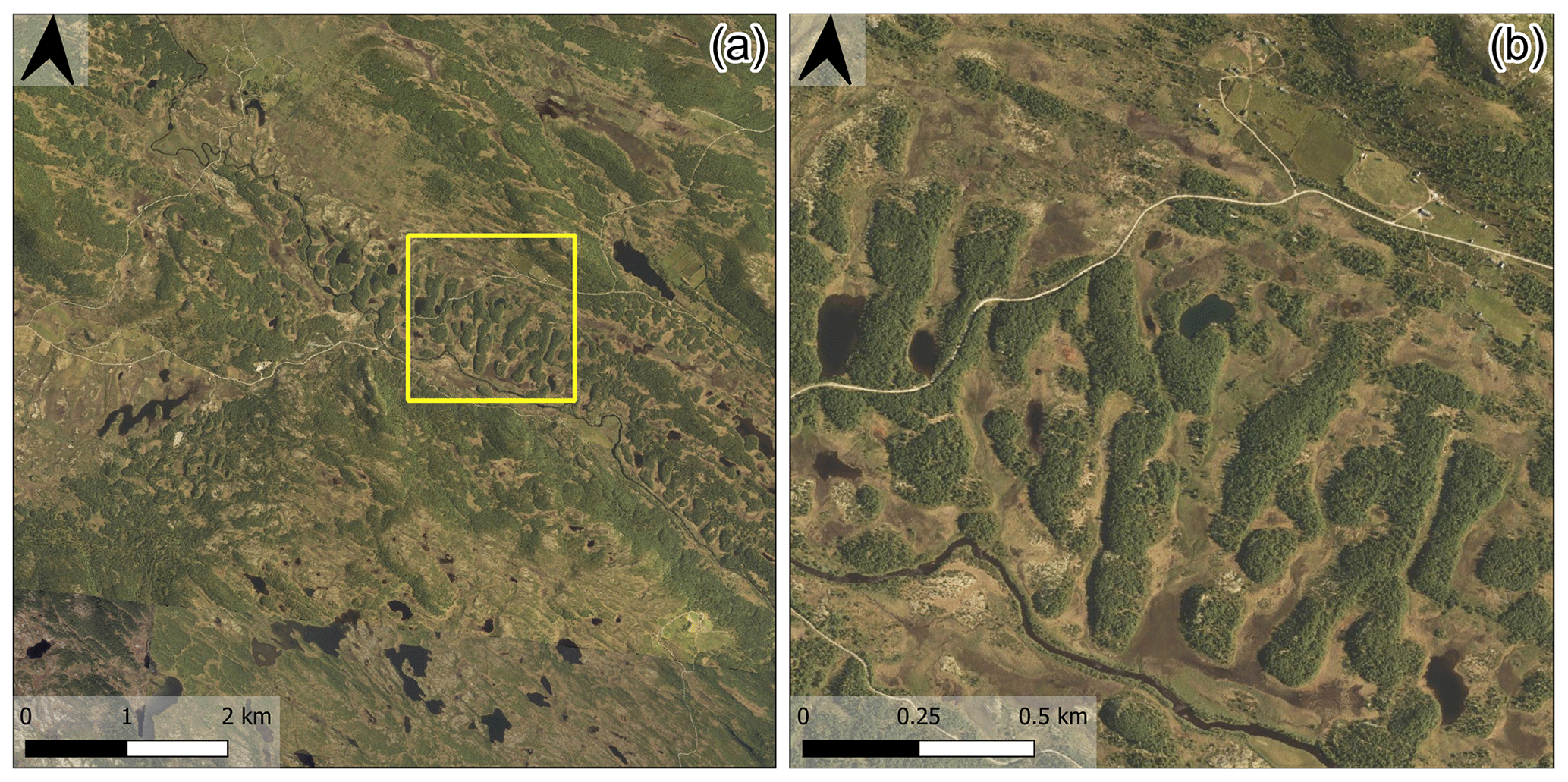
Figure 1Aerial imagery of ribbed moraine at the Vinstre study area site (Fig. 3d), with panel (a) showing a general overview and panel (b) showing a close-up view of ribbed moraine landforms. Ribbed moraines at this site appear to be partially anastomosed and form in a linear track (Dunlop and Clark, 2006). Aerial imagery is from Norwegian national mapping data (Kartverket, 2021a, c).
Here, we develop and test two simple machine learning algorithms, KM and RF (Gentleman and Carey, 2008), applied on new high-resolution datasets to design a computationally efficient, accurate, and transferable method for automatically mapping ribbed moraine (Fig. 1). We define our performance metrics in terms of efficiency, the processing speed of the method; effectiveness, the accuracy of the method; and transferability, how well the method performs in different terrain types on a regional/country-wide scale. We further discuss the potential extensions to detect other landforms such as eskers, drumlins, and megaripples.
2.1 Machine learning
There are several machine learning approaches used previously in geomorphological research that may be useful for automatic feature detection. Many others exist, including U-net, a deep-learning image segmentation method (Ronneberger et al., 2015); however, a main consideration of this study is to improve the time efficiency of landform detection. Despite rapid segmentation once trained, U-net takes large amounts of time to train compared to random forest and K-means clustering (KM). Thus, we identify random forest and KM as two simple and lightweight methods that are used for similar image segmentation problems. The first and simplest approach is unsupervised machine learning (Gentleman and Carey, 2008). Unsupervised machine learning produces a segmented output from input data and does not require training data (a dataset designed to describe what the algorithm should look for). The algorithm identifies clusters based on the similarity of data properties (Gentleman and Carey, 2008). One such method is KM, often used in image segmentation (Burney and Tariq, 2014). Second, supervised machine learning methods such as random forest (RF) require a training dataset consisting of labelled data to provide a true reference for training the algorithm (Gentleman and Carey, 2008). RF has been used with great success, for instance, to map supraglacial lakes from satellite imagery (Discherl et al., 2020; Corr et al., 2022). Random forest has additionally been proven as a valuable method for glacial and geomorphological work, for example, mapping the glacier change at high latitudes (Ali et al., 2023) and, more directly, in geomorphological mapping of the glacial and hillslope process to produce landforms in Switzerland (Giaccone et al., 2022).
As ribbed moraines typically have spatial scales of tens to hundreds of metres (Hättestrand and Kleman, 1999; Dunlop and Clark, 2006), we select both RF and KM as suitable candidate methods for detecting them in high-resolution digital elevation model (DEM) data (Fig. 2). We will compare the output from the RF approach, the KM approach, and a series of more complex algorithms. We then compare the results to manually derived ground truth data (Fig. 2b–d) to evaluate the performance of each method.
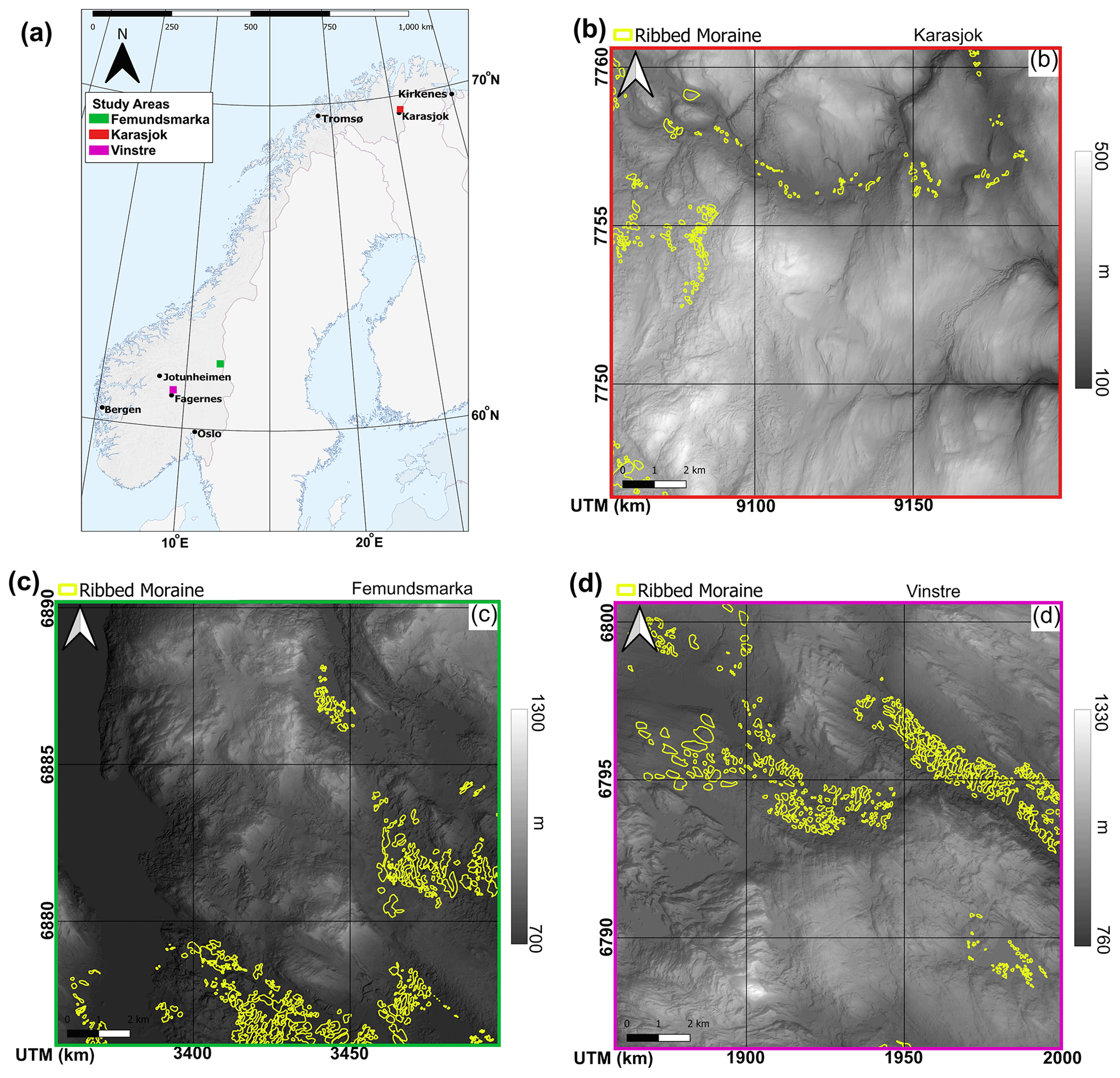
Figure 2(a) Map showing the location of the study areas throughout mainland Norway. Karasjok (b) is shown in blue, Femundsmarka (c) is shown in green, and Vinstre (d) is shown in magenta. Each location shows a submap (b–d) displaying outlines of ribbed moraines (yellow) used as ground truth in this study (Sommerkorn, 2020). Additionally, we used an area bordering the north of the site displayed in panel (d) for training the supervised methods. The basemap is made of Eurostat's GISCO administrative borders for Norway (GISCO, 2020). All maps projected in UTM 33N, EPSG:5556, and the grid projection in panel (a) uses decimal degrees while panels (b–d) use UTM 33N.
2.1.1 Random forest
The RF algorithm uses a series of decision trees (i.e. a forest) for classification, aiming to optimise the agreement with training data (Gentleman and Carey, 2008). Within each decision tree, sequences of Boolean questions subdivide the data (Breiman, 2001); the exact sequence and starting point of these questions are randomly altered for each tree of the forest. In this study, we test the RF method with 500 iterations using a majority vote method for final classification. Our RF method is trained on a small area of the known ribbed moraines to the north of the Vinstre study area. Training data here have not been used in any other component of the study and are derived from ribbed moraines mapped by Sommerkorn (2020).
2.1.2 K-means clustering
As an unsupervised algorithm, KM infers the defining parameters of each cluster based on the input data and a series of “K-centroid” points randomly scattered throughout the dataset. The algorithm clusters the most alike points around centroids through repeated iterations of the model (Fig. 3; Gentleman and Carey, 2008). KM is commonly applied in fields such as photography and medicine (Burney and Tariq, 2014; Ng et al., 2006) but, so far, has been rarely used in geomorphology (Lv et al., 2019). The ideal number of K centroids is determined after the first iteration of the model (Likas et al., 2003) by plotting the sum of squared distances within the dataset against cluster count on a chart and selecting the “elbow” point in the plotted line (Marutho et al., 2018). After the defining of the optimal number of K centroids, the model is ready for data output (Fig. 3).
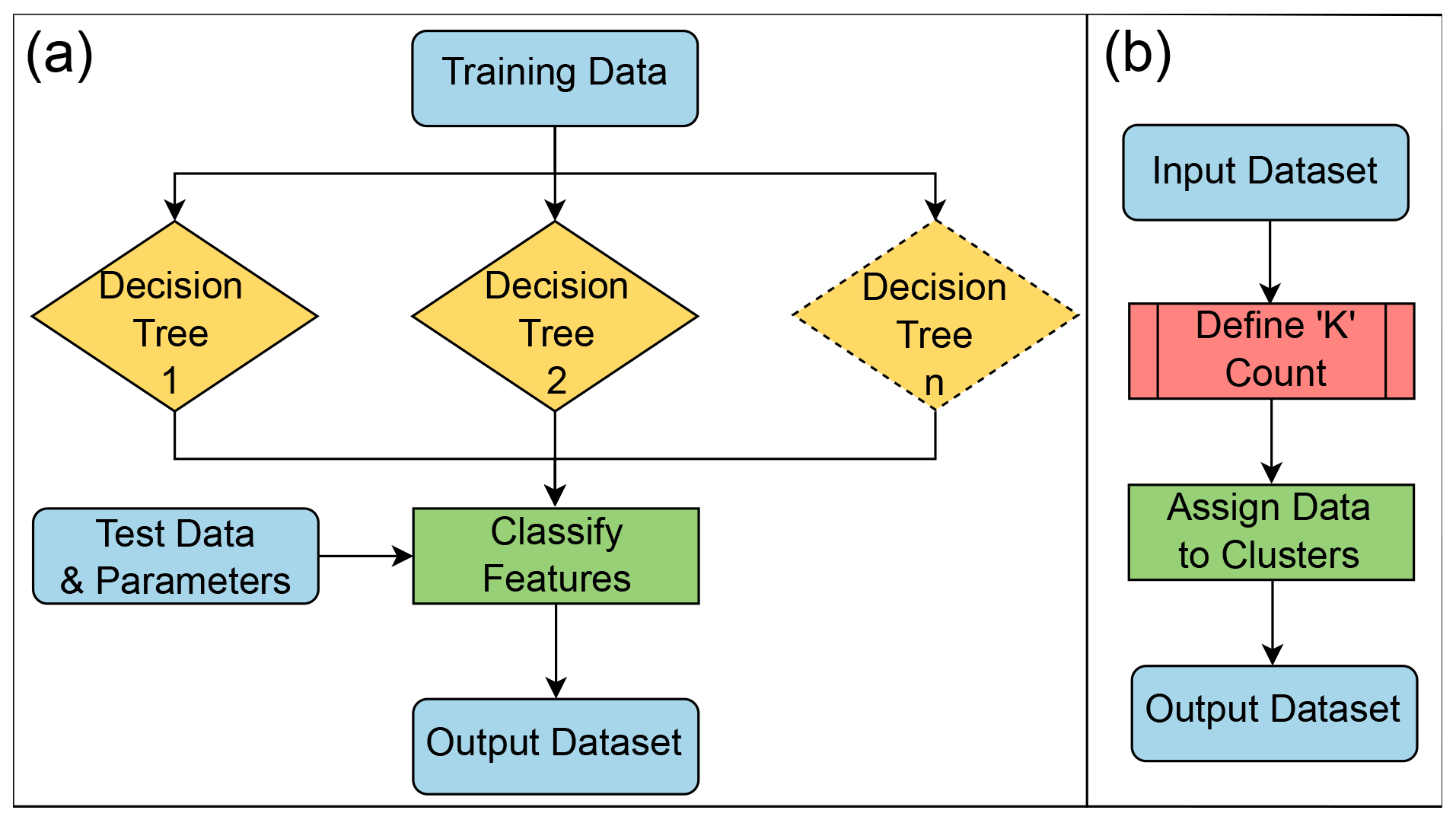
Figure 3Flow charts describing (a) the basic principles behind the RF algorithm. (b) The basic principles behind the operation of a KM methodology. The model is first run to determine the number of K points required to represent the input data and then run a second time to produce an output.
2.1.3 Outline of composite methods
We use different combinations of the above-described algorithms for three additional “composite” methods. These are designed to determine whether the limitations of individual algorithms can be overcome by combining RF and KM at the expense of time efficiency. Combined approaches are common within machine learning studies, as they can often improve performance while avoiding the micromanagement of the hyperparameters (Liu et al., 2021; Bhattacharjee et al., 2022).
The first composite method takes the output of a KM iteration to train the RF algorithm rather than providing manually delineated training data. This method was selected as one of three combination methods with the aim of minimising subjectivity from outputs, allowing RF to determine features from an automated output rather than a human-defined input. We term this method “KM-trained RF”.
The second method is defined as the “OR” method, where both KM and RF are independently performed, and the resulting classifications are merged by union; i.e. the final classification is positive if either KM or RF or both yield a positive result. This method is designed to increase functionality if one or both methods are particularly strict on feature detection or if each method functions more effectively in different areas.
The third method is defined as the “AND” method, where both KM and RF are independently performed, and the resulting classifications are merged by intersection; i.e. the final classification is positive only if both KM or RF agree. We designed this method to increase functionality in situations where one or both methods have high rates of false positives.
2.2 Method application
2.2.1 Study areas
We selected three study areas representing different landscapes present in Norway for evaluation (Fig. 2). The landscapes included are high mountain (Vinstre), heath/moorland (Karasjok), and semi-mountainous marshland (Femundsmarka). Each study area covers 15×15 km, with data at a 1 m resolution (Kartverket, 2021b). The first study area is south of lake Vinstre in central southern Norway (Fig. 2d). This region is representative of inland Norway, with a high-mountain plateau interspersed with deep glacially formed valleys (Strøm, 1948). Furthermore, high-quality ribbed moraine mapping exists in and around the Vinstre study site (Figs. 2 and 4; Sollid and Sorbel, 1994; Sommerkorn, 2020), which we use for training and validation of our methods. The second study area covers a subsection of the Femundsmarka National Park, near the Norway–Sweden border (Fig. 2c). This site is 30 km to the southwest of Lake Rogen, where ribbed moraines were initially identified and described (Lundqvist, 1969). A third study region lies in Finnmark, north of Karasjok, which is situated in a heathland and thus largely different to the former two both in form, with large rolling hills (similar in morphology to ribbed moraines), and in geology, with much less exposed bedrock.
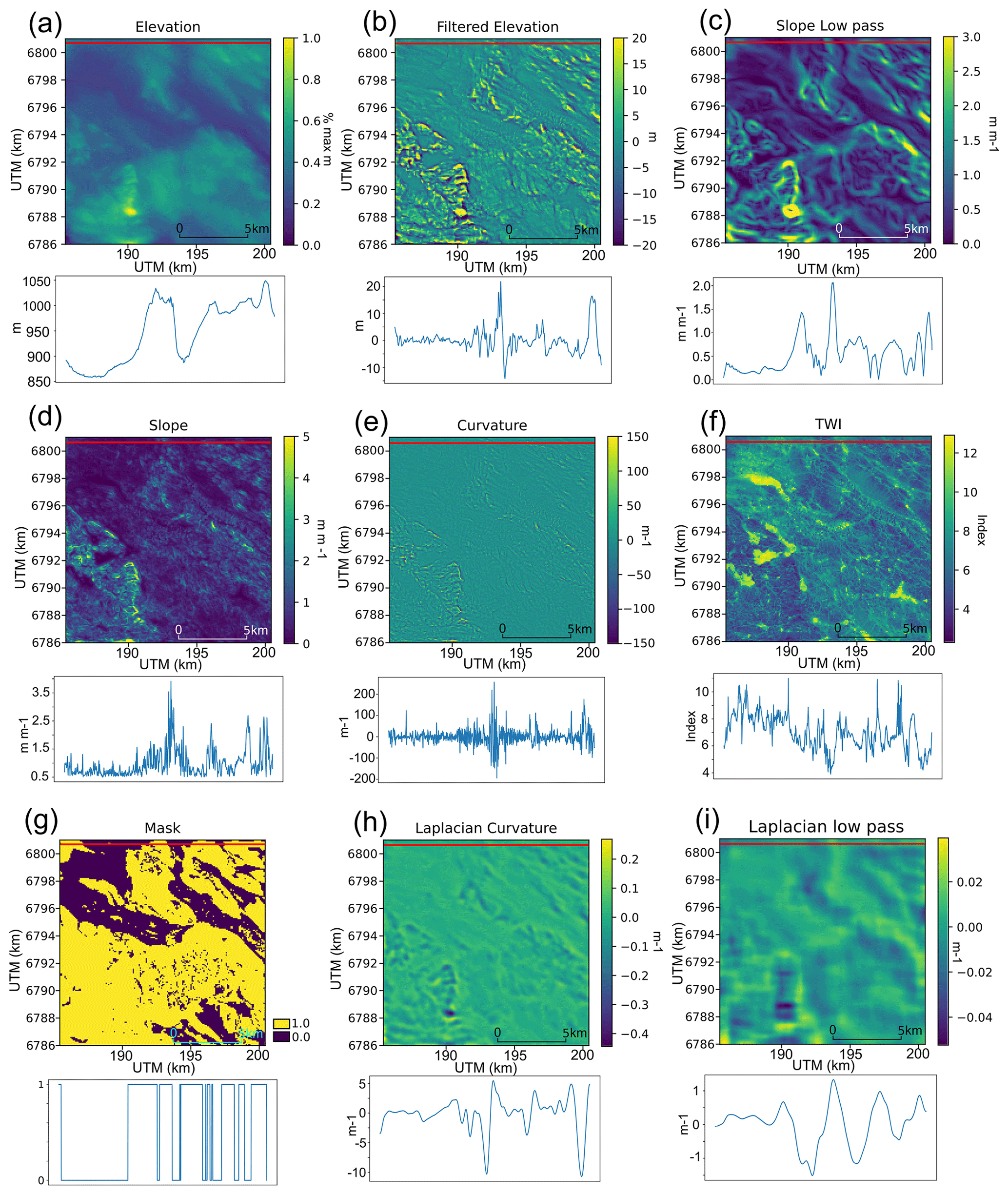
Figure 4Illustration of morphometrics used in this study, with the red line indicating the transect taken for subchart figures. Panels (a)–(f) show clustering values, while panels (g)–(i) show masking values. (a) Elevation from the 1 m resampled to 10 m DEM data (Kartverket, 2021b). (b) Elevation with kilometre-scale features filtered out. (c) The output of the general slope (low-frequency slope) filter. (d) The local slope values used for clustering. (e) Curvature values used for clustering. (f) Topographic wetness index (TWI). (g) Masking values used for excluding regions where ribbed moraine cannot form. (h) Curvature derived from a Laplacian of the Gaussian-filtered DEM for masking mountain peaks. (i) A similar plot at 1 km resolution for excluding large-wavelength features.
We trained each supervised method on a small 15×5 km subregion bordering the north of the Vinstre study area to determine the relevant parameters and morphometrics (Fig. 4). We initially tested each method on the Vinstre study region, as the terrain in the Vinstre region is highly complex and typical of inland Norway, making it useful for ensuring that the algorithm functioned well in similarly complex regions.
2.2.2 Map data
We use Norway's 1 m DEM and resample it to 10 m using bilinear interpolation for consistency instead of using an available 10 m product which was produced from various and uncertain sources (Fig. 2) (Kartverket, 2021b). We resample data for three purposes (a) because ribbed moraine occur at the scale of tens of metres, so sub-10 m data are unnecessarily detailed; (b) because without resampling the 1 m data capture too much detail in the ground surface, leading to unnecessarily detailed morphometrics; and (c) because, to limit processing time, we aim to produce a time-efficient methodology. The surface geology data are obtained as vector data from the Norwegian Geological Survey, NGU (NGU, 2022) and lake vector data from the Norwegian Water Resource and Energy Directorate, NVE (NVE, 2023). We used the nearest-neighbour interpolation to convert these vector datasets into 10 m raster data, matching our resampled DEM. We obtained orthophotographs from Norway in pictures (NiB) (Kartverket, 2021a, c) and use this for ground-truth production and qualitative output validation. In addition, we use existing geological maps and mapped ribbed moraine ridges from Sommerkorn (2020).
2.2.3 Derived data
We use our raw data for two purposes, namely to produce training/testing datasets and to generate morphometric and mask attributes for our machine learning algorithms. We manually delineated training/testing ground truth data using a combination of previous moraine maps, the 1 m DEM, and orthophotographs. We find that ribbed moraines in marsh areas are easily identifiable in orthophoto imagery due to their distinct contrast in colour to their surroundings; however, in forests they are not detectable due to tree cover (Dunlop and Clark, 2006).
We derived morphometric and masking data from the DEM using several modules: the RichDEM Python module (Horn, 1981; Zevenbergen and Thorne, 1987; Barnes, 2016), SAGA (Conrad et al., 2015), and the opencv Python module (Bradski, 2000). We also produced several filtered DEMs from the input 1 m DEM including a 400 m low-pass filter, a 30 m high-pass filter, and a 30–400 m bandpass filter designed to isolate the size scale of ribbed moraines as defined by Dunlop and Clark (2006). For our topographic wetness index (Böhner et al., 2001) data, we calculated indices using local values derived from the input DEM rather than global.
2.3 Morphometrics
We first select morphometrics based on the basic observable characteristics of ribbed moraines. In addition to the filtered elevation data (30–400 m; Hättestrand and Kleman, 1999; Dunlop and Clark, 2006), we generated the slope, general slope, curvature, planform curvature, profile curvature, spatial distribution (wavelength), and aspect. In addition, we derived the topographic wetness index (Böhner et al., 2001; Conrad et al., 2015) and topographic position index (Guisan et al., 1999) as metrics with the potential to add value to the segmentation algorithm. Each morphometric was identified from prior literature (e.g. Eisank et al., 2014) and qualitatively tested for its ability to isolate ribbed moraine. With the combination of the best-performing morphometrics, we suggest the possibility of differentiating ribbed moraines from other landforms.
Second, we selected masking values to remove as much noise from the input data as possible and avoid obvious misclassifications. This also aids our accuracy metrics by improving the balance of our data, as both RF and KM work most successfully on balanced data rather than unbalanced data (Pedregosa et al., 2011). Here, the best-balanced data are defined as data for which there is roughly a split in the count of pixels per binary output category. Hence, masking values are used to remove as many pixels as possible in situations where ribbed moraines do not or cannot form, balancing the dataset somewhat. From consulting the literature, we defined areas where ribbed moraines cannot form as mountain peaks (Hättestrand and Kleman, 1999), steep slopes (Sommerkorn, 2020), and where surface bedrock is present (Sommerkorn, 2020). We also defined lakes as areas in which ribbed moraines are not detectable using DEM data. For each of these limitations, we produced a mask layer. Large-scale (over 1 km) peaks and ridges are masked from the dataset by setting a threshold on a Laplacian of Gaussian filter. The Laplacian of Gaussian is a second-order derivative edge detection filter which identifies regions that show sudden steep changes in intensity (Kong et al., 2013). We mask steep slopes using a generalised slope layer generated from a low-pass filtered DEM (over 400 m); slopes with inclines greater than the thresholding value (e.g. Table 2) were masked out of the dataset. The low-pass filtered DEM is used together with a slope angle threshold to mask out the general valley slope angle. Additionally, we mask mountains of a set wavelength from the testing to omit plateau edge convex surfaces from the analysis using a simple sinusoidal Laplacian filter (Kong et al., 2013) referred to as a “mountain wavelength mask”. In this case, mountains with a wavelength of greater than the threshold value were filtered out of the dataset. To mask out areas of exposed bedrock, we used the national surface geological map of Norway (NGU, 2022) and masked all areas defined as exposed bedrock. Finally, we used NVE's lake database to mask out lakes (NVE, 2023).
Method outputs were visually compared to the locations of ribbed moraines as defined in Sommerkorn (2020). We made qualitative visual comparisons here as the changes made by different morphometrics were large, with numerical analysis occurring as part of later predictor tuning. We made our visual comparisons against high-resolution orthophotography (Kartverket, 2021a, c) and Norway's 1 m resolution national DEM (Kartverket, 2021b). We then adjusted the algorithm to produce the most visually accurate output with the fewest inputs. Hence, in developing the method, we removed the aspect as it made no notable contribution to the output. We also conflated both planform and profile curvature into the total curvature metric, as we observed no difference in the output from any singular curvature parameter. In testing the value of the literature-defined morphometrics, we found the topographic wetness index to be highly useful but also found the topographic position index added no value to the output in any combination.
2.4 Workflow in practice
We implemented the series of segmentation algorithms on the combination of raw and derived data. We began by pre-processing the datasets to fit with each chosen study area as defined by the borders of the associated 1 m resolution DEM tile (Fig. 2). Once pre-processed, we ran each test algorithm on the datasets for Vinstre, Femundsmarka, and Karasjok. We also carried out a second iteration of RF using KM-produced training data and combined outputs from KM and RF to produce each of our composite method outputs. Once we had completed each method, we prepared output datasets for statistical analysis via a standard confusion matrix (Fig. 5).
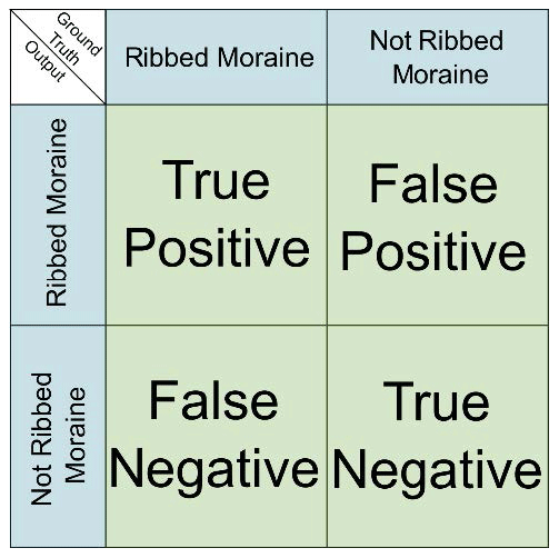
The first metric to test each method was efficiency – defined as the required CPU time. Then, we measured the effectiveness of each method in detecting ribbed moraines. For each of the five methods, we derived the confusion matrix, stating the numbers of true positive, true negative, false positive, and false negative pixels and comparing model outputs to the manually delineated ground truth data (Fig. 5; Hong and Oh, 2021).
2.5 Comparative analysis
In addition to producing a visual representation of each method's effectiveness (Fig. 4), we calculated accuracy metrics of the balanced accuracy (BA; Eq. 4; Brodersen et al., 2010) and F score (Sokolova et al., 2006), each of which represents different sides of the confusion matrix and each ranging between 0 and 1. We selected the BA and F score over a standard accuracy metric (Eq. 1) as the standard accuracy is skewed positively in unbalanced datasets. As our dataset comprises regions where ribbed moraine do not make up 50 % of the mapped area, our data can be considered unbalanced; hence, we make use of BA. To calculate BA, we use Eq. (4).
BA accounts for the imbalance between classes, and it works effectively in identifying the influence that positives have on the accuracy of a dataset; hence, a higher BA score represents a dataset with good positive returns versus ground truth. The F score is computed as the harmonic mean of precision (Eq. 5) and recall (Eq. 6).
The F score ignores true negatives and, like BA, works well on imbalanced datasets. The F score typically will be higher when there are lower false positive and false negative values, as it pays less attention to true positives and true negatives than BA. Therefore, in working with both metrics, we gain a detailed understanding of the accuracy of our output.
2.6 Final algorithm adjustments
Once we identified which algorithm provided the best combination of effectiveness and efficiency, we improved the performance by adjusting the models' parameters. We took two approaches to make these adjustments: systematic and intuitive. For systematic improvements, we adjust parameter values in small increments over a physically plausible range; the general slope mask threshold values are adjusted by 0.01 from 0.65–0.75, the Laplacian curvature mask threshold values are adjusted by 0.005 from 0.04–0.08, the general slope kernel size is adjusted by 10 m from 300–400 m, and the mountain wavelength masking is adjusted by 100 m from 1 to 2 km (Table 2). These tweaks thus provide an objective analysis of outputs based on pure accuracy scores.
For our intuitive approach, we changed inputs with the aim to maximise the visual agreement between the classification and the evaluation data. This approach served as a health check of our dataset, ensuring that our method specifically detected ribbed moraines rather than resorting to “detection by accident”. We used both approaches as a means of performing a robust sensitivity analysis, ensuring that specific landforms were detected. In certain situations, many pixels of ribbed moraines may be identified, but many conjoining pixels could also be detected as “ribbed moraine”, thus only detecting ribbed moraine fields rather than discrete landforms. Hence, while we aim to use the systematic analysis to determine the parameters with the highest statistical accuracy, we used the intuitive analysis to determine the parameters which lead to the highest accuracy scores while still detecting discrete landforms rather than fields. The intuitive analysis involved changing the same parameters as in the systematic tweaks while also changing cluster counts by ±1 and making minor adjustments at the scale of 10 m to the filtering kernel size used on the DEM.
3.1 Comparative method results
Our segmentation methods were quick to run (10–60 s) and produced reasonable outputs on a mid-range laptop (Intel i5-1135G7; 2.40 GHz, 2420 MHz, and quad-core processor; Intel Iris Xe Graphics; 16 GB and 3200 MHz RAM). However, the outputs varied greatly between methods and study areas. As such, we separated our results between each segmentation algorithm and study area and then outlined the mean results between each study area for each method.
3.1.1 Vinstre
In our test and evaluation of the five chosen methods at Vinstre, we find reasonable outputs for each method, thus showing the capabilities of detecting ribbed moraines in the terrain of this region (Fig. 6). However, each algorithm varies through its false positive and false negative detection rates. The standard accuracy (Eq. 1) values (Table 1) show accuracy to be over 88 % for all methods, with a mean of 0.926. However, due to the natural imbalance of our data, this metric is largely dominated by the abundance of negatives. We expected some exaggerated false positive detection, yet some methods are better than others at omitting this. In addition, some of the methods detect more false positives than others, which is more difficult to exclude from the dataset. For example, we can see that KM and OR outputs show consistent false positives on the rounded peaks in the Vinstre study area's south, while the KM-trained RF algorithm shows a widespread pattern of random false positive detection (Table 1). The RF and AND methods yield fewer positive pixels overall, which leads to lower accuracy scores, as only the banks or ridges of ribbed moraines are detected rather than full features.
Table 1Performance scores for each study area (Fig. 6); metrics are rounded to three decimals. As the BA and F score are combinations of recall and specificity (Eqs. 2 and 3), we only include the BA and F score outputs in this table.
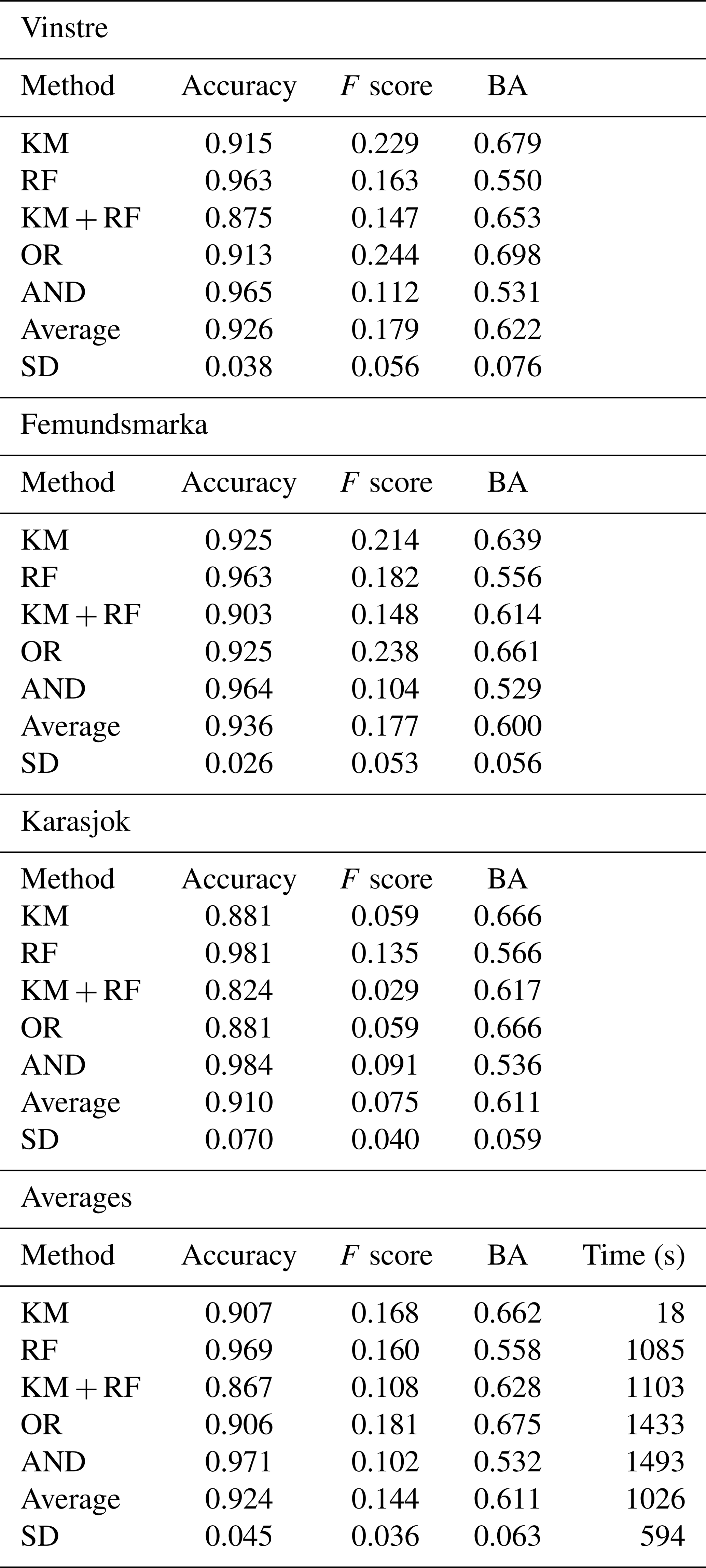
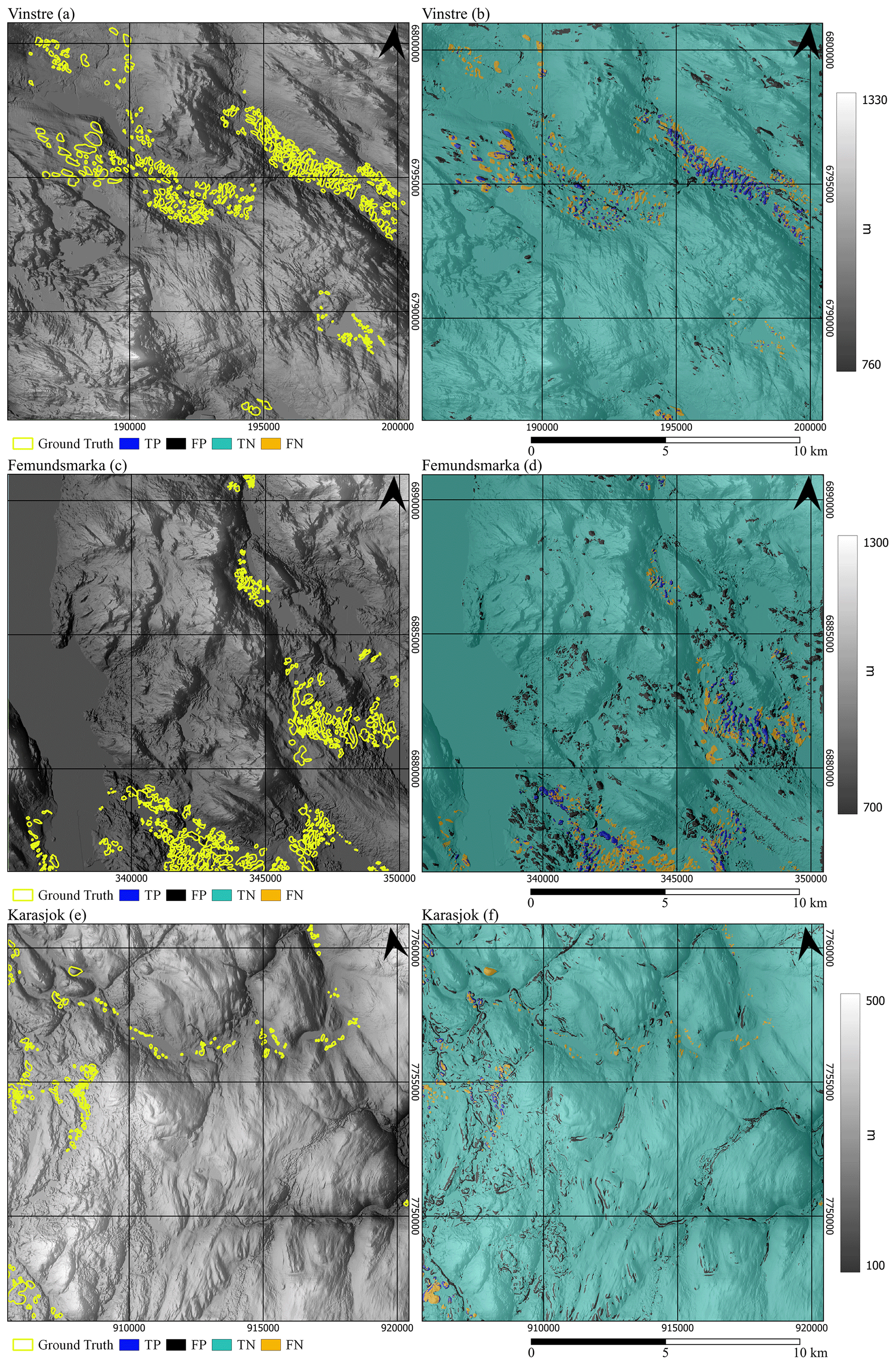
Figure 6Comparison of input to output in the three study regions. Panels (a), (c), and (e) show ground truth data, while panels (b), (d), and (f) show accuracy maps denoting confusion matrix (Fig. 5) values for the clustered output of the KM method. Outputs are superimposed on a hillshade of the input DEMs (Kartverket, 2021b).
Statistically, we find the KM and OR methods to have the highest and most consistent accuracy metrics, suggesting that these methods have the most use in ribbed moraine detection. We see this with KM returning BA of 0.75σ (standard deviations) above the mean and F scores of 0.89σ above the mean (Table 1). The OR output echoes this with BA and F values of 1.16 and 1.00σ above the mean, respectively (Table 1; Fig. 6). On the other hand, while the AND approach is the second most effective method in terms of overall accuracy, we see poor results in balanced metrics, giving values of 1.20σ below the mean value. Furthermore, the KM-trained RF method shows the least promising visual output and the least consistent and near-least promising accuracy output, where accuracy = 1.34σ below the mean, BA = 0.57σ below the mean, and F score = 0.41σ above the mean (Table 1). Therefore, as an overall ranking, we rate the OR method as the best performing in the Vinstre region, while the KM-trained RF method returns the least successful results.
3.1.2 Femundsmarka
On comparing results from Femundsmarka, we find a similar pattern to that of Vinstre, with high false positives and negatives common between the KM-trained RF. Additionally, RF and AND classifiers showed distinct features in qualitative detection. The false positive detection of rounded hills in the Femundsmarka region is reminiscent of the Vinstre region in the KM and OR classifiers. We also rank each method the same as for the Vinstre site, while also showing that the variation in the performance from the mean is similar between both sites. We find that major differences are only present within the KM-trained RF method and the RF method in terms of variability. For these, the KM-trained RF returns values of 1.27, 0.55, and 0.25σ below the mean for accuracy, F score, and BA, respectively. RF, on the other hand, returns 1.04, 0.09, and 0.79σ above the mean. In this case, we see that the KM-trained RF method consistently trended towards below-mean performance, whereas RF consistently performs above average.
3.1.3 Karasjok
Performance patterns in the Karasjok region depart from those in the previous areas. There is greater variability between algorithms and a general increase in misclassifications. The RF and AND methods perform well in Femundsmarka and Vinstre, while the KM, KM-trained RF, and OR methods produce outputs with speckled pixels. Many false positives are present, particularly in the southern part of the Karasjok region. It is likely that these false positives are a result of different landscape morphologies between Vinstre, Femundsmarka, and Karasjok, where the latter is a moorland environment, which is different compared to the prior two that are more typical of inland Norway (Hjort et al., 2014). Statistically, we also see the poor performance of KM rates below the mean standard accuracy and of F score metrics by 0.40σ, while maintaining a high BA score of 0.93σ above average (Table 1). In short, this means that KM is effective at detecting true positives but classifies too many false positives. RF is opposed to this, with the accuracy and F score returning values of 1.01 and 1.50σ above average, respectively, compared to 0.76σ below average for BA. The OR method returns identical values to KM, as RF under-classifies features in the Karasjok region, thus allowing KM to dominate the OR output in this area.
Despite the differences in the Karasjok region, we still see similarities between the Karasjok region and the prior two, with both the KM-trained RF and AND approaches having inconsistent variability from the mean, suggesting their lack of value as methods. Due to the locality of the false detections found in the KM and OR methods, it is possible that they are detecting features common to this region which likely have a similar form to ribbed moraines found elsewhere in Norway.
3.1.4 Overall performance
Studying the overall performances of each method across the different study sites, we find similar results in the first two regions, where KM ranks consistently second in BA, and OR ranks highest. KM performance scores are both above average by 0.38 and 0.81σ, while all other methods show some inconsistency between accuracy metrics. For example, the OR method ranks 1.02–1.03σ above the mean BA but ranks 0.40σ below the mean performance. Hence, while KM does not rank as highly as OR in BA, its output is more consistently accurate. As a result, we can discount the combined, RF, and AND methods, as they all consistently rate third or worse in accuracy metrics, showing their lack of segmentation effectiveness.
In addition to accuracy, we determined the CPU time required for each method (Table 1) as a measure of efficiency. On a mid-range laptop (Intel i5-1135G7; 2.40 GHz, 2420 MHz, and quad-core processor; Intel Iris Xe Graphics; 16 GB and 3200 MHz RAM), KM takes only 18 s on average per iteration, which is 1.67σ faster than the mean rate, while every other approach takes 2 orders of magnitude more time at over 1000 s. When considering our two most statistically effective methods, we find KM is notably faster than the OR methodology. Due to its much lower computational cost, we selected KM as the method of choice, despite its slightly lower performance.
3.2 K-means refinement
Upon producing a baseline set of predictors for the KM methodology, we conducted many predictor adjustments as a sensitivity analysis. These values aided in determining two final “best-fit” methods based on statistics through a systematic approach and statistics combined with qualitative observations made on the output maps.
3.2.1 Systematic analysis
The systematic analysis yields optimal predictor values in terms of average BA scores for each iteration per region. For example, the optimal value of the general slope threshold is 0.71, where BA values are 0.76, 0.61, and 0.72 for the Vinstre, Femundsmarka, and Karasjok sites, respectively. The optimum BA scores 1.7σ above average for the range of tested values (Table 2).
Table 2Table showing the predictor values from systematic analysis with BA as the key accuracy score. BA range shows the range from minimum to maximum values of BA output. Each predictor was tested on an individual basis.
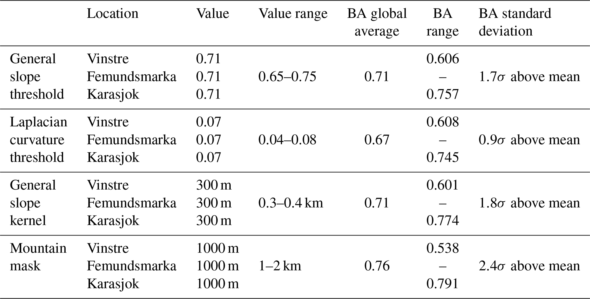
In addition to our best outputs, we note interesting values and themes throughout the systematic analysis. In general, we found each region to have similar patterns of maximal performance. The only commonality between our three sites under the general slope kernel value tweaks was with a parameter value of 300 m (where the kernel size for slope smoothing is 300 m resolution), where all scores were above 0.64 BA. The pattern of scores calculated using 300 m general slope kernel (0.74 Vinstre, 0.65 Femundsmarka, and 0.73 Karasjok) is common throughout this parameter's output. While Femundsmarka generally follows the pattern of values in the other two datasets, changes are more muted, with values ranging between 0.61 and 0.67 for the general slope kernel, general slope threshold, and Laplacian curvature threshold compared to changes that are double this magnitude in the Vinstre and Karasjok regions. Furthermore, while there is general agreement throughout the data, Vinstre appears to be at odds with respect to the optimal values at Karasjok for accuracy scores in Laplacian curvature threshold tests, with the optimal values having no relation.
The tweaks made to the mountain wavelength mask present much more varied results than the other tests, but a consistent optimal or near-optimal value is seen. This lack of consistency is likely due to the different wavelengths of the mountains in each study area. But additionally, it appears that a consistent wavelength for mountain features is roughly 1 km between the trough and peak. Our results clearly show this, with maximum BA values of 0.79 (Vinstre), 0.76 (Femundsmarka), and 0.73 (Karasjok). This high performance also means that the mountain mask parameter is the most influential parameter on statistical detection, improving the mean BA across the board by 0.10 (3.6σ above the mean improvement). On the other hand, the least influential parameter is the Laplacian curvature threshold, with an improvement in accuracy of only 0.03, which is only 0.9σ above the mean BA score. This result, however, is consistent with the lack of agreement between datasets when tweaking the Laplacian curvature threshold value.
3.2.2 Intuitive approach
Results from our intuitive analysis show several outputs with high BA. Each of these approaches yields BA scores > 0.70 at Vinstre and a mean of >0.69 across all regions. Yet, a visual evaluation reveals that settings in which the BA score is >0.70 can lead to moraine overclassification (Fig. 6). Thus, despite the high BA, this validates our health check, demonstrating that higher statistical performance does not necessarily produce the best-performing output for discrete feature detection. This potentially comes from the complexity of the terrain in which we iterate the method, with areas of higher relief generally performing worse than lower relief when using geomorphometric methods (Hjort et al., 2014). In short, we find BA < 0.70 leads to a discrete detection of ribbed moraines, while BA > 0.70 delineates ribbed moraine fields, filling the gaps between features. Hence, we outline two potential approaches, namely (1) that high accuracy should be the focus, aiming to detect fields of ribbed moraines as in previous studies, and (2) that discrete ribbed moraines should be the focus, aiming to detect individual ribbed moraines on a large scale.
We also note several patterns between our analysis approaches. First, we find less agreement between all three regions in the statistical output of our trial-and-error intuitive approach versus the systematic approach. Despite this, we also find that there is consistent agreement in our most effective discrete landform detection method, with scores varying by <1σ. Interestingly, we find that, again, Femundsmarka shows the lowest variability in the BA score, with a standard deviation of 0.29σ versus a standard deviation of 0.50σ for Vinstre and 0.56σ for Femundsmarka.
4.1 Pre-predictor tuning
The high level of agreement with the ground truth in the Vinstre region shows the KM algorithm's potential. Through F score and BA, we find the KM method to be most successful in the Vinstre study area, likely due to the method being originally initiated on the complex mountainous terrain of inland Norway. This is promising because it shows that the method performs well at detecting ribbed moraine in regions of high relief, which is one of the most common areas for ribbed moraine to form (Sollid and Sorbel, 1994; Sommerkorn, 2020). Hence, we assert that this method is transferrable throughout central Norway and other similarly mountainous regions. Yet, we find the main shortcoming of the pre-tuning method in the Vinstre study region to be the overdetection of riverbanks, palaeo-channels, and other morphologically similar landforms. This is potentially in part due to the interpolation of 1 to 10 m data averaging the morphometric signals.
We additionally find good performance in the Femundsmarka study area, with an F score of 0.21. This is most likely due to the partial similarity to the Vinstre study area with the presence of some high-mountain terrain. However, complexity in the local relief increases, including three terrain types, moorland, lake, and high mountain, versus the consistent high-mountain terrain of the Vinstre study area. While lakes are masked out, the mixed semi-mountainous marshland of Femundsmarka likely contributes to the lower-accuracy scores due to transferability issues between different reliefs (Hjort et al., 2014), as Femundsmarka's results show the algorithm attempting to classify the lakeshore and rounded moorland hills as ribbed moraine (Fig. 6d). This reflects the riverbank detection in Vinstre and thus is most likely due to the similarity of morphology, particularly in relation to the slope and curvature (Dunlop and Clark, 2006; Lindén et al., 2008; Möller, 2006). Additionally, Femundsmarka shows greater rates of false negatives than Vinstre, with many ribbed moraines in the south of the study area (Fig. 6d) being unclassified. The cause of the false negatives is unclear, but they could be attributed to the lower overall difference in elevation between the ribbed moraines and their surroundings (30–40 m north, 20–25 m south) in southern Femundsmarka. Despite some of the limitations, we consider our initial results from Femundsmarka promising.
With an F score of 0.06, Karasjok has a greater rate of false positives than other regions (Fig. 6). This may be a result of the landscape being predominantly comprised of rounded hills with a similar appearance to ribbed moraine (similar to areas of Femundsmarka). BA is 0.67, in comparison to the 0.64 and 0.68 for Femundsmarka and Vinstre, respectively. Hence, the primary issue with the Karasjok region is overdetection (increased false positives). We propose the issues of false positive detection that we observe in Karasjok to be a result of inherent transferability issues that arise in geomorphometry. Hjort et al. (2014) describe the difficulty in extrapolating geomorphometric methods from high- to low-relief areas, as region-specific conditions can have a strong impact on the relative importance of different variables. In the case of Karasjok, the change in relief likely leads to a greater influence of the curvature metric. Alternatively, this could be a product of the interpolation between 1 and 10 m, leading to an inaccurate curvature value for channel features.
The overdetection we observe in our study regions could be limited by predictor tuning (Moradi Fard et al., 2020) or through classifying detected features post-detection. For this study, we choose to take a consistent approach and undergo predictor tuning to improve our methodology, due to the initially promising output from our approach.
4.2 Finalised outputs
4.2.1 Computation considerations
For all iterations, we found that the relatively light computing load opens the possibility of applying the method to larger scales such as mapping ribbed moraines all over Norway. In addition, the parallelised implementation of K-means, named “minibatchkmeans” (used in this study) (Pedregosa et al., 2011), further increases the processing speed on multicore servers.
4.2.2 Performance
In computing BA, we find reasonable (0.59) to good (0.78) scores, depending on iteration and location. Mean BA scores vary by 0.11 (0.60 to 0.71), which we expect given the varied terrain types. This outlines issues in transferring between terrain types and maintaining performance. For example, during our systematic analysis, we set the general slope threshold to 0.75 and find BA values of 0.63 (Vinstre), 0.62 (Femundsmarka), and 0.73 (Karasjok), demonstrating better performance in the Karasjok moorland than in high-mountain terrain. Due to discrepancies between what can be considered valuable in qualitative versus quantitative results, BAs below 0.75 do not suggest poor method performance, as values between 0.65 and 0.70 show the greatest performance in this study for detecting discrete ribbed moraines. It is, therefore, important to consider that the algorithm is not designed to detect ribbed moraine but “ribbed moraine-like” features. This means that there will always be a degree of over-/under-classification, particularly in complex post-glacial and real-world landscapes due to the variability in the ribbed moraine shape (Dunlop and Clark, 2006). We will also see over-/under-classification due to geomorphological features of a similar shape within our study areas, as ribbed moraines do not develop in isolation (e.g. drumlins, channels, and mega-scale glaciolineations; Ely et al., 2016). Hence, over-/underdetection can be perceived positively, as output features can be classified post-detection using parameters such as orientation versus glacial streamflow, where ribbed moraines are perpendicular and drumlinoid forms are parallel to this (Dunlop and Clark, 2006; Ely et al., 2016).
Second, we find that BAs below 0.70 may be of greater value than those above 0.70 if we are aiming to identify discrete features. Our results show that BAs of more than 0.70 present more true positives, resulting in good statistical results, but many more false positives are also present, as spaces between ribbed moraines are detected as ribbed moraine. This results in areas between ribbed moraine being filled up, leading to a positive detection of moraine features, but discrete ribbed moraines are poorly captured. Hence, we consider a range of results as successful, i.e. BA 0.65 to 0.75, depending on whether the aim is to classify fields or discrete landforms. This is due to BA alone not being the ideal parameter for measuring the value of our output – but instead we require complementary assessment, through qualitative analysis as a means of determining output value, on top of the ideal range of BA values. We thus believe both sets of BA scores are reasonably accurate, particularly as our raw accuracy never drops below 0.82, representing an 82 % per pixel success rate.
4.2.3 Transferability
The transferability of this algorithm depends on one major component: the widescale landscape type and relief, showing similar issues with transferability to previous works (Hjort et al., 2014). We find that the method works well when applied to similar landscape types, as seen in Femundsmarka and Vinstre. When transferred to different landscape types and reliefs (i.e. between high-mountain, moorland, and mixed marsh–mountain terrain), we observe a poorer detection of ribbed moraines. As a result, this algorithm is transferable for most landscapes where ribbed moraines occur in inland Norway (high mountain); however, for regions exhibiting differences to the high-mountain regions, such as moorland and coastal regions, we can tune the model accordingly at the scale of each DEM tile. This is relevant when considering expansion to other regions of the world, as much of the Canadian shield is landscape close in format to Karasjok – which would indicate a need for predictor tuning (Dunlop and Clark, 2006; Dunlop et al., 2008).
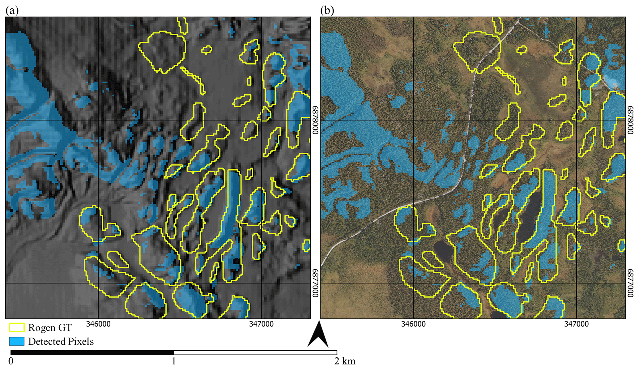
Figure 7Comparison of ground truth to detected pixels on (a) hillshade and (b) orthophoto imagery (Kartverket, 2021a, c). Here, GT refers to ground truth.
4.2.4 Detection of new features
While analysing our outputs, we found evidence of ribbed moraines detected by the algorithm that was not present in the ground truth data. These ribbed moraines were commonly found in the Femundsmarka region, in areas adjacent to manually marked ribbed moraine (Fig. 7). The detected landforms occur in small clusters with a similar pattern to ribbed moraine, as described in Dunlop and Clark (2006). We suggest that this may be due to a series of factors, including the presence of forest and farmland, obscuring ribbed moraine in stereo-imagery or poor DEM data used for the manual production of ground truth data. Hence, we suggest that while the method has some limitations, there are also clear advantages, as the method uses lidar data, which does not exhibit the same issues in differentiating between landforms under forest cover as spectral imagery.
4.2.5 Last Glacial Maximum (LGM) ice flow direction proof of concept
To explore possibilities for further refinement, we calculated the orientation of each detected polygon using a simple bounding box method and determined the orientation of its longest axis. We compare these orientations with modelled flow direction of the FIS (Fennoscandian Ice Sheet) by comparing feature orientation to the mean flow direction of the ice sheet between 11 and 25 ka (Patton et al., 2016, 2017). Figure 8 shows polygons perpendicular or streamlined (±25°) to glacial flow, which are helpful in distinguishing landforms oriented the along flow direction (drumlinoid) from those oriented transverse (ribbed moraines) to the flow direction. Yet, we note limitations with hummock forms (Ely et al., 2016), as they have no dominant orientation and could end up in any group, demonstrating a need for a more robust classification method potentially based on the feature aspect ratio. We also note that this method has challenges in detecting the orientation of anastomosing features, a common type of ribbed moraine (Dunlop and Clark, 2006). Another potential limitation of this method is the low resolution of modelled glacial flow, which is of the order of kilometres and wider than many glacial valleys.
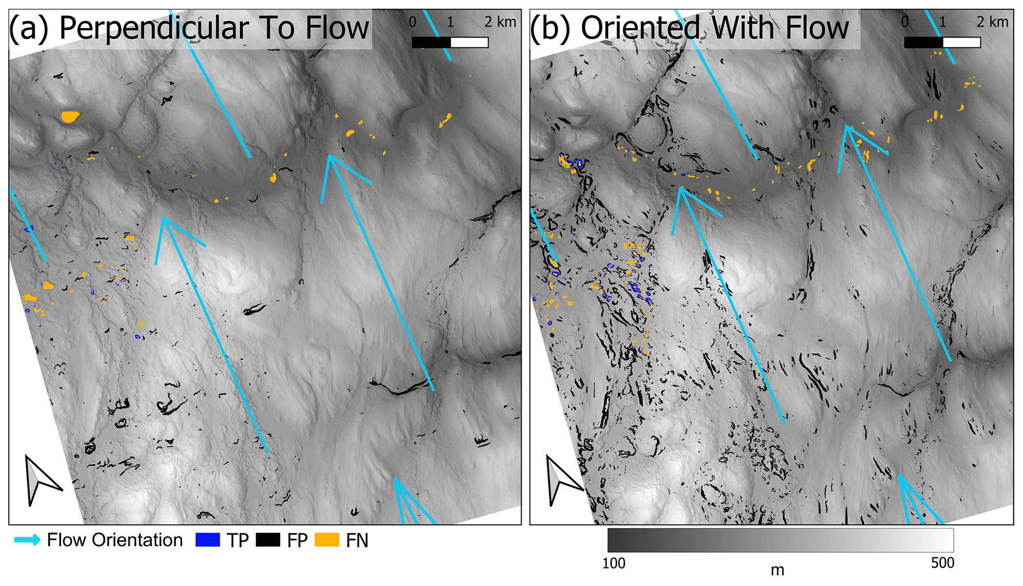
Figure 8Detected features versus LGM ice flow direction in the Karasjok region. Panel (a) shows values ± 25° from orientation perpendicular to the mean flow direction (blue arrows) during the FIS (Fennoscandian Ice Sheet) (Patton et al., 2016, 2017), and panel (b) shows values not oriented perpendicular to the average flow angle during FIS (Patton et al., 2016, 2017). Both figures are superimposed on 10 m DEM and hillshade (Kartverket, 2021b).
4.3 Avenues for method improvement
We identified two areas of improvement. First, we suggest improving automation, which would allow scaling to larger areas. For example, through the inclusion of automated predictor tuning for landscape types in the model parameters (parameter profiles). Automation would allow for application on a country scale with minimal input through the implementation of these parameter profiles, thus minimising false positive and false negative identification in varied landscapes. We envision four landscape types for Norway: high mountain (our original approach), low mountain, moorland (Karasjok), and coastal. We believe that these four categories would cover the main landscape types common across regions where ribbed moraines are present. These categories would likely prove sufficient in the regions outside Norway where ribbed moraines are known to exist (e.g. Canada, Ireland, United Kingdom, Sweden, and Finland); however, regional differences in scale and geology may require the parameterisation of the landscape type.
Second, we identify the importance of implementing a post-detection classification of landforms. Our results show that overclassification is common, particularly as there are many landforms with similar geomorphological properties to ribbed moraines (Fig. 6). We suggest future works include an investigation into landform classification, as it would allow identifying specific landforms including drumlinoid forms, ribbed moraine, and others, thus improving the value of the methodology. This would potentially aid the continuum hypothesis of Ely et al. (2016) by showing landform transitions from ribbed moraine. Hence, we consider this as the next logical step in method development. In addition, we suggest that, with post-detection classification, this method could be used on a wider basis than only ribbed moraine, due to its ability to easily detect specific geomorphologies based on relatively basic morphometric traits.
To develop a method for automated mapping of landforms throughout Norway, we tested two machine learning algorithms and three composite approaches. We determined ribbed moraine as a suitable example landform which would also be scientifically interesting to identify. Through testing, we settled on using an unsupervised K-means clustering algorithm for moraine detection, thus requiring no training data. Ground truth data for our testing were produced through manual analysis of high-resolution elevation model (Kartverket, 2021b) derivatives and high-resolution aerial/satellite imagery (Kartverket, 2021a, c).
Our results demonstrate unsupervised machine learning as sufficient for the automated detection of geomorphological features through a simple KM approach, rather than the need for complex supervised machine learning methods. We also demonstrate that minimal data are needed for this approach, with only high-resolution DEM derivatives, superficial geology, and a lake mask required for our methodology to function. We evidence this in the initial testing, where a supervised RF method averaged poorer performance than an unsupervised KM approach. In addition, we find that we can differentiate between the identification of discrete landforms and fields of landforms. Hence, we find this method to be scalable in that different output resolutions are possible.
This study indicates the value of automated machine learning for landform detection as a means of minimising time spent delineating features manually and in-field. We detect ribbed moraines throughout our study areas in relation to ground truth data and detect a small number of previously unmapped ribbed moraines in one of these. Thus, we show the value of an objective and systematic method using new, high-resolution data in detecting features. Furthermore, we detect many additional features in all study areas which have similar morphologies to ribbed moraine, but powerful refinement can be achieved by considering orientation with respect to the former ice flow direction.
In summary, this study demonstrates that unsupervised machine learning is a viable and efficient method for the automated detection of ribbed moraines and similar features based on modern high-resolution DEM (Kartverket, 2021b). With our promising results, we identify a future path for such methodologies in geomorphology as a means of updating geomorphological maps and producing new geomorphological maps where we have high-resolution data to input (e.g. dune mapping on Mars). Thus, we intend to develop this work into mapping ribbed moraine and adjacent features throughout Norway, so as to aid in developing our understanding of the geological history of Fennoscandia.
The finalised code is available in the repository Aeteia/Ribbed-Moraine at https://doi.org/10.5281/zenodo.7991094 (Barnes and Filhol, 2023).
The supporting data produced for this paper are openly available in the repository Aeteia/Ribbed-Moraine at https://doi.org/10.5281/zenodo.7991094 (Barnes and Filhol, 2023). The input data for this paper are freely available and can be found in the Norwegian national geospatial data archive at the following links: NiB (http://opencache.statkart.no/gatekeeper/gk/gk.open_nib_utm33_wmts_v2?SERVICE=WMTS&REQUEST=GetCapabilities, Kartverket, 2021a; http://data.europa.eu/88u/dataset/dcee8bf4-fdf3-4433-a91b-209c7d9b0b0f, Kartverket, 2021c) at http://opencache.statkart.no/gatekeeper/gk/gk.open_nib_utm33_wmts_v2?SERVICE=WMTS&REQUEST=GetCapabilities, national 1 m DEM (Kartverket, 2021b) at http://data.europa.eu/88u/dataset/dcee8bf4-fdf3-4433-a91b-209c7d9b0b0f (Kartverket, 2021b), lake database at https://www.nve.no/kart/kartdata/vassdragsdata/innsjodatabase/ (NVE, 2023), surface geology map (NGU, 2022) at https://gisco-services.ec.europa.eu/distribution/v2/countries/ (GISCO, 2020), and administrative borders (GISCO, 2020) at https://gisco-services.ec.europa.eu/distribution/v2/countries/.
TJB was the primary contributor to this paper in terms of each section of the CRediT guidelines. SF provided significant support in the methodological development and refinement, including programming support and conceptualisation of method development. Furthermore, SF provided review and editing support. TVS provided conceptualisation and review/editing support, with methodological development guidance and project supervision. KSL provided review/editing support, project supervision, and methodology conceptualisation.
The contact author has declared that none of the authors has any competing interests.
Publisher's note: Copernicus Publications remains neutral with regard to jurisdictional claims made in the text, published maps, institutional affiliations, or any other geographical representation in this paper. While Copernicus Publications makes every effort to include appropriate place names, the final responsibility lies with the authors.
We acknowledge Louise Steffensen Schmidt for her assistance in discussing possible ways of implementing our ideas in a programming sense and computational support. We also acknowledge Erik Martin Lund for proofreading the document.
This study has been funded by Universitetet i Oslo. Simon Filhol has been funded by ClimaLand, an EEA/EU collaboration grant between Norway and Romania 2014–2021 (project code no. RO-NO-2019-0415,1290; contract no. 30/2020).
This paper was edited by Giulia Sofia and reviewed by Paul Dunlop and one anonymous referee.
Aario, R.: Classification and terminology of morainic landforms in Finland, Boreas, 6, 87–100, https://doi.org/10.1111/j.1502-3885.1977.tb00338.x, 1977.
Ali, A., Dunlop, P., Coleman, S., Kerr, D., McNabb, R. W., and Noormets, R.: Glacier area changes in the Arctic and high latitudes using satellite remote sensing, J. Maps, 19, 1–7, https://doi.org/10.1080/17445647.2023.2247416, 2023.
Aydda, A., Althuwaynee, O. F., and Pokharel, B.: An easy method for barchan dunes automatic extraction from multispectral satellite data, IOP Conf. Ser. Earth Environ. Sci., 419, 012015, https://doi.org/10.1088/1755-1315/419/1/012015, 2020.
Barnes, R.: RichDEM: terrain Analysis Software, GitHub [code], https://github.com/r-barnes/richdem (last access: 3 June 2023), 2016.
Barnes, T. and Filhol, S.: Aeteia/Ribbed-Moraine: Release ver.8.3 for ribbed moraines detection script, Zenodo [code and data set], https://doi.org/10.5281/zenodo.7991094, 2023.
Bhattacharjee, A., Murugan, R., and Goel, T.: A hybrid approach for lung cancer diagnosis using optimized random forest classification and K-means visualization algorithm, Health Technol. (Berl)., 12, 787–800, https://doi.org/10.1007/s12553-022-00679-2, 2022.
Böhner, J., Köthe, R., Conrad, O., Gross, J., Ringeler, A., and Selige, T.: Soil regionalisation by means of terrain analysis and process parameterisation, Eur. Soil Bur., 213–222, https://esdac.jrc.ec.europa.eu/ESDB_Archive/eusoils_docs/esb_rr/n07_ESBResRep07/601Bohner.pdf (last access: 5 June 2023), 2001.
Boulton, G. S. and Clark, C. D.: The Laurentide ice sheet through the last glacial cycle: the topology of drift lineations as a key to the dynamic behaviour of former ice sheets, T. Roy. Soc. Edinburgh, 81, 327–347, https://doi.org/10.1017/S0263593300020836, 1990.
Bradski, G.: The OpenCV Library, Dr. Dobb's J. Softw. Tools, GitHub [code], https://github.com/opencv/opencv (last access: 12 April 2022), 2000.
Breiman, L.: Random Forests, Mach. Learn., 45, 5–32, https://doi.org/10.1023/A:1010933404324, 2001.
Brodersen, K. H., Ong, C. S., Stephan, K. E., and Buhmann, J. M.: The balanced accuracy and its posterior distribution, in: 20th International Conference on Pattern Recognition, 23–26 August 2010, Istanbul, Turkey, 3121–3124, https://doi.org/10.1109/ICPR.2010.764, 2010.
Burney, S. M. A. and Tariq, H.: K-means Cluster Analysis for Image Segmentation, Int. J. Comput. Appl., 96, 1–8, https://doi.org/10.5120/16779-6360, 2014.
Butcher, F. E. G., Hughes, A. L. C., Ely, J. C., Christopher, D., Lewington, E. L. M., Boyes, B. M., Scoffield, A. C., Howcutt, S., and Dowling, T. P. F.: A new, multi-scale mapping approach for reconstructing the flow evolution of the Fennoscandian Ice Sheet using high-resolution digital elevation models, EGU General Assembly Conference Abstracts, EGU22, 4765 pp., https://doi.org/10.5194/egusphere-egu22-4765, 2021.
Clubb, F. J., Bookhagen, B., and Rheinwalt, A.: Clustering River Profiles to Classify Geomorphic Domains, J. Geophys. Res.-Earth, 124, 1417–1439, https://doi.org/10.1029/2019JF005025, 2019.
Conrad, O., Bechtel, B., Bock, M., Dietrich, H., Fischer, E., Gerlitz, L., Wehberg, J., Wichmann, V., and Böhner, J.: System for Automated Geoscientific Analyses (SAGA) v. 2.1.4, Geosci. Model Dev., 8, 1991–2007, https://doi.org/10.5194/gmd-8-1991-2015, 2015.
Corr, D., Leeson, A., McMillan, M., Zhang, C., and Barnes, T.: An inventory of supraglacial lakes and channels across the West Antarctic Ice Sheet, Earth Syst. Sci. Data, 14, 209–228, https://doi.org/10.5194/essd-14-209-2022, 2022.
Cowan, W.: Ribbed moraine: till fabric analysis and origin, Can. J. Earth Sci., 5, 1145–1159, 1968.
Dirscherl, M., Dietz, A. J., Kneisel, C., and Kuenzer, C.: Automated mapping of antarctic supraglacial lakes using a machine learning approach, Remote Sens., 12, 1–27, https://doi.org/10.3390/rs12071203, 2020.
Dunlop, P. and Clark, C. D.: The morphological characteristics of ribbed moraine, Quaternary Sci. Rev., 25, 1668–1691, https://doi.org/10.1016/j.quascirev.2006.01.002, 2006.
Dunlop, P., Clark, C. D., and Hindmarsh, R. C. A.: Bed ribbing instability explanation: Testing a numerical model of Ribbed moraine formation arising from couple flow of ice and subglacial sediment, J. Geophys. Res.-Earth, 113, 1–15, https://doi.org/10.1029/2007JF000954, 2008.
Eisank, C., Smith, M., and Hillier, J.: Assessment of multiresolution segmentation for delimiting drumlins in digital elevation models, Geomorphology, 214, 452–464, https://doi.org/10.1016/j.geomorph.2014.02.028, 2014.
Ely, J. C., Clark, C. D., Spagnolo, M., Stokes, C. R., Greenwood, S. L., Hughes, A. L. C., Dunlop, P., and Hess, D.: Do subglacial bedforms comprise a size and shape continuum?, Geomorphology, 257, 108–119, https://doi.org/10.1016/j.geomorph.2016.01.001, 2016.
Evans, I. S.: Geomorphometry and landform mapping: What is a landform?, Geomorphology, 137, 94–106, https://doi.org/10.1016/j.geomorph.2010.09.029, 2012.
Finlayson, A. G. and Bradwell, T.: Morphological characteristics, formation and glaciological significance of Rogen moraine in northern Scotland, Geomorphology, 101, 607–617, https://doi.org/10.1016/j.geomorph.2008.02.013, 2008.
Fisher, T. G. and Shaw, J.: A depositional model for Rogen moraine with examples from the Avalon Peninsula, Newfoundland, Can. J. Earth Sci., 29, 669–686, https://doi.org/10.1139/e92-058, 1992.
Fredin, O., Bergstrøm, B., Eilertsen, R., Hansen, L., Longva, O., Nesje, A., and Sveian, H.: Glacial landforms and Quaternary landscape development in Norway, Quat. Geol. Norw. Geol. Surv. Norw. Spec. Publ., 13, 5–25, 2013.
Frödin, G.: De sista skedena av Centraljämtlands glaciala historia, Geogr. Uppsala Univ., 24, 1–251, 1954.
Gentleman, R. and Carey, V.: Unsupervised Machine Learning, in: Bioconductor Case Studies, Cambridge, 137–157, https://doi.org/10.1007/978-0-387-77240-0, 2008.
Giaccone, E., Oriane, F., Tonini, M., Lambiel, C., and Mariéthoz, G.: Using data-driven algorithms for semi-automated geomorphological mapping, Stoch. Environ. Res. Risk A., 36, 2115–2131, https://doi.org/10.1007/s00477-021-02062-5, 2022.
GISCO: Countries, 2020 – Administrative Units – Dataset, https://gisco-services.ec.europa.eu/distribution/v2/countries/ (last access: 20 August 2023), 2020.
Guisan, A., Weiss, S. B., and Weiss, A. D.: GLM versus CCA Spatial Modeling of Plant Species Distribution Author (s): Reviewed work (s): GLM versus CCA spatial modeling of plant species distribution, Plant Ecol., 143, 107–122, 1999.
Guitet, S., Cornu, J. F., Brunaux, O., Betbeder, J., Carozza, J. M., and Richard-Hansen, C.: Landform and landscape mapping, French Guiana (South America), J. Maps, 9, 325–335, https://doi.org/10.1080/17445647.2013.785371, 2013.
Hättestrand, C. and Kleman, J.: Ribbed moraine formation, Quaternary Sci. Rev., 18, 43–61, 1999.
Hjort, J., Ujanen, J., Parviainen, M., Tolgensbakk, M., and Etzelmüller, B.: Transferability of geomorphological distribution models: Evaluation using solifluction features in subarctic and Arctic regions, J. Geomorphol., 204, 165–176, https://doi.org/10.1016/j.geomorph.2013.08.002, 2014.
Hoppe, G.: Glacial Morphology and inland icec recession in northern Sweden, Geogr. Ann., 41, 193–212, 1952.
Hong, C. S. and Oh, T. G.: TPR–TNR plot for confusion matrix, Commun. Stat. Appl. Meth., 28, 161–169, https://doi.org/10.29220/CSAM.2021.28.2.161, 2021.
Horn, B. K. P.: Hill shading and the reflectance map, Proc. IEEE, 69, 14–47, https://doi.org/10.1109/PROC.1981.11918, 1981.
Iwahashi, J., Kamiya, I., Matsuoka, M., and Yamazaki, D.: Global terrain classification using 280 m DEMs: segmentation, clustering, and reclassification, Prog. Earth Planet. Sci., 5, 1–31, https://doi.org/10.1186/s40645-017-0157-2, 2018.
Kartverket: Norge i Bilder, Norwegian mapping authority, Geovekst og kommunene (Nasjonal data), http://opencache.statkart.no/gatekeeper/gk/gk.open_nib_utm33_wmts_v2?SERVICE=WMTS&REQUEST=GetCapabilities (last access: 21 August 2023), 2021a.
Kartverket: Høydemodell DTM 1 m, https://hoydedata.no/LaserInnsyn2/ (last access: 5 January 2022), 2021b.
Kartverket: Norge I bilder WMS – Ortofoto, Trond Ola Ulvolden, http://data.europa.eu/88u/dataset/dcee8bf4-fdf3-4433-a91b-209c7d9b0b0f (last access: 21 August 2023), 2021c.
Kong, H., Akakin, H. C., and Sarma, S. E. A generalized laplacian of gaussian filter for blob detection and its applications, IEEE Trans. Cybernet., 43, 1719–1733, https://doi.org/10.1109/TSMCB.2012.2228639, 2013.
Kong, Y., Zeng, J., Wang, J., and Fang, Y.: A basin recognition method by landform classification and geometrical feature discrimination, AIP Adv., 11, 015305-1–015305-7, https://doi.org/10.1063/5.0031695, 2021.
Likas, A., Vlassis, N., and Verbeek, J.: The global k-means clustering algorithm, Pattern Recognit., 36, 451–461, https://doi.org/10.1016/S0031-3203(02)00060-2, 2003.
Lindén, M., Möller, P., and Adrielsson, L.: Ribbed moraine formed by subglacial folding, thrust stacking and lee-side cavity infill, Boreas, 37, 102–131, https://doi.org/10.1111/j.1502-3885.2007.00002.x, 2008.
Liu, C., Gu, Z., and Wang, J.: A Hybrid Intrusion Detection System Based on Scalable K-Means+ Random Forest and Deep Learning, IEEE Access, 9, 75729–75740, https://doi.org/10.1109/ACCESS.2021.3082147, 2021.
Lundqvist, J.: Problems of the So-called Rogen Moraine, Series C, Swedish Geol. Surv., 32 pp. , https://resource.sgu.se/dokument/publikation/c/c648rapport/c648-rapport.pdf (last access: 11 June 2022), 1969.
Lundqvist, J.: Rogen (ribbed) moraine-identification and possible origin, Sediment. Geol., 62, 281–292, https://doi.org/10.1016/0037-0738(89)90119-X, 1989.
Lundqvist, J.: Rogen moraine – An example of two-step formation of glacial landscapes, Sediment. Geol., 111, 27–40, https://doi.org/10.1016/S0037-0738(97)00004-3, 1997.
Lv, Z., Liu, T., Shi, C., Benediktsson, J. A., and Du, H.: Novel Land Cover Change Detection Method Based on k-Means Clustering and Adaptive Majority Voting Using Bitemporal Remote Sensing Images, IEEE Access, 7, 34425–34437, https://doi.org/10.1109/ACCESS.2019.2892648, 2019.
Marutho, D., Hendra Handaka, S., Wijaya, E., and Muljono: The Determination of Cluster Number at k-mean Using Elbow Method and Purity Evaluation on Headline News, in: Proc. – 2018 Int. Semin. Appl. Technol. Inf. Commun. Creat. Technol. Hum. Life, iSemantic 2018, 21–22 September 2018, Semarang, Indonesia, 533–538, https://doi.org/10.1109/ISEMANTIC.2018.8549751, 2018.
Möller, P.: Melt-out till and ribbed moraine formation, a case study from south Sweden, Sediment. Geol., 232, 161–180, https://doi.org/10.1016/j.sedgeo.2009.11.003, 2010.
Möller, P. and Dowling, T. P. F.: Equifinality in glacial geomorphology: instability theory examined via ribbed moraine and drumlins in Sweden, GFF, 140, 106–135, https://doi.org/10.1080/11035897.2018.1441903, 2018.
Moradi Fard, M., Thonet, T., and Gaussier, E.: Deep k-means: Jointly clustering with k-means and learning representations, Pattern Recognit. Lett., 138, 185–192, https://doi.org/10.1016/j.patrec.2020.07.028, 2020.
Ng, H. P., Ong, S. H., Foong, K. W. C., Goh, P. S., and Nowinski, W. L., Medical image segmentation using K–means clustering and improved watershed algorithm, in: P. IEEE Southwest Symp. Image Anal. Interpret., 26–28 March 2006, Denver, CO, USA, 61–65, https://doi.org/10.1109/ssiai.2006.1633722, 2006.
NGU: løsmasse, https://geo.ngu.no/kart/losmass_mobil/ (last acces: 1 August 2022), 2022.
NVE: Innsjødatabase, https://www.nve.no/kart/kartdata/vassdragsdata/innsjodatabase/ (last access: 1 January 2023), 2023.
Patton, H., Hubbard, A., Andreassen, K., Winsborrow, M., and Stroeven, A. P.: The build-up, configuration, and dynamical sensitivity of the Eurasian ice-sheet complex to Late Weichselian climatic and oceanic forcing, Quaternary Sci. Rev., 153, 97–121, https://doi.org/10.1016/j.quascirev.2016.10.009, 2016.
Patton, H., Hubbard, A., Andreassen, K., Auriac, A., Whitehouse, P. L., Stroeven, A. P., Shackleton, C., Winsborrow, M., Heyman, J., and Hall, A. M.: Deglaciation of the Eurasian ice sheet complex, Quaternary Sci. Rev., 169, 148–172, https://doi.org/10.1016/j.quascirev.2017.05.019, 2017.
Pedregosa, F., Varoquaux, G., Gramfort, A., Michel, V., Thirion, B., Grisel, O., Blondel, M., Prettenhofer, P., Weiss, R., Dubourg, V., Vanderplas, J., Passos, A., Cournapeau, D., Brucher, M., Perrot, M., and Duchesnay, É.: Scikit-learn: Machine Learning in Python, J. Mach. Learn. Res., 12, 2826–2830, 2011.
Ronneberger, O., Fischer, P., Brox, T.: U-Net: Convolutional Networks for Biomedical Image Segmentation. In: Navab, N., Hornegger, J., Wells, W., Frangi, A. (eds) Medical Image Computing and Computer-Assisted Intervention – MICCAI 2015, in: MICCAI 2015, Lecture Notes in Computer Science, vol. 9351, Springer, Cham, https://doi.org/10.1007/978-3-319-24574-4_28, 2015.
Saha, K., Wells, N. A., and Munro-Stasiuk, M.: An object-oriented approach to automated landform mapping: A case study of drumlins, Comput. Geosci., 37, 1324–1336, https://doi.org/10.1016/j.cageo.2011.04.001, 2011.
Sarala, P.: Ribbed moraine stratigraphy and formation in southern Finnish Lapland, J. Quatern. Sci., 21, 387–398, https://doi.org/10.1002/jqs.995, 2006.
Smith, M. J. and Clark, C. D.: Methods for the visualization of digital elevation models for landform mapping, Earth Surf. Proc. Land., 30, 885–900, https://doi.org/10.1002/esp.1210, 2005.
Sokolova, M., Japkowicz, N., and Szpakowicz, S.: Beyond Accuracy, F-Score and ROC: A Family of Disciminant Measures for Performance Evaluation, Adv. Artif. Intel., 4304, 1015–1021, 2006.
Sollid, J. L. and Sorbel, L.: Distribution of Glacial Landforms in Southern Norway in Relation to the Thermal Regime of the Last Continental Ice Sheet, Geogr. Ann. A, 76, 25–35, https://doi.org/10.2307/521317, 1994.
Sommerkorn, J.: Distribution of ribbed moraines and their connection to subglacial water in the Oppland region of Norway, Universitetet i Oslo, Oslo, http://urn.nb.no/URN:NBN:no-82891 (last access: 1 September 2023), 2020.
Strøm, K. M.: The Geomorphology of Norway, Geogr. J., 112, 19–23, 1948.
UKEA – United Kingdom Environment Agency: LiDAR Composite DTM 2022 – 1 m, https://www.data.gov.uk/dataset/01b3ee39-da3f-47b6-83da-dc98e73a461f/lidar-composite-dtm-2022-1m (last access: 20 March 2023), 2023.
Verstappen, H. T.: Chapter Two – Old and New Trends in Geomorphological and Landform Mapping, Dev. Earth Surf. Process., 15, 13–38, https://doi.org/10.1016/B978-0-444-53446-0.00002-1, 2011.
Zevenbergen, W. L. and Thorne, R. C.: Quantitative analysis of land surface topography, Earth Surf. Proc. Land., 12, 47–56, 1987.