the Creative Commons Attribution 4.0 License.
the Creative Commons Attribution 4.0 License.
 | 26 Jun 2024
Role of the forcing sources in morphodynamic modelling of an embayed beach
Albert Falqués
Daniel Calvete
Rinse de Swart
Ruth Durán
Candela Marco-Peretó
Marta Marcos
Angel Amores
Tim Toomey
Àngels Fernández-Mora
Jorge Guillén
The sensitivity of a 2DH coastal area (XBeach) and a reduced-complexity (Q2Dmorfo) morphodynamic model to using different forcing sources is studied. The models are tested by simulating the morphodynamic response of an embayed beach in the NW Mediterranean over a 6-month period. Wave and sea-level forcing from in situ data, propagated buoy measurements, and hindcasts, as well as combinations of these different data sources, are used, and the outputs are compared to in situ bathymetric measurements. Results show that when the two models are calibrated with in situ measurements, they accurately reproduce the morphodynamic evolution with a “good” Brier skill score (BSS). The calibration process reduces the errors by 65 %–85 % compared with the default setting. The wave data propagated from the buoy also produce reliable morphodynamic simulations but with a slight decrease in the BSS. Conversely, when the models are forced with hindcast wave data, the mismatch between the modelled and observed beach evolution increases. This is attributed to a large extent to biased mean directions in hindcast waves. Interestingly, in this small tide site, the accuracy of the simulations hardly depends on the sea-level data source, and using filtered or non-filtered tides also yields similar results. These results have implications for long-term morphodynamic studies, like those needed to validate models for climate change projections, emphasizing the need to use accurate forcing sources such as those obtained by propagating buoy data.
- Article
(3844 KB) - Full-text XML
-
Supplement
(11274 KB) - BibTeX
- EndNote


Coastal zones, the boundaries between ocean and land, are one of the most dynamic geological systems on our planet (Neumann et al., 2015). Their enormous socio-economic and ecological value has always attracted human settlements and development, which is why coastal areas are the most populated regions in the world (Martínez et al., 2007). This is especially true in the Mediterranean Basin (Lionello et al., 2006). However, the intensification of human interests and activities in these areas has also increased the amount of infrastructure, which often gradually increases the vulnerability of coastal areas to flooding and erosion processes (Adger et al., 2005). Sea-level rise is expected to produce an increase in inundation events and aggravate erosion trends, especially on low-lying sandy beaches (Vousdoukas et al., 2016; Ranasinghe, 2016; Oppenheimer et al., 2019). Consequently, understanding the response of sandy beaches to climate change has become a critical issue in the context of future coastal management (Nicholls et al., 2016; Hinkel et al., 2018). In particular, forecasting such climate change impacts during the forthcoming decades and beyond is a major scientific challenge that will strongly benefit from reliable morphodynamic predictions.
There are different methods for assessing long-term beach evolution with various degrees of accuracy (Montaño et al., 2020). These range from fully data-driven to fully physically based models (Luijendijk et al., 2017). A common approach is using morphodynamic models, and, among them, the most appropriate one must be selected to simulate the physical processes with the desired accuracy (Ranasinghe, 2020). The simplest option is the Bruun rule (Bruun, 1962), although it should be used with caution because it ignores many important processes such as the gradients in longshore transport and the short-term climate variability (Cooper and Pilkey, 2004; Ranasinghe et al., 2012; Luque et al., 2023). Coastline models (Robinet et al., 2018), which solve the morphodynamics with simplifications by describing only a few dominant processes, are suitable for long-term simulation, although their skills are also limited (Montaño et al., 2020). 2DH coastal area models, such as XBeach (Roelvink et al., 2009), resolve the relevant hydrodynamic and morphodynamic processes within the surf and shoaling zones and successfully describe the physical mechanisms that govern the beach systems at the desired space scale (Kombiadou et al., 2021). However, they require much higher computational capacity than coastline models, making them unsuitable for long-term simulations (Karunarathna and Reeve, 2013). In between coastline and 2DH coastal area models, there are reduced-complexity models, such as Q2Dmorfo (van den Berg et al., 2011; Arriaga et al., 2017), which is designed to simulate the shoreline evolution at large spatial and temporal scales. It computes wave transformation and topobathymetric evolution with the important simplification that surf-zone hydrodynamics are not resolved, and the sediment fluxes are computed parametrically from the wave field. The advantage is that the computational cost is significantly reduced with respect to 2DH models while maintaining a reasonable accuracy (Ribas et al., 2023). For all morphodynamic models, an initial morphology of the beach and the external wave conditions and sea-level forcing, as well as the calibration and validation of the model itself, is required.
Ideally, the model forcing should be based on data from in situ instruments. However, these data are not always available at the desired location and may not cover all of the required time period. Alternatively, wave data can be obtained by propagating buoy measurements or by using data from global hindcast models. Often, a combination of different data sources is used as forcing. In the case of future projections under climate change scenarios, external forcing conditions are generated from large data sets with the corresponding uncertainty associated with different forcing realizations (Angnuureng et al., 2017; Antolínez et al., 2018). Despite the importance and variety of forcing sources, to our knowledge, the morphodynamic effect of using different forcing sources has not yet been studied. Additionally, the sensitivity to using various sources can differ among the models used. As 2DH models predict the beach dynamics in more detail, they could be more sensitive when an inaccurate external forcing source is applied, resulting in a poorer outcome. In contrast, a reduced-complexity model may be less affected by inaccuracies in the wave or sea-level inputs, as it filters out small-scale processes that, if inaccurately described, could spoil the large-scale behaviour. Therefore, a central question is how the different forcing sources affect different types of morphodynamic models.
The assessment of long-term climate change impacts on beaches has to be performed at local to regional scales and on specific types of beaches (Ranasinghe, 2020; Sánchez-Artús et al., 2023). On the Catalan coast (northwestern Mediterranean Sea), beaches are often embayed by natural or anthropogenic structures (e.g., headlands or groins, respectively), limiting or avoiding the sediment transfer to/from the nearby littoral cells. These structures also provide protection against wave action, making obliquely incident waves that reach the shore with less energy. Thus, embayed beaches should be less vulnerable to oblique storm impacts in comparison to the non-protected open beaches. On the other hand, the fact that they do not receive external sediment supply can worsen their vulnerability to sea-level rise (Monioudi et al., 2017). However, in general, the adaptation of sheltered beaches to different climatic conditions that include global warming scenarios with higher sea levels has barely been investigated (Toimil et al., 2020).
The aim of this study is to quantify the effect of using different sources for the forcing conditions in morphodynamic modelling of an embayed beach at timescales of several months. This will be approached by applying the 2DH XBeach model and the reduced-complexity Q2Dmorfo model to a Mediterranean embayed beach during a 6-month period. This time period is an intermediate duration between the short term (adequate for XBeach) and the long term (adequate for Q2Dmorfo), meaning that for this duration the ranges of both models roughly meet. The article is organized as follows: Section 2 describes the available in situ wave and sea-level data sets and the two topobathymetric surveys conducted at Castell beach, Palamós (NW Mediterranean Sea, Catalunya, Spain). Then, the models used, the chosen setup, and the calibration method performed using the in situ source are presented (Sect. 3). In Sect. 4 the outcomes of the calibration of the two models are shown, and in Sect. 5 the sensitivity of the two models to using different forcing sources is presented. Section 6 includes a discussion, with a comparison between the two models and with previous studies, and the conclusions are listed in Sect. 7.
2.1 Site description
This study focuses on Castell beach, a sandy embayed beach located next to Palamós, at the Catalan Costa Brava in the northwestern Mediterranean Sea (Fig. 1). The beach shore normal is roughly oriented towards south (at 190° from north). The dry beach is ∼300 m long and ∼80 m wide, and a median grain size of d50=0.4 mm is representative of the submerged active zone. It is bounded by two rocky headlands that extend ∼100 and 160 m from the shoreline on its west and east sides, respectively. The small Aubi creek reaches Castell beach from the north. It is usually dry, but during episodes of heavy rain it can transport water and sediment to the coast, changing its morphology.
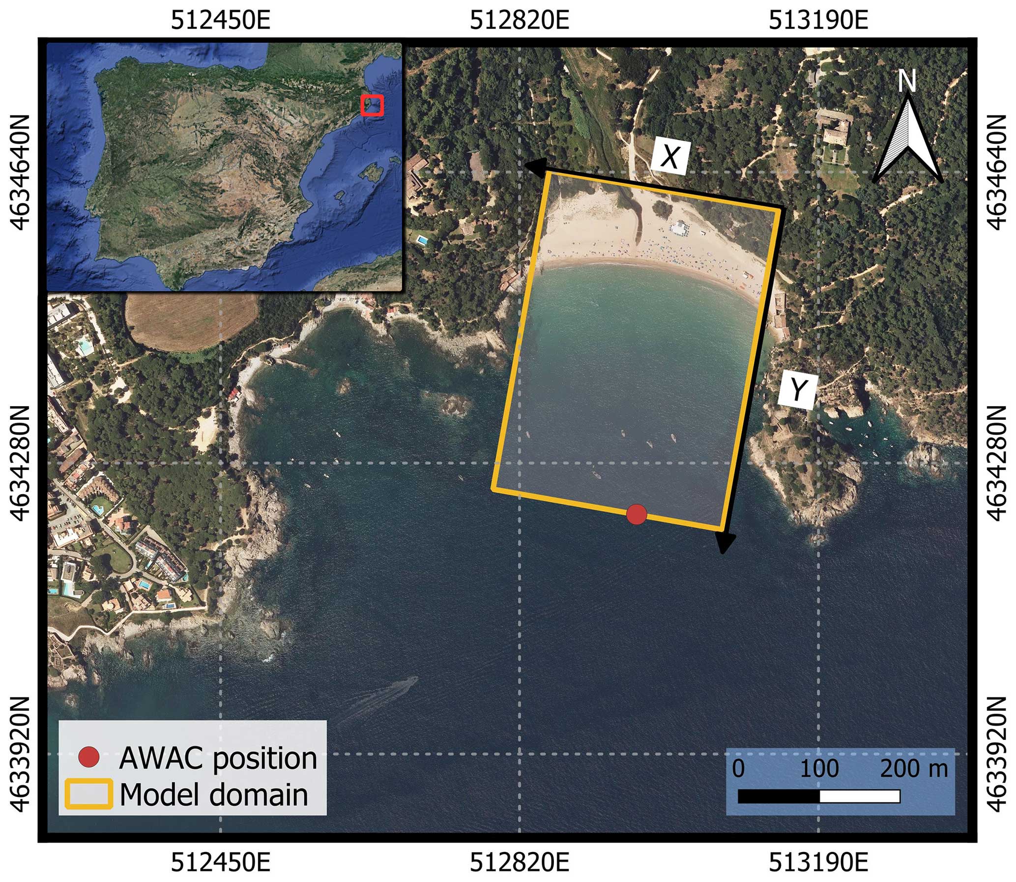
Figure 1Map of the study site showing the domain of the morphodynamic models and the AWAC position. Arrows show the local coordinate system (x,y) used in this study. (Source: © Google Earth, Image from Institut Cartogràfic i Geològic de Catalunya).
The Catalan coast is an area of low-to-intermediate wave energy, where calm periods are dominant during most of the year, especially during spring and summer. Storms, which are usually observed during autumn and winter, are defined here as periods of more than 12 h with significant wave height (Hs) exceeding 1.5 m and an Hs peak exceeding 2.5 m in deep water (Ojeda and Guillén, 2008). The highest-energy events usually reach the Catalan coast from the east, coinciding with the direction of the maximum available fetch (Sánchez-Arcilla et al., 2008). Only southerly and easterly waves can reach Castell beach due to the geometry of the surrounding rocky headlands, and the latter must undergo substantial refraction to arrive at the beach. The astronomical tidal range on the Catalan coast is ∼20 cm (Simarro et al., 2015), while meteorological tides (storm surges) can reach ∼40 cm (return period of 1 year; Toomey et al., 2022).
2.2 Topobathymetric data
Two topobathymetric surveys were conducted on 28 January and 8 July 2020 (Fig. 2). Bathymetry was measured with an R2Sonic® multibeam echo-sounder and a GNSS antenna mounted on a 6 m LOA pneumatic boat, covering the beach embayment extent from approximately 1 to 20 m depth. Echo-sounder measurements were processed using HYPACK® software. An initial automatic filter was applied to eliminate any spike outliers. Adjustments for head, pitch, roll, and heave were automatically applied. A human-eye review of the echo-sounding measurements was also conducted to remove noise sounding. RTK GPS topobathymetric measurements were added to the sounding point cloud for a second review of the data to check elevation matching of the common points between RTK GPS and the echo-sounder. The full data set was then extracted considering cell points of 1 m × 1 m in the post-processed 3D point cloud files. All topobathymetric data referred to the EGM08D595 geoid from the Institut Cartogràfic i Geològic de Catalunya.
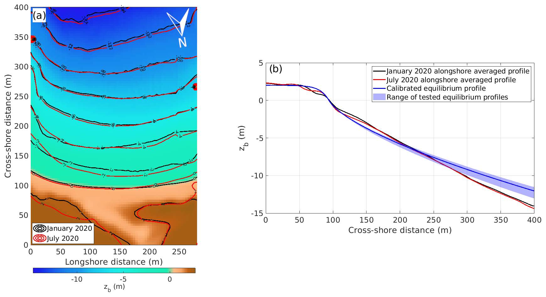
Figure 2Topobathymetric surveys in January and July 2020 within the model domain oriented using the local coordinate system (x,y) shown in Fig. 1 (a) and their alongshore averaged cross-shore profiles (b). Panel (b) also shows the range of tested equilibrium profiles in light blue and the calibrated equilibrium profile in dark blue used in the Q2Dmorfo model. In both panels January is represented in black lines, and July is represented in red lines. The background colours in the left panel correspond to January 2020.
The two measured topobathymetries differed mainly in the shallower area up to 4 m depth, the latest showing a certain overall retreat of the nearshore and shoreline anticlockwise rotation. In both January and July 2020 the beach showed the presence of terraces on their submerged inner zone with a slight decrease in depth of the final one (Fig. 2b). The slope of the swash zone was of approximately βs=0.16, and at greater depths the slope decreased to approximately 0.05. The berm reached a height of about 2 m, and the dry beach displayed the footprint of the creek channel. Most of the observed changes in the dry beach were probably related to the creek position modifications during the 6 months between the two topobathymetries. For further details see Sect. S1 in the Supplement. Note that the 2 months before the first survey were highly energetic, ending with Storm Gloria from 19–26 January 2020 (Amores et al., 2020; Sancho-García et al., 2021; Pérez-Gómez et al., 2021), the strongest storm in at least 30 years that affected the Mediterranean beaches of Spain, coming from the northeast with significant wave heights up to 8 m.
2.3 Wave data
During the 6-month time lapse between the two topobathymetric surveys, hourly wave and sea-level data were measured by a Nortek® acoustic wave and current profiler (hereinafter AWAC) deployed at 14.5 m depth (red circle in Fig. 1). This equipment combines a bottom-mounted upward-facing acoustic Doppler current profiler (ADCP) with a directional wave gauge. The ADCP measures directional currents along the water column, while directional wave parameters are computed using pressure time series, acoustic surface tracking (AST), and surface velocity. The frequency spectrum and other non-directional wave parameters are estimated using these measurements (Pedersen et al., 2007; De Swart et al., 2020). The wave measurement setup used 1200 samples at 1 Hz starting at the beginning of each hour. Raw data were processed by Nortek QuickWave® software, which provided the main wave parameters (non-directional and directional spectrum), surface currents, and mean sea level (Fig. 3).
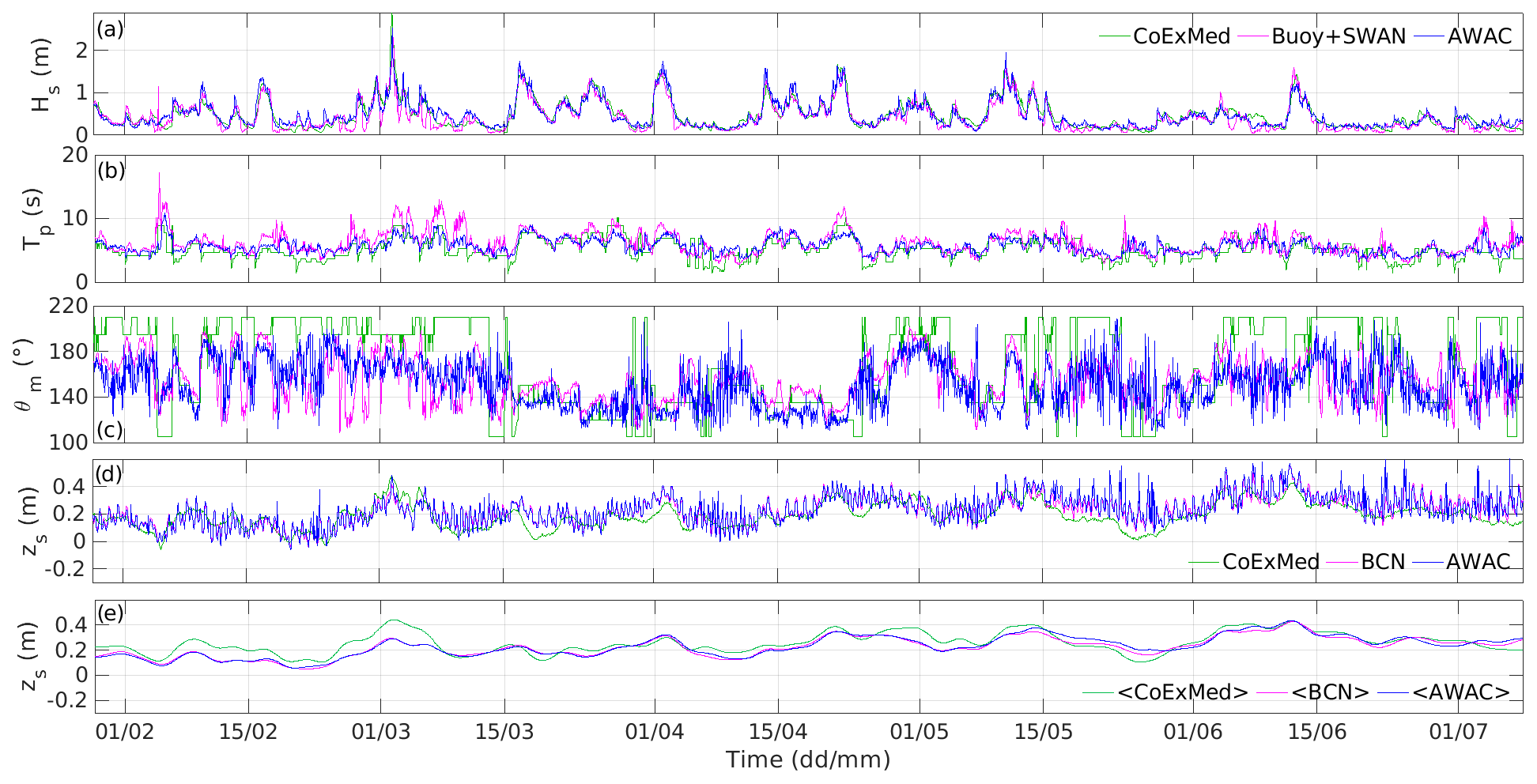
Figure 3Data at the AWAC location of the different forcing sources during the 6-month study period. Time series of significant wave height (Hs) (a), peak period (Tp) (b), and mean wave direction with respect to north (θm) (c) are shown for the three wave data sources. Time series of instantaneous sea-level data from the AWAC, the Barcelona harbour tide gauge, and the CoExMed hindcast are shown (d), as well as the 5 d averaged sea-level data from the latter two sources together with instantaneous sea-level data obtained from CoExMed, also shown in panel (e).
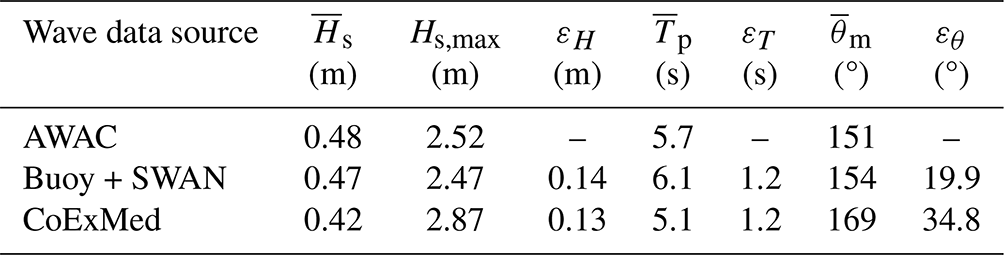
To test the sensitivity of the forcing sources, two other wave sources were used. The first one was obtained by propagating wave conditions measured by the Cap de Begur wave buoy (located at 41.9° N, 3.65° E at a water depth of 1200 m) to the AWAC location (at 14.5 m depth) using the SWAN wave model version 41.31 (Booij et al., 1999; SWAN Team, 2019a, b), following a methodology similar to that of De Swart et al. (2021) (see Sect. S2 for details on the methodology). The second additional wave data were obtained from the CoExMed hindcast, generated using the fully coupled hydrodynamic wave model SCHISM (Zhang et al., 2016) forced by the atmospheric pressure and surface wind from ERA5 (Hersbach et al., 2020) over the Mediterranean Sea (Toomey et al., 2022). The CoExMed data set consists of hourly wave bulk parameters, significant wave height Hs, peak period Tp, and wave peak direction θp spanning the period 1950–2021 with a spatial resolution down to 200 m in coastal areas. Note that the CoExMed wave direction is the peak direction. Nevertheless, the wave peak and mean directions were compared, and there were no significant differences. Thus, from now on, the wave peak direction from CoExMed is referred to as the mean direction in concordance with the two other wave forcing sources. Here, a specific SCHISM simulation was performed to obtain the data at the location of the AWAC. The averaged wave characteristics of the three sources are shown in Table 1.
Table 1Wave characteristics of the different data sources at the AWAC location, with being the mean significant wave height, Hs,max being the maximum significant wave height, being the mean peak period, and being the mean wave direction with respect to north. The root-mean-square error (ε) of the propagated buoy and CoExMed data compared to the AWAC data is also included.
The 6 months of the study were generally not very energetic, but some episodes of medium wave intensity occurred (Fig. 3). In early March, a storm reached the coast from about 160° N with a maximum Hs of 2.5 m, the highest value recorded during the measured period. In fact, waves arrived from the S and SSE a significant percentage (55 %) of the studied time, which is not particularly common on the Catalan coast, where an eastern direction tends to dominate, but the orientation of Castell beach favours the entrance of the southern directions. From mid-March to mid-April, several low-energy storms reached the coast from the east (turning to SE in front of the beach due to refraction) with Hs above 1.5 m. In mid-May and mid-June, two low-energy storms (maximum Hs of 1.5 m) reached the coast from the SSE, but these last 2 months were generally characterized by low-energy wave conditions.
The three wave data sources provided similar values for the significant wave height (Fig. 3a). The peak period obtained from the propagation of the Cap de Begur buoy data using SWAN overestimated the in situ values, whereas the data obtained from CoExMed underestimated them by a similar amount of about 0.5 s (Table 1). The mean directions were better represented by the propagation of buoy data using SWAN than by the CoExMed hindcast. The latter (former) overestimated the angles from the southern waves with a bias of 18° (3°) to the south-southwest and a root-mean-square error (ε) of 35° (20°) (Fig. 3c and Table 1).
2.4 Sea-level data
Three sea-level data sets were used. The first one was measured in situ by the AWAC; the second one was obtained from the Barcelona (BCN) harbour tide gauge (a radar Miros sensor managed by the Puertos del Estado of the Spanish government), which is located ∼100 km from the study area; and the third one was extracted from the CoExMed data set (Fig. 3d and e). The sea level from the AWAC pressure time series was computed assuming hydrostatic conditions above the instrument, assuming constant water temperature and density along the water column, and considering the depth of the instrument deployment and the height from the seabed of the pressure sensor (65 cm). Apart from the wave conditions, the 72-year hindcast by CoExMed also generated the sea-level time series described above. This was done by using the effects of mean sea-level atmospheric pressure, surface winds, waves on total sea surface elevation, and not including the astronomical tide frequencies for the period 1950–2021 and with hourly temporal sampling. Finally, a 5 d running average of the sea-level time series of the three sources was performed in order to test the role of the high-frequency (mostly controlled by tides as defined here) sea-level variability (Fig. 3e). All sea-level data referred to the same geoid as the topobathymetric data in order for all model inputs to refer to the same data set.
The AWAC instrument sank 0.5 m from the initial position where it was deployed during a storm in early March. This affected the sea-level measurements, causing an upward bias in the data recorded since then. In order to fix this problem, the AWAC sea-level data were adjusted to reproduce the monthly trends of the Barcelona harbour tide gauge. Firstly, the two time series were smoothed (to focus on the monthly trends) and subtracted. Then, a hyperbolic function was adjusted to the differences to finally subtract this function to the original AWAC data.
3.1 XBeach model
XBeach is an open-source 2DH morphodynamic model designed to simulate the storm impact on dunes and barrier islands (Roelvink et al., 2009). The model determines the transformation of the directional spectra of offshore waves (which could include groupiness), solves the mean surf-zone hydrodynamics, and then computes the associated sediment transport and the induced seabed evolution at relatively short timescales of days–weeks. A brief description of the equations and parameterizations used within XBeach, especially focusing on sediment transport and bed evolution, is presented in Sect. S3.1, and a full description of the model can be found in the literature (e.g., van Thiel de Vries, 2009; de Vet, 2014; Elsayed and Oumeraci, 2017).
In the present application, the XBeach model version 1.23 was applied to a rectangular domain, localized as shown in Fig. 1, with the cross-shore coordinate rotated 190° with respect to north to adequately represent the Castell beach area and rocky headlands. The rectangular grid had an alongshore extension of 280 m and a cross-shore extension of 400 m. Several grid resolutions were initially tested, and the optimum values were found to be 4 m × 4 m. Smaller resolutions resulted in an overly high computational cost, and larger ones were not accurate enough to describe the shallower parts of the domain. A morphological acceleration factor fmor=10 (Eq. S4) was set to reduce the computational time. Values of 5 and 20 were also tested with no significant changes, in agreement with Lindemer et al. (2010) and McCall et al. (2010). The position where the AWAC was deployed corresponded with the domain offshore limit. Thereby, the wave and sea-level conditions available at the AWAC location (Sect. 2) could be directly applied at the seaward side of the domain. Lateral boundary conditions were set as no-flux conditions for water and sediment. The headlands were simulated in XBeach with 2 m × 2 m non-erodible cells located at the offshore end of each headland (at 344 m and 264 m from the x axis in the east and west, respectively). These cells influence wave propagation from the offshore boundary to the coast, generating the proper wave shadowing and diffraction due to the presence of rocky headlands and avoiding the typical scour effects of placing rectilinear solid walls in this model. The model configuration, parameterizations, and parameters values used are given in Sect. 4.1 and Table 2.
Table 2List of several of the parameter values used in the XBeach model with their default and calibrated values.
3.2 Q2Dmorfo model
Q2Dmorfo is a reduced-complexity coastal morphodynamic model especially designed for large spatiotemporal scales (up to tens of kilometres and decades). Its essential simplification with respect to 2DH models (e.g., XBeach) is that the mean hydrodynamics are not resolved, so the sediment fluxes are computed parametrically from the wave field. On the other hand, in contrast with one-line coastline models, the full topobathymetry is handled by solving the sediment conservation (Eq. S4). Wave transformation is performed over the evolving bathymetry assuming monochromatic waves and geometric optics approximation. Its most important equations are described in Sect. S3.2, and a full description can be found in Arriaga et al. (2017).
Here, a Cartesian coordinate system was used, with the x axis pointing alongshore, the y axis pointing seaward, and the z axis pointing upward. Note that the coordinate axes x–y were rotated with respect to the common model description (see, e.g., Arriaga et al., 2017). The seabed was located at , and the mean sea level was at . The same computational domain of XBeach was used for Q2Dmorfo (Fig. 1) but with a different grid: Δx=5 m, Δy=1 m. The choice of the grid spacing was motivated by the horizontal-length scale of the observed morphological changes in view of previous applications of the model (see, e.g., van den Berg et al., 2012; Arriaga et al., 2017; Falqués et al., 2021). The east and west lateral rocky headlands were represented by two rectilinear solid walls of 344 m and 264 m length, respectively, starting at the x axis. The time step was Δt=1.73 s, which is the largest value that ensures numerical stability. Regarding the sediment flux boundary conditions, no flux was assumed at the landward boundary and at the lateral boundaries (representing the headlands that limit the embayed beach). The offshore boundary conditions were open, represented by a linear extrapolation of the sediment flux. Finally, the wave and sea-level data at the AWAC location (Sect. 2) were directly applied as boundary conditions at the offshore boundary of the domain, as in the XBeach case. At the lateral boundaries, the shadows of the headlands were handled in a parametric way, especially introduced in the model for this application. For every wave angle at the tip of the (waveward) headland, a shadow zone next to the headland was defined by the limiting wave ray. Inside the shadow zone, wave refraction and diffraction were considered parametrically, somehow imitating Sommerfeld's solution (Dean and Dalrymple, 2001). The model parameter values used are described in Sect. 4.2 and Table 3.
Table 3List of several of the parameter values used in the Q2Dmorfo model with their default and calibrated values.
3.3 Metrics for the analysis
Both models were first calibrated using the 6-month data set including two topobathymetries and the wave and tide conditions measured in situ with the AWAC at the embayed Castell beach (Sect. 2). The models were initialized with the January 2020 bathymetry, and the objective was to find the set of parameter values that provided the best model results compared with the observed bathymetry in July 2020.
To assess the performance of time evolution morphodynamic models, the root-mean-square error (ε) and the Brier skill score (BSS) were used (e.g., Sutherland, 2004; Vousdoukas et al., 2011), the latter measuring the error in the model prediction relative to the observed changes (δ):
Here, N corresponds to the number of cells inside the area used to calculate the BSS, Ymodf corresponds to the final model results, Yobsf corresponds to the observed values in July 2020 (ground truth), and Yobsi corresponds to the initial values in January 2020. A BSS of 1 means that the model perfectly reproduces the observed change, whereas a skill value smaller than 0 means that the errors in the model prediction are larger than the observed changes. In van Rijn (2003) a classification was presented to assess qualitatively the BSS values related to morphological changes (e.g., was regarded as “reasonable”, and was called “good”).
In the Q2Dmorfo case, only the BSS of the coastline was computed because, regarding the bathymetry, Q2Dmorfo is intended to resolve just the overall trends but not the details. Since XBeach was developed to simulate surf-zone morphodynamics, the bathymetric BSS was calculated from −3.5 m to 0.5 m to embrace the areas with the most significant bottom changes. In addition, the XBeach coastline BSS was also computed in order to compare it with the Q2Dmorfo one. For each set of parameter values tested during the XBeach calibration procedure, we performed 15 realizations to handle the randomness in the offshore wave groupiness (more details in Sect. 4.1). Then, we computed a mean bathymetry out of these realizations to finally calculate the BSS of this bathymetry and its coastline. Also, our goals in the calibration procedure were to obtain not only accurate but also robust (i.e., reproducible) results. Thereby, the standard deviation σ between the results of the 15 realizations and the corresponding mean (of both the coastline and the bathymetry) was also calculated to evaluate the potential dispersion within realizations. For both models, the optimal set of parameter values was those providing a high value of the BSS, but for the XBeach model a low value of the σ was also required to ensure the robustness and repeatability of the results. To obtain the final result for the optimum parameter setting, 15 more realizations were added to increase robustness.
4.1 XBeach
Applying the XBeach model to the site using the default model settings (those of version 1.23, shown in Table 2) produced the well-known overestimation of erosion (Kombiadou et al., 2021), yielding negative BSS values for both bathymetry and coastline. Model results significantly improved by calibrating the model configuration and parameter set as explained hereafter. The surfbeat mode was selected for this study to simulate the beach response to the incoming waves with a realistic onshore transport in the surf zone minimizing the observed shoreline recession, in agreement with the literature (Rutten et al., 2021; Bae et al., 2022). When this mode is used, XBeach generates wave time series within the spectral wave boundary condition that include wave groupiness, imitating the stochastic nature of a real sea. In this configuration, the choice of the parameter 𝚛𝚊𝚗𝚍𝚘𝚖=1 generates for each simulation a time series of slightly different waves. This affects beach dynamics: in each “particular simulation” the incident wave changes, sediment transport is modified, and the response of the beach differs with exactly the same model configuration. To adequately deal with this randomness in the offshore wave groupiness, many realizations were made to account for the corresponding variability in the beach response. In the calibration phase, 15 realizations for each parameter set were applied, and 15 more were added to obtain the final result for the optimum parameter values (as explained in Sect. 3.3).
Preliminary tests concluded that the effects of the turbulence induced by the wave breaking on the equilibrium sediment concentration, represented by the parameter kb (Eq. S3, Sect. S3.1), had to be computed with the wave_averaged mode. Either using the bore_averaged mode or switching off this parameter increased the unrealistic erosion overestimation of XBeach. The default value of the bed slope parameter (Eq. S5) was used, fsl=0.15 (de Vet, 2014), and the value of the swash zone slope measured in the January 2020 topography was applied, βs=0.16.
The key parameters on cross-shore sediment transport fSk and fAs (Eq. S2), involved in the formulation of wave asymmetry, were calibrated within the range given in Table 2. The calibrated values of the rest of parameters shown in that table were initially used. The values fSk=0.55 and fAs=0.35 provided high bathymetric and coastline BSS values and the lowest possible σ values (Fig. S4). Selected values of fSk and fAs did not yield the highest BSS but provided sufficient accuracy and, at the same time, robustness and reproducibility across the 15 realizations. Lower values led to a decreased BSS due to modelled coastline shifting seaward compared to observed, often resulting in a negative BSS. Larger values underestimated the observed erosion.
Thereafter, the bed friction coefficient n in the Manning formulation for the bottom friction coefficient cf was varied within the typical range for simulating sandy beach bed friction (e.g., Schambach et al., 2018; Passeri et al., 2018; Kombiadou et al., 2021); see Table 2. The value n=0.03 was chosen for giving the highest BSS and the lowest σ (Fig. S5). Lower values of n induced higher erosion rates in the surf zone, while higher values prevented sand mobilization, reducing transport and erosion.
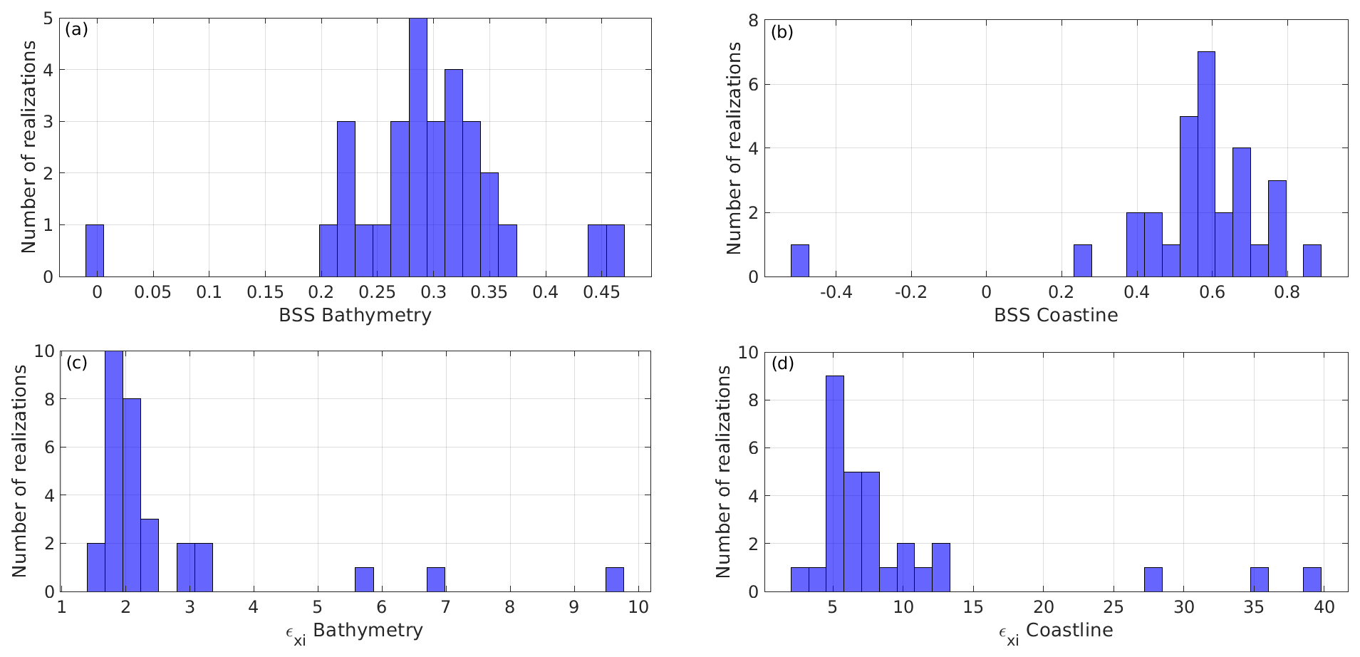
Figure 4a displays the coastlines obtained within the 30 realizations performed for the calibrated case (light blue), showing the low deviation between them, and the computed mean coastline (magenta). The mean coastline and the majority of individual ones show a good performance in relation to the final observed coastline (dark solid line) with low bias values (Fig. 4b). The variability in the results of the BSS and the root-mean-square deviation εxi of the 30 individual realizations for the optimal set of parameters is also illustrated in Fig. 5. Numerous cases with high values of the BSS and low values of εxi were obtained, with a few of them giving low BSS values and a big εxi. These results show that the selected optimal values are accomplished with the principles of robustness and repeatability that were targeted during the calibration procedure.
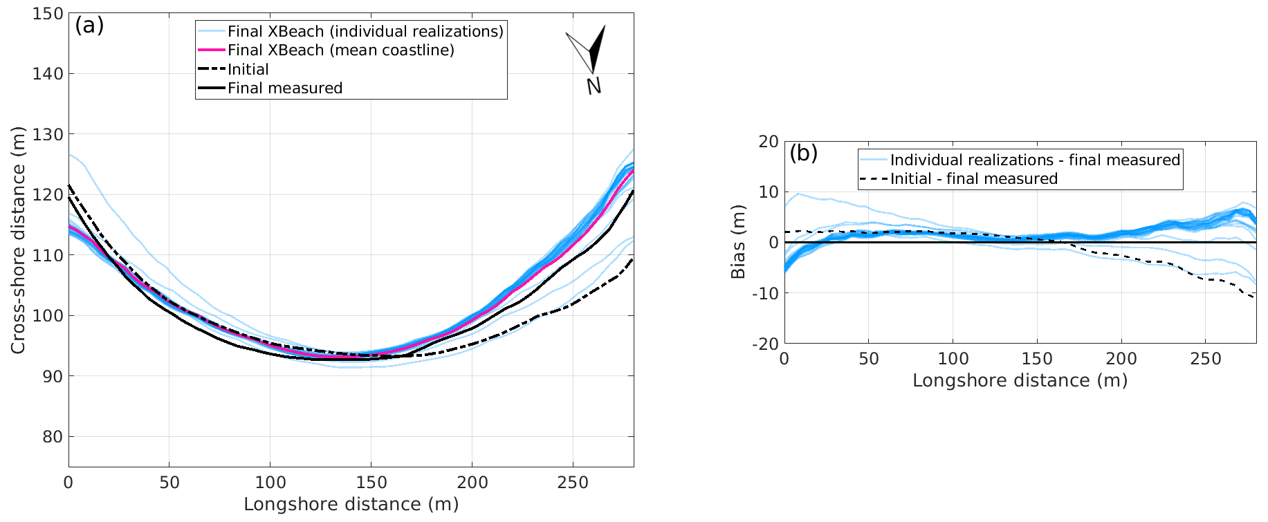
Figure 4Panel (a) represents the measured coastlines in January 2020 (initial, dashed black) and in July 2020 (final, solid black), as well as XBeach-modelled coastlines within the 30 realizations (light blue) and the corresponding mean (magenta). Panel (b) shows the bias between the individual realizations and the final measured coastline (light blue). The bias between the two observed coastlines is represented in dashed black. The calibrated parameter values shown in Table 2 are used.
4.2 Q2Dmorfo
An important difference of Q2Dmorfo with respect to XBeach is that, for the former, an alongshore uniform equilibrium beach profile must be defined. Here, a Dean-shaped equilibrium profile, which depends on two parameters (Eq. S8, Sect. S3.2), was applied. The slope of the swash zone was taken to be equal to the measured one, βs=0.16, and the water depth at 291 m from the shoreline, D1, was a calibration parameter. Its default value (Table 3) was obtained by visually adjusting the Dean profile to the shallower part of the measured bathymetries. The other two important parameters to be varied were those controlling the intensity of the alongshore transport, μ (Eq. S7), and the intensity of the cross-shore transport, ν (Eq. S10). Their default values came from a previous detailed calibration (Ribas et al., 2023). For the r parameter in Eq. (S7), the existing literature (Horikawa, 1988) advises r∼1, and here we examined values ranging [0,3]. Preliminary simulations proved that the best choice was r=2.
The 196 combinations of parameter values tested during the calibration and the final calibrated values are also shown in Table 3. The best model performance (highest BSS) was obtained for μ=0.019 , ν=0.025, and D1=11.7 m. As can be seen in Fig. S6, the BSS was very sensitive to D1, which controls the overall progradation/retreat of the shoreline, with low (high) values of D1 producing shoreline retreat (progradation). For example, given a cross-shore bathymetric beach profile and a D1 that is small enough, the equilibrium profile is shallower than the actual profile. In such a situation, the actual profile (steeper than the equilibrium one) experiences an offshore gravitational transport that is more intense than the onshore wave-driven transport. Since the resulting sediment transport is seaward, the shoreline retreats, and the actual profile tends to the shallower equilibrium one. The contrary occurs for a large enough D1.
The μ parameter had less influence, as can be seen from the overall vertical trend in the isolines in Fig. S6. This was probably due to the long period (6 months) studied. During a particular storm, the curved shoreline of the embayed beach would tend to become locally perpendicular to the wave incidence direction (at the breaking line). Whether this orientation is reached or not depends on a balance between the intensity of the sediment transport (μ) and the duration of the storm. If the duration is long enough, the final shoreline orientation will be roughly independent of μ. Here, given the long time period of the simulation, it turns out that the shoreline tended to a (curvilinear) shape that was mainly determined by the resulting mean wave direction, and the intensity of the longshore transport just influenced how quickly this equilibrium was reached. It similarly occurred with the cross-shore transport, with the parameter ν (which controls the timescale of the tendency to equilibrium) having even less influence than μ. In the present long simulations, the final cross-shore bathymetric shape was mainly controlled by the prescribed equilibrium profile, being quite insensitive to the intensity of the transport (ν).
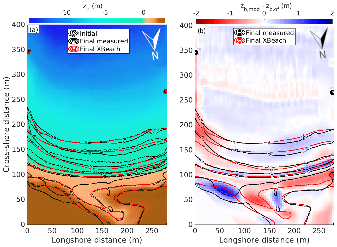
Figure 6(a) Comparison between the final topobathymetry modelled by XBeach (solid red contours), the final observed one in July 2020 (solid black contours), and the initial one of January 2020 (dashed black contours and background colours). (b) Difference between the final modelled and observed topobathymetries (background colours), with the modelled and observed topobathymetric contours in red and black, respectively. The calibrated parameter values are used (Table 2), with the wave and sea level measured by the AWAC.
5.1 Morphodynamic evolution using in situ data
The calibration of the two models allowed a fairly accurate simulation of the observed beach morphology after the 6-month study period (Table 4). The BSS obtained for the XBeach optimum result was 0.38 for the bathymetry and 0.74 for the coastline (computed from the averaged bathymetry of 30 realizations). In the case of the Q2Dmorfo, the optimum simulation gave a coastline BSS of 0.79. The bathymetric BSS (not used in the Q2Dmorfo calibration) was negative (−0.44). According to van Rijn (2003), the accuracy of the XBeach bathymetry simulation could be regarded as “reasonable”, and the coastline simulation in both models would be “good” (close to “excellent”).
Table 4Root-mean-square error (ϵ) and Brier skill score (BSS) from XBeach (XB) and Q2Dmorfo (Q2D) using the different forcing sources, where 〈〉 means a 5 d running average. The calibrated parameter settings (Tables 2 and 3) were used.
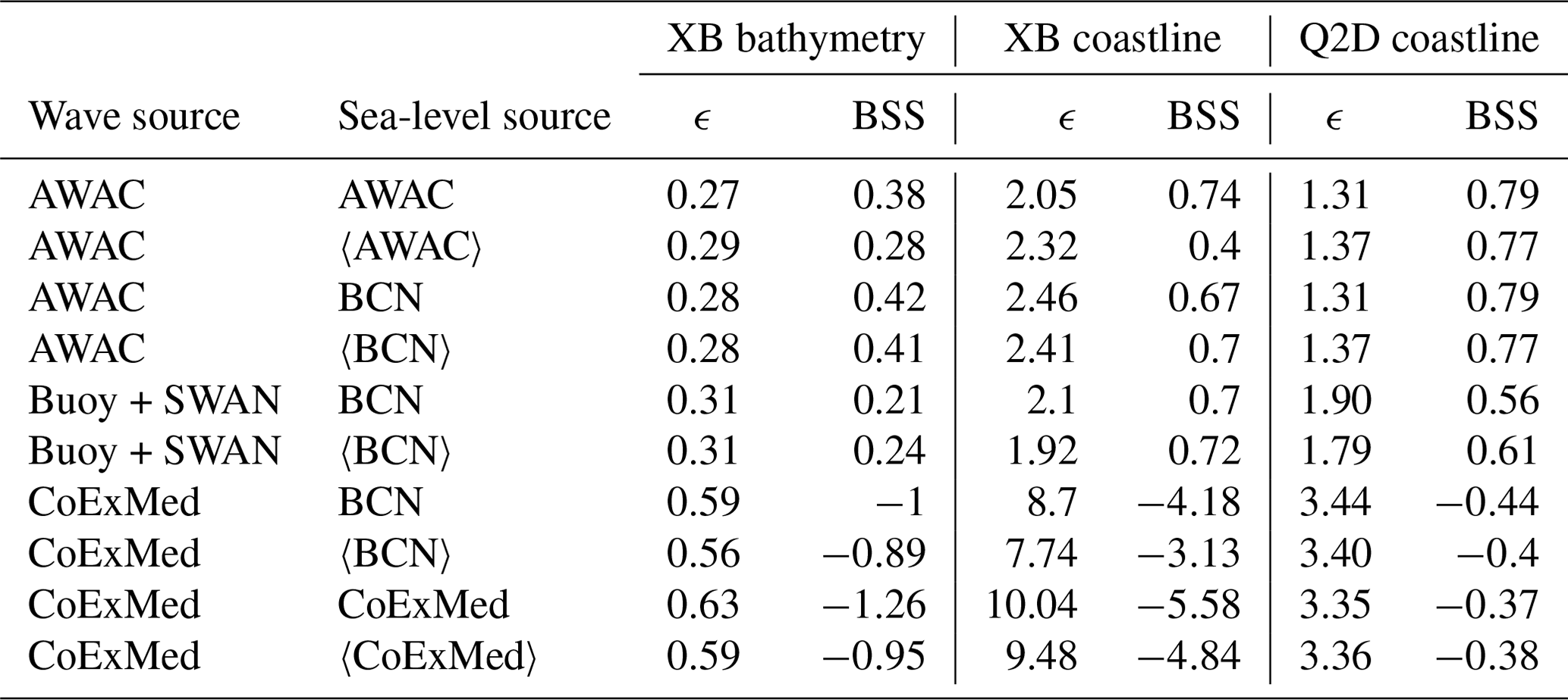
The XBeach mean bathymetry (computed from the 30 realizations) showed a good resemblance to the final bathymetry observed in July 2020 (Fig. 6). The model was able to simulate the observed surf-zone retreat from the shoreline up to 2 m depth quite accurately, but it predicted hardly any changes at larger depths. The Q2Dmorfo model was also good at modelling the coastline, but it was less precise in describing the surf-zone bathymetry (Fig. 7; isobaths of −1 and −2 m). This is coherent with the fact that it is not designed to simulate the details of the bathymetric evolution (Sect. 3.2). However, the Q2Dmorfo bathymetric contours tended to qualitatively follow the observed changes in the −3 and −4 isobaths, except at the eastern side. In fact, a localized strong erosion (compared to observations) was produced by both models next to the eastern headland at depths greater than 2 m (Figs. 6b and 7b). Moreover, the models did not properly resolve the evolution of the dry part of the beach, as the processes driving it were not included (role of the creek and aeolian transport).
Figure 7(a) Comparison between the final topobathymetry modelled by Q2Dmorfo (red solid contours), the final observed one in July 2020 (solid black contours), and the initial one of January 2020 (dashed black contours and background colours). (b) Difference between the final modelled and observed topobathymetries (background colours), with the modelled and observed topobathymetric contours in red and black, respectively. The calibrated parameter values are used (Table 3), with the wave and sea level measured by the AWAC.
Both models accurately simulated the observed anticlockwise shoreline rotation (Fig. 8), consistent with an overall western-directed sediment transport produced by the SE- and SSE-dominant wave incidence directions. XBeach tended to overestimate shoreline accretion during the 6-month study period, except at the easternmost zone. The shoreline simulated by Q2Dmorfo showed an overly large retreat on the central part, but on the western stretch of beach, which is the most exposed to the eastern-dominant waves and where more shoreline variability is observed, the adjustment between model and observation was very good. The westernmost and easternmost parts of the Q2Dmorfo-modelled coastline experienced too much erosion, again due to the idealizations in modelling wave propagation with the rocky headlands.
5.2 Morphodynamic evolution using other forcing sources
To test the sensitivity of the modelled beach response to using other forcing sources, different combinations of the wave and sea-level sources (described in Sect. 2) were applied using the parameters determined by the calibration of the models. Firstly, the AWAC wave data were combined with the 5 d averaged sea-level series measured by the same instrument and with the Barcelona (BCN) harbour gauge instantaneous and averaged series. Secondly, the wave data from the Cap de Begur buoy propagated by SWAN were combined with the instantaneous and the 5 d averaged sea-level series from the Barcelona harbour tide gauge. Finally, the wave data computed by CoExMed were combined with the instantaneous and averaged sea-level data from the Barcelona harbour gauge and with the instantaneous and averaged sea level from the CoExMed hindcast (see Table 4 for a list of combinations of the forcing sources). The parameter setting resulting from the calibration (Tables 2 and 3) was used in both models. In order to add more robustness to the final results, a total of 30 realizations were carried out in XBeach for each combination of forcing sources tested.
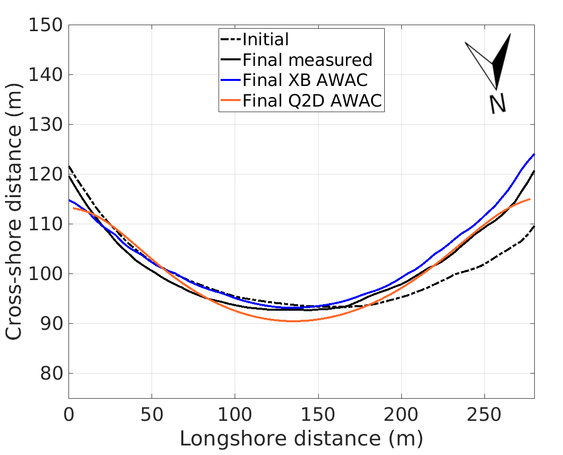
Table 4 presents the BSS results obtained by applying all the combinations of forcing sources in the two models. The simulations with both models using wave data propagated with SWAN from the Cap de Begur buoy gave a beach response similar to when using AWAC data but with a slight skill decrease. Essentially, the observed anticlockwise rotation of the coastline was captured (Fig. 9). This is logical, since the mean wave characteristics were similar to those of the AWAC wave series (Table 1). However, using the third source of wave forcing, the one from the CoExMed hindcast, significantly worsened the skill, obtaining negative BSS values in both models. The reason is that the CoExMed waves had angles biased towards the SW (Fig. 3 and Table 1). Then, both models underestimated the anticlockwise rotation of the beach (Fig. 9), since there was less western-directed sediment transport using this wave source.
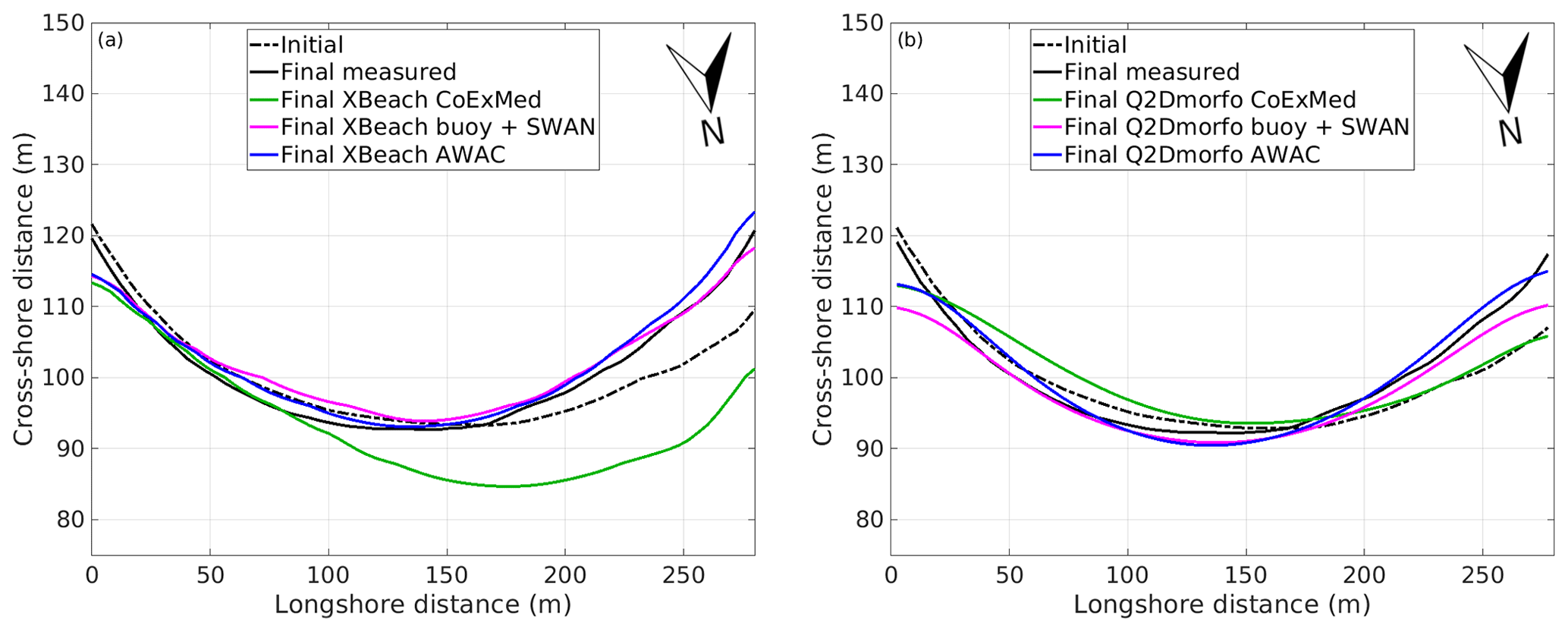
Figure 9Final modelled coastlines using the three different wave forcing sources in the XBeach model (a) and Q2Dmorfo model (b). In this figure, the sea level measured by the AWAC was selected for the AWAC wave source, the sea level from the Barcelona harbour was used with the buoy plus SWAN wave data, and the CoExMed sea level was chosen for the CoExMed wave data. The calibrated model parameter settings (Tables 2 and 3) are used.
There were no significant variations between the results obtained by the models using different sea-level sources when the wave source was maintained (Table 4). Also, the 5 d averaged sea-level series in general gave a result similar to the corresponding instantaneous sea-level one. Exceptionally, using the AWAC-averaged sea-level worsened the XBeach BSS values obtained using the AWAC instantaneous series (decreasing the bathymetric and coastline BSS by ∼30 % and ∼50 %, respectively), but the simulation skills remained reasonable. No explanation has been found for the BSS worsening that occurs in this case.
To examine the modelled evolution of beach morphology in more detail, we defined a modified BSS (called BSS*(t) from now on) to account for time dependence. To do so, we applied Eq. (1) but with Yobsf being the result of the numerical run forced with in situ AWAC measurements at every time step. In other words, the latter simulation is defined as the ground truth (or as the benchmark simulation), since it is the closest to the real changes (and used to calibrate the models). The advantage of this new metric is that it allows us to evaluate the impact of the use of different forcing sources compared to the use of in situ observations (Fig. 10f–h).
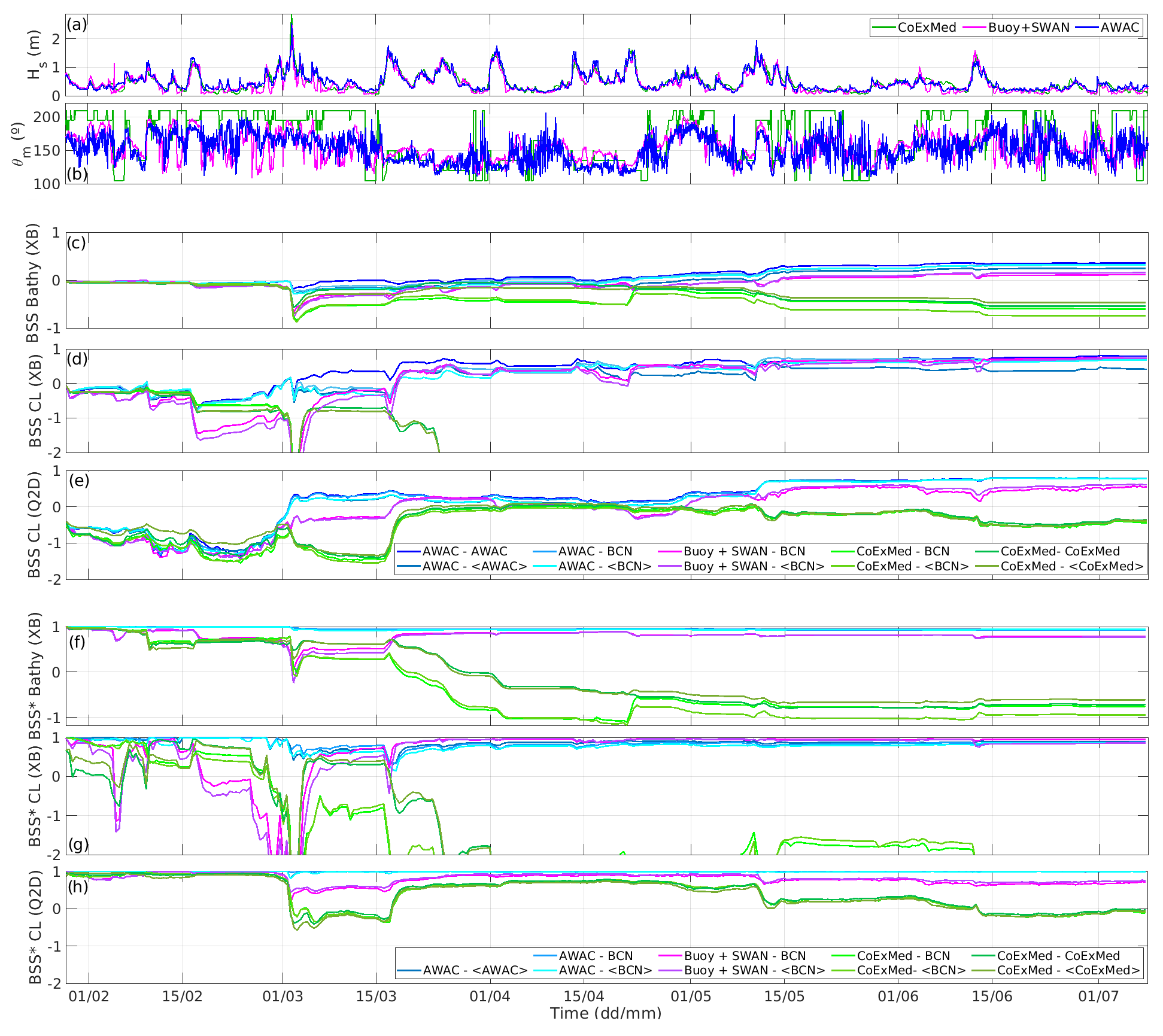
Figure 10Time evolution of the BSS(t) during the 6-month study period, calculated with Eq. (1), using the time-varying XBeach-modelled bathymetries (c), XBeach coastlines (d), Q2Dmorfo coastlines (e), and the corresponding final measurements as ground truth, for all the combinations of wave and sea-level forcing sources. Also, the time evolution of the BSS*(t) during the 6-month study period, calculated with the instantaneous bathymetry and coastline from the simulation forced with AWAC data as ground truth and using the time-varying XBeach-modelled bathymetries (f), XBeach coastlines (g), and Q2Dmorfo coastlines (e), for all the combinations of wave and sea-level forcing sources. The time evolution of Hs (a) and θm (b) for the three wave forcing sources is also shown.
In both models, a similar morphodynamic response was observed with all the forcing sources during the first month up to the storm in early March (the most energetic event of the entire study period, coming from the south). This strongest storm had a smaller effect when the AWAC source was used than when it was simulated using the other wave forcing sources. A pronounced decrease in the BSS and BSS* was observed in both models, especially in those simulations using the CoExMed wave data. After this storm, there was a 15 d period of calm conditions with no major changes until another energetic period of 1 month occurred, characterized by waves coming from the southeast. In the XBeach model, the BSS and BSS* values increased in all simulations except for those using the CoExMed data. The Q2Dmorfo simulations during that episode tended to exhibit similar behaviour for all combinations of forcing sources, obtaining increased values of the BSS and BSS*. During the last 2 months, a combination of calm and moderate conditions reached the beach, with waves alternating between the south and southeastern directions. These conditions affected the beach similarly in both models, with a generalized decrease in the BSS and BSS* when the CoExMed data were used. The behaviour obtained when the data propagated from the buoy were used was similar to that of the in situ data.
6.1 Optimum model configuration and parameter values
Simulating the morphodynamic beach response of Castell beach over a 6-month study period using XBeach was a significant challenge because this model is typically applied to shorter timescales, from days to weeks. Using the surfbeat mode, enabling the random mode (𝚛𝚊𝚗𝚍𝚘𝚖=1), and performing many realizations (15–30) of each simulation (as described in Sect. 3.1) allowed us to reproduce the uncertainty and variability in real stochastic wave climates within XBeach simulations. This resulted in more reliable and realistic outcomes, giving significantly high values of the BSS in one of the few successful applications of XBeach to a 6-month period. The implemented methodology is in line with that of Rutten et al. (2021), who also demonstrated the importance of including the wave time series randomness in XBeach simulations to accurately model bed evolution response, particularly in the complex and dynamic nearshore zone. This is an important learning for future XBeach studies that intend to simulate time periods longer than a week or so. The approach followed in the present study was highly time-consuming and involved extracting the mean bathymetry and its shoreline from the 15–30 realizations for each parameter setting and for each hydrodynamic forcing source combination. Thereby, it required a long and iterative calibration procedure to finally find the optimal parameter values.
In agreement with our results, previous studies also showed that increasing the wave skewness and asymmetry (facSk and facAs factors) leads to an increase in the onshore sediment transport and mitigates the well-known issue of erosion overestimation in XBeach simulations. For instance, Schambach et al. (2018) demonstrated that raising these factor values above their default setting (0.1) resulted in an improved performance, with an optimal value of 0.3 for both parameters in the analysis of cross-shore profile evolution during a storm on an open beach in Rhode Island. Similarly, Kombiadou et al. (2021) used higher values (0.65–0.75) to reduce the erosion overestimation in cross-shore sections during storm periods in a 2-month simulation on Faro Beach, an Atlantic open beach in southern Portugal. Furthermore, Sanuy and Jiménez (2019) conducted an extended calibration of these parameters to simulate a stormy period on an open beach on the Catalan coast, identifying an optimal value of 0.6 for each factor. Remarkably, the optimum values obtained in this study (𝚏𝚊𝚌𝚂𝚔=0.55 and 𝚏𝚊𝚌𝙰𝚜=0.35) are consistent with those reported previously. In fact, as shown in Fig. S4, positive values of the BSS (dark red) were only obtained for high values of these two parameters. Note that, since the first topobathymetry in January 2020 was measured a few days after Storm Gloria, which was the strongest in at least 30 years and probably induced a significant beach erosion, such large values of facAs and facSk were probably needed to compensate for the potential storm-induced erosion with an increasing onshore transport. Using the wave_averaged mode on the turb parameter showed good results, mitigating the beach erosion observed when the default mode (bore_averaged) was used. Previous studies such as Kombiadou et al. (2021) also used this mode, obtaining good outcomes with a realistic erosion trend compared to the observed data. The simulations to assess the optimum value of the Manning bed friction coefficient (n=0.03 ; Fig. S5) revealed its influence on the model performance. Similar findings were presented in Melito et al. (2022), where the importance of this parameter was also highlighted, emphasizing the requirement of increasing its default value (from 0.01 to 0.045 ).
The Q2Dmorfo skill in modelling coastline behaviour is also noteworthy, bearing in mind the number of idealizations behind this model. This positive result proves that the present model version is appropriate for embayed beaches. In fact, when the calibrated simulation was repeated switching off the recently included effect of the headland's shadow on the waves (described in Sect. 3.2), the model results became completely unrealistic compared with the observations. The most critical Q2Dmorfo parameter was D1, controlling the overall slope of the equilibrium profile. The obtained best value (D1=11.7 m at 293 m from the shoreline) gave an equilibrium profile that was consistent with the overall trend in the first 6 m depth of both observed bathymetries. In other words, the equilibrium profile selected by the calibration follows the observed bathymetries within the upper shoreface, the most active area. In contrast, this equilibrium profile deviates from the observed bathymetry in deeper water. However, this has no effect on the morphodynamic evolution, since wave stirring and sediment transport are insignificant there. Interestingly, the selected equilibrium profile somewhat better fits the final bathymetry (see the dashed line in Fig. 2b). This is likely due to the fact that the initial one was taken just after Storm Gloria and that the beach was probably a bit far from equilibrium at that time. The optimum values of the sediment transport parameters at Castell beach (μ=0.019 and ν=0.025) were half the ones obtained in the detailed Q2Dmorfo validation with data from the sand engine in the Netherlands (Arriaga et al., 2017; Ribas et al., 2023). This is not surprising because the grain size of the study site is 50 % larger than the one at the Dutch coast, and the water velocities are smaller due to the embayment influence, with both factors resulting in lower sediment transport rates. Note that the value of the K parameter in the CERC constant corresponding to μ=0.019 is K=0.065, smaller than the lowest values found in the literature. However, there is a high uncertainty regarding the K value (Arriaga et al., 2017), and the present detailed study is a good opportunity to assess it on embayed beaches, which had been scarcely modelled before. To confirm the article findings, the calibration procedure of Q2Dmorfo was also pursued using CoExMed forcing for both waves and sea level. The obtained optimum parameter values were the same as for the AWAC-forcing calibration, but the skill was negative, . Interestingly, by playing within a wide range of D1, μ, and ν parameters, there was no way to improve this skill. This is important, since it shows that the good skill obtained when forcing with the AWAC is not an artefact of the parameter selection but has to do with the physics included in the model.
The calibration results of both models were influenced by the use of only the initial and final topobathymetries. The absence of interim observations during the 6-month period inhibited validating the models' performance during the simulation time lapse. When assessing calibration results, it must also be considered that the initial beach was in an exceptionally erosive state, such that the performed calibration could be biased towards accretive conditions. Nevertheless, the calibration was essential to reduce the root-mean-square error and to obtain a positive BSS for both models compared to default settings and parameter values. After calibration in XBeach, the ϵ of the shoreline and bathymetry was reduced by 85 % and 67 %, respectively, while in Q2Dmorfo the shoreline ε was reduced by 63 %.
6.2 Comparison between the performance of the two models
Despite both models providing a good prediction of the beach evolution during the 6-month study period, discrepancies were observed when comparing their results to the final observed topobathymetry. Both models presented a remarkable eroded area at the easternmost part of the beach at depths of approximately 3–4 m (Figs. 6b and 7b). A probable explanation for this issue could be the oversimplifications employed by both models to represent the real behaviour of waves as they propagate towards the coast from the southeast and interact with the headland. This is much more noticeable in the Q2Dmorfo case, which shows larger model–data differences that extend to deeper waters (Fig. 7b) and happens because this model is significantly more idealized (see Sect. 3.2). In particular, the simplifications affecting the easternmost side are (i) assuming monochromatic waves that then form a sharp shadow zone, (ii) neglecting the role of the surf-zone currents (and bars) that might play a role near the headland, and, most importantly, (iii) using a simplified cross-shore sediment transport based on an imposed alongshore uniform equilibrium profile (see Sect. 4.2) whilst measured bathymetries are shallower in this easternmost area compared with the rest of the beach (as can be seen in the first 40 alongshore metres in Fig. 7a). These idealizations are an important factor in explaining why the bathymetric BSS in Q2Dmorfo always had negative values. In fact, when the bathymetric BSS is calculated in both models deleting the first 40 m on the eastern part of the beach, the values obtained significantly increase (∼200 % in Q2Dmorfo and ∼40 % in XBeach). In Q2Dmorfo, the BSS obtained reached 0.43, whereas XBeach obtained a BSS of 0.52. Additionally, the complexity of the real shape of the rocky headland, which is represented by a simple rectilinear wall in the Q2Dmorfo model and by a 2×2 non-erodible pillar in XBeach, also contributes to the differences at the easternmost side in both models. Finally, since neither model simulates the dry beach, there were big differences in that region between model results and the topobathymetry of July 2020. Processes not included in the models, such as the movement of the stream mouth, its discharge during rainy periods, and the aeolian action, contribute to these differences.
To assess how the models differed in their morphodynamic response throughout the 6 months, the bed-level and shoreline variabilities were calculated in the two simulations forced by the in situ measurements from the AWAC (Fig. 11). The alongshore-averaged shoreline variability was defined as
with Δt=12 h. A similar expression was used for the surface-averaged bed-level variability, 〈Δzb(t)〉 (involving and the integral being in x and y). An important contrast was observed between the models in the bed-level variability during the first month, where Q2Dmorfo showed significantly greater changes than XBeach. This strong Q2Dmorfo variability was induced by the model tendency to reach the same imposed equilibrium profile all along the beach and, in particular, at the easternmost section. As we just mentioned, the measured bathymetries clearly showed shallower-than-average profiles in the easternmost 40 m along the beach. Thereby, the initial storms produced fast and substantial changes in the modelled easternmost area to reach the equilibrium shape. Throughout the next 2 months, which included the strongest storm and subsequent eastern-dominated wave conditions, both models showed similar bed-level variability, with significant changes during the high-energy events and minimal changes during calm periods. Along the last 2.5 months, the bed-level changes in Q2Dmorfo were again larger than those of XBeach, particularly during storms. Regarding the shoreline variability, both models presented a similar behaviour during the 6-month period (Fig. 11d), but XBeach generally produced higher changes than Q2Dmorfo; i.e., the shoreline reacted more quickly to storms in XBeach than in Q2Dmorfo. The probable reason is that the differences between the idealized cross-shore transport in Q2Dmorfo and the more realistic description by XBeach become more pronounced in very shallow water. Finally, it is interesting to note that, despite Q2Dmorfo coastline responding less to individual storms than XBeach coastline, it eventually reaches the same values in the medium term.
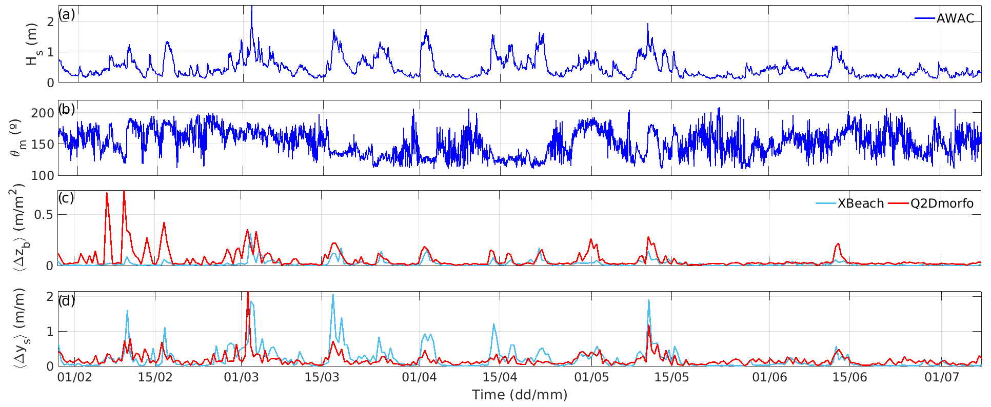
Figure 11Differences in the instantaneous modelled bed-level variability during the 6-month study period, when both models were forced with the AWAC data. The time evolution of Hs (a), θm (b), bed-level variability (〈Δzb(t)〉) (c), and shoreline variability (〈Δys(t)〉) (d) for the two models is shown.
The computational times for both models differ substantially. Performing a 6-month simulation using the described XBeach setup (Sect. 3.1) lasts ∼12 h, parallelized in 10 computational processors. Taking into account the 30 realizations to deal with the random effect, it adds up to ∼3600 h of computational time. Note that using an irregular grid could decrease the number of modelled points in XBeach and thereby reduce the computational time. In contrast, each simulation performed by the reduced-complexity Q2Dmorfo model, with the setup described in Sect. 3.2, lasts ∼8 h, using a single processor. Thereby, the Q2Dmorfo model is about 500 times faster than XBeach, making the former more adequate for long-term modelling.
6.3 Implications of the assessed role of the forcing sources
The results obtained using the different wave and sea-level forcing sources emphasize the importance of having a good description of the wave mean direction (Sect. 5.2), particularly for simulating the morphodynamic response of an embayed beach such as Castell beach. The simulations using CoExMed wave data, which contain a bias in wave angle (Table 1), could not reproduce the observed rotation of the shoreline during the study period (Fig. 9). This effect was magnified when the XBeach model was used, as it resolves more processes compared to the more simplified approach of Q2Dmorfo and is then more sensitive to the wave conditions. The BSS(t) using the various forcing sources did not differ much during the first month (Fig. 10). However, the early-March storm had varying effects on the beach morphology depending on the wave forcing source used. When the waves from the AWAC were used, the coastline BSS increased during the storm, especially for Q2Dmorfo, meaning that the beach evolved towards its final configuration, while the XBeach bathymetry BSS slightly decreased. The wave conditions obtained by propagating the buoy data with SWAN produced a modest shoreline BSS increase with Q2Dmorfo and a decrease for XBeach. However, the BSS converged with that corresponding to the AWAC data forcing during the following storm (showing high BSS and BSS* values at the end of March; see Fig. 10). At the end of the study period, a beach response comparable to that of AWAC simulation was also obtained (Fig. 9), providing only slightly smaller values of the BSS and BSS*. The results obtained with the CoExMed wave data showed the worst behaviour, particularly after the early-March storm, which eroded the beach more than when the other forcing sources were used. The BSS and BSS* never converged back to the values of the AWAC simulation, and at the end of the study period they were always negative. This indicates that, when forced with CoExMed wave data, the beach was not able to recover from the erosion suffered during the energetic episode and could not rotate properly during the rest of the time period.
To understand to what extent this early-March storm was the turning point that led to significant differences between the results obtained using the CoExMed wave conditions, two additional simulations were conducted. Firstly, the modelled bathymetry from the simulation forced with AWAC data (both waves and sea level) in both models was extracted on 15 March, i.e., about a week after the storm, to allow the XBeach bathymetry to stabilize (this model typically produces numerical noise during storms). These bathymetries were then used as initial conditions to simulate the remaining 4-month period using the CoExMed data forcing. The same procedure was also applied but reversing AWAC and CoExMed input data. To compare the results and get further insights into the role of the forcing sources, the BSS* metric defined in Sect. 5.2 was again evaluated for these two additional simulations (Fig. 12). The original run forced with CoExMed data during the 6 months is also shown for comparison. Note that the BSS* metric uses the simulations with 6 months of AWAC data as ground truth (hence assuming it is the most realistic) so that the BSS* quantifies how a simulation with another forcing source diverges from the one forced by in situ data.
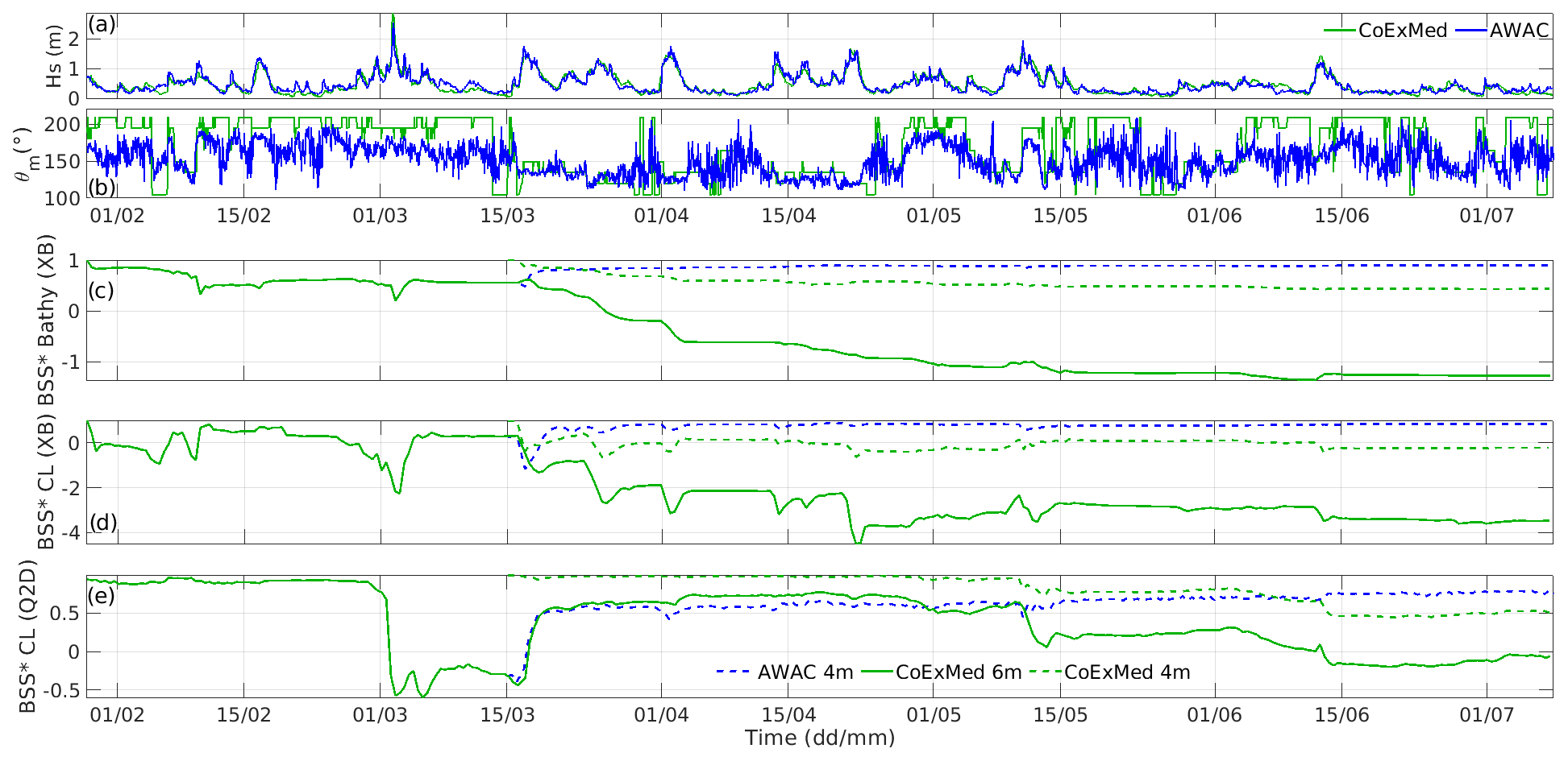
Figure 12Time evolution of the cross-simulation BSS*, calculated with the instantaneous bathymetry and coastline from the simulation forced by AWAC data as ground truth and using the time varying XBeach-modelled bathymetries (c), XBeach coastlines (d), and Q2Dmorfo coastlines (e). The time evolution of Hs (a) and θm (b) for the two wave forcing sources is also shown.
Despite starting with a more eroded bathymetry caused by the CoExMed data of the early-March storm, when we subsequently applied the AWAC data the beach was able to recover and simulate the observed final shoreline rotation in the two models (see the dashed blue lines in Fig. 12c–e, with the final BSS* close to 1). This can be compared to the 6-month simulations forced with AWAC data that correspond to throughout the whole period. In contrast, when the more realistic bathymetry obtained on 15 March with the AWAC forcing was subsequently simulated with the CoExMed data for the remaining 4 months, the errors in the latter source kept producing accumulated differences in the modelled morphology and gave worse final values of the BSS* (dashed green lines in Fig. 12c–e). However, results were better than those obtained when the CoExMed data were applied for the whole 6 months (solid green lines). This indicates that the obtained discrepancies when the CoExMed data source was used are attributable partially to the early-March storm and partially to the rest of the study period. This highlights the importance of having accurate wave data series not only during the storms but also during the rest of the time. On the other hand, our results also indicate that if a wrong data source is used for a short period (i.e., in our case, 2 months) but a more accurate data source is applied afterwards, the morphodynamic model simulations can partially recover their reliability.
The most important implication of this study is that using different wave data sources critically modified the outcome of the morphological simulation. In particular, the known errors in wave direction of existing wave hindcasts of the Spanish Mediterranean coast (shown in Fig. 3 for the CoExMed hindcast and in De Swart et al., 2021, for other existing hindcasts) can produce completely unrealistic morphological simulations. Using the hindcast for simulating the 6-month evolution lead to an ∼314 % increase in error in XBeach and an ∼81 % increase error in Q2Dmorfo compared to using the data propagated from the buoy. This might be especially important at embayed beaches where the waves interact with the structures that limit them and the wave direction is modified due to all the intrinsic propagation processes. Our recommendation for long-term studies is to use the nearest wave buoy and carefully propagate to the site the measured conditions during the study period (see De Swart et al., 2021, and the Supplement for more details on the proposed methodology). However, buoy data contain gaps that are often filled in with hindcast data. The above discussion about the results obtained in the present study when combining these two types of wave source conditions (Fig. 12) underlines that a wrong result produced by errors in a wave data source during time periods of the order of 1–2 months can be compensated for if a correct data source is subsequently applied. An alternative to improve the hindcast data accuracy, and thus the results obtained, could be a previous calibration or a bias correction of the hindcast wave direction. Also, long-term hindcasts can be very useful to fill in the wave buoy gaps with more sophisticated data imputation techniques. In any case, since these results could be site-dependent, it is advisable to perform tests on the sensitivity of morphodynamic modelling to the forcing conditions such as the one presented here before performing long-term studies.
The effect of the choice of sea-level data source was much less important than that of the wave source (Table 4). For example, by comparing the instantaneous data series and the 5 d filtered data series in the 6-month study period, no significant changes were observed (with the only exception mentioned in Sect. 5). This could be attributed to the fact that Castell beach has a very small tidal range, thereby the differences between the instantaneous and the filtered data series were not substantial enough to result in significant changes in the beach response. The implication of the minor influence of the chosen sea-level data source is that different available long-term sea-level data sets can be used when simulating the long-term beach morphological evolution, including tidal gauges located in harbours at distances from the beach of the order of 100 km (such as the Barcelona harbour gauge at the present site). In any case, the choice of sea-level source could be more influential in beaches with a larger tidal range.
The morphodynamic evolution of the embayed beach of Castell (northwestern Mediterranean Sea) during 6 months has been successfully reproduced using two different morphodynamic models, the 2DH XBeach and the reduced-complexity Q2Dmorfo. Remarkably, despite the fact that XBeach was designed to specially simulate storm episodes, very realistic outcomes compared with observations have been obtained in the present longer-term simulations after calibrating it with in situ data. The calibration process was essential, since it reduced the errors by 65 %–85 % compared with the default setting. The following ingredients are essential to avoid erosion overestimation in such types of medium-term XBeach simulations: including the randomness of wave groupiness present in real beaches, performing tens of realizations to account for such randomness, and selecting appropriate values of the cross-shore sediment transport and bed friction parameters. It is important to note that the topobathymetry obtained in January 2020 (used as the initial bathymetry for the models) was obtained a few days after Storm Gloria. It probably affected the beach morphology, which had to recover at the beginning of the study period. This could be one of the main reasons for the high values of the cross-shore transport parameters obtained in the XBeach calibration. Moreover, even though the Q2Dmorfo model is significantly simpler because it was designed to simulate the shoreline evolution over decadal temporal scales, and despite the fact that it does not respond accurately to individual events, it provided excellent results during the 6-month period after calibration. Therefore, this confirms that the model is appropriate to simulate the seasonal morphodynamic evolution of embayed beaches, with a significant reduction in computational cost compared to the more complex XBeach model, even though it only simulates the coastline evolution well.
The choice of the wave forcing source can significantly affect the accuracy and reliability of the results of both types of models. The effect is stronger in XBeach because it includes more physical processes and simulates stronger changes, such as those produced by individual storms. In both models, the simulations using the propagated data from the buoy (using the SWAN model) provide results quite consistent with those using in situ data (AWAC). In contrast, those obtained with the hindcast data (CoExMed) exhibit greater discrepancies mainly due to the existing bias in wave direction. These inaccuracies are present throughout the full hindcast data set and produce model errors that accumulate over time, with the modelled coastline being unable to rotate as in the observations. Interestingly, even after recalibrating Q2Dmorfo using the hindcast wave and sea-level data series, poor values of the BSS are obtained, since it is not possible to reproduce the observed shoreline rotation well. This shows that the good skill obtained by using in situ data has to do with the physics in the model rather than being an artefact of the parameter selection. This also exposes the need to have strong buoy networks to obtain more realistic data series to simulate present and future climatic conditions. On the other hand, the accuracy of the present simulations hardly depends on the sea-level data source, even if tides are filtered, probably because they are small on many Mediterranean beaches.
This study shows that accurate wave information is fundamental in morphodynamic modelling to capture the complex dynamics of beach morphology, including shoreline changes and erosion processes. As an alternative to in situ data, propagated waves from nearby buoys can be used. Inaccurate wave data that are often present in existing hindcasts, especially regarding wave direction, may lead to unreliable predictions of beach evolution, particularly at embayed sites. Hindcast data, however, can still be a useful option to fill in gaps in buoy data, especially if correction algorithms are implemented for the direction bias. Overall, this study indicates the importance of using realistic forcing sources for long-term morphodynamic projections in the context of climate change modelling.
The codes and data supporting all results showed in the article are available from the corresponding authors upon request.
The supplement related to this article is available online at: https://doi.org/10.5194/esurf-12-819-2024-supplement.
NCB, AF, FR, and DC planned and designed the study. NCB and AF carried out the model simulations, which were previously designed and subsequently analysed along with FR and DC. The two topobathymetries were obtained and processed by RD, CMP, and AFM. The AWAC data were obtained and provided by AFM; the CoExMed data were computed by MM, AA, and TT; and the data from the buoy were propagated by RdS. The paper was written by NCB with important contributions from AF, FR, and DC, and it was revised by all the other co-authors. All authors approved the final version of this article. Financial support was obtained by AF, FR, DC, and JG.
The contact author has declared that none of the authors has any competing interests.
Publisher's note: Copernicus Publications remains neutral with regard to jurisdictional claims made in the text, published maps, institutional affiliations, or any other geographical representation in this paper. While Copernicus Publications makes every effort to include appropriate place names, the final responsibility lies with the authors.
This study was supported by grants RTI2018-093941-B-C33, PID2021-124272OB-C22, and TED2021-130321B-I00, funded by MCIN/AEI/10.13039/501100011033/ of the Spanish government and by “ERDF A way of making Europe”.
This research has been supported by the Agencia Estatal de Investigación (grant nos. RTI2018-093941-B-C33, PID2021-124272OB-C22, and TED2021-130321B-I00).
This paper was edited by Andreas Baas and reviewed by two anonymous referees.
Adger, W. N., Arnell, N. W., and Tompkins, E. L.: Successful adaptation to climate change across scales, Global Environ. Chang., 15, 77–86, 2005. a
Amores, A., Marcos, M., Carrió, D. S., and Gómez-Pujol, L.: Coastal impacts of Storm Gloria (January 2020) over the north-western Mediterranean, Nat. Hazards Earth Syst. Sci., 20, 1955–1968, https://doi.org/10.5194/nhess-20-1955-2020, 2020. a
Angnuureng, D. B., Almar, R., Senechal, N., Castelle, B., Addo, K. A., Marieu, V., and Ranasinghe, R.: Shoreline resilience to individual storms and storm clusters on a meso-macrotidal barred beach, Geomorphology, 290, 265–276, 2017. a
Antolínez, J. A. A., Murray, A. B., Méndez, J., Moore, L. J., Farley, G., and Wood, J.: Downscaling Changing Coastlines in a Changing Climate: The Hybrid Approach, J. Geophys. Res.-Earth, 123, 229–251, 2018. a
Arriaga, J., Rutten, J., Ribas, F., Ruessink, B., and Falqués, A.: Modeling the longterm diffusion and feeding capability of a mega-nourishment, Coast. Eng., 121, 1–13, 2017. a, b, c, d, e, f
Bae, H., Do, K., Kim, I., and Chang, S.: Proposal of Parameter Range that Offered Optimal Performance in the Coastal Morphodynamic Model (XBeach) Through GLUE, Journal of Ocean Engineering and Technology, 36, 251–269, https://doi.org/10.26748/KSOE.2022.013, 2022. a
Booij, N., Ris, R. C., and Holthuijsen, L. H.: A third-generation wave model for coastal regions: 1. Model description and validation, J. Geophys. Res., 104, 7649–7666, https://doi.org/10.1029/98JC02622, 1999. a
Bruun, P.: Sea-level rise as a cause of shore erosion, Journal of the Waterways and Harbors Division, 88, 117–130, 1962. a
Cooper, J. and Pilkey, O.: Sea-level rise and shoreline retreat: time to abandon the Bruun Rule, Global Planet. Change, 43, 157–171, 2004. a
Dean, R. G. and Dalrymple, R. A.: Coastal Processes with Engineering Applications, Cambridge University Press, Cambridge, https://doi.org/10.1017/CBO9780511754500, 2001. a
De Swart, R. L., Ribas, F., Calvete, D., Kroon, A., and Orfila, A.: Optimal estimations of directional wave conditions for nearshore field studies, Cont. Shelf Res., 196, 104071, https://doi.org/10.1016/j.csr.2020.104071, 2020. a
De Swart, R. L., Ribas, F., Simarro, G., Guillén, J., and Calvete, D.: The role of bathymetry and directional wave conditions on observed crescentic bar dynamics, Cont. Shelf Res., 46, 3252–3270, https://doi.org/10.1002/esp.5233, 2021. a, b, c
de Vet, P. L. M.: Modelling sediment transport and morphology during overwash and breaching events, Master's thesis, Delft University of Technology, Delft, the Netherlands, http://resolver.tudelft.nl/uuid:d4e21d44-fcef-498b-b2e5-83df3b0e0c47 (last access: 18 July 2023), 2014. a, b
Elsayed, S. M. and Oumeraci, H.: Effect of beach slope and grain-stabilization on coastal sediment transport: An attempt to overcome the erosion overestimation by XBeach, Coast. Eng., 121, 179–196, 2017. a
Falqués, A., Ribas, F., Mujal-Colilles, A., and Puig-Polo, C.: A new morphodynamic instability associated with cross-shore transport in the nearshore, Geophys. Res. Lett., 48, e2020GL091722, https://doi.org/10.1029/2020GL091722, 2021. a
Hersbach, H., Bell, B., Berrisford, P., Hirahara, S., Horányi, A., Muñoz-Sabater, J., Nicolas, J., Peubey, C., Radu, R., Schepers, D., Simmons, A., Soci, C., Abdalla, S., Abellan, X., Balsamo, G., Bechtold, P., Biavati, G., Bidlot, J., Bonavita, M., Chiara, G. D., Dahlgren, P., Dee, D., Diamantakis, M., Dragani, R., Flemming, J., Forbes, R., Fuentes, M., Geer, A., Haimberger, L., Healy, S., Hogan, R. J., Hólm, E., Keeley, M. J. S., Laloyaux, P., Lopez, P., Lupu, C., Radnoti, G., de Rosnay, P., Rozum, I., Vamborg, F., Villaume, S., and Thépaut, J.: The ERA5 global reanalysis, Q. J. Roy. Meteor. Soc., 146, 1999–2049, 2020. a
Hinkel, J., Aerts, J. C. H., Brown, S., Jiménez, J. A., Lincke, D., Nicholls, R. J., Scussolini, P., Sanchez-Arcilla, A., Vafeidis, A., and Addo, K. A.: The ability of societies to adapt to twenty-first-century sea-level rise, Nat. Clim. Change, 8, 570–578, 2018. a
Horikawa, K.: Nearshore Dynamics and Coastal Processes, University of Tokio Press, Tokio, Japan, ISBN 4-13-068138-9, 1988. a
Karunarathna, H. and Reeve, D. E.: A hybrid approach to model shoreline change at multiple timescales, Cont. Shelf Res., 66, 29–35, 2013. a
Kombiadou, K., Costas, S., and Roelvink, D.: Simulating Destructive and Constructive Morphodynamic Processes in Step Beaches, J. Mar. Sci. Eng., 9, 86, https://doi.org/10.3390/jmse9010086, 2021. a, b, c, d, e
Lindemer, C. A., Plant, N. G., Puleo, J. A., Thompson, D. M., and Wamsley, T. V.: Numerical simulation of low-lying barrier island's morphological response to Hurricane Katrina, Coast. Eng., 57, 985–995, 2010. a
Lionello, P., Malanotte-Rizzoli, P., Boscolo, R., Alpert, P., Artale, V., Li, L., Luterbacher, J., May, W., Trigo, R., Tsimplis, M., Ulbrich, U., and Xoplaki, E.: The Mediterranean climate: An overview of the main characteristics and issues, Developments in Earth and Environmental Sciences, 4, 1–26, 2006. a
Luijendijk, A. P., Ranasinghe, R., de Schipper, M. A., Huisman, B. A., Swinkels, C. M., Walstra, D. J., and Stive, M. J.: The initial morphological response of the Sand Engine: A process-based modelling study, Coast. Eng., 119, 1–14, https://doi.org/10.1016/j.coastaleng.2016.09.005, 2017. a
Luque, P., Gómez-Pujol, L., Ribas, F., Falqués, A., Marcos, M., and Orfila, A.: Shoreline response to sea-level rise according to equilibrium beach profiles, Sci. Rep., 13, 15789, https://doi.org/10.1038/s41598-023-42672-3, 2023. a
Martínez, M. L., Intralawan, A., Vázquez, G., Pérez-Maqueo, O., Sutton, P., and Landgrave, R.: The coasts of our world: Ecological, economic and social importance, Ecol. Econ., 63, 254–272, 2007. a
McCall, R. T., de Vries, J. S. M. V. T., Plant, N. G., Dongeren, A. R. V., Roelvink, J. A., Thompson, D. M., and Reniers, A. J. H. M.: Two-dimensional time dependent hurricane overwash and erosion modelling at Santa Rosa Island, Coast. Eng., 57, 668–683, 2010. a
Melito, L., Parlagreco, L., and Brocchini, M.: Wave- and Tide-Induced Infragravity Dynamics at an Intermediate-To-Dissipative Microtidal Beach, J. Geophys. Res.-Oceans, 127, e2021JC017980, https://doi.org/10.1029/2021JC017980, 2022. a
Monioudi, I. N., Velegrakis, A. F., Chatzipavlis, A. E., Rigos, A., Karambas, T., Vousdoukas, M. I., Hasiotis, T., Koukourouvli, N., Peduzzi, P., Manoutsoglou, E., Poulos, S. E., and Collins, M. B.: Assessment of island beach erosion due to sea level rise: the case of the Aegean archipelago (Eastern Mediterranean), Nat. Hazards Earth Syst. Sci., 17, 449–466, https://doi.org/10.5194/nhess-17-449-2017, 2017. a
Montaño, J., Coco, G., Antolínez, J. A. A., Beuzen, T., Bryan, K. R., Cagigal, L., Castelle, B., Davidson, M. A., Goldstein, E. B., Ibaceta, R., Idier, D., Ludka, B. C., Masoud-Ansari, S., Méndez, F. J., Murray, A. B., Plant, N. G., Ratliff, K. M., Robinet, A., amd N. Sénéchal, A. R., Simmons, J. A., Splinter, K. D., Stephens, S., Townend, I., Vitousek, S., and Vos, K.: Blind testing of shoreline evolution models, Sci. Rep., 10, 137–145, https://doi.org/10.1038/s41598-020-59018-y, 2020. a, b
Neumann, B., Vafeidis, A. T., Zimmermann, J., and Nicholls, R. J.: Future Coastal Population Growth and Exposure to Sea-Level Rise and Coastal Flooding – A Global Assessment, PLoS ONE, 10, e0131375, https://doi.org/10.1371/journal.pone.0118571, 2015. a
Nicholls, R. J., French, J. R., and van Maanen, B.: Simulating decadal coastal morphodynamics, Geomorphology, 256, 1–2, 2016. a
Ojeda, E. and Guillén, J.: Shoreline dynamics and beach rotation of artificial embayed beaches, Mar. Geol., 253, 51–62, https://doi.org/10.1016/j.margeo.2008.03.010, 2008. a
Oppenheimer, M., Glavovic, B. C., Hinkel, J., van de Wal, R., Magnan, A. K., Abdelgawad, A., Cai, R., Cifuentes-Jara, M., DeConto, R. M., Ghosh, T., Hay, J., Isla, F., Marzeion, B., Mayssignac, B., and Sebesvari, Z.: Sea Level Rise and Implications for Low-Lying Islands, Coasts and Communities, Tech. rep., IPCC Special Report on the Ocean and Cryosphere in a Changing Climate, https://www.ipcc.ch/srocc/chapter/chapter-4-sea-level-rise-and-implications-for-low-lying-islands (last access: 22 March 2023), 2019. a
Passeri, D. L., Long, J. W., Plant, N. G., Bilskie, M. V., and Hagen, S. C.: Assessing the impact of extreme storms on barrier beaches along the Atlantic coastline: Application to the southern Rhode Island coast, Coast. Eng., 132, 82–94, 2018. a
Pedersen, T., Siegel, E., and Wood, J.: Directional wave measurements from a subsurface buoy with an acoustic wave and current profiler (AWAC), in: OCEANS-IEEE, 1–5, p. 287, https://doi.org/10.1109/OCEANS.2007.4449153, 2007. a
Pérez-Gómez, B., García-León, M., García-Valdecasas, J., Clementi, E., Aranda, C. M., Pérez-Rubio, S., Coppini, G., Molina-Sánchez, R., Muñoz-Cubillo, A., Fletcher, A. G., González, J. F. S., Sánchez-Arcilla, A., and Fanjul, E. A.: Understanding Sea Level Processes During Western Mediterranean Storm Gloria, Front. Mar. Sci., 8, 647437, https://doi.org/10.3389/fmars.2021.647437, 2021. a
Ranasinghe, R.: Assessing climate change impacts on open sandy coasts: A review, Earth-Sci. Rev., 160, 320–332, 2016. a
Ranasinghe, R.: On the need for a new generation of coastal change models for the 21st century, Sci. Rep., 10, 2010, https://doi.org/10.1038/s41598-020-58376-x, 2020. a, b
Ranasinghe, R., Callaghan, D., Stive, M. J. F., Black, K., and Holman, R.: Estimating coastal recession due to sea level rise: beyond the Bruun rule, Climatic Change, 110, 561–574, 2012. a
Ribas, F., Portos-Amill, L., Falqués, A., Arriaga, J., Marcos, M., and Ruessink, G.: Impact of mean sea-level rise on the long-term evolution of a mega-nourishment, Climatic Change, 176, 66, https://doi.org/10.1007/s10584-023-03503-6, 2023. a, b, c
Robinet, A., Idier, D., Castelle, B., and Marieu, V.: A reduced-complexity shoreline change model combining longshore and cross-shore processes: The LX-Shore model, Environ. Modell. Softw., 109, 1–16, 2018. a
Roelvink, D., Reniers, A., van Dongeren, A., de Vries, J. V. T., McCall, R., and Lescinski, J.: Modelling storm impacts on beaches, dunes and barrier islands, Coast. Eng., 53, 1133–1152, 2009. a, b
Rutten, J., Torres-Freyermuth, A., and Puleo, J. A.: Uncertainty in runup predictions on natural beaches using XBeach nonhydrostatic, Coast. Eng., 116, 103869, https://doi.org/10.1016/j.coastaleng.2021.103869, 2021. a, b
Sánchez-Arcilla, A., González-Marco, D., and Bolaños, R.: A review of wave climate and prediction along the Spanish Mediterranean coast, Nat. Hazards Earth Syst. Sci., 8, 1217–1228, https://doi.org/10.5194/nhess-8-1217-2008, 2008. a
Sánchez-Artús, X., Gracia, V., Espino, M., Sierra, J. P., Pinyol, J., and Sánchez-Arcilla, A.: Present and future flooding and erosion along the NW Spanish Mediterranean Coast, Front. Mar. Sci., 10, 1125138, https://doi.org/10.3389/fmars.2023.1125138, 2023. a
Sancho-García, A., Guillén, J., Gracia, V., Rodríguez-Gómez, A. C., and Rubio-Nicolás, B.: The Use of News Information Published in Newspapers to Estimate the Impact of Coastal Storms at Regional Scale, J. Mar. Sci. Eng., 9, 497, https://doi.org/10.3390/jmse9050497, 2021. a
Sanuy, M. and Jiménez, J. A.: Sensitivity of Storm-Induced Hazards in a Highly Curvilinear Coastline to Changing Storm Directions. The Tordera Delta Case (NW Mediterranean), Water, 11, 747, https://doi.org/10.3390/w11040747, 2019. a
Schambach, L., Grilli, A. R., Grilli, S. T., Hashemi, M. R., and King, J. W.: Assessing the impact of extreme storms on barrier beaches along the Atlantic coastline: Application to the southern Rhode Island coast, Coast. Eng., 133, 26–42, 2018. a, b
Simarro, G., Bryan, K. R., Guedes, R. M., Sancho, A., Guillen, J., and Coco, G.: On the use of variance images for runup and shoreline detection, Coast. Eng., 99, 136–147, 2015. a
Sutherland, J.: Evaluating the performance of morphological models, Coast. Eng., 51, 917–939, 2004. a
SWAN Team: SWAN Scientific and Technical Documentation, SWAN Cycle III Version 41.31, Tech. rep., Delft University of Technology, Delft, the Netherlands, https://www.studocu.com/cl/document/universidad-de-valparaiso/hidraulica-maritima/manual-swan/71795498 (last access: 22 January 2023), 2019a. a
SWAN Team: SWAN User Manual, SWAN Cycle III Version 41.31, Tech. rep., Delft University of Technology, Delft, the Netherlands, https://swanmodel.sourceforge.io/download/zip/swanuse.pdf (last access: 22 January 2023), 2019b. a
Toimil, A., Camus, P., Losada, I., Cozannet, G. L., Nicholls, R., Idier, D., and Maspataud, A.: Climate change-driven coastal erosion modelling in temperate sandy beaches: Methods and uncertainty treatment, Earth-Sci. Rev., 202, 103110, https://doi.org/10.1016/j.earscirev.2020.103110, 2020. a
Toomey, T., Amores, A., Marcos, M., and Orfila, A.: Coastal sea levels and wind-waves in the Mediterranean Sea since 1950 from a high-resolution ocean reanalysis, Front. Mar. Sci., 9, 991504, https://doi.org/10.3389/fmars.2022.991504, 2022. a, b
van den Berg, N., Falqués, A., and Ribas, F.: Long-term evolution of nourished beaches under high angle wave conditions, J. Marine Syst., 88, 102–112, 2011. a
van den Berg, N., Falqués, A., and Ribas, F.: Modelling large scale shoreline sand waves under oblique wave incidence, J. Geophys. Res., 117, F03019, https://doi.org/10.1029/2011JF002177, 2012. a
van Rijn, L. C.: The predictability of cross-shore bed evolution of sandy beaches at the time scale of storms and seasons using process-based Profile models, Coast. Eng., 47, 295–327, 2003. a, b
van Thiel de Vries, J.: Dune erosion during storm surges, PhD thesis, Delft University of Technology, Amsterdam, the Netherlands, http://resolver.tudelft.nl/uuid:885bf4b3-711e-41d4-98a4-67fc700461ff (last access: 12 October 2022), 2009. a
Vousdoukas, M. I., Almeida, L. P., and Ferreira, Ó.: Modelling storm-induced beach morphological change in a meso-tidal, reflective beach using XBeach, J. Coastal Res., 64, 1916–1920, 2011. a
Vousdoukas, M. I., Voukouvalas, E., Annunziato, A., Giardino, A., and Freyen, L.: Projections of extreme storm surge levels along Europe, Clim. Dynam., 47, 3171–3190, 2016. a
Zhang, Y. J., Ye, F., Emil, V. S., and Sebastian, G.: Seamless cross-scale modeling with SCHISM, Ocean Model., 102, 64–81, 2016. a