Large structure simulation for landscape evolution models

The aim of this paper is to discuss the efficiency of a new methodology to maintain the accuracy of numerical solutions obtained from our landscape evolution model (LEM). As in every LEM, the tricky part is the coupling between water and sediment flows that drives the nonlinear self-amplification mechanisms. But this coupling is also responsible for the emergence and amplification of numerical errors, as we illustrate here. These numerical instabilities being strongly reminiscent of turbulence-induced instabilities in computational fluid dynamics (CFD), we introduce a “large structure simulation” (LSS) approach for LEM, mimicking the large eddy simulation (LESs) used for turbulent CFD. In practice, this treatment consists in a filtering strategy that controls small-scale perturbations in the solution. We demonstrate the accuracy of the LSS approach in the context of our LEM.

1 Introduction

Since the pioneering work of Gilbert in the 19th century (Gilbert, 1880), the meaning of the term “landscape evolution model” (LEM) has evolved until reaching its modern definition in the late 20th century. It is now considered to be a numerical application of a mathematical system that seeks to simulate some of the physical processes controlling the landscape dynamic. The capability of LEMs to provide an integrated simulation in which several processes are addressed makes them particularly relevant to tackle a large variety of contexts. The success of those numerical approaches depends on their ability to correctly handle the positive nonlinear feedback between the water flow, sediment erosion, and deposition in a decent computational time. This nonlinear coupling between water and sediments is indeed expected to potentially induce complex water flow networks even on initially small topographic variations, allowing in return the emergence of complex geomorphic landforms. Some algorithms, in particular the family of multiple flow direction (MFD) algorithms, have long been developed for solving surface water flow models in a low computational time. Until very recently, these solvers were not really linked to any physical model, which ruled out the use of an analytic solution to compare practical numerical results. It was therefore difficult to decipher if the obtained landform results only from physical processes or from the self-amplification of initially small numerical errors. An alternative definition of the specific catchment area often used to model water flow was proposed in Gallant and Hutchinson (2011) and Bonetti et al. (2018), consisting of solving an abstract uniform flow equation in replacement of using one of the MFD algorithms. Independently and following another path, in Coatléven (2020) a first family of MFD algorithms (those for which water is transferred from cell to cell) has been proven to coincide on Cartesian meshes with a classical discretization of the water mass conservation Gauckler–Manning–Strickler model (GMS). The output of the MFD algorithms is exactly a mesh-dependent mean of the water flux associated with the discrete GMS model. This result explains the mesh and numerical dependency since the output of the MFD does not fulfill the consistency criteria, but it also provides a way to correct it in a post-processing step leading to a consistent discrete approximation of the GMS water flux, extended in Coatléven (2020) to general polygonal meshes. As the GMS model can be seen as a generalization of the model proposed in Gallant and Hutchinson (2011) and Bonetti et al. (2018), this finally closes the loop between MFD algorithms and the specific catchment area defined in Gallant and Hutchinson (2011) and Bonetti et al. (2018) (more details are given in Sect. 2.1). For those reasons, in the present paper we will use a general GMS model to compute our water flow.

This paper has two objectives: (1) to investigate the conditions for which the geomorphic structures simulated from a landscape evolution model derive from numerical instabilities and (2) to introduce a methodology that improves the accuracy of the numerical solution as well as to discuss its potential importance for LEMs. The landscape evolution model used in this paper considers the GMS model for the surface water flow coupled with a representative erosion and deposition sediment flux model detailed in Sect. 2.2 that has been previously used, for instance, in Granjeon (1996), Eymard et al. (2004, 2005), and Peton et al. (2020) and which is a generalization of the models studied in Smith and Bretherton (1972) and Smith et al. (1997). The linear stability analysis of this model highlights the key parameters that control the self-amplification mechanisms of the various water–sediment flow regimes (see Sect. 2.3). To illustrate the related numerical issues, we test the convergence of numerical solutions towards some prescribed analytic solutions for various water-driven and gravity-driven transport coefficients. Comparison between the analytic and numerical solutions leads us to the conclusion that numerical errors must be treated with the greatest care to avoid any misinterpretation of LEM results: the self-amplification processes at the core of the coupling between water flow and sediment evolution can amplify legitimate numerical round-off or solver errors. Thus, estimating the relative impact of numerical errors on the final geomorphologic structures is challenging, making the use of numerical approaches potentially hazardous, in particular those involving implicit time schemes to discuss and quantify the role of self-amplification mechanisms in realistic geodynamic contexts (e.g., valley formation and spacing; Scheingross et al., 2020; Bonetti et al., 2020; Perron et al., 2009; Hooshyar and Porporato, 2021b).

This self-amplification (“butterfly effect”) is very reminiscent of the numerical issues arising in the field of computational fluid dynamics (CFD) for turbulent flows, which prevents the use of direct numerical simulation for high Reynolds numbers unless high-order methods are used over small space scales and timescales (also notice that unmanaged turbulence can sometimes lead to blow-up problems). This comparison with CFD and turbulent flows is not new and was studied in detail, for instance, in Bonetti et al. (2020) and Hooshyar et al. (2020). The modern solution found by the CFD community to achieve reproducible and meaningful simulations is to replace direct numerical simulation (DNS) of the Navier–Stokes equations by large eddy simulation (LES; Berselli et al., 2005). The objective of LES is to obtain a good approximation of local spatial averages of turbulent flows, recovering the correct dynamics only for the organized structures of the flow (the eddies) which are larger than a certain target length scale α. Thus, LES chooses to abandon the idea of resolving all the scales involved in real physical processes, as there is no hope of using a mesh fine enough to resolve the smallest scales correctly. In practice this is done by filtering the solution to distinguish the flow behavior above and below α and obtaining local averages that are smooth and as mesh-independent as possible. To our knowledge, the first attempt at using an LES approach for simulating landscape evolution albeit without explicitly mentioning LES is Perron et al. (2009), where a Laplacian smoothing (equivalent to a mesh-related box filter in the LES terminology) was applied to the topography. More recently, Hooshyar and Porporato (2021a) and Porporato (2022) have used an average in one direction (which is a limit case of filtering) to obtain robust results on channelization statistics and scaling signatures: in other words, they substitute the elevation and the specific drainage area by their mean values in the axial direction of their rectangular simulated domain. In their conclusion they suggest that the use of LES approaches seems a viable avenue for more complex landscape evolution simulations. In line with this observation, we also believe that the success of the attempts of Perron et al. (2009), Hooshyar and Porporato (2021a), and Porporato (2022), as well the numerous analogies between the instabilities arising in landscape evolution models and turbulence reported in Smith and Bretherton (1972), Scheingross et al. (2020), Bonetti et al. (2020), and Hooshyar and Porporato (2021b), and the numerical experiments strongly advocate for the use of some LES technology to overcome the numerical issues arising in the nonlinear coupling of sediment evolution and water flow. Our main contribution is precisely to develop an LES-type methodology for our LEM. We refer to this method by the acronym LSS for “large structure simulation”. Notice that contrary to Hooshyar and Porporato (2021a) and Porporato (2022) and more in line with what is done in the CFD community, we fix a length scale that corresponds to the size of the smallest structures we want to resolve in the problem, quite independently of the domain size. We also consider a more advanced differential filter, namely the Leray-α filter (Cheskidov et al., 2005; Guermond et al., 2003) that is not related to any specific geometric configuration. In this sense, our work can be considered to be a generalization of Hooshyar and Porporato (2021a) and Porporato (2022). We show that when the filter size is correctly defined the results obtained from the LSS are actually free of the nonphysical heterogeneity.

Obtaining a reproducible result that is as error-free and mesh-independent as possible is, of course, what every modeler expects. On the other hand, the emergence of complex geomorphologic structures, which is an objective sought by many LEM users, can require manually introducing relevant physical heterogeneity after handling numerical errors. Several of our simulations are consequently performed using different types of heterogeneity carried by the initial topography or by other physical parameters, such as a variable roughness index or a variable rain map. The emergence of large geomorphic structures is discussed by taking into consideration the understanding gained from this work.

The paper is organized as follows. We begin by introducing the water flow and the sediment flow models of the LEM used to perform the simulations discussed in this paper. We then construct analytic solutions and proceed to a comparison with numerical results in the relevant flow regimes. This leads to the first conclusion that for the studied landscape evolution model and the considered classical implicit finite-volume discretization, without any specific treatment, the obtained numerical solutions are potentially controlled by numerical errors. The second step of this work is to introduce and apply the filtering strategy to the water–sediment equation system. The comparison between numerical and analytic solutions clearly shows the crucial role played by this method. Finally, we illustrate the behavior of our LEM in more complex contexts and we test the impact of variable (in space and time) roughness coefficients and rain maps in the final solution.

2 Model and notation

Following Smith and Bretherton (1972), we assume that a sedimentary system can be idealized through the following assumptions: (H1) the basin topography can be represented as a mathematical surface, (H2) the principle of mass conservation applies to this surface, and (H3) the sediment flux at any point of the surface is a function of the local slope and the local discharge of water. In other words, using an Eulerian approach (H1) implies that we consider a fixed geographical region over the time period ]0,T[ mathematically modeled by means of a domain Ω∈ℝ², a function $b:\mathrm{\Omega }\times ]\mathrm{0},T[⟶\mathbb{R}$ describing the basement, i.e., the lower part of the basin in the z direction, and a function $h_{\mathrm{s}}:\mathrm{\Omega }\times ]\mathrm{0},T[⟶\mathbb{R}$ describing the thickness of the sediments (see Fig. 1). Thus, our basin $\mathcal{B}:]\mathrm{0},T[⟶{\mathbb{R}}^{\mathrm{3}}$ can be described for almost every (a.e.) $t\in ]\mathrm{0},T[$ by

$$\begin{array}{}\text{(1)}& \begin{array}{rl}\mathcal{B}\left(t\right)& =\left\{(x,y,z)\in {\mathbb{R}}^{\mathrm{3}}\left|\right(x,y)\in \mathrm{\Omega }\mathrm{and}b(x,y,t)\le z\right.\\ & \left.\le b(x,y,t)+h_{\mathrm{s}}(x,y,t)\right\}.\end{array}\end{array}$$

The evolution of the basement b is governed by several processes, for instance thermal and structural tectonics. In the present paper we assume that the evolution of b is prescribed as input data, and we focus on computing the evolution of the function h_s. For the sake of clarity, we give the expression of the mass conservation (H2) equations, neglecting porosity for simplicity:

$$\begin{array}{}\text{(2)}& \left|\begin{array}{ll}\frac{\partial h_{\mathrm{s}}}{\partial t}+\mathrm{div}\left({\mathit{J}}_{\mathrm{s}}\right)=S_{\mathrm{s}}& \mathrm{in}\mathrm{\Omega }\times ]t_{\mathrm{0}},T[,\\ -{\mathit{J}}_{\mathrm{s}}\cdot \mathit{n}=B_{\mathrm{s}}& \mathrm{on}\partial {\mathrm{\Omega }}_{\mathcal{N}}\times ]t_{\mathrm{0}},T[,\\ h_{\mathrm{s}}=\mathrm{0}& \mathrm{on}\partial {\mathrm{\Omega }}_{\mathcal{D}}\times ]t_{\mathrm{0}},T[,\\ h_{\mathrm{s}}\left(t=t_{\mathrm{0}}\right)=h_{\mathrm{s},\mathrm{0}}& \mathrm{in}\mathrm{\Omega },\end{array}\right.\end{array}$$

where J_s is the sediment flux, while S_s and B_s are sediment source terms with S_s representing in situ sediment production (or erosion) and B_s boundary sediment supplies. The domain boundary ∂Ω is divided between ∂Ω_𝒩 where flux (also called Neumann) boundary conditions are imposed and ∂Ω_𝒟 where we enforce fixed elevation (also called Dirichlet) boundary conditions. In the following the x–y coordinates corresponding to the computational domain Ω will be expressed in kilometers (km), while sediment height h_s and basement b will be expressed in meters (m). Choosing a model corresponds to choosing a specific expression for the sediment flux and the source terms. A common feature of almost all LEMs is that the sediment flux model J_s and/or the source term S_s depend nonlinearly on the local discharge of water 𝒬_w, very often through a power law like ${\mathcal{Q}}_{\mathrm{w}}^{r_{\mathrm{s}}}\left|\right|\mathrm{\nabla }(h_{\mathrm{s}}+b)|{|}^{p_{\mathrm{s}}+\mathrm{1}}$. Self-amplification mechanisms are known to appear at least for r_s>1 (Smith and Bretherton, 1972; Smith et al., 1997).

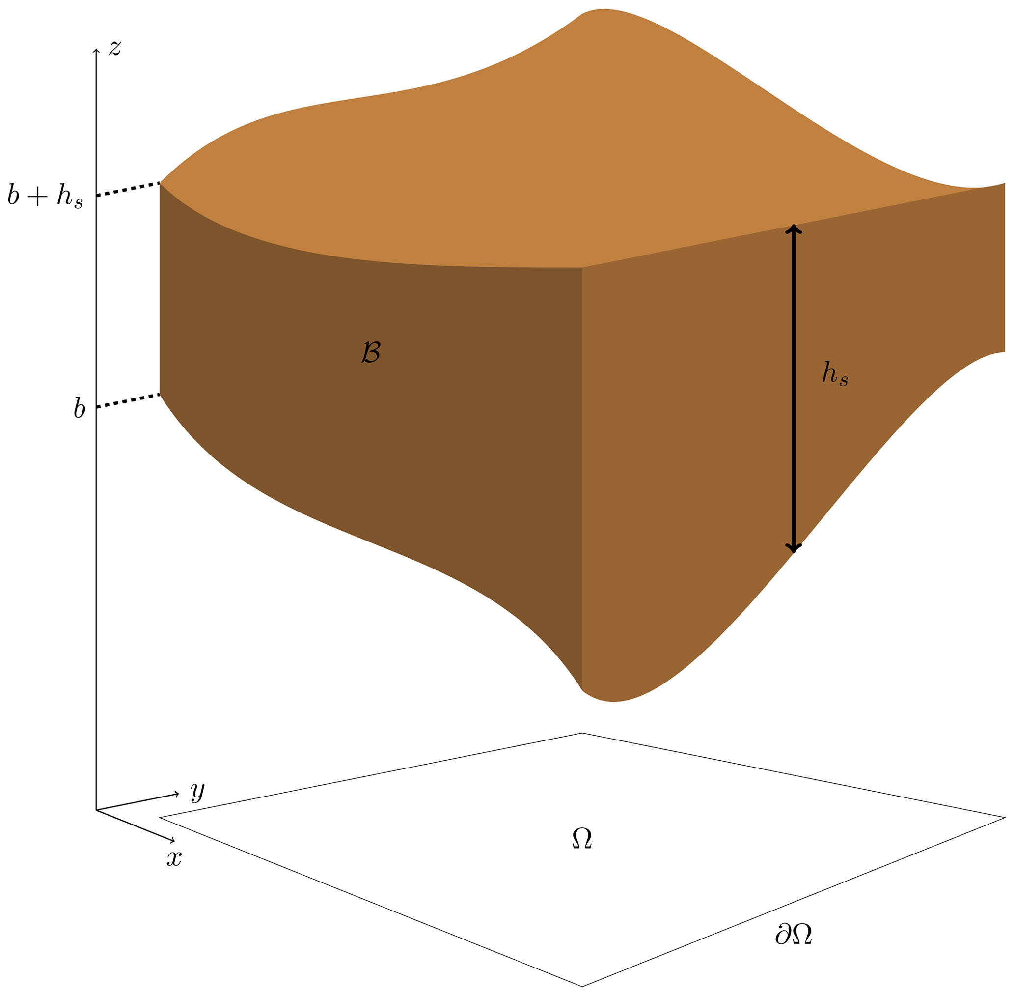
Figure 1 Representation of the two main surfaces considered in a landscape evolution model in the $(x,y,z)$ parameter space, where z is the elevation and Ω the spatial domain for (x,y) with boundary ∂Ω. The basement b surface represents the bottom part of the simulated block, on which sediments are deposited. The topographic surface is b+h_s, where h_s is the sediment thickness. The simulated sedimentary content is denoted as ℬ.

2.1 The water flow model

Landscape evolution models usually requires defining a “local discharge of water” 𝒬_w to account for water-driven erosion and transport. The practical computation of 𝒬_w, when not carefully conducted, is the weak point of many models, causing them to lose any hope of consistency in the mathematical sense of the term. It is one of the main reasons why we observe mesh dependency is some LEMs. We recall in this section how to define a physically based local discharge of water that maintains consistency. More details can be found in Coatléven (2020), Gallant and Hutchinson (2011), and Bonetti et al. (2018).

Classically, 𝒬_w is computed directly from the so-called drainage or catchment area, CA (also referred to as the contributing area). For a given outlet of the topography (i.e., the top of ℬ), it corresponds to the measure of the projection on Ω of the part of the topography from which the water contributing to this outlet is coming (Maxwell, 1870; Leopold et al., 1964; Bonetti et al., 2018). Despite being a very intuitive notion, it has evaded a precise mathematical definition for a long time. Classical multiple flow direction (MFD) algorithms are intended to provide a practical way to compute a discrete approximation CA_ϵ(K) of the catchment area, CA, for a mesh cell K (where ϵ stands for the mesh precision) and in this way a discrete approximation 𝒬_K of 𝒬_w for cell K. As is well-documented (Desmet and Govers, 1996; Pelletier, 2010, 2013; Porporato, 2022) the discrete catchment area CA_ϵ(K) obtained from those algorithms strongly depends on the cell size, geometry, and orientation with respect to the flow. Several attempts can be found in the literature to reduce this mesh dependency, defining the discrete water flow discharge 𝒬_K associated with a mesh cell K as ${\mathcal{Q}}_K=\left({\mathrm{CA}}_{\mathit{ϵ}}\right(K)/w(K\left)\right)$, where w(K) is a normalization factor related to a geometric property of the cell (see Desmet and Govers, 1996) or to an estimate of the flow width (Pelletier, 2010) defining the so-called (discrete approximation of the) specific or unit catchment area (SCA or UCA). A more modern mathematical definition of the specific catchment area a at the continuous level was proposed in Gallant and Hutchinson (2011) and Bonetti et al. (2018), consisting in solving an abstract uniform flow equation:

$$\begin{array}{}\text{(3)}& \left|\begin{array}{ll}-\mathrm{div}\left(a\frac{\mathrm{\nabla }\left(h_{\mathrm{s}}+b\right)}{\left|\right|\mathrm{\nabla }\left(h_{\mathrm{s}}+b\right)\left|\right|}\right)=\mathrm{1}& \mathrm{in}\mathrm{\Omega },\\ -a{\displaystyle \frac{\mathrm{\nabla }\left(h_{\mathrm{s}}+b\right)}{\left|\right|\mathrm{\nabla }\left(h_{\mathrm{s}}+b\right)\left|\right|}}\cdot \mathit{n}=\mathrm{0}& \mathrm{on}\partial {\mathrm{\Omega }}_{\mathrm{in}},\end{array}\right.\end{array}$$

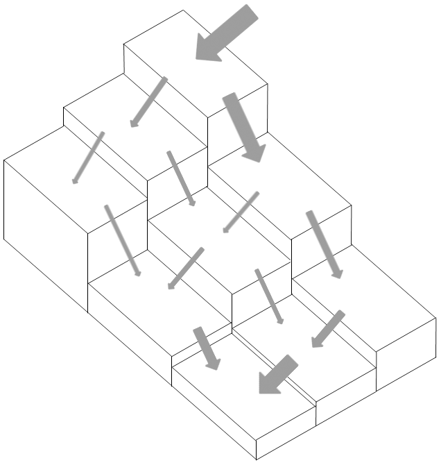
where $\partial {\mathrm{\Omega }}_{\mathrm{in}}=\mathit{\{}\mathit{x}\in \partial \mathrm{\Omega }|\mathrm{\nabla }(h_{\mathrm{s}}+b)\cdot \mathit{n}>\mathrm{0}\mathit{\}}$ is the part of the boundary that is in going and n denotes the outward normal to Ω. Setting 𝒬_w=a at the continuous level, this leads in practice to computing a consistent discrete approximation a_K of a for a mesh cell K. This allows reducing the mesh dependency to the usual consistency errors of numerical schemes. At first sight, the model in Eq. (3) could seem very different from MFD algorithms. However, considering, for instance, the classical cell-to-cell algorithms of Freeman (1989, 1991) and Holmgren (1994), one can see that those algorithms act as if we were distributing a fictitious water flow of a mesh cell to the neighboring cells with lower elevation proportionally to a function of the slope, as illustrated in Fig. 2.

Figure 2 Basic principle of the simplest cell-to-cell MFD algorithm: water is distributed to lower neighboring cells proportionally to the slope (reproduced from Coatléven, 2020).

One could then legitimately suspect that those MFD algorithms could be related to a discretization of a water flow model. This has been recently demonstrated in Coatléven (2020) for the most classical cell-to-cell MFD algorithms (for instance, those of Freeman, 1989, 1991; Holmgren, 1994). It became clear that those MFD algorithms are a way of implementing a solver for the following stationary water mass conservation with Gauckler–Manning–Strickler (GMS) flux modeling of surface runoff:

$$\begin{array}{}\text{(4)}& \left|\begin{array}{l}{\mathbf{Q}}_{\mathrm{w}}=-\frac{k_m{h}_{\mathrm{w}}{\mathit{\eta }}_{\mathrm{w}}\left(h_{\mathrm{w}}\right)}{s_{\mathrm{ref}}^{p_{\mathrm{w}}}}\left|\right|\mathrm{\nabla }(h_{\mathrm{s}}+b)\left|{|}^{p_{\mathrm{w}}}\mathrm{\nabla }\right(h_{\mathrm{s}}+b),\\ \mathrm{div}\left({\mathbf{Q}}_{\mathrm{w}}\right)=S_{\mathrm{w}}\text{ in}\mathrm{\Omega },\\ {\mathbf{Q}}_{\mathrm{w}}\cdot n=B_{\mathrm{w}}\text{ on }\partial {\mathrm{\Omega }}_{\mathrm{in}},\end{array}\right.\end{array}$$

where h_w is the water height, s_ref=1 m km⁻¹ the reference slope, p_w a model parameter, and η_w the water mobility function. For simplicity we assume here that the mobility function has no dimension and is a function of h_w only and that the domain source S_w is given in cubic meters per second per kilometer (m³ s⁻¹ km⁻²) such that its integral over a 2D area measured in square kilometers (km²) coincides with a discharge in cubic meters per second (m³ s⁻¹). The boundary influx B_w is measured in cubic meters per second per kilometer (m³ s⁻¹ km⁻¹). The coefficient k_m can be thought of as the Strickler coefficient or the inverse of the Gauckler–Manning coefficient up to a change in unit (strictly speaking, this identification is truly valid for channels and if the mobility function η_w is equal to a dimensionless hydraulic radius). For this choice of unit for S_w, k_m has the unit of a speed, i.e., meters per second (m s⁻¹). Comparing Eq. (4) with Eq. (3), we see that Eq. (3) corresponds to the particular case where k_m=1, $p_{\mathrm{w}}=-\mathrm{1}$, and a=h_wη_w(h_w). In this sense the GMS model in Eq. (4) is a generalization of Eq. (3) that allows including the classical ingredients (nonlinear slope dependency and some spatial heterogeneity) of the family of MFD algorithms.

The analysis of Coatléven (2020) explains how the discrete catchment area CA(𝒪) for the outlet of a region 𝒪 that is computed by MFD algorithms coincides with an intermediate discrete quantity appearing in the most natural discrete solver for Eq. (4). It also allows giving a continuous interpretation and generalization CA(𝒪) for any region 𝒪 of the discrete CA_ϵ that is computed by MFD algorithms only for mesh cells:

$$\begin{array}{}\text{(5)}& \begin{array}{rl}\mathrm{CA}\left(\mathcal{O}\right)=& \underset{\partial \mathcal{O}}{\int }{h}_{\mathrm{w}}{\mathit{\eta }}_{\mathrm{w}}\left(h_{\mathrm{w}}\right)\left(-k_m{s}_{\mathrm{ref}}^{-p_{\mathrm{w}}}\left|\right|\mathrm{\nabla }\left(h_{\mathrm{s}}+b\right)\right.|{|}^{p_{\mathrm{w}}}\\ & {\left.\mathrm{\nabla }\left(h_{\mathrm{s}}+b\right)\cdot \mathit{n}\right)}^{+},\end{array}\end{array}$$

where h_w is the solution of Eq. (4) with S_w=1 and where we have denoted v⁺ the positive part of v (i.e., $v^{+}=\max (\mathrm{0},v)$). Since the model in Eq. (4) describes a water flow, thanks to Coatléven (2020) we can reinterpret the discrete catchment area CA_ϵ(K) computed through the classical cell-to-cell MFD algorithms as the total flux leaving cell K of a fictitious water flow with a uniform water source S_w=1. Unfortunately, we also see that even at the continuous level, CA(𝒪) strongly depends on the geometry of 𝒪 and its orientation with respect to the flow. Since it is detailed in Coatléven (2020) that cell-to-cell MFD computations compute in practice the discrete catchment area CA_ϵ(K) for each cell K of a mesh through a discretized version of Eq. (5), as a result when MFD algorithms are used to estimate the discrete local discharge of water 𝒬_K, it produces cell and thus mesh dependency in the simulated surface water distribution. In line with the attempts of Desmet and Govers (1996) and Pelletier (2010) to define a specific catchment area (SCA) by rescaling the CA, the correct scaling would be to set the normalization factor w to the length of the portion of ∂𝒪 along which the fictitious water flow is leaving 𝒪. A corrected definition of the specific catchment at the continuous level in the spirit of Desmet and Govers (1996) and Pelletier (2010, 2013) area would thus be to use

$$\begin{array}{}\text{(6)}& \begin{array}{rl}\mathrm{SCA}\left(\mathcal{O}\right)=& {\displaystyle \frac{\mathrm{1}}{\underset{\partial \mathcal{O}}{\int }{\mathit{\chi }}_{-k_m{s}_{\mathrm{ref}}^{-p_{\mathrm{w}}}\left|\right|\mathrm{\nabla }\left(h_{\mathrm{s}}+b\right)|{|}^{p_{\mathrm{w}}}\mathrm{\nabla }\left(h_{\mathrm{s}}+b\right)\cdot \mathit{n}>\mathrm{0}}}}\underset{\partial \mathcal{O}}{\int }{h}_{\mathrm{w}}{\mathit{\eta }}_{\mathrm{w}}\left(h_{\mathrm{w}}\right)\\ & {\left(-k_m{s}_{\mathrm{ref}}^{-p_{\mathrm{w}}}\left|\right|\mathrm{\nabla }\left(h_{\mathrm{s}}+b\right)|{|}^{p_{\mathrm{w}}}\mathrm{\nabla }\left(h_{\mathrm{s}}+b\right)\cdot \mathit{n}\right)}^{+},\end{array}\end{array}$$

where χ is the indicator function (i.e., the function with value 1 when the condition is satisfied and 0 otherwise). Depending on the orientation of the flow, such a normalization will sometimes match the choices of Desmet and Govers (1996) and Pelletier (2010, 2013), explaining their partial success. This continuous SCA scales as an approximation of the continuous water flux magnitude,

$$\begin{array}{}\text{(7)}& q_{\mathrm{w}}=\left|k_m{h}_{\mathrm{w}}{\mathit{\eta }}_{\mathrm{w}}\left(h_{\mathrm{w}}\right)\right|s_{\mathrm{ref}}^{-p_{\mathrm{w}}}\left|\right|\mathrm{\nabla }\left(h_{\mathrm{s}}+b\right)|{|}^{p_{\mathrm{w}}+\mathrm{1}},\end{array}$$

(in m³ s⁻¹ km⁻¹) but is not equal to it. The SCA defined by Eq. (6) is in fact a mean of q_w along the outflow portion of ∂𝒪 and thus still retains some dependency in the geometry of 𝒪 and its orientation with respect to the flow. Meanwhile, notice that the specific catchment area a of the model in Eq. (3) can be reinterpreted through Eq. (4) as computing q_w since

$$\begin{array}{ll}{\displaystyle }{q}_{\mathrm{w}}& {\displaystyle }=\left|k_m{h}_{\mathrm{w}}{\mathit{\eta }}_{\mathrm{w}}\left(h_{\mathrm{w}}\right)\right|s_{\mathrm{ref}}^{-p_{\mathrm{w}}}\left|\right|\mathrm{\nabla }\left(h_{\mathrm{s}}+b\right)|{|}^{p_{\mathrm{w}}+\mathrm{1}}\\ {\displaystyle }& {\displaystyle }=\left|a\right|\left|\right|\mathrm{\nabla }\left(h_{\mathrm{s}}+b\right)|{|}^{-\mathrm{1}+\mathrm{1}}=a,\end{array}$$

as we have set $a=h_{\mathrm{w}}{\mathit{\eta }}_{\mathrm{w}}\left(h_{\mathrm{w}}\right)\ge \mathrm{0}$, $p_{\mathrm{w}}=-\mathrm{1}$, k_m=1, and s_ref=1 to merge Eq. (3) inside Eq. (4). Thus, in view of the success of Bonetti et al. (2018) and within the context of Eq. (4) it seems very natural to choose to set 𝒬_w=q_w. One could consider that the equivalence between classical cell-to-cell MFD algorithms established and the consistency correction proposed in Coatléven (2020) that leads to using a discrete version of q_w is another path to recover the conclusions of Eq. (3) and in this sense that q_w is a generalization of a to more complex water flow models.

The consistency correction proposed in Coatléven (2020) for MFD algorithms precisely coincides with the replacement of the computation of CA_ϵ(K) or SCA_ϵ(K) for a mesh cell K by a consistent discrete reconstruction q_K of q_w in each cell K. Convergence of this discrete version q_K to q_w when the mesh size goes to zero was proven in Coatléven (2020), along with error estimates. Thus, apart from the usual discretization error no anomalous mesh dependency should remain in q_K in practice, contrary to what is observed for SCA_ϵ(K) given by MFD algorithms. In this sense, q_K can be seen as a consistency correction for SCA_ϵ(K), as well as a generalization of Eq. (3) to a richer family of flow models. The interpretation of the local water discharge 𝒬_w as being equal to the water flux magnitude q_w given by Eq. (7) from the solution of Eq. (4) is therefore the default configuration chosen in the water flow model used to perform all the simulations we introduce in this paper.

To say that this model corresponds to the GMS model does not necessarily mean that its scope of application is limited to channels: it depends on the specific choice made on the model parameter values. Steady-state analysis (Graf and Altinakar, 2000; Birnir et al., 2001) for channels suggests using values ${\mathit{\eta }}_{\mathrm{w}}\left(h_{\mathrm{w}}\right)=(h_{\mathrm{w}}/h_{\mathrm{ref}}{)}^{\mathrm{1}/\mathrm{2}}$ and $p_{\mathrm{w}}=-\mathrm{1}/\mathrm{2}$, while the classical Gauckler–Manning–Strickler formula would coincide with ${\mathit{\eta }}_{\mathrm{w}}\left(h_{\mathrm{w}}\right)=\left(R_{\mathrm{h}}\right(h_{\mathrm{w}})/h_{\mathrm{ref}}{)}^{\mathrm{2}/\mathrm{3}}$, with R_h(h_w) the hydraulic radius and again $p_{\mathrm{w}}=-\mathrm{1}/\mathrm{2}$. When applied to large time- and space scales landscape evolution models, these calibrations are no longer valid and at this stage we suggest considering η_w and p_w as modeling parameters that can be tuned for each considered problem. In the following numerical experiments, since we only consider the water flux q_w the choice of the water mobility function has no influence and we set η_w(h_w)=1 for simplicity, as well as p_w=0. Notice that the recommendations deduced from the work discussed in this paper would remain valid for more general choices of those parameters.

The application domain of the GMS model is, however, limited by some additional requirements for the topography h_s+b. From a purely mathematical point of view, systems in Eq. (3) and Eq. (4) are in fact stationary transport problems for a or h_w. Well-posedness, i.e., existence and uniqueness in a suitable function space and continuity with respect to data, can be rigorously established only under some condition on the topography. Many different conditions are possible, all introducing some positivity requirement in the zero-order part of the differential operators applied to a or h_w (see Coatléven, 2020; Bardos, 1970; Veiga, 1987; DiPerna and Lions, 1989; Fernández-Cara et al., 2002; Girault and Tartar, 2010). In particular, among the possible conditions the simplest ones are undoubtedly

$$\begin{array}{}\text{(8)}& \begin{array}{rl}-\mathrm{\Delta }\left(h_{\mathrm{s}}+b\right)>& \mathrm{0}\mathrm{or}-\mathrm{div}\left(k_m{s}_{\mathrm{ref}}^{-p_{\mathrm{w}}}\left|\right|\mathrm{\nabla }\left(h_{\mathrm{s}}+b\right)\right.|{|}^{p_{\mathrm{w}}}\\ & \left.\mathrm{\nabla }\left(h_{\mathrm{s}}+b\right)\right)>\mathrm{0}.\end{array}\end{array}$$

By enforcing a downflow direction to exist everywhere, they both ensure that the model in Eq. (4) is well-posed, at the price of introducing quite stringent restrictions on the admissible topographies. Notice that they are sufficient conditions and not necessary ones: this implies that solutions to Eqs. (3) and (4) can still exist for some topographies not fulfilling one of the sufficient conditions. In particular, saddle-point or valley-like topographies will not easily fulfill those conditions, while it seems reasonable to assume that a solution will exist in such configurations since water can find a downflow direction. This being said, this mathematical requirement that is probably too strong should act as a warning, as it clearly reveals that not all topographies may be admissible for the model in Eq. (3) and its generalization in Eq. (4). More details on the most stringent requirements (no accumulation or flat areas) are given in Sect. 5.2.

2.2 The sediment flux model

In the present paper we have chosen to focus on the stratigraphic model that has already been discussed in detail in Granjeon (1996), Eymard et al. (2004, 2005), and Peton et al. (2020) and which is a generalization of the models studied in Smith and Bretherton (1972) and Smith et al. (1997). The corresponding sediment flux J_s takes the following form:

$$\begin{array}{}\text{(9)}& \begin{array}{rl}{\mathit{J}}_{\mathrm{s}}=& -{\mathit{\eta }}_{\mathrm{s}}\left(h_{\mathrm{s}}\right)s_{\mathrm{ref}}^{-p_{\mathrm{s}}}\left|\right|\mathrm{\nabla }\left(h_{\mathrm{s}}+b\right)|{|}^{p_{\mathrm{s}}}\left({\left({\displaystyle \frac{q_{\mathrm{w}}}{q_{\mathrm{ref}}}}\right)}^{r_{\mathrm{s}}}\right.\\ & \left.\mathrm{\nabla }{\mathit{\psi }}_{\mathrm{w}}\left(h_{\mathrm{s}}+b\right)+\mathrm{\nabla }{\mathit{\psi }}_{\mathrm{g}}\left(h_{\mathrm{s}}+b\right)\right)\mathrm{in}\mathrm{\Omega }\times ]t_{\mathrm{0}},T[,\end{array}\end{array}$$

where r_s>0 and p_s>0 are model parameters, q_w is the water flux obtained from Eq. (4), q_ref and s_ref are dimensional factors, and η_s is a dimensionless sediment mobility function such that

$$\begin{array}{}\text{(10)}& \begin{array}{ll}\mathrm{0}\le {\mathit{\eta }}_{\mathrm{s}}\left(h_{\mathrm{s}}\right)\le \mathrm{1}& \mathrm{and}{\mathit{\eta }}_{\mathrm{s}}\left(\mathrm{0}\right)=\mathrm{0},\end{array}\end{array}$$

whose main role is to ensure that the sediment height h_s remains positive. In the following we use

$$\begin{array}{}\text{(11)}& {\mathit{\eta }}_{\mathrm{s}}\left(h_{\mathrm{s}}\right)=\left|\begin{array}{ll}\mathrm{1}-\frac{h_{\mathrm{c}}}{h_{\mathrm{s}}+h_{\mathrm{c}}}& \mathrm{if}{h}_{\mathrm{s}}\ge \mathrm{0},\\ \mathrm{0}& \mathrm{otherwise},\end{array}\right.\end{array}$$

with h_c a parameter. The function with subscript “w” is intended to model the water-driven processes, while the function with subscript “g” models gravity-related processes. We consider here the most common form for functions ψ_w and ψ_g corresponding to

$$\begin{array}{}\text{(12)}& {\mathit{\psi }}_{\mathrm{w}}\left(h_{\mathrm{s}}+b\right)=\underset{\mathrm{0}}{\overset{h_{\mathrm{s}}+b}{\int }}{k}_{\mathrm{w}}\left(v\right)\mathrm{d}v\mathrm{and}{\mathit{\psi }}_{\mathrm{g}}\left(h_{\mathrm{s}}+b\right)=\underset{\mathrm{0}}{\overset{h_{\mathrm{s}}+b}{\int }}{k}_{\mathrm{g}}\left(v\right)\mathrm{d}v,\end{array}$$

where k_w and k_g are bounded diffusion coefficients depending solely on h_s in such a way that

$$\begin{array}{}\text{(13)}& \begin{array}{rl}& \mathrm{\nabla }{\mathit{\psi }}_{\mathrm{w}}\left(h_{\mathrm{s}}+b\right)=k_{\mathrm{w}}\left(h_{\mathrm{s}}+b\right)\mathrm{\nabla }\left(h_{\mathrm{s}}+b\right)\mathrm{and}\\ & \mathrm{\nabla }{\mathit{\psi }}_{\mathrm{g}}\left(h_{\mathrm{s}}+b\right)=k_{\mathrm{g}}\left(h_{\mathrm{s}}+b\right)\mathrm{\nabla }\left(h_{\mathrm{s}}+b\right),\end{array}\end{array}$$

so the sediment flux follows the topographic slope ∇(h_s+b).

This sediment flux model is implemented in our modeling platform ArcaDES, and all the simulations shown in the following sections are performed using the ArcaDES platform (although ArcaDES is mentioned for the first time in a scientific paper, it has been used since 2015 in the stratigraphic numerical forward model DionisosFlow^TM initially developed by Granjeon, 1996). Both soil erosion and sediment deposition are considered. As ArcaDES is designed for large-scale simulations in time and space, we have chosen to express the x–y coordinates in kilometers (km), time in millions of years (Myr), and sediment height h_s and basement b in meters (m). Thus, the unit for sediment sources will be meters per million years (m Myr⁻¹). Since we have chosen to use 𝒬_w=q_w with q_w the water flux from Eq. (4), the unit for the water discharge q_w is cubic meters per second per kilometer (m³ s⁻¹ km⁻¹), and thus we naturally set q_ref=1 m³ s⁻¹ km⁻¹. The natural unit of coefficients k_g and k_w is square kilometer per million years (km² Myr⁻¹), with the reference slope again set to s_ref=1 m km⁻¹.

2.3 Some insights from perturbation theory

In this subsection, in order to give a feeling of the potential stability issues related to the model in Eqs. (2)–(9)–(4), we will perform a brief analysis of the behavior of solutions under perturbations. Details of the following computation are relegated to Appendix A. We assume for simplicity that k_g and k_w are constant functions. Let us denote ($h_{\mathrm{s},*},h_{\mathrm{w},*}$) a reference solution of Eqs. (2)–(9)–(4) with sources ($S_{\mathrm{s},*},S_{\mathrm{w},*}$), whose stability is to be tested. We denote ($h_{\mathrm{s},\mathit{\delta }},h_{\mathrm{w},\mathit{\delta }}$) a perturbation of magnitude δ of this reference solution associated with the source perturbation ($S_{\mathrm{s},\mathit{\delta }},S_{\mathrm{w},\mathit{\delta }}$) and consider the evolution of ($h_{\mathrm{s}},h_{\mathrm{w}})=(h_{\mathrm{s},*}+h_{\mathrm{s},\mathit{\delta }},h_{\mathrm{w},*}+h_{\mathrm{w},\mathit{\delta }}$) for the perturbed source ($S_{\mathrm{s},*}+S_{\mathrm{s},\mathit{\delta }},S_{\mathrm{w},*}+S_{\mathrm{w},\mathit{\delta }}$). Since both the perturbed and unperturbed solutions have to satisfy the boundary conditions, we deduce that the perturbation ($h_{\mathrm{s},\mathit{\delta }},h_{\mathrm{w},\mathit{\delta }}$) itself also satisfies the same boundary conditions. Then, in line with, for instance, the analysis of Smith et al. (1997), injecting (h_s,h_w) into Eqs. (2)–(9), multiplying by h_s,δ, and integrating by parts we obtain the equation governing the evolution of the perturbation's total energy (see Appendix A for details):

$$\begin{array}{}\text{(14)}& \begin{array}{rl}{\displaystyle \frac{\mathrm{d}}{\mathrm{d}t}}\left({\displaystyle \frac{\mathrm{1}}{\mathrm{2}}}\underset{\mathrm{\Omega }}{\int }{h}_{\mathrm{s},\mathit{\delta }}^{\mathrm{2}}\right)& =-\underset{\mathrm{\Omega }}{\int }{j}_{\mathrm{s}}\left(h_{\mathrm{s}},h_{\mathrm{s}}+b,q_{\mathrm{w}}\right)\left|\right|\mathrm{\nabla }{h}_{\mathrm{s},\mathit{\delta }}|{|}^{\mathrm{2}}\\ & +\underset{\mathrm{\Omega }}{\int }{S}_{\mathrm{s},\mathit{\delta }}{h}_{\mathrm{s},\mathit{\delta }}+\underset{\mathrm{\Omega }}{\int }\left(j_{\mathrm{s}}\left(h_{\mathrm{s},*},h_{\mathrm{s},*}+b,q_{\mathrm{w},*}\right)\right.\\ & \left.-j_{\mathrm{s}}\left(h_{\mathrm{s}},h_{\mathrm{s}}+b,q_{\mathrm{w}}\right)\right)\mathrm{\nabla }\left(h_{\mathrm{s},*}+b\right)\cdot \mathrm{\nabla }{h}_{\mathrm{s},\mathit{\delta }},\end{array}\end{array}$$

where we have denoted

$$j_{\mathrm{s}}(u,v,w)={\mathit{\eta }}_{\mathrm{s}}\left(u\right)s_{\mathrm{ref}}^{-p_{\mathrm{s}}}\left|\right|\mathrm{\nabla }v|{|}^{p_{\mathrm{s}}}\left({\left({\displaystyle \frac{w}{q_{\mathrm{ref}}}}\right)}^{r_{\mathrm{s}}}{k}_{\mathrm{w}}+k_{\mathrm{g}}\right).$$

The first term of the right-hand side is always negative and thus always contributes to the stability of the system. The second term describes the contribution of potential perturbation sources S_s,δ (other than the initial conditions) to the evolution of the perturbation's energy. The last term,

$$\begin{array}{}\text{(15)}& \begin{array}{rl}{A}_{\mathit{\delta }}=& \underset{\mathrm{\Omega }}{\int }\left(j_{\mathrm{s}}\left(h_{\mathrm{s},*},h_{\mathrm{s},*}+b,q_{\mathrm{w},*}\right)-j_{\mathrm{s}}\left(h_{\mathrm{s}},h_{\mathrm{s}}+b,q_{\mathrm{w}}\right)\right)\\ & \mathrm{\nabla }\left(h_{\mathrm{s},*}+b\right)\cdot \mathrm{\nabla }{h}_{\mathrm{s},\mathit{\delta }},\end{array}\end{array}$$

originates partially from the nonlinearity of the sediment transport model but most importantly from the coupling between the flow and the sediment transport. If A_δ is negative or sufficiently small and if the perturbation source is also small enough, then the sediment perturbation energy will decrease with time. In this case, the solution ($h_{\mathrm{s},*},h_{\mathrm{w},*}$) is said to be stable under perturbation ($h_{\mathrm{s},\mathit{\delta }},h_{\mathrm{w},\mathit{\delta }}$). However, the sign of A_δ is not always negative and will often take non-necessarily small positive values. If A_δ is large enough, instead of being diffused by the first term the sediment perturbation energy will grow with time and potentially become as large as the unperturbed solution: the solution ($h_{\mathrm{s},*},h_{\mathrm{w},*}$) is then unstable under perturbation ($h_{\mathrm{s},\mathit{\delta }},h_{\mathrm{w},\mathit{\delta }}$). This is a self-amplification mechanism, as the magnitude of A_δ will grow with the perturbation's magnitude and cancel if the perturbation is zero, and also because of the dependency of the water flux q_w,δ on the topography perturbation h_s,δ. We will say that growing perturbations correspond to the physically unstable regime.

We can anticipate that the relative magnitude of the gravity and water coefficients k_g and k_w will play a key role in the stability of solutions. Indeed denoting $\mathit{\tau }=\left(k_{\mathrm{w}}{q}_{\mathrm{w}}^{r_{\mathrm{s}}}\right)/\left(k_{\mathrm{g}}{q}_{\mathrm{ref}}^{r_{\mathrm{s}}}\right)$, if k_g is much larger than k_w and thus τ is very small we have, assuming for simplicity that η_s=1 (see Appendix A for details),

$$\begin{array}{ll}{\displaystyle }{A}_{\mathit{\delta }}& {\displaystyle }\approx -k_{\mathrm{g}}{s}_{\mathrm{ref}}^{-p_{\mathrm{s}}}\left(p_{\mathrm{s}}\left|\right|\mathrm{\nabla }\left(h_{\mathrm{s},*}+b\right)\left|{|}^{p_{\mathrm{s}}-\mathrm{2}}\right|\mathrm{\nabla }\left(h_{\mathrm{s},*}+b\right)\cdot \mathrm{\nabla }{h}_{\mathrm{s},\mathit{\delta }}{|}^{\mathrm{2}}\right)\\ {\displaystyle }& {\displaystyle }+O\left(\mathit{\tau }\right)+O\left({\mathit{\delta }}^{\mathrm{3}}\right)\end{array}$$

(where we recall that a function f is O(h), there exists a constant C>0 independent of h such that $\left|\right|f\left|\right|\le Ch$ for a suitable norm $\left|\right|.\left|\right|$). Then for large values of k_g the term A_δ is always negative and thus stabilizing. On the contrary, if k_w is much larger than k_g then τ is also very large and we have (see Appendix A for details)

$$\begin{array}{ll}{\displaystyle }{A}_{\mathit{\delta }}& {\displaystyle }\approx -k_{\mathrm{w}}{s}_{\mathrm{ref}}^{-p_{\mathrm{s}}}{r}_{\mathrm{s}}{\displaystyle \frac{q_{\mathrm{w},*}^{r_{\mathrm{s}}-\mathrm{1}}}{q_{\mathrm{ref}}^{r_{\mathrm{s}}}}}{q}_{\mathrm{w},\mathit{\delta }}\left|\right|\mathrm{\nabla }\left(h_{\mathrm{s},*}+b\right)|{|}^{p_{\mathrm{s}}}\mathrm{\nabla }\left(h_{\mathrm{s},*}+b\right)\\ {\displaystyle }& {\displaystyle }\cdot \mathrm{\nabla }{h}_{\mathrm{s},\mathit{\delta }}-k_{\mathrm{w}}{s}_{\mathrm{ref}}^{-p_{\mathrm{s}}}{\left({\displaystyle \frac{q_{\mathrm{w},*}}{q_{\mathrm{ref}}}}\right)}^{r_{\mathrm{s}}}\left(p_{\mathrm{s}}\left|\right|\mathrm{\nabla }\left(h_{\mathrm{s},*}+b\right)\left|{|}^{p_{\mathrm{s}}-\mathrm{2}}\right|\mathrm{\nabla }\right.\\ {\displaystyle }& {\displaystyle }\left.\left(h_{\mathrm{s},*}+b\right)\cdot \mathrm{\nabla }{h}_{\mathrm{s},\mathit{\delta }}{|}^{\mathrm{2}}\right)+O(\mathrm{1}/\mathit{\tau })+O\left({\mathit{\delta }}^{\mathrm{3}}\right).\end{array}$$

Regions for which $\mathrm{\nabla }(h_{\mathrm{s},*}+b)\cdot \mathrm{\nabla }{h}_{\mathrm{s},\mathit{\delta }}<\mathrm{0}$ will amplify the perturbation proportionally to k_w and the power r_s−1 of the water flux. We also see that the term A_δ will behave quite differently if r_s>1 or r_s<1. Indeed, for r_s>1 the water flux will reinforce the amplification term in a kind of positive feedback loop. On the contrary, for r_s<1 the water flux will temper the amplification term, and thus we can anticipate that it will require much larger values of τ for instability to occur in this situation. For the general case incorporating η_s the behavior is roughly speaking the same, with the main difference that the additional term due to η_s can on rare occasions also contribute with the wrong sign (see Appendix A for details). The main conclusion to draw from this brief study is that parameter τ will be the main criterion governing the appearance of instabilities even for our most general model.

For a subclass of model equations, Eqs. (2)–(9)–(4), with η_s=1, k_g=0 and $p_{\mathrm{w}}=-\mathrm{1}$ and p_s=0, the stability of solutions have been theoretically studied in Smith and Bretherton (1972) and Smith et al. (1997). This would correspond within our notations to the extreme case where $\mathit{\tau }=+\mathrm{\infty }$, for which we expect instability to occur. It was, for instance, established in Smith et al. (1997) that if the reference solution is stationary, the second term is negative only if some specific condition on the gradient ∇(h_s+b) is satisfied on the boundary of the region of interest, here Ω. The linear stability of analytic stationary solutions that are uniform in one direction has also been considered in Smith et al. (1997). Their conclusion is that under periodic perturbations in the transverse direction, for r_s≤1, the linear stability analysis does not reveal any instability, while for r_s>1, the stationary solutions are linearly unstable if the frequency of the periodic perturbation is large enough. This is coherent with the above brief perturbation study. Notice that the case $p_{\mathrm{w}}=-\mathrm{1}$ greatly simplifies such studies: the linear stability analysis can be shown to be equivalent to solving a one-dimensional ordinary differential equation.

The studies mentioned above are focused on the stability of physically meaningful solutions. Here, we want to draw attention to the numerical consequences of this self-amplification phenomenon; in this way we focus on the stability of numerical solutions. Let us explain the key idea: assuming that all functions are regular enough, one could consider (for instance in a finite-difference setting) that our numerical solution is roughly speaking a perturbation of the exact continuous solution, where the source terms S_s,δ and S_w,δ represent the unavoidable consistency and solver errors of our solving process. Then the numerical sediment perturbation energy will satisfy Eq. (14) and will self-amplify in the same way that physical perturbations self-amplify. In the unstable regime, this means that the numerical solution can potentially diverge from the exact solution from a large amount up to the point that it cannot be considered a relevant approximation of the continuous solution, even if the numerical perturbation arises from initially small numerical errors. In other words, in the absence of any treatment, numerical errors may dominate the geomorphological responses of the systems. However, since these numerical errors are reworked by a system of physical equations, it is not impossible to obtain good-looking results. This is where the trap lies for the modeler, who might be inclined to interpret a result induced by uncontrolled numerical noise as a physically plausible solution.

3 Numerical instabilities arising from the nonlinear coupling of overland flow and sediment dynamic

To illustrate the numerical issues linked to the self-amplification of initially small numerical errors, we consider in this section several situations where we have either full knowledge of the exact solution or a criterion to distinguish it from incorrect solutions. Thanks to this information on the exact solution, we can illustrate the stability issues of simulations using the model in Eqs. (2)–(9)–(4) (discretized by the finite-volume scheme detailed in Appendix C).

3.1 Instabilities for analytic solutions

In this subsection we consider stationary analytic functions of the form

$$\left|\begin{array}{l}{h}_{\mathrm{s}}^{\mathrm{ex}}(x,y)=h_{\mathrm{s},x}\left(x\right)+\sum _{p=\mathrm{1}}^{N_{\mathrm{b}}}{g}_{\mathrm{b}}\left(\frac{x-x_{\mathrm{p}}}{{\mathit{\delta }}_x},\frac{y-y_{\mathrm{p}}}{{\mathit{\delta }}_y}\right),\\ h_{\mathrm{w}}^{\mathrm{ex}}(x,y)=h_{\mathrm{w},x}\left(x\right),\end{array}\right.$$

incorporating N_b small smooth bumps randomly positioned at points (x_p,y_p) chosen such that they do interfere with the boundary conditions, with the smooth bump function given by

$$\begin{array}{ll}{\displaystyle }& {\displaystyle }{g}_{\mathrm{b}}(x,y)=g_{\mathrm{b}}\left(r^{\mathrm{2}}\right)=\\ {\displaystyle }& {\displaystyle }\left|\begin{array}{ll}{H}_{\mathrm{pert}}\exp \left(\frac{-\mathit{\gamma }}{\mathrm{1}-r^{\mathrm{2}}}\right)\exp \left(\mathit{\gamma }\right)& \mathrm{for}{r}^{\mathrm{2}}=x^{\mathrm{2}}+y^{\mathrm{2}}\le \mathrm{1},\\ \mathrm{0}& \mathrm{otherwise},\end{array}\right.\end{array}$$

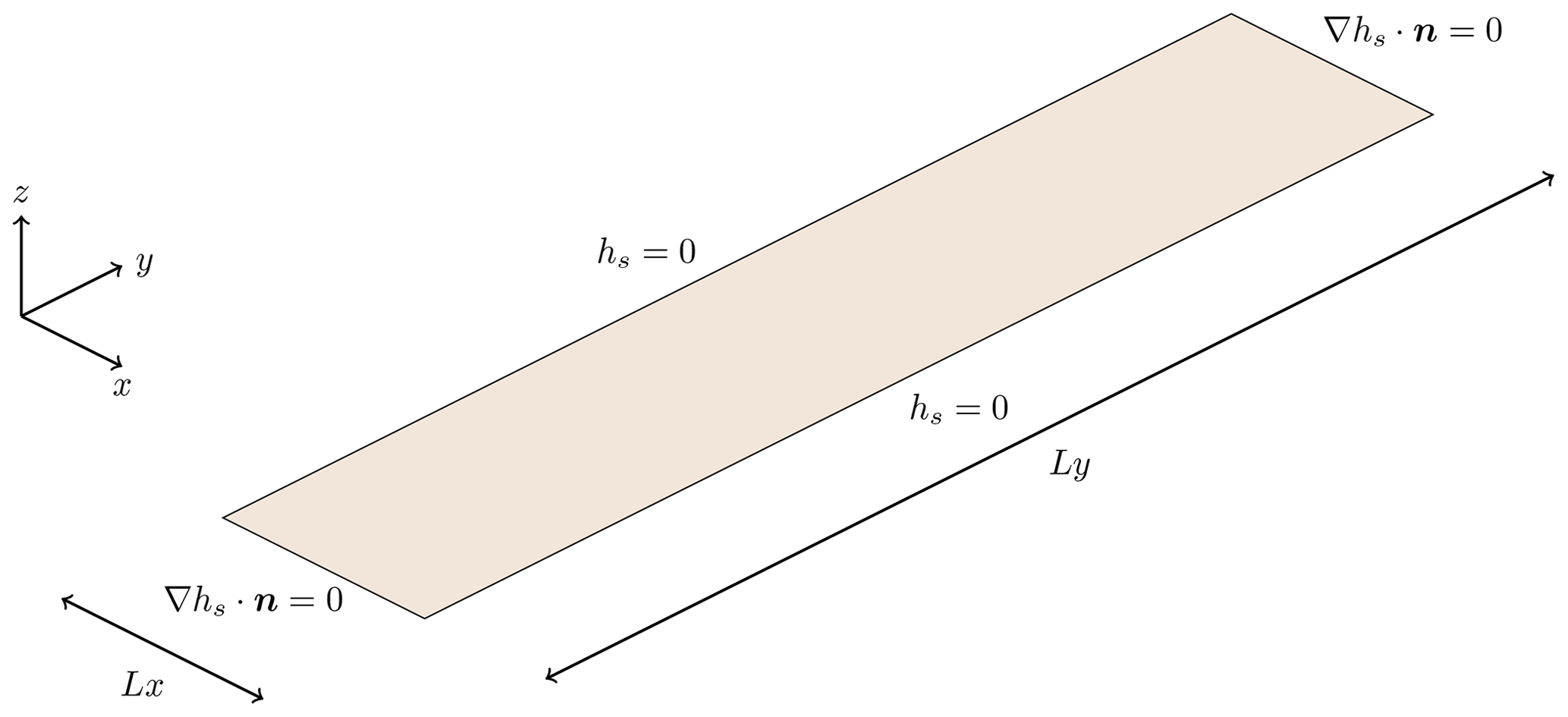
with in practice N_b=5, H_pert=0.03 m, γ=10, and ${\mathit{\delta }}_x={\mathit{\delta }}_y=\mathrm{0.25}$ km. The numerical domain is rectangular and centered at (0, 0) with the dimensions Lx=1 km on the x axis and Ly=5 km on the y axis, and the basement b is set to zero. We impose homogeneous Dirichlet boundary conditions (h_s=0) on the boundaries $y=-Lx/\mathrm{2}$ and $x=Lx/\mathrm{2}$ and homogeneous Neumann boundary conditions (${\partial }_y{h}_{\mathrm{s}}=\mathrm{0}$) on the boundaries $y=-Ly/\mathrm{2}$ and $y=Ly/\mathrm{2}$ as illustrated in Fig. 3.

Figure 3 Domain configuration for the analytic tests cases.

We use for the mono-dimensional functions ($h_{\mathrm{s},x},h_{\mathrm{w},x}$) the stationary solution of the model in Eqs. (2)–(9)–(4) in the case η_s=1 given in Appendix D that satisfies the boundary conditions. For all our simulations, the constant source terms ($S_{\mathrm{s},x},S_{\mathrm{w},x}$) for the analytic the stationary solution ($h_{\mathrm{s},x},h_{\mathrm{w},x}$) in the case η_s=1 (see Appendix D for details) are always equal to (10 m Myr⁻¹, 1 m³ s⁻¹ km⁻²). Injecting (h_s,h_w) into Eqs. (2)–(9)–(4), after some straightforward but tedious computations one can derive exact expressions for the corresponding source terms ($S_{\mathrm{s}}^{\mathrm{ex}},S_{\mathrm{w}}^{\mathrm{ex}}$), making the pair (h_s,h_w) an analytic solution of our model for those source terms.

Given those analytic source terms, initializing the sediment height to the analytic value $h_{\mathrm{s}}(x,y,\mathrm{0})=h_{\mathrm{s}}^{\mathrm{ex}}(x,y)$ and the water height to the analytic value $h_{\mathrm{w}}(x,y,\mathrm{0})=h_{\mathrm{w}}^{\mathrm{ex}}(x,y)$ the exact solution of the model in Eqs. (2)–(9)–(4) is of course simply equal to ($h_{\mathrm{s}}^{\mathrm{ex}},h_{\mathrm{w}}^{\mathrm{ex}}$) for all times. Thus, any reasonable numerical solution should remain a correct approximation of ($h_{\mathrm{s}}^{\mathrm{ex}},h_{\mathrm{w}}^{\mathrm{ex}}$) for all times. Using the finite-volume discretization described in Appendix C on a Cartesian mesh with square cells for which we denote Δ_xy the size of the edges of the Cartesian cells, we attempt to reproduce the stationary analytic solution by initializing the system to ($h_{\mathrm{s}}(x,y,\mathrm{0}),h_{\mathrm{w}}(x,y,\mathrm{0}))=(h_{\mathrm{s}}^{\mathrm{ex}}(x,y),h_{\mathrm{w}}^{\mathrm{ex}}(x,y)$) and using the analytic source terms ($S_{\mathrm{s}}^{\mathrm{ex}},S_{\mathrm{w}}^{\mathrm{ex}}$) for various values of the parameters k_g, k_w, r_s, and p_s. The simulation total time is 0.25 Myr, and we use time steps of maximum length Δt=0.002 Myr. The corresponding analytic solutions are presented in Figs. 4–8 for the different values of the parameters k_g, k_w, r_s, and p_s we have considered. All those simulations have been performed in parallel on 108 processors using the MPI library. In Fig. 9, we present the obtained convergence curves for all the tested analytic solutions; i.e., we plot the standard L² error measuring the difference between the simulated sediment height and the exact analytic sediment height. We see in Fig. 9 that for all configurations except the case (k_g=1 km² Myr⁻¹, k_w=50 km² Myr⁻¹), we obtain clean convergences curves, assessing the correctness of our numerical scheme even for the nonlinear couplings. However, for the case (k_g=1 km² Myr⁻¹, k_w=50 km² Myr⁻¹) the two nonlinear couplings ($r_{\mathrm{s}}=\mathrm{3}/\mathrm{2}$, p_s=1) and (r_s=2, p_s=0) fail to converge. Looking at Table 1 where we regroup the value of τ for each test case using our knowledge of the exact solution, we see that convergence problems appear as expected when τ becomes large. Indeed, since the error increases when we refine the mesh, this error is not a discretization consistency error as all the other test cases validate both our implementation and discretization. On the contrary, it increases with the size of the numerical system, which strongly suggests that it originates from solver (both linear and nonlinear) errors, and this perfectly illustrates the phenomenon of numerical error self-amplification that we have discussed from a theoretical point of view in the Sect. 2.3. Problems are potentially more severe in finer meshes because numerical diffusion that can dissipate residual numerical errors declines with grid spacing. Now, to illustrate how treacherous those numerical solutions are, we present in Figs. 10 and 11 a comparison between the analytic solution and its erroneous numerical counterpart. The erroneous solutions are dangerously “good-looking”: indeed, if only the initial topography and the rain and production data are shown, one could easily be tempted to interpret the quite complex topographies obtained as the realistic self-amplification of the perturbations due to the presence of the bumps. However, since we know the exact solution, we are sure that this is not the case: the appealing numerical solutions are completely wrong. The overall “geologically realistic” look of the erroneous solution comes from the fact that numerical noise is amplified not by some numerical scheme deficiency but by the capacity of the continuous model to amplify perturbations that we describe in the previous section. In other words, the numerical noise is reworked by the system, giving a “realistic” look to it. This is the reason why we stress that when performing real-life simulations for which of course the correct solution is unknown (otherwise we would not need to simulate anything at all), it can become very hard to decide if the numerical results are correct or blurred by realistic-looking amplified numerical noise. The quality of the numerical scheme, although essential, is not in question: the issue is the self-amplification mechanisms of the continuous model. They are the reason for its physical interest but simultaneously its main issue for performing reliable simulations.

Table 1 Approximate maximum analytic value of $\mathit{\tau }=\frac{k_{\mathrm{w}}}{k_{\mathrm{g}}}{\left(\frac{q_{\mathrm{w}}}{q_{\mathrm{ref}}}\right)}^{r_{\mathrm{s}}}$ for each convergence test.

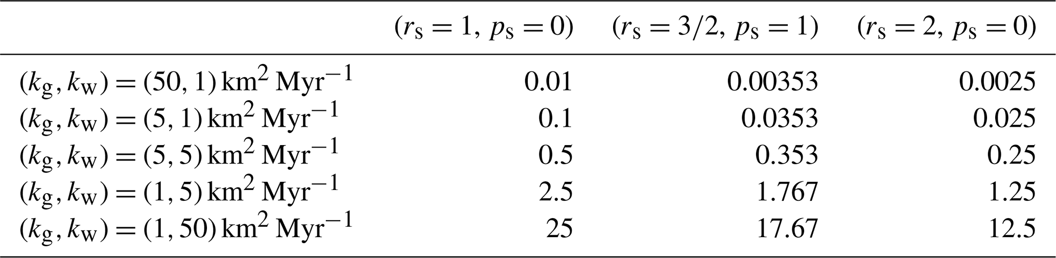
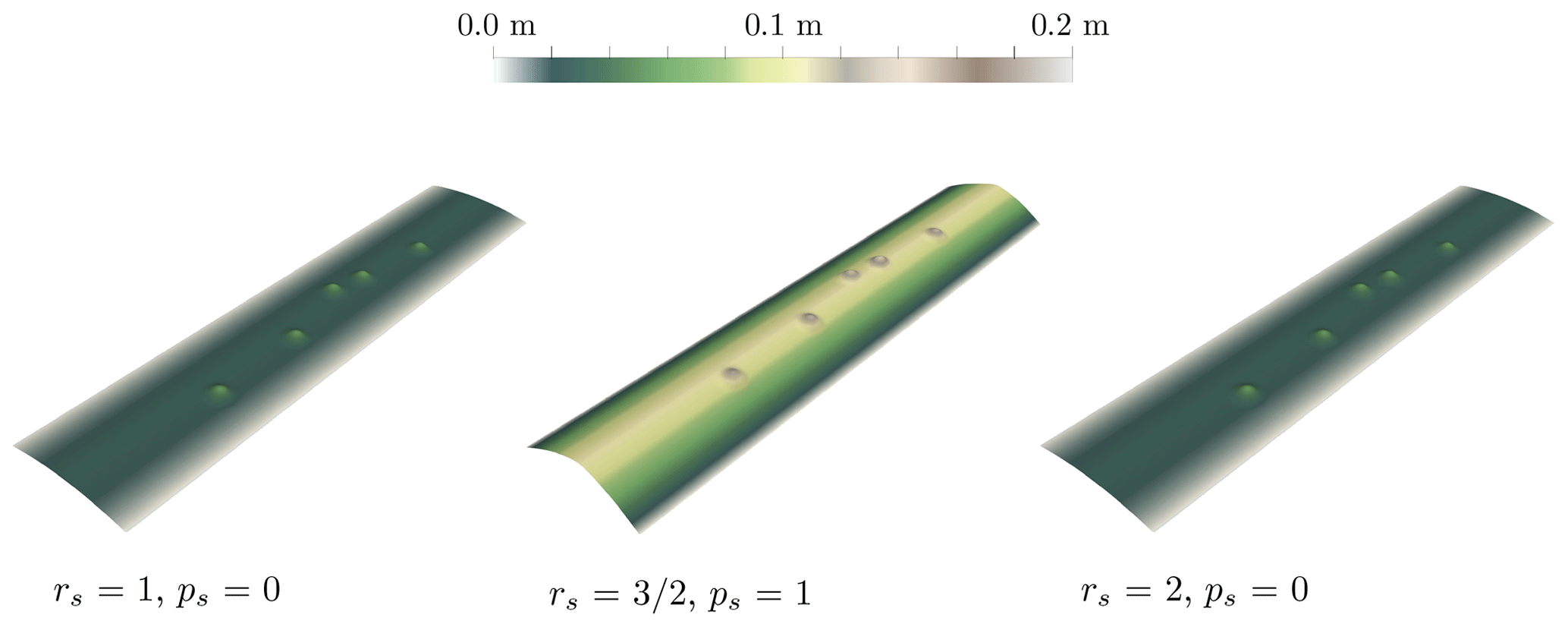
Figure 4 Sediment height $h_{\mathrm{s}}^{\mathrm{ex}}$ of the analytic solution for the case k_g=50 km² Myr⁻¹ and k_w=1 km² Myr⁻¹.

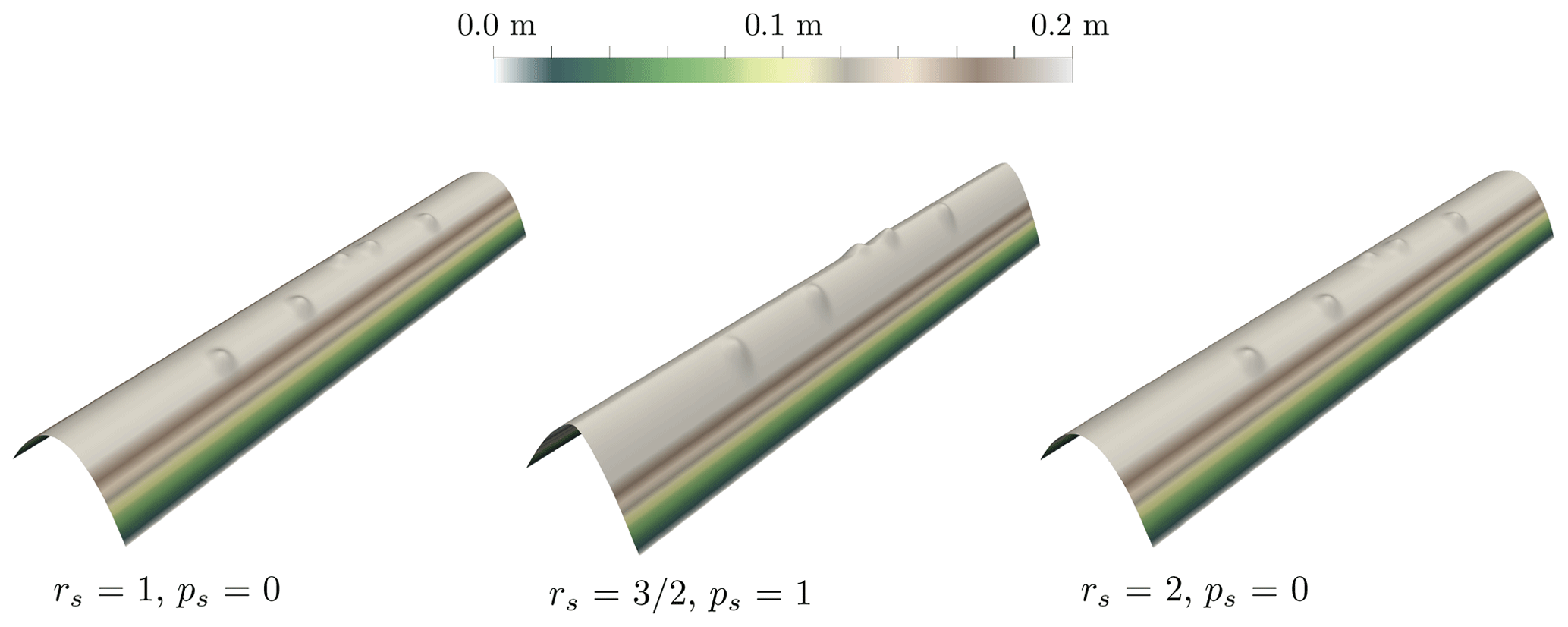
Figure 5 Sediment height $h_{\mathrm{s}}^{\mathrm{ex}}$ of the analytic solution for the case k_g=5 km² Myr⁻¹ and k_w=1 km² Myr⁻¹.

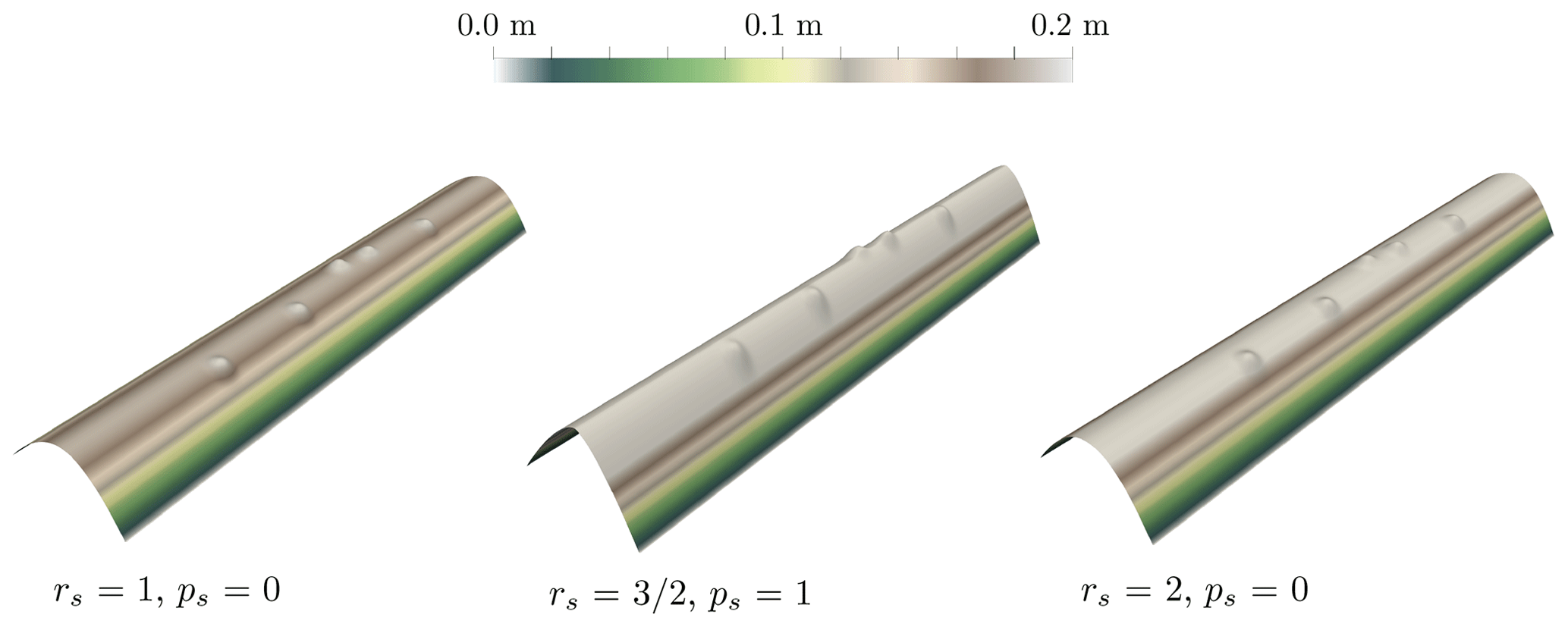
Figure 6 Sediment height $h_{\mathrm{s}}^{\mathrm{ex}}$ of the analytic solution for the case k_g=5 km² Myr⁻¹ and k_w=5 km² Myr⁻¹.

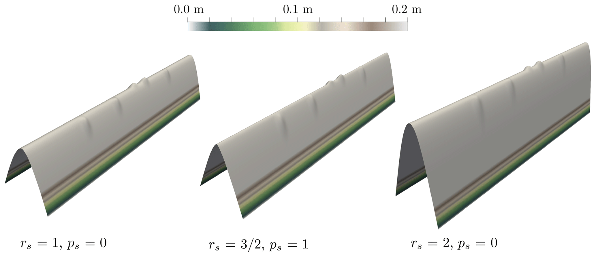
Figure 7 Sediment height $h_{\mathrm{s}}^{\mathrm{ex}}$ of the analytic solution for the case k_g=1 km² Myr⁻¹ and k_w=5 km² Myr⁻¹.

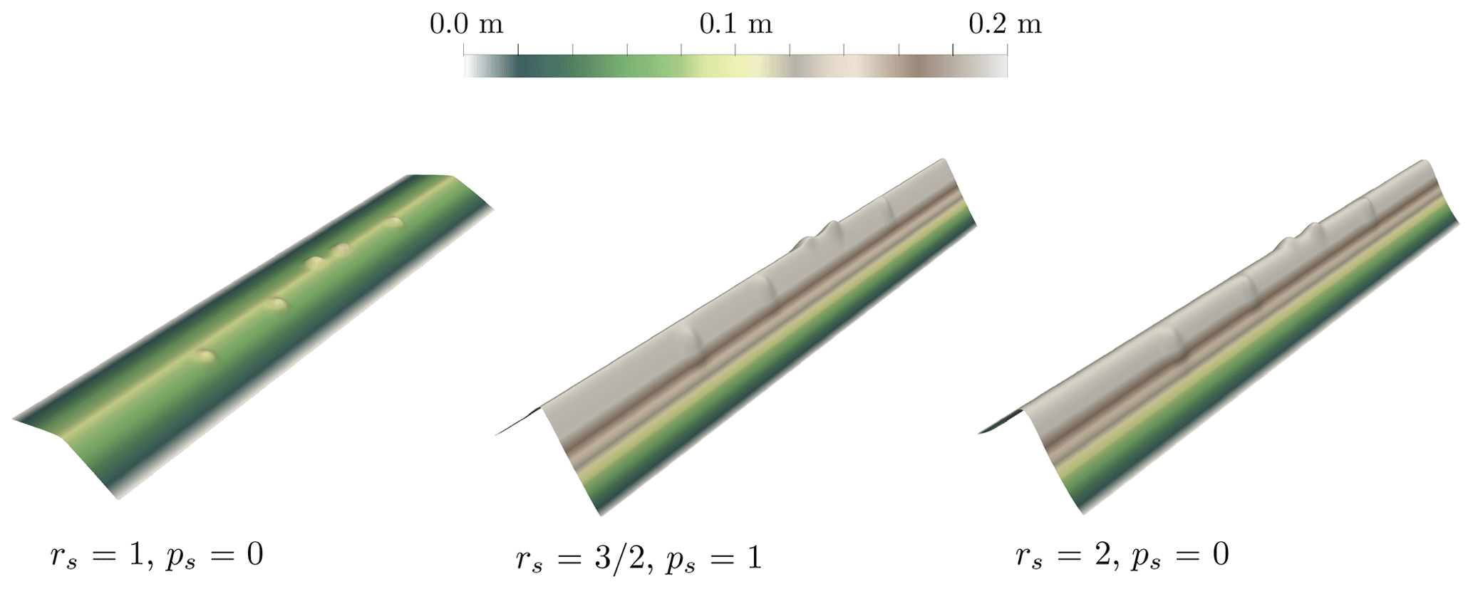
Figure 8 Sediment height $h_{\mathrm{s}}^{\mathrm{ex}}$ of the analytic solution for the case k_g=1 km² Myr⁻¹ and k_w=50 km² Myr⁻¹.

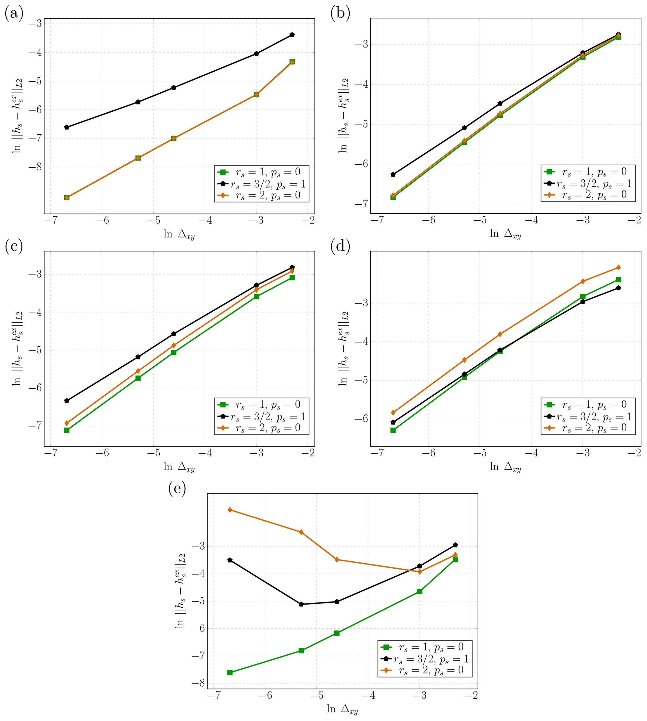
Figure 9 Convergence curves. (a) Case k_g=50 km² Myr⁻¹ and k_w=1 km² Myr⁻¹. (b) Case k_g=5 km² Myr⁻¹ and k_w=1 km² Myr⁻¹. (c) Case k_g=5 km² Myr⁻¹ and k_w=5 km² Myr⁻¹. (d) Case k_g=1 km² Myr⁻¹ and k_w=5 km² Myr⁻¹. (e) Case k_g=1 km² Myr⁻¹ and k_w=50 km² Myr⁻¹.

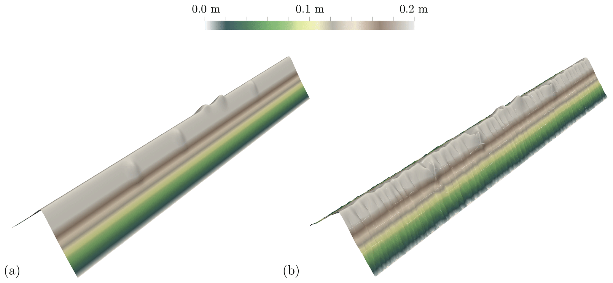
Figure 10 Comparison between the sediment height $h_{\mathrm{s}}^{\mathrm{ex}}$ of the analytic solution and numerical solution h_s for the case k_g=1 km² Myr⁻¹, k_w=50 km² Myr⁻¹, $r_{\mathrm{s}}=\mathrm{3}/\mathrm{2}$, and p_s=1. (a) Analytic solution $h_{\mathrm{s}}^{\mathrm{ex}}$ and (b) numerical solution h_s.

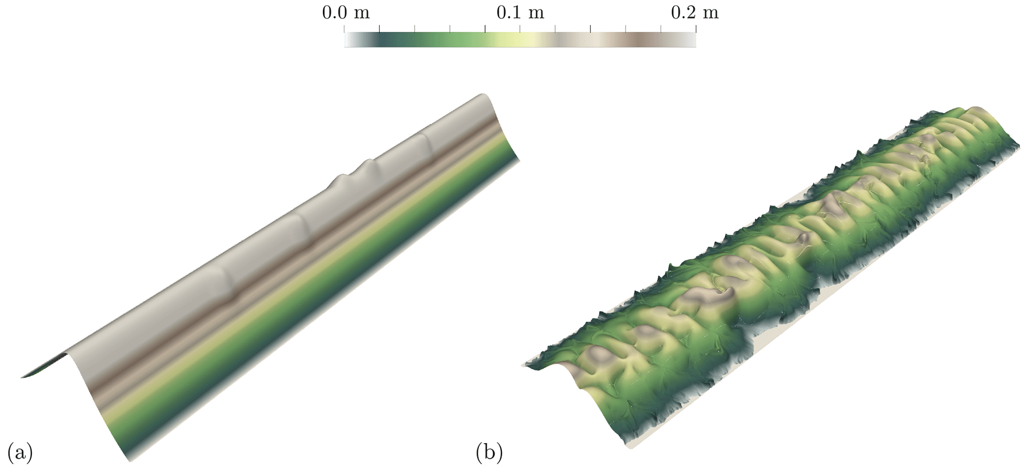
Figure 11 Comparison between the sediment height $h_{\mathrm{s}}^{\mathrm{ex}}$ of the analytic solution and numerical solution h_s for the case k_g=1 km² Myr⁻¹, k_w=50 km² Myr⁻¹, r_s=2, and p_s=0. (a) Analytic solution $h_{\mathrm{s}}^{\mathrm{ex}}$ and (b) numerical solution h_s.

3.2 Identifiable instabilities in a non-analytic case

As previously mentioned, having an analytical solution is quite rare when it comes to applying the model in Eq. (2) to realistic cases, and it sometimes becomes difficult to determine whether the numerical solution is correct or not. To illustrate how one can sometimes partially circumvent this difficulty, we consider a simple synthetic topographic surface defined by three constant slope planes. The numerical domain is rectangular with the dimensions Lx=400 km on the x axis and Ly=300 km on the y axis (see Fig. 12a and b). We again use a Cartesian mesh with square cells, the edges of each cell being of length Δ_xy=2 km. The gravity diffusion coefficient k_g is equal to 100 km² Myr⁻¹ in the whole domain, while k_w=10 km² Myr⁻¹ for $h_{\mathrm{s}}+b\ge \mathrm{0}$ and k_w=0.1 km² Myr⁻¹ for $h_{\mathrm{s}}+b<\mathrm{0}$, corresponding to a modulation of the water-induced transport in a fictitious marine domain. Water is supplied by three constant water flux sources located at the domain boundary (black arrows in Fig. 12a), so we call this the “three rivers” test case. Each water source is 12 km large and supplies 1200 m³ s⁻¹ of water.

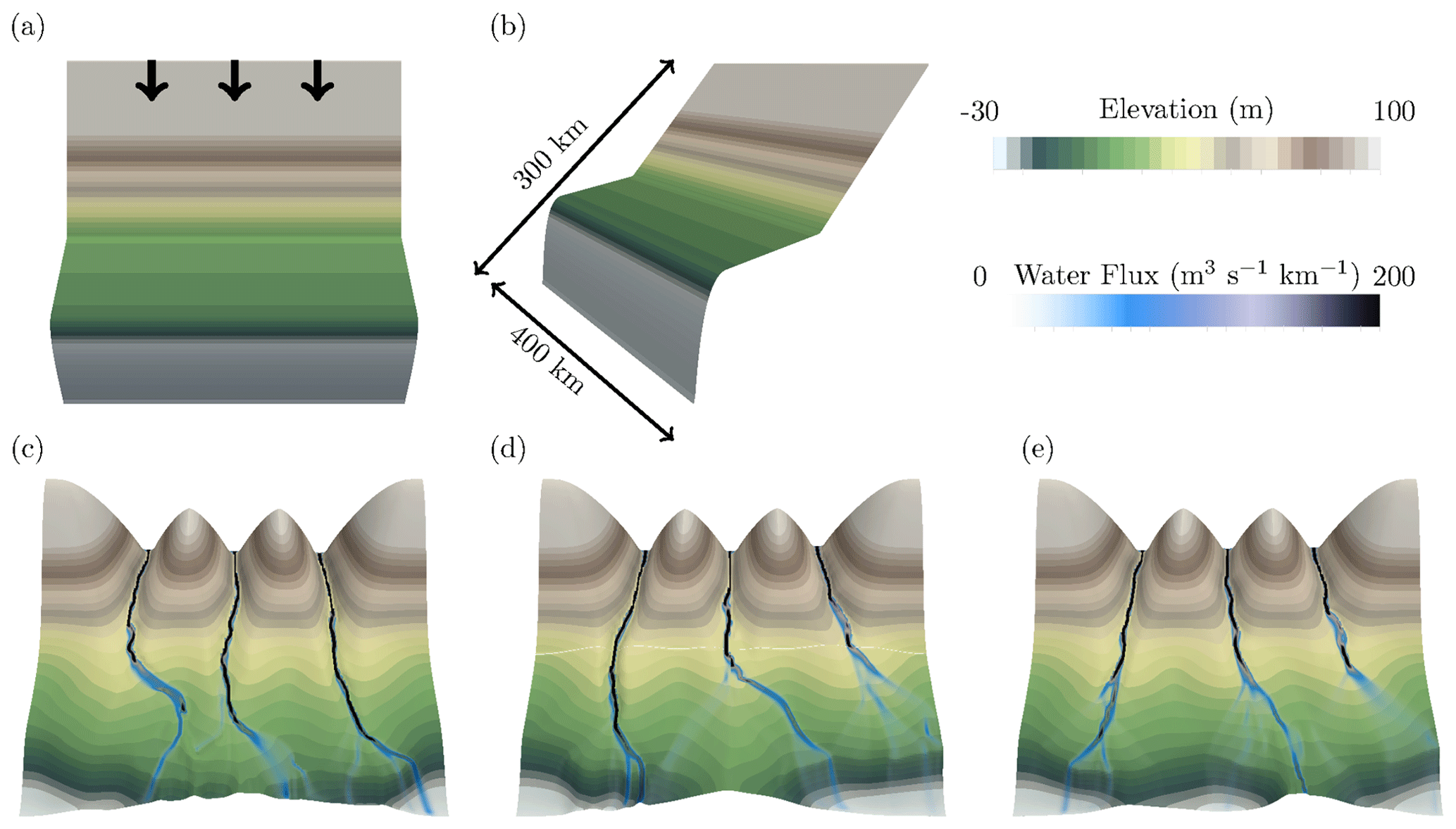
Figure 12 The “three rivers” test case with Δ_xy=2 km. (a, b) Initial topography; black arrows represent the position of the water inflows. (c–e) Topography and water flux after 6 Myr obtained under different numerical settings. (c) Sequential GMRES, (d) parallel GMRES, and (e) sequential BiCGStab.

An essential remark is that the whole configuration is symmetric with respect to the vertical plane $x=Lx/\mathrm{2}$. In principle, the equation system consisting of Eqs. (2) and (4), here used with r_s=2, p_s=1, should maintain this symmetry. Since we do not know the exact solution this time, at least we can use symmetry to identify erroneous results that do not fulfill this elementary requirement. Using the finite-volume scheme depicted in Appendix C, we perform a set of three identical simulations in terms of physical parameters but using different numerical settings in order to illustrate the impacts of numerical errors. We perform a sequential computation using GMRES as our linear solver for all systems, its parallel equivalent on four processors, and another sequential simulation using BiCGStab as our linear solver for all systems. The linear solvers are part of the well-known reference PETSc library (Balay et al., 1998) to avoid any potential mistake in their implementation, while the parallelism relies on the Arcane framework (Grospellier and Lelandais, 2009). Final topographies and water flux are shown in the bottom row of Fig. 12. Figure 12c corresponds to sequential GMRES, Fig. 12d to parallel GMRES, and Fig. 12e to sequential BiCGStab.

All the results from these simulations should be almost identical and in any case symmetrical with respect to the vertical plane $x=Lx/\mathrm{2}$ in the absence of any spatial heterogeneity in the input data. Clearly, symmetry is lost in the three cases, and what is even more striking is that we get three very different results. The only difference between the three cases being the numerical solvers, this indicates that it originates from numerical errors. As we are using a decoupled time scheme between water flow and sediment evolution (see Appendix C), one may argue that those instabilities are arising from some violated coupling constraint on the time step. Should this be the case, reducing the time step enough would ultimately lead to clean solutions. However, we have observed the exact opposite: the smaller the time step, the larger the obtained instabilities. The fact that reducing the time step makes things even worse is thus another clear sign that our problems are the result of amplified error accumulation up to the point that it influences flow branching.

4 Large structure simulation (LSS): an attempt to get rid of instabilities in LEMs

In this section, we explain how to transpose the ideas underlying the concept of large eddy simulation from the computational fluid dynamics community to our landscape evolution model. The method consists in preventing any self-amplification phenomena that might emerge from the small spatial scales where numerical errors develop. In our opinion, this is a key ingredient for achieving reproducible LEM simulations.

4.1 Principles and physical interpretation of filtering

Recall that the main idea of LES is to filter the solution to distinguish between the behavior of the flow above and below a target length scale α to obtain local averages that are smoother and as mesh-independent as possible. This target length scale controls the size of the smallest structures that we will be able to resolve in the problem, quite independently of the domain size. The main practical consequence is that our mesh will have to resolve this length scale; i.e., the mesh size ε will have to be smaller than the chosen length scale.

LES models are probably as numerous as the various authors working on the subject (Berselli et al., 2005); thus, we will be very brief on the subject and refer the reader to the recent review by Zhiyin (2015). The very first LES model is called the Leray-α model. It was used by Leray in 1934 to establish the existence of weak solutions to the Navier–Stokes equations (Leray, 1934). Originally, the filtering in Leray (1934) as well as in many classical LES models was achieved by using a convolution operator ℱ defined by

$$\mathcal{F}\left(u\right)\left(\mathit{x}\right)=\underset{{\mathbb{R}}^{\mathrm{d}}}{\int }u\left(\mathit{y}\right)g_{\mathit{\alpha }}(\mathit{x}-\mathit{y})\mathrm{d}\mathit{y},\mathrm{where}{g}_{\mathit{\alpha }}\left(\mathit{x}\right)={\displaystyle \frac{\mathrm{1}}{{\mathit{\alpha }}^{\mathrm{d}}}}g\left({\displaystyle \frac{\mathit{x}}{\mathit{\alpha }}}\right),$$

where the filter kernel g satisfies

$$\mathrm{0}\le g\left(\mathit{x}\right)\le \mathrm{1},g\left(\mathbf{0}\right)=\mathrm{1},\underset{{\mathbb{R}}^{\mathrm{d}}}{\int }g\left(\mathit{x}\right)\mathrm{d}\mathit{x}=\mathrm{1}.$$

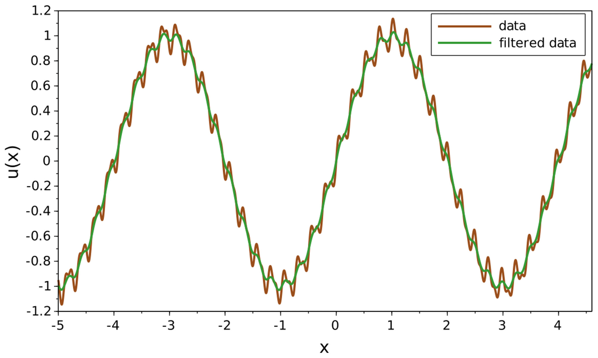
Several kernels are used in the literature, such as a low-pass filter, a box filter, or the very natural Gaussian filter $g\left(\mathit{x}\right)={\mathit{\pi }}^{-\mathrm{d}/\mathrm{2}}{e}^{-|\mathit{x}{|}^{\mathrm{2}}}$. In Fig. 13 we illustrate the smoothing effect of a Gaussian kernel on oscillating data: as expected, it preserves the high-amplitude and low-frequency oscillation while filtering out the high-frequency and low-amplitude oscillations. Such filters might therefore be ideal for our application to landscape evolution models: the small topographic perturbations will be cleaned out such that the flow routing will not be affected by it. Although convolution operators produce averages with the desired properties, they are impractical on bounded domains. The modern way of defining the Leray-α filter for bounded domains consists in using the differential filter ℱ_α defined by (Cheskidov et al., 2005; Guermond et al., 2003)

$$\begin{array}{}\text{(16)}& \left|\begin{array}{ll}-{\mathit{\alpha }}^{\mathrm{2}}\mathrm{\Delta }{\mathcal{F}}_{\mathit{\alpha }}\left(u\right)+{\mathcal{F}}_{\mathit{\alpha }}\left(u\right)=u& \mathrm{in}\mathrm{\Omega },\\ \mathrm{\nabla }{\mathcal{F}}_{\mathit{\alpha }}\left(u\right)\cdot \mathit{n}=\mathrm{0}& \mathrm{on}\partial {\mathrm{\Omega }}_{\mathcal{N}}\\ {\mathcal{F}}_{\mathit{\alpha }}\left(u\right)=\mathrm{0}& \mathrm{on}\partial {\mathrm{\Omega }}_{\mathcal{D}}\end{array}\right..\end{array}$$

The filtered result ℱ_α(u) basically amounts to a convolution of u by Green's function underlying Eq. (16), i.e., the filter applied to the Dirac distribution. Using a finite-volume scheme ℱ_α, this time we can easily obtain a discrete version ℱ_α,h, which is one of the main reasons why we have chosen to use this filter, along with its theoretical and practical success for CFD. Notice that contrary to Cheskidov et al. (2005) and Guermond et al. (2003), we use homogeneous Neumann and Dirichlet boundary conditions instead of periodic boundary conditions to simplify the treatment of the boundary. The main drawback of this choice is that our filter does not commute with differential operators. Resorting to only Dirichlet boundary conditions would have solved this issue, but from our numerical experiments we found that this can create boundary effects unless the chosen Dirichlet boundary condition is adapted to the filtered quantity. The Neumann choice avoids those difficulties without creating any practical issues, which has motivated our choice. For quantities such as the water flux for which Neumann everywhere is a more natural boundary condition, we introduce the alternative filter ${\mathcal{F}}_{\mathit{\alpha }}^{\mathcal{N}}$ with only Neumann boundary conditions:

$$\begin{array}{}\text{(17)}& \left|\begin{array}{ll}-{\mathit{\alpha }}^{\mathrm{2}}\mathrm{\Delta }{\mathcal{F}}_{\mathit{\alpha }}^{\mathcal{N}}\left(u\right)+{\mathcal{F}}_{\mathit{\alpha }}^{\mathcal{N}}\left(u\right)=u& \mathrm{in}\mathrm{\Omega },\\ \mathrm{\nabla }{\mathcal{F}}_{\mathit{\alpha }}^{\mathcal{N}}\left(u\right)\cdot \mathit{n}=\mathrm{0}& \mathrm{on}\partial \mathrm{\Omega }\end{array}\right..\end{array}$$

Figure 13 Illustration of the effect of the convolution by a Gaussian function.

4.2 Leray filtering applied to our landscape evolution model

Our numerical observations suggest that for large values of τ the model governing the simultaneous evolution of sediment and water is as intractable to solution as the Navier–Stokes system is for large Reynolds numbers. Consequently, mimicking the idea of large eddy simulation (LES) we will now apply filtering to key parts of our model problem to obtain a more numerically stable approximate model. This means that the sediment flux used in the mass conservation equations,

$$\left|\begin{array}{ll}\frac{\partial h_{\mathrm{s}}}{\partial t}+\mathrm{div}\left({\mathit{J}}_{\mathrm{s}}\right)=S_{\mathrm{s}}& \mathrm{in}\mathrm{\Omega }\times ]t_{\mathrm{0}},T[,\\ -{\mathit{J}}_{\mathrm{s}}\cdot \mathit{n}=B_{\mathrm{s}}& \mathrm{on}\partial {\mathrm{\Omega }}_{\mathcal{N}}\times ]t_{\mathrm{0}},T[,\\ h_{\mathrm{s}}=\mathrm{0}& \mathrm{on}\partial {\mathrm{\Omega }}_{\mathcal{D}}\times ]t_{\mathrm{0}},T[,\\ h_{\mathrm{s}}\left(t=t_{\mathrm{0}}\right)=h_{\mathrm{s},\mathrm{0}}& \mathrm{in}\mathrm{\Omega },\end{array}\right.$$

will now be given by

$$\begin{array}{}\text{(18)}& \begin{array}{rl}{\mathit{J}}_{\mathrm{s}}=& -{\mathit{\eta }}_{\mathrm{s}}\left(h_{\mathrm{s}}\right)s_{\mathrm{ref}}^{-p_{\mathrm{s}}}\left|\right|\mathrm{\nabla }\left(h_{\mathrm{s}}+b\right)|{|}^{p_{\mathrm{s}}}\left({\left({\displaystyle \frac{{\mathcal{F}}_{\mathit{\alpha }}^{\mathcal{N}}\left(q_{\mathrm{w}}\right)}{q_{\mathrm{ref}}}}\right)}^{r_{\mathrm{s}}}\right.\\ & \left.\mathrm{\nabla }{\mathit{\psi }}_{\mathrm{w}}\left(h_{\mathrm{s}}+b\right)+\mathrm{\nabla }{\mathit{\psi }}_{\mathrm{g}}\left(h_{\mathrm{s}}+b\right)\right)\mathrm{in}\mathrm{\Omega }\times ]t_{\mathrm{0}},T[,\end{array}\end{array}$$

where we use the filtered water flux magnitude ${\mathcal{F}}_{\mathit{\alpha }}^{\mathcal{N}}\left(q_{\mathrm{w}}\right)$ instead of directly using the water flux q_w. In the same way, in the water equations, we will now use the filtered topography ℱ_α(h_s+b) instead of the topography h_s+b, leading to

$$\begin{array}{}\text{(19)}& \left|\begin{array}{l}{\mathbf{Q}}_{\mathrm{w}}=-\frac{k_m{h}_{\mathrm{w}}{\mathit{\eta }}_{\mathrm{w}}\left(h_{\mathrm{w}}\right)}{s_{\mathrm{ref}}^{p_{\mathrm{w}}}}\left|\right|\mathrm{\nabla }\left({\mathcal{F}}_{\mathit{\alpha }}\right(h_{\mathrm{s}}+b\left)\right)\left|{|}^{p_{\mathrm{w}}}\mathrm{\nabla }\right({\mathcal{F}}_{\mathit{\alpha }}(h_{\mathrm{s}}+b)),\\ \mathrm{div}\left({\mathbf{Q}}_{\mathrm{w}}\right)=S_{\mathrm{w}}\text{ in }\mathrm{\Omega },\\ {\mathbf{Q}}_{\mathrm{w}}\cdot n=B_{\mathrm{w}}\text{ on }\partial {\mathrm{\Omega }}_{\mathrm{in}},\end{array}\right.\end{array}$$

with the associated water flux:

$$\begin{array}{}\text{(20)}& \begin{array}{rl}{q}_{\mathrm{w}}=& \left|\right|k_m{h}_{\mathrm{w}}{\mathit{\eta }}_{\mathrm{w}}\left(h_{\mathrm{w}}\right)s_{\mathrm{ref}}^{-p_{\mathrm{w}}}\left|\right|\mathrm{\nabla }\left({\mathcal{F}}_{\mathit{\alpha }}\left(h_{\mathrm{s}}+b\right)\right)|{|}^{p_{\mathrm{w}}}\\ & \mathrm{\nabla }\left({\mathcal{F}}_{\mathit{\alpha }}\left(h_{\mathrm{s}}+b\right)\right)\left|\right|.\end{array}\end{array}$$

Our so-called large structure simulation (LSS) for landscape evolution thus consists in solving Eqs. (2)–(18)–(19)–(20). The name “large structures” originates from the fact that since we use filtering in the coupling process, the water model does not see anymore topographic details that are smaller than α, and in the same way the sediment evolution is no longer influenced by water flow details smaller than α. We have thus abandoned the idea of resolving all the scales involved in the landscape evolution problem and will only try to simulate the large sedimentary and water structures, hence the name LSS: only structures several times larger than the filter resolution α will appear in the final result.

4.3 Numerical results with filtering

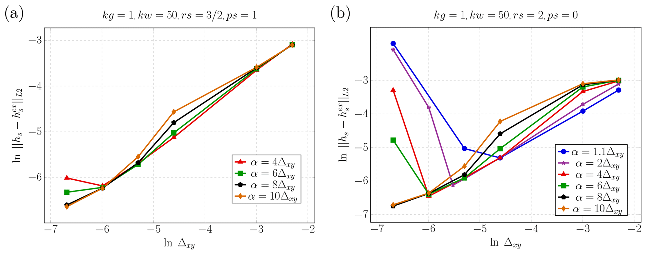
Before turning to numerical experiments, one must choose a value for the filter parameter α. Following LES principles, we know that the filter scale α corresponds to the spatial resolution of our continuous approximate model, which in practice one will want to be as small as possible. However, it must naturally be resolved by the grid, meaning we should have at the very least Δ_xy<α for Cartesian grids. Moreover, as we test our numerical solution against an analytic solution for the unfiltered case, we need to make the filter size go to zero at the same speed as the mesh size in order to measure a convergence. For simplicity, we have chosen to use filter parameters α=γΔ_xy with γ>1. In Fig. 14 we present the convergence results obtained for the analytic test cases of Sect. 3.1 this time using filters. Convergence is recovered with α=1.1Δ_xy (i.e., γ=1.1) for every case that was already working without a filter, suggesting that the LSS approach at least does not deteriorate correct results previously obtained. We also see that for the test cases with (k_g=1 km² Myr⁻¹, k_w=50 km² Myr⁻¹) convergence is now obtained for α=8Δ_xy (γ=8). This choice for the ratio γ between the filter size α and the mesh size Δ_xy is not random. Indeed, with α=γΔ_xy when Δ_xy tends to zero so does the filter size, and if γ is not large enough then the filtering parameter α will no longer be large enough to compensate for solver errors and numerical approximation errors. We illustrate this in Fig. 15. Keeping in mind that we are necessarily using a fixed Newton nonlinear solver tolerance ($\mathrm{1}\times {\mathrm{10}}^{-\mathrm{6}}$ in practice), what we observe on those curves is that when the parameter α becomes smaller than some threshold value that allows controlling the corresponding accumulated solver (and numerical approximation) errors, the obtained solution is no longer correct. Of course, with a larger value of γ this threshold is reached for a smaller value of Δ_xy, which explains why once γ is large enough we can obtain the correct solution along the entire convergence curve. This threshold is likely to depend on Δ_xy in the sense that for finer meshes since the size of the system is larger, so is the solver error. It is also very likely that since we expect larger values of τ to imply an increase in both the numerical approximation and solver errors, modifying τ might also influence this threshold value. Results shown in Fig. 15 confirm this behavior. This also explains why we have reported results with γ=8 in Fig. 14e: to maintain the convergence over the full range of Δ_xy values used for these simulations despite high τ values. We nevertheless see in Fig. 15 that for more realistic mesh sizes, smaller values of γ will be more than enough to obtain the correct solution and that using filters is not prohibitively costly in realistic configurations. We also observe that for mesh sizes allowing all the values of the ratio γ to give a correct approximation, the error of course increases with γ, which is perfectly expected since α is our largest approximation parameter.

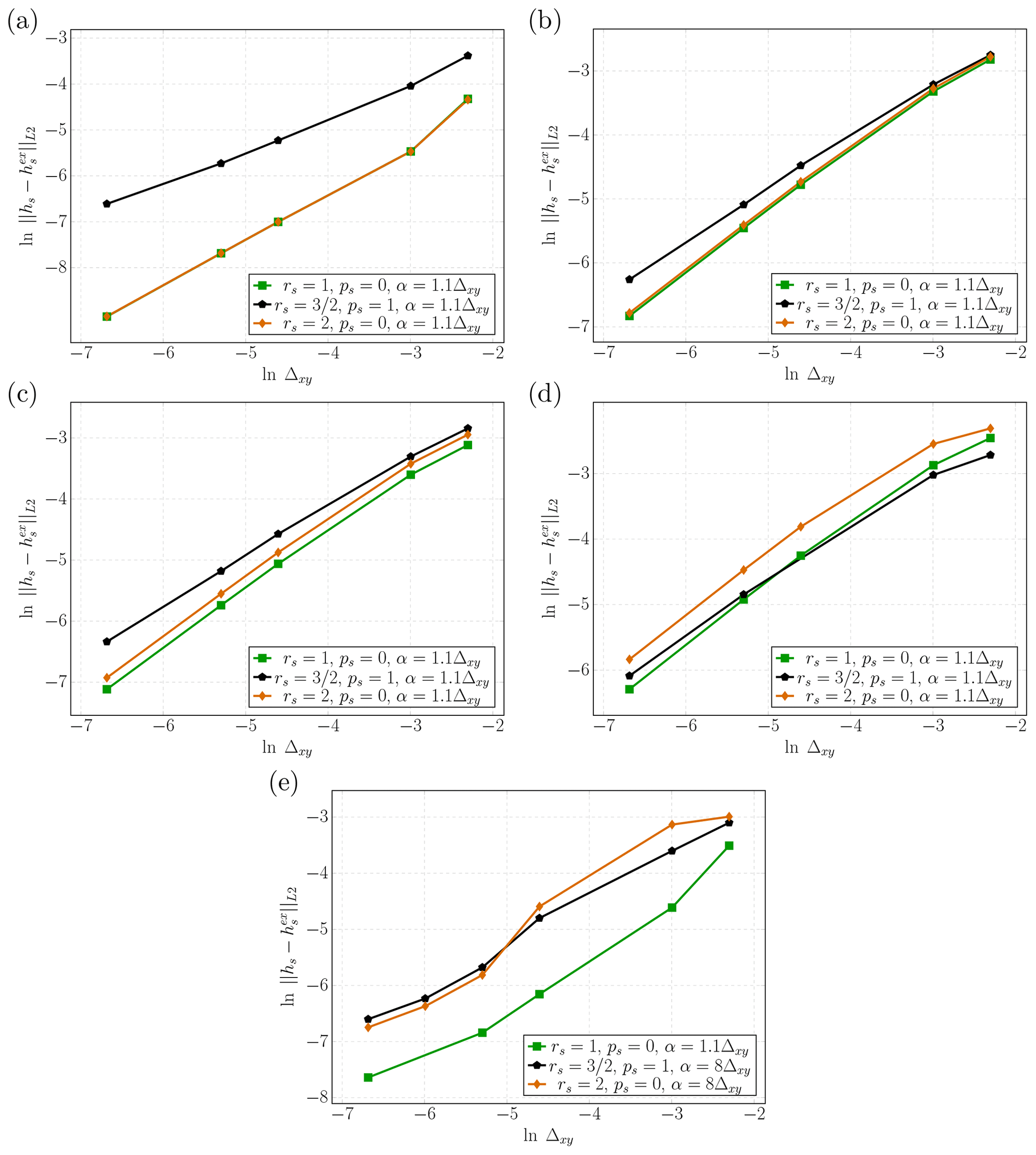
Figure 14 Convergence curves with filters. (a) Case k_g=50 km² Myr⁻¹ and k_w=1 km² Myr⁻¹. (b) Case k_g=5 km² Myr⁻¹ and k_w=1 km² Myr⁻¹. (c) Case k_g=5 km² Myr⁻¹ and k_w=5 km² Myr⁻¹. (d) Case k_g=1 km² Myr⁻¹ and k_w=5 km² Myr⁻¹. (e) Case k_g=1 km² Myr⁻¹ and k_w=50 km² Myr⁻¹.

Figure 15 Convergence curves for various values of the ratio $\mathit{\alpha }/{\mathrm{\Delta }}_{xy}$: (a) $(r_{\mathrm{s}},p_{\mathrm{s}})=(\mathrm{3}/\mathrm{2},\mathrm{1})$ and (b) $(r_{\mathrm{s}},p_{\mathrm{s}})=(\mathrm{2},\mathrm{0})$.

We finally reproduce the very same experiment that was performed on the “three rivers” test case with sequential GMRES, parallel GMRES, and sequential BiCGStab but using a filter α=2.2 km for Δ_xy=2 km. Contrary to Fig. 12, the symmetry is maintained and we obtain almost identical results for the three configurations (Fig. 16). The expected impact of the filter on the simulated water flow and topography is a smoothing effect, which is what is observed when comparing, for example, the width of the three valleys. However, the differences remain marginal in this case. Still on our “three rivers” test case, from our observations on the analytic cases and as we do not know the exact solution, to assess the legitimacy of our choice of filter size we analyze the behavior of the solution for various values of the filter parameter α (fixing the grid size to Δ_xy=2 km). Results are displayed in Fig. 17. We clearly see that symmetric solutions are obtained for α>Δ_xy, while further reducing the filter parameter leads to behavior similar to the no-filter case. This is first coherent with the principle of LES that the filter should control what happens below the grid scale, which can only be done if α>Δ_xy, and also a clear sign that our initial choice for the ratio $\mathit{\gamma }=\mathit{\alpha }/{\mathrm{\Delta }}_{xy}$ belongs to the stable region.

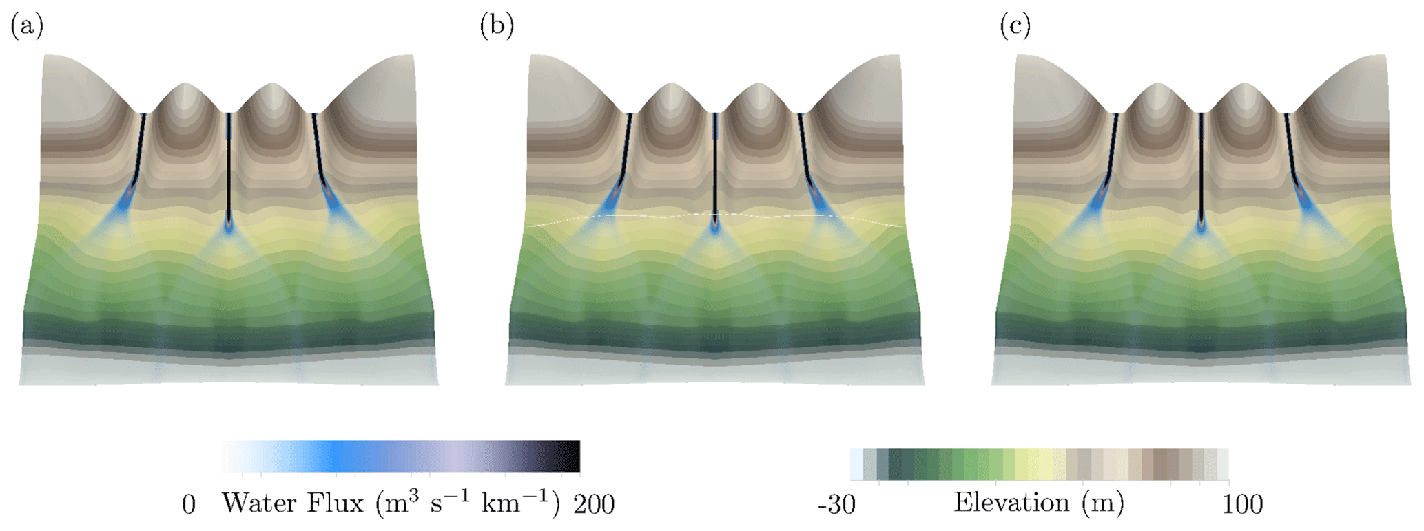
Figure 16 The “three rivers” test case with filter α=2.2 km and Δ_xy=2 km. Topography and water flux after 6 Myr. (a) Sequential GMRES, (b) parallel GMRES, and (c) sequential BiCGStab.

Figure 17 The “three rivers” test case with Δ_xy=2 km. Final topography and water flux after 6 Myr obtained with different values of the filter parameter α. (a) No filter, (b) α=0.2 km, (c) α=1 km, (d) α=2.2 km, (e) α=2.5 km, and (f) α=3 km.

The above results obtained with a filtering strategy represent, in our opinion, a drastic improvement in the reliability of these numerical solutions: the anomalous error amplification has disappeared, and the results are reproducible and unaffected by the choice of solver or the number of processors used for simulation. In the absence of this treatment, the error amplification phenomenon is most probably a great source of “anomalous mesh dependency” of the results as each mesh induces different numerical errors. The positive impact of our filtering strategy can be seen in the convergence curves (Fig. 15): it allows getting rid of any anomalous mesh dependency and recovering the regular one – that is to say when refining the mesh the associated sequence of solutions converges to the correct continuous solution. Notice that this is the best kind of “mesh independence” that one can hope for: in particular, quite large differences will remain when comparing two simulations defined on two different coarse meshes. Let us avoid any misunderstanding: the strategy prevents the amplification of numerical errors, but it does not clean the solution of legitimate numerical errors. This being said, we believe that following our approach brings us closer to the best possible mesh independence. When LEMs are designed without any filtering strategy, it corresponds to implicitly considering the mesh size as a cut-off length scale. However, it lacks calibration and leads to the error self-amplification problems illustrated in Sect. 3. In our case, we explicitly consider the filter size as a cut-off length scale, the resolution of the model being then controlled by the filter size. We will illustrate in the next sections that the calibration of this length must simply respect an elementary principle: to be largely lower that the size of the geomorphic structures the LEM aims to reproduce. Based on this calibration, the mesh resolution must be chosen so that the filter is correctly discretized. Thus, we have not deteriorated the overall computational situation: we still have a unique discretization parameter that governs the resolution and computational cost of the model.

4.4 Impacts of filtering on the emergence of geomorphic structures

We now consider two synthetic case studies to observe the formation of geomorphic features. The idea underlying the first test case is very simple: we re-use as our initial data the analytic solution described in Sect. 3.1 in the case (r_s=2, p_s=0) and (k_g=1 km² Myr⁻¹, k_w=50 km² Myr⁻¹) as well as the rectangular domain described in Fig. 3. However, instead of using the analytic source terms allowing the recovery of the analytic solution for all times, we simply use a constant source term (S_s=10 m Myr⁻¹, S_w=1 m³ s⁻¹ km⁻²), corresponding to a uniform constant uplift supply and a uniform constant rain.

We fix the mesh size to Δ_xy=0.005 km, and we again perform the simulation over a time period of 0.25 Myr with maximum time steps of length Δt=0.002 Myr. In Fig. 18, we recall the initial elevation corresponding to our analytic solution along with the final solution obtained for our now constant source terms for various values of the filter size as well as without filters. Since our new source terms and the analytic ones are of the same magnitude and since every other property of the problem is kept the same, we can guess, using the convergence curves in Fig. 15, which filter sizes are giving a correct solution (up to the approximation due to the filtering process itself). Since $\ln {\mathrm{\Delta }}_{xy}\approx -\mathrm{5.298}$, we see in Fig. 15 that for our choice of Δ_xy we can be confident that the filter size α=2Δ_xy will give us the correct solution with a small numerical approximation error, and we use this case as a reference. Thus, the first observation for the result obtained with α=2Δ_xy is that the correct solution this time allows some legitimate geomorphic structures to appear and self-organize. Those structures originate from the bumps because if we perform the very same simulation with constant source terms but without bumps, we obtain a clean uniform final state deprived of any geomorphic complexity. With the larger filter size α=4Δ_xy, we obtain an averaged version with slightly less geomorphic complexity, illustrating the way the filter only keeps “large” structures. However for the very large filter α=8Δ_xy the approximation for Δ_xy=0.005 km is too crude and we lose all the geomorphic complexity. We have checked that if we refine the mesh we recover the correct solution with the ratio α=8Δ_xy. This confirms that the uniform crude approximation obtained for α=8Δ_xy and Δ_xy=0.005 km in Fig. 18 results, as expected, from an oversizing of α. Now, let us consider the final solutions of Fig. 18 for the value α=1.1Δ_xy as well as without a filter. Both of those results present more complexity than the reference case α=2Δ_xy. Using the convergence curves of Fig. 15, we expect the result obtained for α=1.1Δ_xy to belong to the hazardous region where the error level starts to increase and this solution, while not completely erroneous, is becoming untrustworthy. However, for the solution without a filter strange small structures appear and the overall topography, despite being the most complex of all, does not have any physical origin.

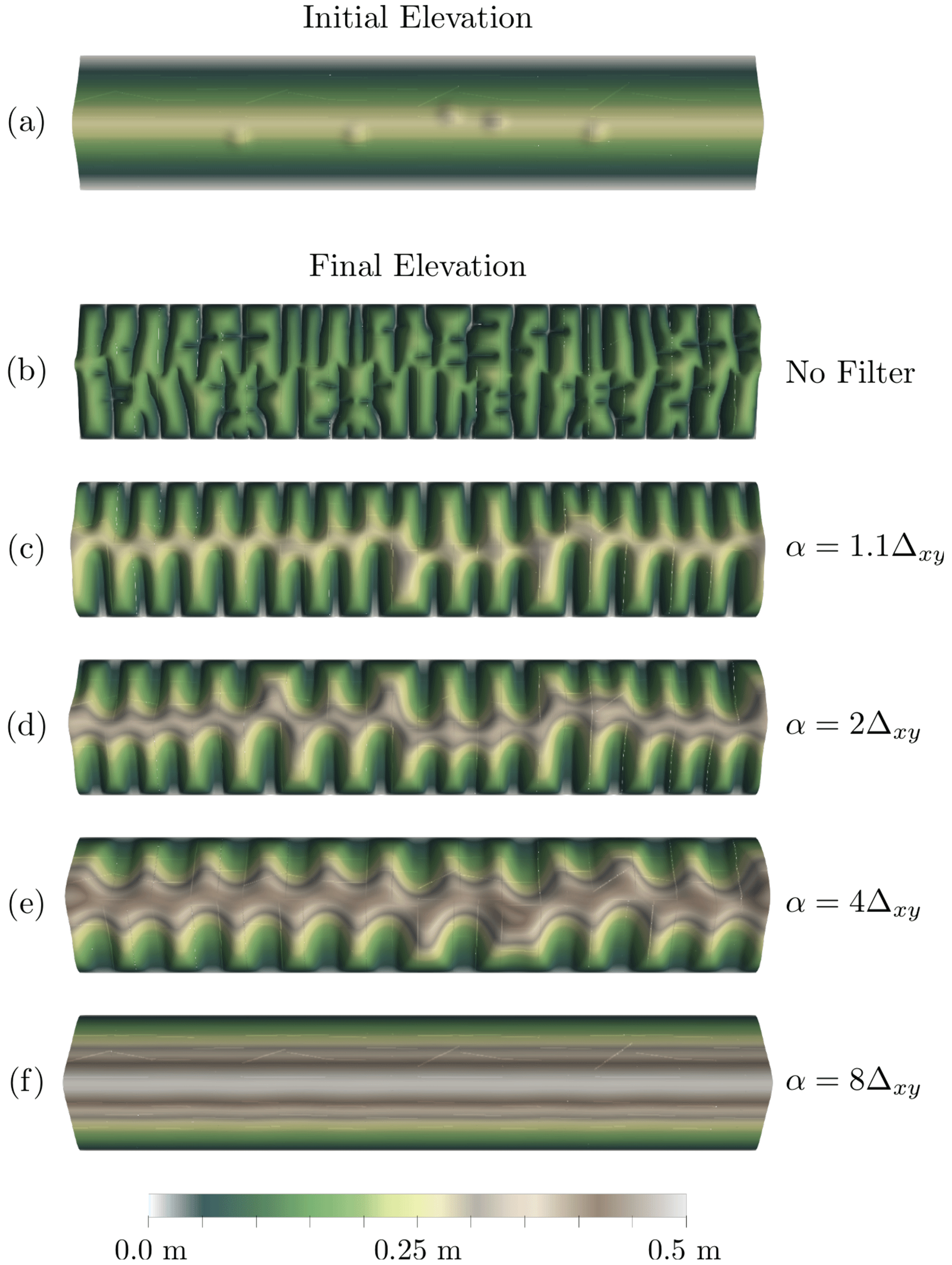
Figure 18 Results for a mesh size Δ_xy=0.005 km. (a) Initial elevation. Final elevation: (b) no filter, (c) α=1.1Δ_xy, (d) α=2Δ_xy, (e) α=4Δ_xy, (f) α=8Δ_xy.

We now switch to a second synthetic case study. The numerical domain again corresponds to a rectangular grid but this time with dimensions Lx=600 km on the x axis and Ly=80 km on the y axis containing a mesh of resolution Δ_xy=0.25 km. The basement b is constant and equal to 0 m, while the sediment thickness h_s is initially given by a uniform in x smooth bump:

$$g(x,y)=\left|\begin{array}{ll}H\exp \left(\frac{-\mathrm{1}}{\mathrm{1}-r_y^{\mathrm{2}}}\right)& \mathrm{for}{r}_y=\frac{\left(y-y_{\mathrm{c}}\right)}{{\mathit{\delta }}_y}\le \mathrm{1},\\ \mathrm{0}& \mathrm{otherwise},\end{array}\right.$$

with H=20 m, y_c=40 km, and δ_y=20 km. This symmetry in the x direction of the initial topography is then perturbed by N_b=30 small smooth bumps randomly positioned at points (x_p,y_p):

$$\begin{array}{ll}{\displaystyle }& {\displaystyle }{g}_{\mathrm{pert}}(x,y)=\\ {\displaystyle }& {\displaystyle }\left|\begin{array}{ll}{H}_{\mathrm{pert}}\exp \left(\frac{-\mathrm{1}}{\mathrm{1}-r^{\mathrm{2}}}\right)& \mathrm{for}{r}^{\mathrm{2}}=\frac{{\left(x-x_{\mathrm{p}}\right)}^{\mathrm{2}}}{{\mathit{\delta }}^{\mathrm{2}}}+\frac{{\left(y-y_{\mathrm{p}}\right)}^{\mathrm{2}}}{{\mathit{\delta }}^{\mathrm{2}}}\le \mathrm{1},\\ \mathrm{0}& \mathrm{otherwise},\end{array}\right.\end{array}$$

with H_pert=1 m and δ=2 km. Rainfall is constant in time and space (3000 mm yr⁻¹) and is the unique water supply for this case. The sediment source (here we simulate a sediment production) goes from S_s=0 m Myr⁻¹ at y=0 and y=Ly to S_s=100 m Myr⁻¹ at $y=Ly/\mathrm{2}=y_{\mathrm{c}}$. The variation is continuous over the whole domain following

$$S_{\mathrm{s}}(x,y)=\left|\begin{array}{ll}{S}_{\max }\exp \left(\frac{-\mathrm{1}}{\mathrm{1}-r_y^{\mathrm{2}}}\right)& \mathrm{for}{r}_y=\frac{\left(y-y_{\mathrm{c}}\right)}{{\mathit{\delta }}_y}\le \mathrm{1}\\ \mathrm{0}& \mathrm{otherwise},\end{array}\right.$$

with δ_y=40 km. Model boundary conditions are fixed elevations on the sides normal to the x axis and a zero gradient on the sides normal to the y axis. Model parameters controlling the nonlinearity in the water–sediment coupling are set as r_s=2 and p_s=0. Simulation takes place over the time period T=6 Myr.

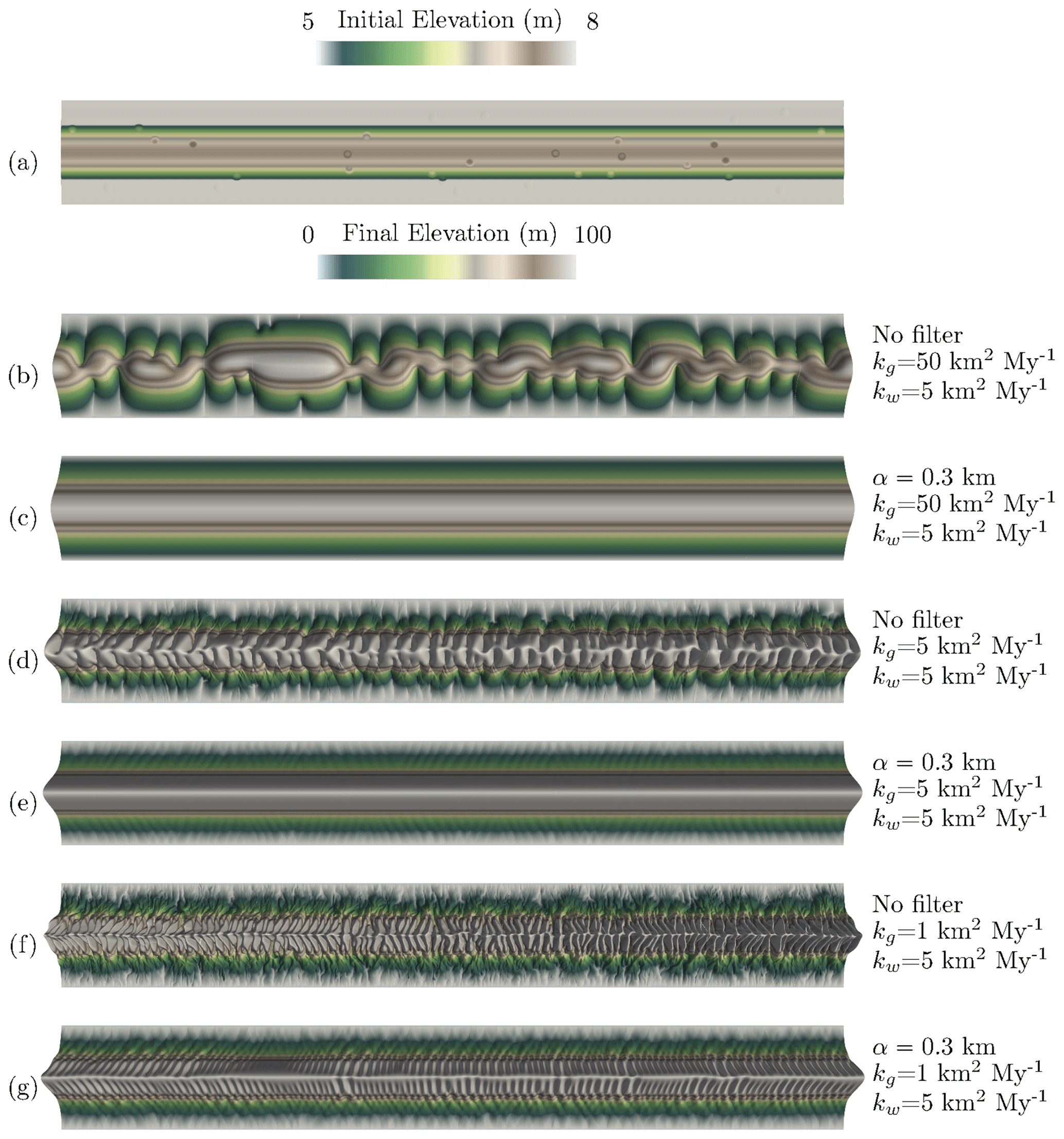
Figure 19 Final topographies obtained for three different set of diffusive coefficients, systematically tested without filter and with a filter using α=0.3 km. (a) Initial perturbed topography. (b) Solution without filter for $(k_{\mathrm{g}},k_{\mathrm{w}})=(\mathrm{50},\mathrm{5})$ km² Myr⁻¹, (c) solution with filter for $(k_{\mathrm{g}},k_{\mathrm{w}})=(\mathrm{50},\mathrm{5})$ km² Myr⁻¹, (d) solution without filter for $(k_{\mathrm{g}},k_{\mathrm{w}})=(\mathrm{5},\mathrm{5})$ km² Myr⁻¹, (e) solution with filter for $(k_{\mathrm{g}},k_{\mathrm{w}})=(\mathrm{5},\mathrm{5})$ km² Myr⁻¹, (f) solution without filter for $(k_{\mathrm{g}},k_{\mathrm{w}})=(\mathrm{1},\mathrm{5})$ km² Myr⁻¹, (g) solution with filter for $(k_{\mathrm{g}},k_{\mathrm{w}})=(\mathrm{1},\mathrm{5})$ km² Myr⁻¹.

This second synthetic case study has similarities to the previous one in terms of boundary conditions, but its larger spatial scale makes it relatively close to the case studies published in Perron et al. (2008) and Armitage (2019). We display the initial topography (Fig. 19a) as well as the final topography obtained with and without a filter for k_w=5 km² Myr⁻¹ and for three different k_g values. The first case considers k_g=50 km² Myr⁻¹. The relatively high k_g value compared to k_w should not favor the emergence of geomorphic structures. This is, however, not what we observe in the simulation performed without a filter (Fig. 19b). The filter, defined by α=0.3 km, has a huge impact and no geomorphic structure is produced (Fig. 19c). Refining both α and Δ_xy for this value of k_g, we always obtain the same uniform solution, which confirms that this is the correct one. An order of magnitude smaller k_g coefficient is used for the second simulation. By decreasing k_g, the emergence of structure may be considered a realistic result. In this case, complex structures controlled by at least one wavelength appear in the simulation performed without a filter (Fig. 19d). The effect of the filter, however, indicates the very likely artificial origin of these structures. A residual perturbation can still be observed in the final topography (Fig. 19e), indicating that this k_g and k_w configuration is at the transition between two regimes, the gravity-driven and the water-driven erosion regimes. In our last simulation, we have decreased k_g by a factor of 5 and we indeed observe the emergence of structures even when the filter is active (Fig. 19g). Here again the impact of the filter is important and allows keeping only what we believe to be the correct structures.

This last set of simulations shows the major impact of k_g on the wavelength of the structures that can emerge from our simulation. We have also performed additional simulations (not shown here) using various k_w values for a given k_g. The results show that k_w must be high enough to make the structures appear, but they also show that k_g was more important than k_w in the wavelength control. We believe that a dedicated study should be conducted with our model to quantify these effects, but it is beyond the scope of this article. Such a complete study can be found in Perron et al. (2008). Even if it was performed using another LEM, similar conclusions to those drawn from his study are also expected in our case.

5 Discussion

We consider this work to belong to the common effort of the scientific community to harmonize landscape evolution models. It is our belief that most of our observations and practical recommendations can also be applied to a wider range of sediment evolution models than the one we use in this study. The implementation of the large structure simulation strategy should be accessible to every LEM satisfying (H1), (H2), and (H3). In particular, we believe that filtering would also be very useful for the models of Perron et al. (2009), Hooshyar and Porporato (2021a), and Porporato (2022) that take the general form

$$\begin{array}{}\text{(21)}& \left|\begin{array}{ll}\frac{\partial h_{\mathrm{s}}}{\partial t}+\mathrm{div}\left({\mathit{J}}_{\mathrm{s}}\right)=S_{\mathrm{s}}& \mathrm{in}\mathrm{\Omega }\times ]t_{\mathrm{0}},T[,\\ -{\mathit{J}}_{\mathrm{s}}\cdot \mathit{n}=B_{\mathrm{s}}& \mathrm{on}\partial {\mathrm{\Omega }}_{\mathcal{N}}\times ]t_{\mathrm{0}},T[,\\ h_{\mathrm{s}}=\mathrm{0}& \mathrm{on}\partial {\mathrm{\Omega }}_{\mathcal{D}}\times ]t_{\mathrm{0}},T[,\\ h_{\mathrm{s}}\left(t=t_{\mathrm{0}}\right)=h_{\mathrm{s},\mathrm{0}}& \mathrm{in}\mathrm{\Omega },\end{array}\right.\end{array}$$

with a source given by

$$S_{\mathrm{s}}=U-{\mathit{\kappa }}_{\mathrm{w}}{s}_{\mathrm{ref}}^{-p_{\mathrm{s},\mathrm{2}}}{\left({\displaystyle \frac{q_{\mathrm{w}}}{q_{\mathrm{ref}}}}\right)}^{r_{\mathrm{s}}}\left|\right|\mathrm{\nabla }\left(h_{\mathrm{s}}+b\right)|{|}^{p_{\mathrm{s},\mathrm{2}}},$$

with U a sediment source term (or an uplift depending on the interpretation of b) and a sediment flux given by

$${\mathit{J}}_{\mathrm{s}}=-s_{\mathrm{ref}}^{-p_{\mathrm{s}}}{k}_{\mathrm{g}}\left|\right|\mathrm{\nabla }\left(h_{\mathrm{s}}+b\right)|{|}^{p_{\mathrm{s}}}\mathrm{\nabla }\left(h_{\mathrm{s}}+b\right)\mathrm{in}\mathrm{\Omega }\times ]t_{\mathrm{0}},T[.$$

The behavior of those models is relatively close to the model in Eqs. (2)–(9) that we have studied in detail here, with the main difference that the nonlinear term $q_{\mathrm{w}}^{r_{\mathrm{s}}}\left|\right|\mathrm{\nabla }(h_{\mathrm{s}}+b){|}^{p_{\mathrm{s}}}$ appears as a reaction term rather than a diffusive term. In particular, for $p_{\mathrm{w}}=-\mathrm{1}$ the observations of linear stability for the model in Eq. (21) match the conclusion of the linear stability analysis of Smith and Bretherton (1972) and Smith et al. (1997). We can thus expect that the model in Eq. (21) will potentially suffer from similar numerical stability issues to the ones we analyzed in detail for the model in Eqs. (2)–(9), although this certainly requires a dedicated study before drawing conclusions. In particular, several elements can help keep the numerical errors under control: high-order space and time schemes, explicit time schemes, and specific solvers for the water flow model avoiding inverting a linear system. Nevertheless, an immediate application of the LSS in this context consists of course of replacing q_w by its filtered version ${\mathcal{F}}_{\mathit{\alpha }}^{\mathcal{N}}\left(q_{\mathrm{w}}\right)$ in the second member of Eq. (21) and can only improve the numerical stability. We also believe that the ξ–q model of Davy and Lague (2009) could benefit from a similar filtering strategy.

Correctly using filters requires some understanding of the scales involved in the model. Although this is not such an easy task in general, from generic guidelines concerning the relation between the filter size α and the precision of the results it is clear that the chosen filtering parameter α should resolve the main sediment structures that one wants to correctly represent in the flow, ideally fulfilling an equivalent of Nyquist's rule. For instance, if an essential valley is 1 km large, then α should be several times smaller (and ideally smaller than 100 m). A good practical test consists in comparing the filtered topography ℱ_α(h_s+b) and the unfiltered one h_s+b. The structures of h_s+b that one wants to simulate accurately should be preserved in ℱ_α(h_s+b), of course in a smoother way. For instance, for a given value of α if a small topographic depression in which water could in principle flow is observed on h_s+b but is absent in ℱ_α(h_s+b), then if one really wants to capture water flow inside this “channel” the value of α must be reduced and the mesh refined accordingly if needed. The filter should in any case be able to clean numerical approximation and solver errors, implying that we should at the very least have $\mathit{\gamma }=\mathit{\alpha }/{\mathrm{\Delta }}_{xy}>\mathrm{1}$ to correctly resolve the targeted α spatial scale. To allow the filter to correctly clean errors that could otherwise have a destabilizing effect on the final configuration, higher values of α should probably be used for increasing values of τ. Nevertheless, our experiments illustrate that even quite small values of α allow cleaning the most relevant geomorphic features.

Notice that in the present paper, we have for simplicity always used uniform meshes with a constant Δ_xy, hence obtaining a constant ratio $\mathit{\gamma }=\mathit{\alpha }/{\mathrm{\Delta }}_{xy}$. As an immediate extension, one could resort to adaptive mesh refinement to refine the mesh in areas where τ becomes large and thus where numerical errors are more likely to be large, mitigating the increase in the system's size and thus the increase in the computational cost. In practice for constant coefficients k_g and k_w this would be equivalent to refining the mesh where water flow occurs. In addition, one could replace the constant parameter α by a space–time-variable coefficient $\mathit{\alpha }(x,y,t)$ in an adaptive filtering strategy, where the filter size could be chosen in coherence with the local size of the structures one wants the model to be able to reproduce.

5.1 Recovering realistic landscapes

In principle, the use of filters allows getting rid of the influence of numerical noise in the solution. An apparent drawback is that for unperturbed data, complex topographies will no longer appear by themselves through the perturbations induced by either the numerical approximation or the numerical solvers. Moreover, natural landscapes exhibit some heterogeneity even under a low-τ regime. This suggests an ingredient is missing, and this ingredient is well-known by geologists: the heterogeneity. Indeed heterogeneity is everywhere in nature and could be injected in such a model to make realistic-looking topographies emerge. This idea is of course not new but we propose investigating the effect of heterogeneity in the context of the hydro-sedimentary model we use for this paper.

We would also like to stress what is in our opinion an essential methodological key point: since natural landscapes are full of complex heterogeneities that are not contained in our data, it might be tempting to consider the amplified numerical noise as a way to recover the complexity lacking in our data. However, the statistical signature of numerical noise will never coincide with physical observations: it would be like throwing up the pieces of a puzzle and hoping that they will correctly reconstruct the puzzle while falling down. The key point is that a numerical simulation is not supposed to directly reproduce natural observations but only to compute a correct approximation of a model for a given dataset. This is the model and its data that should reproduce nature, and in this case if solved correctly the numerical solution will be a useful approximation. If we do not willingly add randomness in the data, the numerics should not introduce it out of nowhere and bypass our modeling: it is not reasonable to rely on numerical hazard to recover the missing elements in a model or its dataset. Worst of all, numerical noise lacks two essential modeling requirements: reproducibility and explainability. The first one is missing because numerical noise depends on the software and algorithms used and the number of processors, among other factors. The second one is missing because it is almost impossible to track how the numerical errors are generated.

The first heterogeneity we consider here is injected into the k_m coefficient, reflecting variable soil rugosity. Since acquiring a roughness map adapted to the spatial scales relevant to our approach is difficult and probably not relevant for a synthetic case study, we resort to an artificial yet efficient trick, namely the Perlin noise (Perlin, 1985) that is often used in animated movies or video games to produce realistic-looking mountains or river networks. This type of noise can easily be used to build isotropic heterogeneity maps with controlled spatial scales. We thus consider our “three rivers” test case using variable coefficients k_m in space and time (Fig. 20). Figure 20b illustrates a typical distribution in space of the k_m coefficients when using Perlin noise. The range of values for the k coefficient (from k_m=0.01 m s⁻¹ to k_m=10 m s⁻¹) is arbitrarily fixed while respecting realistic value ranges. Impacted by the heterogeneity in k_m, the water flow is still distributed between neighboring cells according to the gradient of the slope, but it also preferentially chooses to enter the cell with the highest k_m, especially when the slopes become gentle and relatively close between neighbors. The flow then acquires a high degree of complexity despite a filter which, set at α=1.1Δ_xy, makes it possible to eliminate numerical errors.

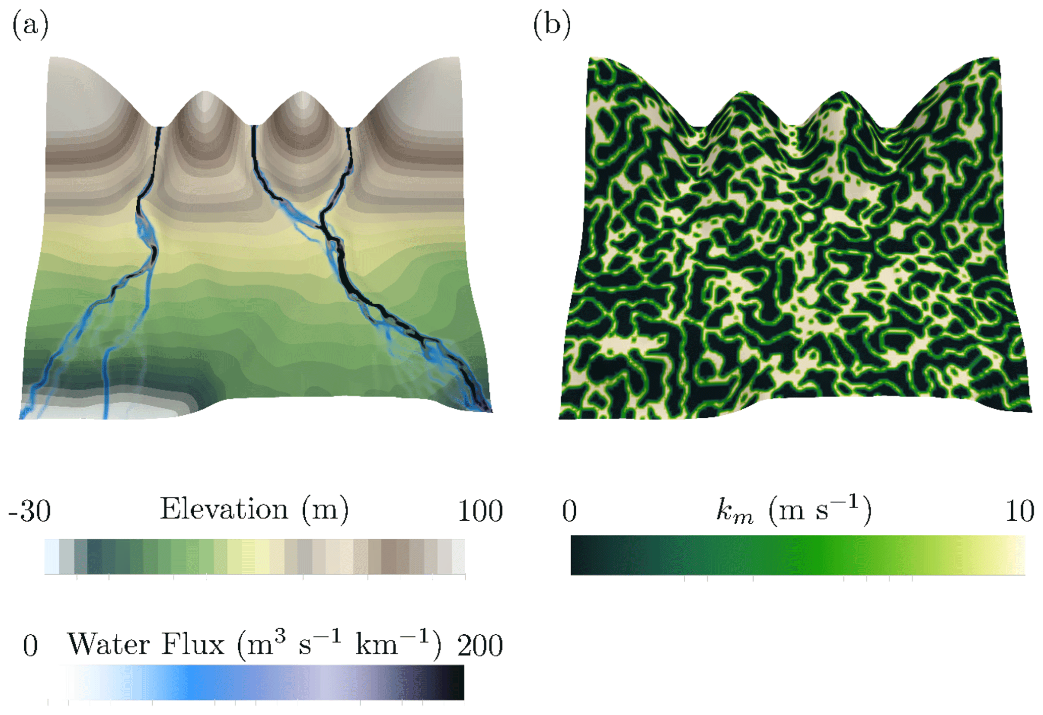
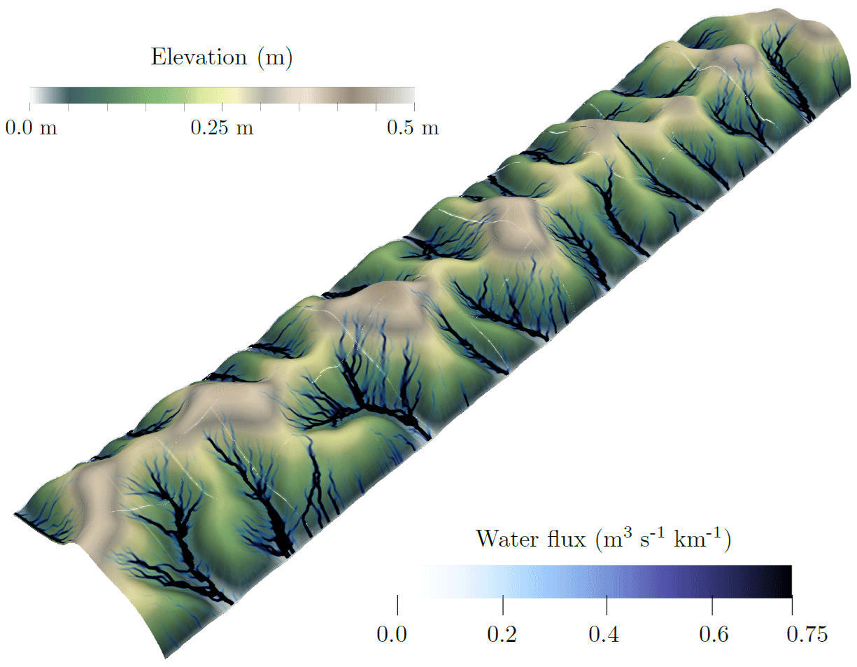
Figure 20 The “three rivers” test case with Perlin-noise-based coefficient k_m. (a) Final (at T=6 Myr) elevation and associated water flow with k_m coefficients variable in space and time. (b) k_m coefficients at T=6 Myr.

The same approach can be applied to the other synthetic test case used in Sect. 4.4 using α=2Δ_xy: the simulations are now performed with spatially and temporally varying k_m coefficients (the same range of k_m values is used). Figures 21a and b and 22 show the initial and the final state of the simulation with a special focus on the geomorphic structures produced, which are clearly more complex when comparing to the result shown in Fig. 18d.

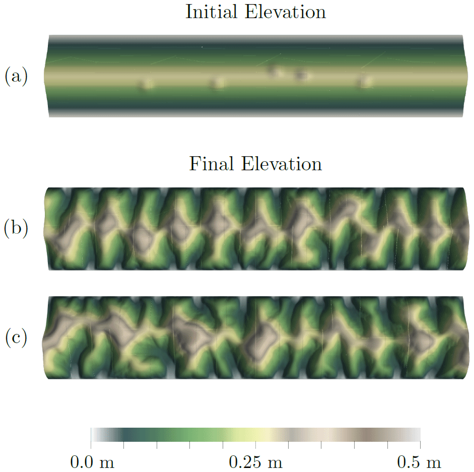
Figure 21 Results with filters and Perlin-noise-based k_m coefficient. (a) Initial elevation, (b) final elevation with variable coefficient k_m, and (c) final elevation with variable coefficient and additional Perlin-noise-based perturbation of rainfall.

Next, we introduce similar heterogeneity in the rain maps. When we use solely rain heterogeneity incorporating the same spatial scales as in the k_m maps, the geomorphic structures produced are very similar to those obtained using only the heterogeneous k_m coefficients. The most visually satisfying result is obtained for a simulation using both variable k_m and rain maps (Fig. 21c).

Figure 22 Front view of the result of Fig. 21c.

5.2 Overcoming the topographic limitations of the GMS model

The most obvious restriction for the GMS model in Eq. (4) to be well-posed is that the topography should not have any flat area; i.e., $\left|\right|\mathrm{\nabla }(h_{\mathrm{s}}+b)\left|\right|$ should not be identically zero on any measurable subset of Ω (subsets with nonzero area). Indeed, if $\left|\right|\mathrm{\nabla }(h_{\mathrm{s}}+b)\left|\right|=\mathrm{0}$ on 𝒪⊂Ω for p_w≥0 model in Eq. (4) becomes identically 0 on 𝒪, while for p_w<0 model in Eq. (4) (and thus also the model in Eq. 3) we have an under-determined form. In both situations, h_w and a cannot be computed on 𝒪. Arguably, true flat areas are rare for realistic topographies, however, a numerical algorithm can produce a few cells for which the topography is flat. A more common although less immediately obvious problem arises from accumulation areas. This is quite easy to understand: consider a bowl-shaped topography, with a flow of water coming from the boundary of only one half of the bowl. From the boundaries with inflow, all water will go straight down to the bottom of the bowl and stop there, since the flow can only progress if it finds a downhill direction. Water will remain stuck at the bottom and will never flow in the second half of the bowl. Since the models in Eqs. (4) and (3) correspond to steady-state water models this implies an infinite value for h_w at the bottom of the bowl. To put this into more mathematical terms with a very simple example, let us consider the model in Eq. (4) in the simplified setting where k_w=1, p_w=0 S_w=0, and $h_{\mathrm{s}}(x,y,t)+b(x,y,t)=x^{\mathrm{2}}+y^{\mathrm{2}}$ on the unit disk $\mathrm{\Omega }=\mathit{\left\{}\right(x,y)\in {\mathbb{R}}^{\mathrm{2}}|x^{\mathrm{2}}+y^{\mathrm{2}}<\mathrm{1}\mathit{\}}$. The model in Eq. (4) becomes

$$\begin{array}{ll}{\displaystyle }-\mathrm{div}\left(h_{\mathrm{w}}\mathrm{\nabla }\left(h_{\mathrm{s}}+b\right)\right)& {\displaystyle }=-\mathrm{\nabla }{h}_{\mathrm{w}}\cdot \mathrm{\nabla }\left(h_{\mathrm{s}}+b\right)-h_{\mathrm{w}}\mathrm{\Delta }\left(h_{\mathrm{s}}+b\right)\\ {\displaystyle }& {\displaystyle }=-\mathrm{2}x{\partial }_x{h}_{\mathrm{w}}-\mathrm{2}y{\partial }_y{h}_{\mathrm{w}}-\mathrm{4}{h}_{\mathrm{w}}=\mathrm{0},\end{array}$$

leading to solutions of the form $h_{\mathrm{w}}(x,y,t)=\frac{C}{(x+y{)}^{\mathrm{2}}}$. Assume that the boundary influx is given by B_w=1 for y≥0 and B_w=0 otherwise. Then, in the half-domain y≥0 we get h_w>0 with $h_{\mathrm{w}}⟶+\mathrm{\infty }$ when $(x,y⟶(\mathrm{0},\mathrm{0})$, which is unphysical. In the half-domain y<0, h_w=0 and q_w=0. This illustrates the two problems: infinite values for the water height and a water flux that abruptly stops on the line y=0.

This is reflected at the discrete level by an abrupt stop of the water flow at the bottom of accumulation areas. Moreover, this prevents recomputing a correct approximation of h_w or a from the intermediate unknown used in MFD algorithms (the total outflow of a cell), since the coefficient relating this intermediate unknown to h_w or a will be zero (see Coatléven, 2020, or Appendix C for details). This coefficient also cancels on flat areas. We can infer that this is a discrete indicator of what could be the weakest theoretical requirements on the topography for the models in Eqs. (3) and (4) to be well-posed: the absence of flat or accumulation areas.

Figure 23 Comparison of the models in Eqs. (4) and (22) on the “three rivers” test case for α=2.2 km and Δ_xy=2 km.

The model in Eq. (4) being in fact a simplification of the shallow-water equation (see Sect. 5.2), this limitation can be seen as the price to pay to simulate the water flow mass conservation with a very low computational expense. At the cost of a higher computational time alternative models also derived from the shallow-water equation can be considered to overcome this limitation (see Sect. 5.2). Notice that in the following numerical experiments, we have been careful to only consider situations for which no well-posedness issues occur.

In the general setting, there is no reason why the sediments should evolve in such a way that one of the sufficient conditions in Eq. (8) is always fulfilled, which can lead to some nonphysical behavior of the GMS model in Eq. (4) and thus also the pure MFD algorithms. This can occur in two obvious situations: in an accumulation area (a topographic depression) or a flat area. In principle, water arriving at an accumulation area should create a “lake” whose bathymetry will be determined by a water balance between incoming flow, infiltration, and evaporation. If the surface reaches the threshold of the lake, then some water leaves the lake and the water flow restarts from the lake threshold. In flat areas, water will spread, diminishing its height until the full area is covered. To reproduce those effects that are not originally considered, implementations of the MFD algorithms all incorporate practical workarounds. Thanks to our interpretation as the discretization of a continuous model, we can easily propose a generalization of Eq. (4) that overcomes those limitations by noticing that the model in Eq. (4) is in fact a simplification of the shallow-water equations with friction. Indeed, appropriately choosing the friction model and assuming that the mass conservation of water is at steady state, a quite general model arising from applying the hydrostatic approximation to the shallow-water equations would be to consider (see Appendix B)

$$\begin{array}{}\text{(22)}& \left|\begin{array}{l}{\mathbf{Q}}_{\mathrm{w}}=-\frac{k_m{h}_{\mathrm{w}}{\mathit{\eta }}_{\mathrm{w}}\left(h_{\mathrm{w}}\right)}{s_{\mathrm{ref}}^{p_{\mathrm{w}}}}\left|\right|\mathrm{\nabla }(h_{\mathrm{w}}+h_{\mathrm{s}}+b)\left|{|}^{p_{\mathrm{w}}}\mathrm{\nabla }\right(h_{\mathrm{w}}+h_{\mathrm{s}}+b),\\ \mathrm{div}\left({\mathbf{Q}}_{\mathrm{w}}\right)=S_{\mathrm{w}}\text{ in }\mathrm{\Omega },\\ {\mathbf{Q}}_{\mathrm{w}}\cdot n=B_{\mathrm{w}}\text{ on }\partial {\mathrm{\Omega }}_{\mathcal{N}},\\ h_{\mathrm{w}}=\mathrm{0}\text{ on }\partial {\mathrm{\Omega }}_{\mathcal{D}},\end{array}\right.\end{array}$$

with the associated water flux strength:

$$\begin{array}{}\text{(23)}& q_{\mathrm{w}}=\left|k_m{h}_{\mathrm{w}}{\mathit{\eta }}_{\mathrm{w}}\left(h_{\mathrm{w}}\right)\right|s_{\mathrm{ref}}^{-p_{\mathrm{w}}}\left|\right|\mathrm{\nabla }\left(h_{\mathrm{w}}+h_{\mathrm{s}}+b\right)|{|}^{p_{\mathrm{w}}+\mathrm{1}}.\end{array}$$

This is almost Eq. (4) except that it uses the hydraulic gradient instead of the topographic one.The assumption $\mathrm{\nabla }(h_{\mathrm{s}}+b)\approx \mathrm{\nabla }(h_{\mathrm{w}}+h_{\mathrm{s}}+b)$, while valid on pronounced slopes, is obviously not valid anymore in accumulation areas (at equilibrium, the hydraulic gradient is almost zero, while the topographic gradient is large) and flat areas (where the topographic gradient is zero and the hydraulic one is not). The nonlinear model in Eq. (22) is thus a natural generalization of the GMS model in Eq. (4) with a built-in handling of accumulation and flat areas which no longer requires practical workarounds. However, the model in Eq. (22) does come with some drawbacks. The first one is that now we must choose the water mobility function η_w, as we are solving for the water height unknown. This will influence both the water network and the strength of the water flow. In the same way, the absolute value of the coefficient k_m will now impact the strength of the water flux through h_w, while only its contrasts were relevant for the GMS model in Eq. (4). Thus, some fine tuning is required for Eq. (22) to produce meaningful results. The last and probably more important drawback is that, Eq. (22) being nonlinear in its unknown h_w, its discretization will be more involved and computationally expensive than for Eq. (4). Let us compare the results obtained with the original GMS model in Eq. (4) with the more involved hydrologic model in Eq. (22) on the “three rivers” test case using filters in both cases. The water mobility function η_w for Eq. (22) is simply chosen as equal to 1 if h_w is positive and 0 otherwise.

As we can observe in Fig. 23, if the two models of course do not produce exactly the same results, their general behavior remains very similar. Even more close results could certainly be obtained by finely tuning the mobility function. We do not want to explore this any further in the present paper and simply want to illustrate that while suffering from some limitations, the GMS model in Eq. (4) and thus MFD algorithms remain a very strong and attractive approximation on suitable topographies.

6 Conclusions

After illustrating the numerical instabilities arising from the self-amplification phenomenon at the core of coupling overland flow and sediment evolution models, we have proposed mimicking the LES strategy for CFD computation in the context of landscape evolution models, relying on the well-known Leray-α differential filter. Numerical experiments assess whether filtering produces results robust to numerical perturbations. It is our belief that this “large structure simulation” (LSS) approach goes far beyond the specific model considered here and that any LEMs involving a coupling with surface water flow could benefit from it. Indeed, experiments performed without any filtering strategy have shown that it can become extremely difficult to distinguish between the imprint of numerical errors and physical processes. Provided suitable filter parameters and mesh sizes are used, only the nonphysical heterogeneity will disappear. The size of the filter has a real modeling meaning and corresponds to the minimum size of the physical heterogeneity that can be resolved. The choice of its value depends mainly on the accuracy required, which of course also depends on the computational power. Deploying this technique in a geomorphic model that has incorporated the correct water flux expression will make it possible to correct the anomalous mesh dependency so often evoked in papers dealing with LEM behavior. Indeed, if LEMs are designed to reproduce complex emergent phenomena arising from a set of simple physical processes and data, they are in no way intended to give a physical meaning to non-reproducible numerical noise, even if this noise once amplified by physical processes leads to “good-looking” results. The apparently missing visual complexity that previously arose from numerical noise can be physically re-introduced when heterogeneous data are considered. Similarly to LES models, we believe that a mathematical analysis and numerical analysis of the filtered model should be achievable. We hope to be able to publish such an analysis in a future paper. To complete this work, we also plan to use in our next study the full model capacity in building a multi-lithology realistic test case. Finally, pursuing the analogy with LES, an interesting perspective would be to analyze whether it is feasible to develop subfilter models to increase the filtered model accuracy when α is quite large in order to reduce the need for fine α and thus fine meshes and consequently the overall cost of the approach.

Appendix A: Computational details related to perturbation theory

Recall that we denote ($h_{\mathrm{s},*},h_{\mathrm{w},*}$) a reference solution of Eqs. (2)–(9)–(4) with sources ($S_{\mathrm{s},*},S_{\mathrm{w},*}$) and ($h_{\mathrm{s},\mathit{\delta }},h_{\mathrm{w},\mathit{\delta }}$), a perturbation of magnitude δ of this reference solution associated with the source perturbation ($S_{\mathrm{s},\mathit{\delta }},S_{\mathrm{w},\mathit{\delta }}$), leading to the overall solution ($h_{\mathrm{s}},h_{\mathrm{w}})=(h_{\mathrm{s},*}+h_{\mathrm{s},\mathit{\delta }},h_{\mathrm{w},*}+h_{\mathrm{w},\mathit{\delta }}$) for the perturbed source ($S_{\mathrm{s},*}+S_{\mathrm{s},\mathit{\delta }},S_{\mathrm{w},*}+S_{\mathrm{w},\mathit{\delta }}$). Since both the perturbed and unperturbed solutions have to satisfy the boundary conditions, we deduce that the perturbation ($h_{\mathrm{s},\mathit{\delta }},h_{\mathrm{w},\mathit{\delta }}$) itself also satisfies the same boundary conditions. Thus, injecting (h_s,h_w) into Eqs. (2)–(9), multiplying by h_s,δ, and integrating by parts we get

$$\begin{array}{}\text{(A1)}& \begin{array}{rl}{\displaystyle \frac{\mathrm{d}}{\mathrm{d}t}}& \left({\displaystyle \frac{\mathrm{1}}{\mathrm{2}}}\underset{\mathrm{\Omega }}{\int }{h}_{\mathrm{s},\mathit{\delta }}^{\mathrm{2}}\right)=-\underset{\mathrm{\Omega }}{\int }{\mathit{\eta }}_{\mathrm{s}}\left(h_{\mathrm{s}}\right)s_{\mathrm{ref}}^{-p_{\mathrm{s}}}\left|\right|\mathrm{\nabla }\left(h_{\mathrm{s}}+b\right)|{|}^{p_{\mathrm{s}}}\\ & \left({\left({\displaystyle \frac{q_{\mathrm{w}}}{q_{\mathrm{ref}}}}\right)}^{r_{\mathrm{s}}}{k}_{\mathrm{w}}+k_{\mathrm{g}}\right)\left|\right|\mathrm{\nabla }{h}_{\mathrm{s},\mathit{\delta }}|{|}^{\mathrm{2}}+\underset{\mathrm{\Omega }}{\int }{\mathit{\eta }}_{\mathrm{s}}\left(h_{\mathrm{s},*}\right)s_{\mathrm{ref}}^{-p_{\mathrm{s}}}\\ & \left|\right|\mathrm{\nabla }\left(h_{\mathrm{s},*}+b\right)|{|}^{p_{\mathrm{s}}}\left({\left({\displaystyle \frac{q_{\mathrm{w},*}}{q_{\mathrm{ref}}}}\right)}^{r_{\mathrm{s}}}{k}_{\mathrm{w}}+k_{\mathrm{g}}\right)\mathrm{\nabla }\left(h_{\mathrm{s},*}+b\right)\\ & \cdot \mathrm{\nabla }{h}_{\mathrm{s},\mathit{\delta }}-\underset{\mathrm{\Omega }}{\int }{\mathit{\eta }}_{\mathrm{s}}\left(h_{\mathrm{s}}\right)s_{\mathrm{ref}}^{-p_{\mathrm{s}}}\left|\right|\mathrm{\nabla }\left(h_{\mathrm{s}}+b\right)|{|}^{p_{\mathrm{s}}}\left({\left({\displaystyle \frac{q_{\mathrm{w}}}{q_{\mathrm{ref}}}}\right)}^{r_{\mathrm{s}}}\right.\\ & \left.k_{\mathrm{w}}+k_{\mathrm{g}}\right)\mathrm{\nabla }\left(h_{\mathrm{s},*}+b\right)\cdot \mathrm{\nabla }{h}_{\mathrm{s},\mathit{\delta }}+\underset{\mathrm{\Omega }}{\int }{S}_{\mathrm{s},\mathit{\delta }}{h}_{\mathrm{s},\mathit{\delta }}.\end{array}\end{array}$$

When denoting

$$\begin{array}{}\text{(A2)}& j_{\mathrm{s}}(u,v,w)={\mathit{\eta }}_{\mathrm{s}}\left(u\right)s_{\mathrm{ref}}^{-p_{\mathrm{s}}}\left|\right|\mathrm{\nabla }v|{|}^{p_{\mathrm{s}}}\left({\left({\displaystyle \frac{w}{q_{\mathrm{ref}}}}\right)}^{r_{\mathrm{s}}}{k}_{\mathrm{w}}+k_{\mathrm{g}}\right),\end{array}$$

we recover the claimed equation governing the evolution of the perturbation's total energy:

$$\begin{array}{}\text{(A3)}& \begin{array}{rl}{\displaystyle \frac{d}{dt}}& \left({\displaystyle \frac{\mathrm{1}}{\mathrm{2}}}\underset{\mathrm{\Omega }}{\int }{h}_{\mathrm{s},\mathit{\delta }}^{\mathrm{2}}\right)=-\underset{\mathrm{\Omega }}{\int }{j}_{\mathrm{s}}\left(h_{\mathrm{s}},h_{\mathrm{s}}+b,q_{\mathrm{w}}\right)\left|\right|\mathrm{\nabla }{h}_{\mathrm{s},\mathit{\delta }}|{|}^{\mathrm{2}}\\ & +\underset{\mathrm{\Omega }}{\int }{S}_{\mathrm{s},\mathit{\delta }}{h}_{\mathrm{s},\mathit{\delta }}+\underset{\mathrm{\Omega }}{\int }\left(j_{\mathrm{s}}\left(h_{\mathrm{s},*},h_{\mathrm{s},*}+b,q_{\mathrm{w},*}\right)\right.\\ & \left.-j_{\mathrm{s}}\left(h_{\mathrm{s}},h_{\mathrm{s}}+b,q_{\mathrm{w}}\right)\right)\mathrm{\nabla }\left(h_{\mathrm{s},*}+b\right)\cdot \mathrm{\nabla }{h}_{\mathrm{s},\mathit{\delta }}.\end{array}\end{array}$$

Then, if k_g is much larger than k_w and thus τ is very small, we have, assuming for simplicity that η_s=1 from Taylor's expansion,

$$\begin{array}{}\text{(A4)}& \begin{array}{rl}{A}_{\mathit{\delta }}& \approx k_{\mathrm{g}}{s}_{\mathrm{ref}}^{-p_{\mathrm{s}}}\left(\left|\right|\mathrm{\nabla }\left(h_{\mathrm{s},*}+b\right)|{|}^{p_{\mathrm{s}}}-|\left|\mathrm{\nabla }\left(h_{\mathrm{s}}+b\right)\right|{|}^{p_{\mathrm{s}}}\right)\\ & \mathrm{\nabla }\left(h_{\mathrm{s},*}+b\right)\cdot \mathrm{\nabla }{h}_{\mathrm{s},\mathit{\delta }}+O\left(\mathit{\tau }\right)\approx -k_{\mathrm{g}}{s}_{\mathrm{ref}}^{-p_{\mathrm{s}}}\\ & \left(p_{\mathrm{s}}\left|\right|\mathrm{\nabla }\left(h_{\mathrm{s},*}+b\right)\left|{|}^{p_{\mathrm{s}}-\mathrm{2}}\right|\mathrm{\nabla }\left(h_{\mathrm{s},*}+b\right)\cdot \mathrm{\nabla }{h}_{\mathrm{s},\mathit{\delta }}{|}^{\mathrm{2}}\right)\\ & +O\left(\mathit{\tau }\right)+O\left({\mathit{\delta }}^{\mathrm{3}}\right).\end{array}\end{array}$$

In the same way, if k_w is much larger than k_g then τ is also very large and we have, again using Taylor's expansion,

$$\begin{array}{}\text{(A5)}& \begin{array}{rl}{A}_{\mathit{\delta }}& \approx -k_{\mathrm{w}}{s}_{\mathrm{ref}}^{-p_{\mathrm{s}}}{q}_{\mathrm{ref}}^{-r_{\mathrm{s}}}\left(q_{\mathrm{w},*}^{r_{\mathrm{s}}}\left|\right|\mathrm{\nabla }\left(h_{\mathrm{s},*}+b\right)|{|}^{p_{\mathrm{s}}}-q_{\mathrm{w}}^{r_{\mathrm{s}}}||\right.\\ & \left.\mathrm{\nabla }\left(h_{\mathrm{s}}+b\right)|{|}^{p_{\mathrm{s}}}\right)\mathrm{\nabla }\left(h_{\mathrm{s},*}+b\right)\cdot \mathrm{\nabla }{h}_{\mathrm{s},\mathit{\delta }}+O(\mathrm{1}/\mathit{\tau })\\ & \approx -k_{\mathrm{w}}{s}_{\mathrm{ref}}^{-p_{\mathrm{s}}}{r}_{\mathrm{s}}{\displaystyle \frac{q_{\mathrm{w},*}^{r_{\mathrm{s}}-\mathrm{1}}}{q_{\mathrm{ref}}^{r_{\mathrm{s}}}}}{q}_{\mathrm{w},\mathit{\delta }}\left|\right|\mathrm{\nabla }\left(h_{\mathrm{s},*}+b\right)|{|}^{p_{\mathrm{s}}}\mathrm{\nabla }\left(h_{\mathrm{s},*}+b\right)\\ & \cdot \mathrm{\nabla }{h}_{\mathrm{s},\mathit{\delta }}-k_{\mathrm{w}}{s}_{\mathrm{ref}}^{-p_{\mathrm{s}}}{\left({\displaystyle \frac{q_{\mathrm{w},*}}{q_{\mathrm{ref}}}}\right)}^{r_{\mathrm{s}}}\left(p_{\mathrm{s}}\left|\right|\mathrm{\nabla }\left(h_{\mathrm{s},*}+b\right)\left|{|}^{p_{\mathrm{s}}-\mathrm{2}}\right|\right.\\ & \left.\mathrm{\nabla }\left(h_{\mathrm{s},*}+b\right)\cdot \mathrm{\nabla }{h}_{\mathrm{s},\mathit{\delta }}{|}^{\mathrm{2}}\right)+O(\mathrm{1}/\mathit{\tau })+O\left({\mathit{\delta }}^{\mathrm{3}}\right).\end{array}\end{array}$$

Going back to the general case for η_s, we have for small values of τ

$$\begin{array}{}\text{(A6)}& \begin{array}{rl}{A}_{\mathit{\delta }}& \approx -k_{\mathrm{g}}{s}_{\mathrm{ref}}^{-p_{\mathrm{s}}}\left({\mathit{\eta }}_{\mathrm{s}}^{\prime }\left(h_{\mathrm{s},*}\right)\left|\right|\mathrm{\nabla }\left(h_{\mathrm{s},*}+b\right)|{|}^{p_{\mathrm{s}}}{h}_{\mathrm{s},\mathit{\delta }}\right.\\ & \left.\mathrm{\nabla }\left(h_{\mathrm{s},*}+b\right)\cdot \mathrm{\nabla }{h}_{\mathrm{s},\mathit{\delta }}+p_{\mathrm{s}}{\mathit{\eta }}_{\mathrm{s}}\left(h_{\mathrm{s},*}\right)\left|\right|\mathrm{\nabla }\left(h_{\mathrm{s},*}\right)+b\right)\left|{|}^{p_{\mathrm{s}}-\mathrm{2}}\right|\\ & \left.\mathrm{\nabla }\left(h_{\mathrm{s},*}+b\right)\cdot \mathrm{\nabla }{h}_{\mathrm{s},\mathit{\delta }}{|}^{\mathrm{2}}\right)+O\left(\mathit{\tau }\right)+O\left({\mathit{\delta }}^{\mathrm{3}}\right),\end{array}\end{array}$$

while for large values of τ we have

$$\begin{array}{}\text{(A7)}& \begin{array}{rl}{A}_{\mathit{\delta }}& \approx -k_{\mathrm{w}}{s}_{\mathrm{ref}}^{-p_{\mathrm{s}}}{r}_{\mathrm{s}}{\displaystyle \frac{q_{\mathrm{w},*}^{r_{\mathrm{s}}-\mathrm{1}}}{q_{\mathrm{ref}}^{r_{\mathrm{s}}}}}{q}_{\mathrm{w},\mathit{\delta }}{\mathit{\eta }}_{\mathrm{s}}\left(h_{\mathrm{s},*}\right)\left|\right|\mathrm{\nabla }\left(h_{\mathrm{s},*}+b\right)|{|}^{p_{\mathrm{s}}}\\ & \mathrm{\nabla }\left(h_{\mathrm{s},*}+b\right)\cdot \mathrm{\nabla }{h}_{\mathrm{s},\mathit{\delta }}-k_{\mathrm{w}}{s}_{\mathrm{ref}}^{-p_{\mathrm{s}}}{\left({\displaystyle \frac{q_{\mathrm{w},*}}{q_{\mathrm{ref}}}}\right)}^{r_{\mathrm{s}}}\left({\mathit{\eta }}_{\mathrm{s}}^{\prime }\left(h_{\mathrm{s},*}\right)\right.\\ & \left|\right|\mathrm{\nabla }\left(h_{\mathrm{s},*}+b\right)|{|}^{p_{\mathrm{s}}}{h}_{\mathrm{s},\mathit{\delta }}\mathrm{\nabla }\left(h_{\mathrm{s},*}+b\right)\cdot \mathrm{\nabla }{h}_{\mathrm{s},\mathit{\delta }}\\ & +p_{\mathrm{s}}{\mathit{\eta }}_{\mathrm{s}}\left(h_{\mathrm{s},*}\right)\left|\right|\mathrm{\nabla }\left(h_{\mathrm{s},*}+b\right)\left|{|}^{p_{\mathrm{s}}-\mathrm{2}}\right|\mathrm{\nabla }\left(h_{\mathrm{s},*}+b\right)\\ & \left.\cdot \mathrm{\nabla }{h}_{\mathrm{s},\mathit{\delta }}{|}^{\mathrm{2}}\right)+O(\mathrm{1}/\mathit{\tau })+O\left({\mathit{\delta }}^{\mathrm{3}}\right).\end{array}\end{array}$$

The behavior is roughly speaking the same, with the main difference that the additional term in ${\mathit{\eta }}_{\mathrm{s}}^{\prime }\left(h_{\mathrm{s},*}\right)$ can also contribute with the wrong sign. Since ${\mathit{\eta }}_{\mathrm{s}}^{\prime }\left(h_{\mathrm{s},*}\right)$ will be almost zero as soon as $h_{\mathrm{s},*}$ is large enough (see Eq. 11), this can only happen in regions where $h_{\mathrm{s},*}$ is close to zero (in particular near Dirichlet boundaries). In this case, the potential contribution to the instabilities is controlled by the magnitude of $\left|{\mathit{\eta }}_{\mathrm{s}}^{\prime }\right(h_{\mathrm{s},*}\left)h_{\mathrm{s},\mathit{\delta }}\right|\le \left|h_{\mathrm{s},\mathit{\delta }}\right|/h_{\mathrm{c}}$. If the perturbation is not amplified by other engines, which will be the case if τ is small, and if the parameter h_c is not chosen to be too small (a typical valid value is 20 cm), then no severe instability can occur through this additional term. Thus, we can be confident that parameter τ will be the main criterion governing the appearance of instabilities even for our most general model.

Appendix B: From shallow-water model to the steady-state hydrologic model in Eq. (22)

Recall that the shallow-water system is given by (see Birnir et al., 2001; Peton et al., 2020)

$$\begin{array}{}\text{(B1)}& \left|\begin{array}{l}\frac{\partial h_{\mathrm{w}}}{\partial t}+\mathrm{div}\left(h_{\mathrm{w}}{\mathbf{u}}_{\mathrm{w}}\right)=\mathrm{0},\\ {\displaystyle \frac{\partial }{\partial t}}\left(h_{\mathrm{w}}{\mathbf{u}}_{\mathrm{w}}\right)+\mathrm{div}(h_{\mathrm{w}}{\mathit{u}}_{\mathrm{w}}\otimes {\mathbf{u}}_{\mathrm{w}})+g{h}_{\mathrm{w}}\mathrm{\nabla }(h_{\mathrm{s}}+b+h_{\mathrm{w}})+\\ =-{\mathit{\kappa }}_{\mathrm{w}}\left(h_{\mathrm{w}},\left|\right|\mathrm{\nabla }(h_w+h_{\mathrm{s}}+b)\left|\right|\right)|{\mathbf{u}}_{\mathrm{w}}{|}^{r_{\mathrm{w}}}{\mathbf{u}}_{\mathrm{w}},\end{array}\right.\end{array}$$

where u_w denotes the water speed, g is the acceleration due to gravity, and κ_w is the friction coefficient. Then, following Peton et al. (2020) and defining H_s,c to be the characteristic sediment height, H_w,c the characteristic water height, L_c the characteristic domain length, and T_c the characteristic time, as well as defining the nondimensional variables,

$$\begin{array}{ll}{\displaystyle }{\widehat{h}}_{\mathrm{s}}=& {\displaystyle \frac{h_{\mathrm{s}}}{H_{\mathrm{s},\mathrm{c}}}},{\widehat{b}}_{\mathrm{s}}={\displaystyle \frac{b}{H_{\mathrm{s},\mathrm{c}}}},{\widehat{h}}_{\mathrm{w}}={\displaystyle \frac{h_{\mathrm{w}}}{H_{\mathrm{w},\mathrm{c}}}},{\widehat{\mathit{u}}}_{\mathrm{w}}={\displaystyle \frac{T_{\mathrm{c}}{\mathit{u}}_{\mathrm{w}}}{L_{\mathrm{c}}}},\\ {\displaystyle }& {\displaystyle }\widehat{x}={\displaystyle \frac{x}{L_{\mathrm{c}}}},\widehat{y}={\displaystyle \frac{y}{L_{\mathrm{c}}}},\widehat{t}={\displaystyle \frac{t}{T_{\mathrm{c}}}},\end{array}$$

we see that Eq. (B1) is equivalent to

$$\left|\begin{array}{l}\frac{\partial {\widehat{h}}_{\mathrm{w}}}{\partial \widehat{t}}+\widehat{\mathrm{div}}\left({\widehat{h}}_{\mathrm{w}}{\widehat{\mathit{u}}}_{\mathrm{w}}\right)=\mathrm{0},\\ {\displaystyle \frac{\partial }{\partial \widehat{t}}}\left({\widehat{h}}_{\mathrm{w}}{\widehat{\mathit{u}}}_{\mathrm{w}}\right)+\widehat{\mathrm{div}}({\widehat{h}}_{\mathrm{w}}{\widehat{\mathit{u}}}_{\mathrm{w}}\otimes {\widehat{\mathit{u}}}_{\mathrm{w}})\\ +g{\displaystyle \frac{H_{\mathrm{s},\mathrm{c}}{T}_{\mathrm{c}}^{\mathrm{2}}}{L_{\mathrm{c}}^{\mathrm{2}}}}{\widehat{h}}_{\mathrm{w}}\widehat{\mathrm{\nabla }}({\widehat{h}}_{\mathrm{s}}+\widehat{b})+g{\displaystyle \frac{H_{\mathrm{w},\mathrm{c}}{T}_{\mathrm{c}}^{\mathrm{2}}}{L_{\mathrm{c}}^{\mathrm{2}}}}{\widehat{h}}_{\mathrm{w}}\widehat{\mathrm{\nabla }}\left({\widehat{h}}_{\mathrm{w}}\right),\\ =-{\mathit{\kappa }}_{\mathrm{w}}\left(h_{\mathrm{w}},\left|\right|\mathrm{\nabla }(h_{\mathrm{w}}+h_{\mathrm{s}}+b)\left|\right|\right){\displaystyle \frac{L_{\mathrm{c}}}{H_{\mathrm{w},\mathrm{c}}}}{\left({\displaystyle \frac{L_{\mathrm{c}}}{T_{\mathrm{c}}}}\right)}^{r_{\mathrm{w}}-\mathrm{1}}|{\widehat{\mathit{u}}}_{\mathrm{w}}{|}^{r_{\mathrm{w}}}{\widehat{\mathit{u}}}_{\mathrm{w}}.\end{array}\right.$$

The “shallow” hypothesis corresponds to assuming that $L_{\mathrm{c}}/H_{\mathrm{w},\mathrm{c}}\gg \mathrm{1}$, while the two numbers

$$F_{\mathrm{r},\mathrm{w}}={\displaystyle \frac{L_{\mathrm{c}}}{\sqrt{g{H}_{\mathrm{w},\mathrm{c}}}{T}_{\mathrm{c}}}}\mathrm{and}{F}_{\mathrm{r},\mathrm{s}}={\displaystyle \frac{L_{\mathrm{c}}}{\sqrt{g{H}_{\mathrm{s},\mathrm{c}}}{T}_{\mathrm{c}}}}$$

are equivalent to Froude numbers for the water and sediment flows. For long-term sediment evolution, it is reasonable to assume that $F_{\mathrm{r},\mathrm{w}}\ll \mathrm{1}$ and $F_{\mathrm{r},\mathrm{s}}\ll \mathrm{1}$, i.e., that gravity is the dominant phenomenon. Combined with the shallow-water assumption this suggests neglecting the inertia terms in the nondimensional momentum balance, leading to the hydrostatic assumption:

$$\begin{array}{}\text{(B2)}& \begin{array}{rl}g{h}_{\mathrm{w}}\mathrm{\nabla }\left(h_{\mathrm{s}}+b+h_{\mathrm{w}}\right)=& -{\mathit{\kappa }}_{\mathrm{w}}\left(h_{\mathrm{w}},\left|\right|\mathrm{\nabla }\left(h_{\mathrm{w}}+h_{\mathrm{s}}+b\right)\left|\right|\right)\\ & |{\mathit{u}}_{\mathrm{w}}{|}^{r_{\mathrm{w}}}{\mathit{u}}_{\mathrm{w}}.\end{array}\end{array}$$

Inverting Eq. (B2) we obtain the following expression for the water speed:

$$\begin{array}{}\text{(B3)}& {\mathit{u}}_{\mathrm{w}}=-{\mathit{\mu }}_{\mathrm{w}}\left(h_{\mathrm{w}},\left|\right|\mathrm{\nabla }\left(h_{\mathrm{w}}+h_{\mathrm{s}}+b\right)\left|\right|\right)\mathrm{\nabla }\left(h_{\mathrm{s}}+b+h_{\mathrm{w}}\right),\end{array}$$

where

$$\begin{array}{}\text{(B4)}& \begin{array}{rl}{\mathit{\mu }}_{\mathrm{w}}& \left(h_{\mathrm{w}},\left|\right|\mathrm{\nabla }\left(h_{\mathrm{w}}+h_{\mathrm{s}}+b\right)\left|\right|\right)\\ & ={\displaystyle \frac{g^{\frac{\mathrm{1}}{r_{\mathrm{w}}+\mathrm{1}}}{h}_{\mathrm{w}}^{\frac{\mathrm{1}}{r_{\mathrm{w}}+\mathrm{1}}}}{{\mathit{\kappa }}_{\mathrm{w}}{\left(h_{\mathrm{w}},\left|\right|\mathrm{\nabla }\left(h_{\mathrm{w}}+h_{\mathrm{s}}+b\right)\left|\right|\right)}^{\frac{\mathrm{1}}{r_{\mathrm{w}}+\mathrm{1}}}}}\\ & \left|\right|\mathrm{\nabla }\left(h_{\mathrm{s}}+b+h_{\mathrm{w}}\right)|{|}^{-\frac{r_{\mathrm{w}}}{r_{\mathrm{w}}+\mathrm{1}}}.\end{array}\end{array}$$

Thus, appropriately choosing the friction model, for instance by setting r_w=0 and

$$\begin{array}{}\text{(B5)}& \begin{array}{rl}{\mathit{\kappa }}_{\mathrm{w}}& \left(h_{\mathrm{w}},\left|\right|\mathrm{\nabla }\left(h_{\mathrm{w}}+h_{\mathrm{s}}+b\right)\left|\right|\right)\\ & ={\displaystyle \frac{g{h}_{\mathrm{w}}}{k_m{\mathit{\eta }}_{\mathrm{w}}\left(h_{\mathrm{w}}\right)s_{\mathrm{ref}}^{-p_{\mathrm{w}}}\left|\right|\mathrm{\nabla }\left(h_{\mathrm{w}}+h_{\mathrm{s}}+b\right)|{|}^{p_{\mathrm{w}}}}},\end{array}\end{array}$$

and assuming that the mass conservation of water is at steady state, we obtain the following quite general hydrostatic approximation to the shallow-water equations:

$$\left|\begin{array}{l}{\mathbf{Q}}_{\mathrm{w}}=-\frac{k_m{h}_{\mathrm{w}}{\mathit{\eta }}_{\mathrm{w}}\left(h_{\mathrm{w}}\right)}{s_{\mathrm{ref}}^{p_{\mathrm{w}}}}\left|\right|\mathrm{\nabla }(h_{\mathrm{w}}+h_{\mathrm{s}}+b)\left|{|}^{p_{\mathrm{w}}}\mathrm{\nabla }\right(h_{\mathrm{w}}+h_{\mathrm{s}}+b),\\ \mathrm{div}\left({\mathbf{Q}}_{\mathrm{w}}\right)=S_{\mathrm{w}}\text{ in }\mathrm{\Omega },\\ {\mathbf{Q}}_{\mathrm{w}}\cdot n=B_{\mathrm{w}}\text{ on }\partial {\mathrm{\Omega }}_{\mathcal{N}},\\ h_{\mathrm{w}}=\mathrm{0}\text{ on }\partial {\mathrm{\Omega }}_{\mathcal{D}},\end{array}\right.$$

with the associated water flux strength:

$$q_{\mathrm{w}}=\left|k_m{h}_{\mathrm{w}}{\mathit{\eta }}_{\mathrm{w}}\left(h_{\mathrm{w}}\right)\right|s_{\mathrm{ref}}^{-p_{\mathrm{w}}}\left|\right|\mathrm{\nabla }\left(h_{\mathrm{w}}+h_{\mathrm{s}}+b\right)|{|}^{p_{\mathrm{w}}+\mathrm{1}}.$$

Remark B.1. The friction model in Eq. (B5) becomes singular when $\left|\right|\mathrm{\nabla }(h_{\mathrm{w}}+h_{\mathrm{s}}+b)\left|\right|=\mathrm{0}$. Thus, an alternative choice would be to use something like

$$\begin{array}{ll}{\displaystyle }{\mathit{\kappa }}_{\mathrm{w}}& {\displaystyle }\left(h_{\mathrm{w}},\left|\right|\mathrm{\nabla }\left(h_{\mathrm{w}}+h_{\mathrm{s}}+b\right)\left|\right|\right)\\ {\displaystyle }& {\displaystyle }={\displaystyle \frac{g{h}_{\mathrm{w}}}{k_m{\mathit{\eta }}_{\mathrm{w}}\left(h_{\mathrm{w}}\right)\left(\mathit{\beta }+s_{\mathrm{ref}}^{-p_{\mathrm{w}}}\left|\right|\mathrm{\nabla }\left(h_{\mathrm{w}}+h_{\mathrm{s}}+b\right)|{|}^{p_{\mathrm{w}}}\right)}}\end{array}$$

for some β>0 (the same holds for function η_w such that η(0)=0). This alternative choice is probably more physical, as the term in $s_{\mathrm{ref}}^{-p_{\mathrm{w}}}\left|\right|\mathrm{\nabla }(h_{\mathrm{w}}+h_{\mathrm{s}}+b)|{|}^{p_{\mathrm{w}}}$ can be interpreted as modeling some deceleration in accumulation areas. We have chosen to use Eq. (B5) to be as close as possible to the MFD algorithms of the literature.

Appendix C: Finite-volume discretization

In this section we describe the full finite-volume discretization of the system in Eqs. (2)–(18)–(19)–(20). Let Ω be a bounded polyhedral connected domain of ℝ², whose boundary is denoted as $\partial \mathrm{\Omega }=\stackrel{\mathrm{‾}}{\mathrm{\Omega }}\setminus \mathrm{\Omega }$. We recall the usual finite-volume notations describing a mesh $\mathcal{M}=(\mathcal{T},\mathcal{F})$ of Ω. The set of the cells of the mesh 𝒯 is a finite family of connected open disjoint polygonal subsets of Ω such that $\stackrel{\mathrm{‾}}{\mathrm{\Omega }}={\cup }_{K\in \mathcal{T}}\stackrel{\mathrm{‾}}{K}$. For any K∈𝒯, we denote $\left|K\right|$ the measure of K, $\partial K=\stackrel{\mathrm{‾}}{K}\setminus K$ the boundary of K, ρ_K its diameter, and x_K its barycenter. The set of faces of the mesh ℱ is a finite family of disjoint subsets of ℝ² included in $\stackrel{\mathrm{‾}}{\mathrm{\Omega }}$ such that, for all σ∈ℱ, its measure is denoted $\left|\mathit{\sigma }\right|$, its diameter h_σ, and its barycenter x_σ. For any K∈𝒯, the faces of cells K correspond to the subset ℱ_K of ℱ such that $\partial K={\cup }_{\mathit{\sigma }\in {\mathcal{F}}_K}\stackrel{\mathrm{‾}}{\mathit{\sigma }}$. Then, for any face σ∈ℱ, we denote ${\mathcal{T}}_{\mathit{\sigma }}=\mathit{\{}K\in \mathcal{T}|\mathit{\sigma }\in {\mathcal{F}}_K\mathit{\}}$ the cells of which σ is a face. Next, for all cell K∈𝒯 and all face σ∈ℱ_K of cell K, we denote n_K,σ the unit normal vector to σ outward to K, and $d_{K,\mathit{\sigma }}=|{\mathit{x}}_{\mathit{\sigma }}-{\mathit{x}}_K|$. The set of boundary faces is denoted ℱ_ext, while interior faces are denoted ℱ_int. Finally for any σ∈ℱ_int, whenever the context is clear we will denote K and L the two cells forming ${\mathcal{T}}_{\mathit{\sigma }}=\mathit{\{}K,L\mathit{\}}$, as well as $d_{KL}=|{\mathit{x}}_K-{\mathit{x}}_L|$. This, for instance, allows when looping over the faces σ of cell K denoting L the other face of σ without resorting to a notation that is too heavy. To avoid any confusion with water and sediment heights, $\mathit{ϵ}={\max }_{K\in \mathcal{T}}{\mathit{\rho }}_K$ will denote the mesh size. For any continuous quantity u, its discrete counterpart will be denoted $u_{\mathcal{T}}=\left(\right(u_K{)}_{K\in \mathcal{T}},\left(u_{\mathit{\sigma }}{)}_{\mathit{\sigma }\in {\mathcal{F}}_{\mathrm{ext}}}\right)$, where for any K∈𝒯u_K is the constant approximation of u in cell K, while for any σ∈ℱ_extu_σ is the constant approximation of u over face σ.

In the following we will assume that the mesh is orthogonal, i.e., there exists a family of centroids (${\stackrel{\mathrm{‾}}{\mathit{x}}}_K{)}_{K\in \mathcal{T}}$ such that

$$\begin{array}{ll}{\displaystyle }{\stackrel{\mathrm{‾}}{\mathit{x}}}_K& {\displaystyle }\in \stackrel{\mathrm{˚}}{K}\forall K\in \mathcal{T}\mathrm{and}\\ {\displaystyle }& {\displaystyle \frac{{\stackrel{\mathrm{‾}}{\mathit{x}}}_L-{\stackrel{\mathrm{‾}}{\mathit{x}}}_K}{|{\stackrel{\mathrm{‾}}{\mathit{x}}}_L-{\stackrel{\mathrm{‾}}{\mathit{x}}}_K|}}={\mathit{n}}_{K,\mathit{\sigma }}\mathrm{for}\mathit{\sigma }\in {\mathcal{F}}_{\mathrm{int}},\mathit{\sigma }=\mathit{\{}K,L\mathit{\}},\end{array}$$

and let us denote ${\stackrel{\mathrm{‾}}{\mathit{x}}}_{\mathit{\sigma }}$ as the orthogonal projection of ${\stackrel{\mathrm{‾}}{\mathit{x}}}_K$ to the hyperplane containing σ for any σ∈ℱ_K and any K∈𝒯 with ${\stackrel{\mathrm{‾}}{d}}_{K,\mathit{\sigma }}=|{\stackrel{\mathrm{‾}}{\mathit{x}}}_K-{\stackrel{\mathrm{‾}}{\mathit{x}}}_{\mathit{\sigma }}|$, as well as ${\stackrel{\mathrm{‾}}{d}}_{KL}=|{\stackrel{\mathrm{‾}}{\mathit{x}}}_K-{\stackrel{\mathrm{‾}}{\mathit{x}}}_L|$. Then, one can use a two-point finite-volume scheme to discretize diffusion operators with scalar diffusion coefficients (no tensors).

We also assume that the mesh is compatible with the boundary decomposition, i.e., there exist subsets (${\mathcal{F}}_{\mathrm{ext}}^{\mathcal{N}}$ and ${\mathcal{F}}_{\mathrm{ext}}^{\mathcal{D}}$) such that

$$\stackrel{\mathrm{‾}}{\partial {\mathrm{\Omega }}_{\mathcal{N}}}=\bigcup _{\mathit{\sigma }\in {\mathcal{F}}_{\mathrm{ext}}^{\mathcal{N}}}\stackrel{\mathrm{‾}}{\mathit{\sigma }}\mathrm{and}\stackrel{\mathrm{‾}}{\partial {\mathrm{\Omega }}_{\mathcal{D}}}=\bigcup _{\mathit{\sigma }\in {\mathcal{F}}_{\mathrm{ext}}^{\mathcal{D}}}\stackrel{\mathrm{‾}}{\mathit{\sigma }}.$$

Notice that all our simulations without filters employ the same numerical schemes but of course replacing the filtered values by the original ones.

C1 Leray-α filtering equation

Using the two-point flux approximation (TPFA) the approximate filter ℱ_α,h is defined for

$$u_{\mathcal{T}}=\left({\left(u_K\right)}_{K\in \mathcal{T}},{\left(u_{\mathit{\sigma }}\right)}_{\mathit{\sigma }\in {\mathcal{F}}_{\mathrm{ext}}}\right)$$

by

$${\mathcal{F}}_{\mathit{\alpha },h}\left(u_{\mathcal{T}}\right)=\left({\left({\mathcal{F}}_{\mathit{\alpha },K}\left(u_{\mathcal{T}}\right)\right)}_{K\in \mathcal{T}},{\left({\mathcal{F}}_{\mathit{\alpha },\mathit{\sigma }}\left(u_{\mathcal{T}}\right)\right)}_{\mathit{\sigma }\in {\mathcal{F}}_{\mathrm{ext}}}\right),$$

where

$$\begin{array}{}\text{(C1)}& \left|\begin{array}{l}{\mathit{\alpha }}^{\mathrm{2}}\sum _{\mathit{\sigma }\in {\mathcal{F}}_K\cap {\mathcal{F}}_{\mathrm{int}}}\frac{\left|\mathit{\sigma }\right|}{{\stackrel{\mathrm{‾}}{d}}_{KL}}\left({\mathcal{F}}_{\mathit{\alpha },K}\left(u_{\mathcal{T}}\right)-{\mathcal{F}}_{\mathit{\alpha },L}\left(u_{\mathcal{T}}\right)\right)\\ +\left|K\right|{\mathcal{F}}_{\mathit{\alpha },K}\left(u_{\mathcal{T}}\right)=\left|K\right|u_K\text{for all}K\in \mathcal{T},\\ {\mathcal{F}}_{\mathit{\alpha },\mathit{\sigma }}\left(u_{\mathcal{T}}\right)={\mathcal{F}}_{\mathit{\alpha },K}\left(u_{\mathcal{T}}\right)\text{for all}K\in \mathcal{T}\\ \text{and all}\mathit{\sigma }\in {\mathcal{F}}_K\cap {\mathcal{F}}_{\mathrm{ext}}^{\mathcal{N}},\\ {\mathcal{F}}_{\mathit{\alpha },\mathit{\sigma }}\left(u_{\mathcal{T}}\right)=\mathrm{0}\text{for all}K\in \mathcal{T}\text{and all}\mathit{\sigma }\in {\mathcal{F}}_K\cap {\mathcal{F}}_{\mathrm{ext}}^{\mathcal{D}}.\end{array}\right.\end{array}$$

The discrete Neumann filter ${\mathcal{F}}_{\mathit{\alpha },h}^{\mathcal{N}}$ of course satisfies Eq. (C1) but with Neumann boundary conditions on every σ∈ℱ_ext.

C2 Sediment mass conservation equations

We now assume that the time interval ]0,T[ is subdivided into N_T subintervals $]t_n,t_{n+\mathrm{1}}[$, where t₀=0 and $t_{N_T+\mathrm{1}}=T$. We denote $\mathrm{\Delta }{t}^n=t_{n+\mathrm{1}}-t_n$. The discrete quantities associated with time t_n will be denoted as usual with a superscript n. The TPFA finite-volume scheme for the mass conservation of sediments in Eq. (2) for the flux in Eq. (18) is given by

$$\begin{array}{}\text{(C2)}& \left|\begin{array}{l}\frac{\left|K\right|}{\mathrm{\Delta }{t}^n}(h_{\mathrm{s},\mathrm{K}}^{n+\mathrm{1}}-h_{\mathrm{s},\mathrm{K}}^n)+\sum _{\mathit{\sigma }\in {\mathcal{F}}_K\cap {\mathcal{F}}_{\mathrm{int}}}\frac{\left|\mathit{\sigma }\right|}{{\stackrel{\mathrm{‾}}{d}}_{KL}{s}_{\mathrm{ref}}^{p_{\mathrm{w}}}}{\mathit{\eta }}_{\mathrm{s},\mathit{\sigma }}^{n+\mathrm{1}}\mathrm{\Delta }{\mathrm{\Psi }}_{KL}^{n,n+\mathrm{1}}\\ +\sum _{\mathit{\sigma }\in {\mathcal{F}}_K\cap {\mathcal{F}}_{\mathrm{ext}}^{\mathcal{D}}}{\displaystyle \frac{\left|\mathit{\sigma }\right|}{{\stackrel{\mathrm{‾}}{d}}_{K\mathit{\sigma }}{s}_{\mathrm{ref}}^{p_{\mathrm{w}}}}}{\mathit{\eta }}_{\mathrm{s},\mathit{\sigma }}^{n+\mathrm{1}}\mathrm{\Delta }{\mathrm{\Psi }}_{K\mathit{\sigma }}^{n,n+\mathrm{1}}\\ -\sum _{\mathit{\sigma }\in {\mathcal{F}}_K\cap {\mathcal{F}}_{\mathrm{ext}}^{\mathcal{N}}}\left|\mathit{\sigma }\right|B_{\mathrm{s},\mathit{\sigma }}^{n+\mathrm{1}}=\left|K\right|S_{\mathrm{s},\mathrm{K}}^n\text{for all}K\in \mathcal{T},\\ h_{\mathrm{s},\mathit{\sigma }}^{n+\mathrm{1}}+b_{\mathit{\sigma }}^{n+\mathrm{1}}=h_{\mathrm{s},\mathrm{K}}^{n+\mathrm{1}}+b_{\mathrm{K}}^{n+\mathrm{1}}+{\mathbf{G}}_{\mathrm{s},\mathrm{K}}^{n+\mathrm{1}}\cdot ({\stackrel{\mathrm{‾}}{\mathbf{x}}}_{\mathit{\sigma }}-{\stackrel{\mathrm{‾}}{\mathbf{x}}}_K)\\ \text{for all}K\in \mathcal{T}\text{and all}\mathit{\sigma }\in {\mathcal{F}}_K\cap {\mathcal{F}}_{\mathrm{ext}}^{\mathcal{N}},\\ h_{\mathrm{s},\mathit{\sigma }}^{n+\mathrm{1}}=\mathrm{0}\text{for all}\mathit{\sigma }\in {\mathcal{F}}_{\mathrm{ext}}^{\mathcal{D}},\end{array}\right.\end{array}$$

where

$$\begin{array}{}\text{(C3)}& \begin{array}{rl}\mathrm{\Delta }{\mathrm{\Psi }}_{KL}^{n,n+\mathrm{1}}& ={\left(q_{\mathrm{w},\mathit{\sigma }}^{n+\mathrm{1}}\right)}^{r_{\mathrm{s}}}\left|\right|{\mathit{G}}_{\mathrm{s},\mathit{\sigma }}^{\mathit{†},n+\mathrm{1}}|{|}^{p_{\mathrm{s}}}\left({\mathit{\psi }}_{\mathrm{w}}\left(h_{\mathrm{s},K}+b_K\right)\right.\\ & \left.-{\mathit{\psi }}_{\mathrm{w}}\left(h_{\mathrm{s},L}+b_L\right)\right)+\left|\right|{\mathit{G}}_{\mathrm{s},\mathit{\sigma }}^{\mathit{†},n+\mathrm{1}}|{|}^{p_{\mathrm{s}}}\\ & \left({\mathit{\psi }}_{\mathrm{g}}\left(h_{\mathrm{s},K}+b_K\right)-{\mathit{\psi }}_{\mathrm{g}}\left(h_{\mathrm{s},L}+b_L\right)\right)\end{array}\end{array}$$

and

$$\begin{array}{}\text{(C4)}& \begin{array}{rl}\mathrm{\Delta }{\mathrm{\Psi }}_{K\mathit{\sigma }}^{n,n+\mathrm{1}}& ={\left(q_{\mathrm{w},\mathit{\sigma }}^{n+\mathrm{1}}\right)}^{r_{\mathrm{s}}}\left|\right|{\mathit{G}}_{\mathrm{s},\mathit{\sigma }}^{\mathit{†},n+\mathrm{1}}|{|}^{p_{\mathrm{s}}}\left({\mathit{\psi }}_{\mathrm{w}}\left(h_{\mathrm{s},K}+b_K\right)\right.\\ & \left.-{\mathit{\psi }}_{\mathrm{w}}\left(h_{\mathrm{s},\mathit{\sigma }}+b_{\mathit{\sigma }}\right)\right)+\left|\right|{\mathit{G}}_{\mathrm{s},\mathit{\sigma }}^{\mathit{†},n+\mathrm{1}}|{|}^{p_{\mathrm{s}}}\\ & \left({\mathit{\psi }}_{\mathrm{g}}\left(h_{\mathrm{s},K}+b_K\right)-{\mathit{\psi }}_{\mathrm{g}}\left(h_{\mathrm{s},\mathit{\sigma }}+b_{\mathit{\sigma }}\right)\right),\end{array}\end{array}$$

where the mobility ${\mathit{\eta }}_{\mathrm{s},\mathit{\sigma }}^{n+\mathrm{1}}$ taken upwind with respect to $\mathrm{\Delta }{\mathrm{\Psi }}_{KL}^{n,n+\mathrm{1}}$ for σ∈ℱ_int,

$$\begin{array}{}\text{(C5)}& {\mathit{\eta }}_{\mathrm{s},\mathit{\sigma }}^{n+\mathrm{1}}=\left|\begin{array}{ll}{\mathit{\eta }}_{\mathrm{s}}\left(h_{\mathrm{s},K}^{n+\mathrm{1}}\right)& \mathrm{if}\mathrm{\Delta }{\mathrm{\Psi }}_{KL}^{n,n+\mathrm{1}}\ge \mathrm{0},\\ {\mathit{\eta }}_{\mathrm{s}}\left(h_{\mathrm{s},L}^{n+\mathrm{1}}\right)& \mathrm{if}\mathrm{\Delta }{\mathrm{\Psi }}_{KL}^{n,n+\mathrm{1}}<\mathrm{0},\end{array}\right.\end{array}$$

and using $\mathrm{\Delta }{\mathrm{\Psi }}_{K\mathit{\sigma }}^{n,n+\mathrm{1}}$ for $\mathit{\sigma }\in {\mathcal{F}}_{\mathrm{ext}}^{\mathcal{D}}$,

$$\begin{array}{}\text{(C6)}& {\mathit{\eta }}_{\mathrm{s},\mathit{\sigma }}^{n+\mathrm{1}}=\left|\begin{array}{ll}{\mathit{\eta }}_{\mathrm{s}}\left(h_{\mathrm{s},K}^{n+\mathrm{1}}\right)& \mathrm{if}\mathrm{\Delta }{\mathrm{\Psi }}_{K\mathit{\sigma }}^{n,n+\mathrm{1}}\ge \mathrm{0},\\ {\mathit{\eta }}_{\mathrm{s}}\left(h_{\mathrm{s},\mathit{\sigma }}^{n+\mathrm{1}}\right)& \mathrm{if}\mathrm{\Delta }{\mathrm{\Psi }}_{K\mathit{\sigma }}^{n,n+\mathrm{1}}<\mathrm{0},\end{array}\right.\end{array}$$

where the filtered water flux magnitude is approximated by the harmonic mean whenever possible and the mean value otherwise:

• .

  if $\mathit{\sigma }\in {\mathcal{F}}_{\mathrm{ext}}^{\mathcal{D}}$:

  $$q_{w,\mathit{\sigma }}^{n+\mathrm{1}}={\mathcal{F}}_{\mathit{\alpha },K}^{\mathcal{N}}\left(q_{\mathrm{w},\mathcal{T}}^{n+\mathrm{1}}\right)$$
• .

  if σ∈ℱ_int and ${\mathcal{F}}_{\mathit{\alpha },K}^{\mathcal{N}}\left(q_{\mathrm{w},\mathcal{T}}^{n+\mathrm{1}}\right)>\mathrm{0}$ and ${\mathcal{F}}_{\mathit{\alpha },L}^{\mathcal{N}}\left(q_{\mathrm{w},\mathcal{T}}^{n+\mathrm{1}}\right)>\mathrm{0}$

  $$q_{w,\mathit{\sigma }}^{n+\mathrm{1}}={\displaystyle \frac{{\stackrel{\mathrm{‾}}{d}}_{KL}{\mathcal{F}}_{\mathit{\alpha },K}^{\mathcal{N}}\left(q_{\mathrm{w},\mathcal{T}}^{n+\mathrm{1}}\right){\mathcal{F}}_{\mathit{\alpha },L}^{\mathcal{N}}\left(q_{\mathrm{w},\mathcal{T}}^{n+\mathrm{1}}\right)}{{\mathcal{F}}_{\mathit{\alpha },K}^{\mathcal{N}}\left(q_{\mathrm{w},\mathcal{T}}^{n+\mathrm{1}}\right){\stackrel{\mathrm{‾}}{d}}_{L\mathit{\sigma }}+{\mathcal{F}}_{\mathit{\alpha },L}^{\mathcal{N}}\left(q_{\mathrm{w},\mathcal{T}}^{n+\mathrm{1}}\right){\stackrel{\mathrm{‾}}{d}}_{K\mathit{\sigma }}}}$$
• .

  if σ∈ℱ_int and ${\mathcal{F}}_{\mathit{\alpha },K}^{\mathcal{N}}\left(q_{\mathrm{w},\mathcal{T}}^{n+\mathrm{1}}\right)=\mathrm{0}$ or ${\mathcal{F}}_{\mathit{\alpha },L}^{\mathcal{N}}\left(q_{\mathrm{w},\mathcal{T}}^{n+\mathrm{1}}\right)=\mathrm{0}$

  $$q_{w,\mathit{\sigma }}^{n+\mathrm{1}}={\displaystyle \frac{\mathrm{1}}{\mathrm{2}}}\left({\mathcal{F}}_{\mathit{\alpha },K}^{\mathcal{N}}\right(q_{\mathrm{w},\mathcal{T}}^{n+\mathrm{1}})+{\mathcal{F}}_{\mathit{\alpha },L}^{\mathcal{N}}(q_{\mathrm{w},\mathcal{T}}^{n+\mathrm{1}}\left)\right)$$

The discrete full topographic gradient is given for any cell K∈𝒯 by

$$\begin{array}{ll}{\displaystyle }{\mathit{G}}_{\mathrm{s},K}^n=& {\displaystyle \frac{\mathrm{1}}{\left|K\right|}}\sum _{\mathit{\sigma }\in {\mathcal{F}}_K\cap {\mathcal{F}}_{\mathrm{int}}}{\displaystyle \frac{\left|\mathit{\sigma }\right|}{{\stackrel{\mathrm{‾}}{d}}_{KL}}}\left(h_{\mathrm{s},L}^n+b_L^n-h_{\mathrm{s},K}^n-b_K^n\right)\\ {\displaystyle }& {\displaystyle }\left({\mathit{x}}_{\mathit{\sigma }}-{\mathit{x}}_K\right)+{\displaystyle \frac{\mathrm{1}}{\left|K\right|}}\sum _{\mathit{\sigma }\in {\mathcal{F}}_K\cap {\mathcal{F}}_{\mathrm{ext}}}{\displaystyle \frac{\left|\mathit{\sigma }\right|}{{\stackrel{\mathrm{‾}}{d}}_{K\mathit{\sigma }}}}\left(h_{\mathrm{s},\mathit{\sigma }}^n+b_{\mathit{\sigma }}^n\right.\\ {\displaystyle }& {\displaystyle }\left.-h_{\mathrm{s},K}^n-b_K^n\right)\left({\mathit{x}}_{\mathit{\sigma }}-{\mathit{x}}_K\right),\end{array}$$

while its stabilized version ${\mathit{G}}_{\mathrm{s},\mathit{\sigma }}^{\mathit{†},n}$ is given by ${\mathit{G}}_{\mathrm{s},\mathit{\sigma }}^{\mathit{†},n}={\mathit{G}}_{\mathrm{s},\mathit{\sigma }}^n+{\mathit{R}}_{\mathrm{s},\mathit{\sigma }}^n$ with

$$\begin{array}{}\text{(C7)}& {\mathit{G}}_{\mathrm{s},\mathit{\sigma }}^n=\left|\begin{array}{ll}\frac{\mathrm{1}}{\mathrm{2}}\left({\mathit{G}}_{\mathrm{s},K}^n+{\mathit{G}}_{\mathrm{s},L}^n\right)& \mathrm{if}{\mathcal{T}}_{\mathit{\sigma }}=\mathit{\{}K,L\mathit{\}},\\ {\mathit{G}}_{\mathrm{s},K}^n& \mathrm{if}{\mathcal{T}}_{\mathit{\sigma }}=\mathit{\left\{}K\mathit{\right\}},\end{array}\right.\end{array}$$

as well as

• .

  If ${\mathcal{T}}_{\mathit{\sigma }}=\mathit{\{}K,L\mathit{\}}$

  $${\mathit{R}}_{\mathrm{s},\mathit{\sigma }}^n=$$
  $${\displaystyle \frac{\mathrm{1}}{{\stackrel{\mathrm{‾}}{d}}_{KL}^{\mathrm{2}}}}\left(h_{\mathrm{s},\mathrm{L}}^n+b_L^n-h_{\mathrm{s},\mathrm{K}}^n-b_K^n-{\mathbf{G}}_{\mathrm{s},\mathit{\sigma }}^n\cdot ({\stackrel{\mathrm{‾}}{\mathbf{x}}}_L-{\stackrel{\mathrm{‾}}{\mathbf{x}}}_K)\right)({\stackrel{\mathrm{‾}}{\mathbf{x}}}_L-{\stackrel{\mathrm{‾}}{\mathbf{x}}}_K)$$
• .

  If 𝒯_σ={K}

  $${\mathit{R}}_{s,\mathit{\sigma }}^n=$$
  $${\displaystyle \frac{\mathrm{1}}{{\stackrel{\mathrm{‾}}{d}}_{K\mathit{\sigma }}^{\mathrm{2}}}}\left(h_{\mathrm{s},\mathit{\sigma }}^n+b_{\mathit{\sigma }}^n-h_{\mathrm{s},\mathrm{K}}^n-b_K^n-{\mathbf{G}}_{\mathrm{s},\mathit{\sigma }}^n\cdot ({\stackrel{\mathrm{‾}}{\mathbf{x}}}_{\mathit{\sigma }}-{\stackrel{\mathrm{‾}}{\mathbf{x}}}_K)\right)({\stackrel{\mathrm{‾}}{\mathbf{x}}}_{\mathit{\sigma }}-{\stackrel{\mathrm{‾}}{\mathbf{x}}}_K)$$

C3 Water equations

The finite-volume scheme for the water equations in Eqs. (19)–(20) is simply obtained by applying the corrected MFD algorithm of Coatléven (2020) to the filtered topography and reconstructing a consistent water flux by setting $q_K^{n+\mathrm{1}}=\left|\right|{\mathit{Q}}_K^{n+\mathrm{1}}\left|\right|$ with

$$\begin{array}{}\text{(C8)}& \begin{array}{rl}{\mathit{Q}}_K^{n+\mathrm{1}}& =\sum _{\mathit{\sigma }\in {\mathcal{F}}_K\cap {\mathcal{F}}_{\mathrm{int}},{\mathcal{F}}_{\mathit{\alpha },K}\left(h_{\mathrm{s},\mathcal{T}}^n+b_{\mathcal{T}}^n\right)>{\mathcal{F}}_{\mathit{\alpha },L}\left(h_{\mathrm{s},\mathcal{T}}^n+b_{\mathcal{T}}^n\right)}\\ & {\displaystyle \frac{{\mathit{\tau }}_{KL}^{n,n+\mathrm{1}}{\stackrel{\mathrm{̃}}{q}}_K^{n+\mathrm{1}}}{\left|K\right|s_K^{n,n+\mathrm{1}}}}\left({\mathcal{F}}_{\mathit{\alpha },K}\left(h_{\mathrm{s},\mathcal{T}}^n+b_{\mathcal{T}}^n\right)-{\mathcal{F}}_{\mathit{\alpha },L}\right.\\ & \left.\left(h_{\mathrm{s},\mathcal{T}}^n+b_{\mathcal{T}}^n\right)\right)\left({\mathit{x}}_{\mathit{\sigma }}-{\mathit{x}}_K\right)\\ & -\sum _{\mathit{\sigma }\in {\mathcal{F}}_K\cap {\mathcal{F}}_{\mathrm{int}},{\mathcal{F}}_{\mathit{\alpha },K}\left(h_{\mathrm{s},\mathcal{T}}^n+b_{\mathcal{T}}^n\right)<{\mathcal{F}}_{\mathit{\alpha },L}\left(h_{\mathrm{s},\mathcal{T}}^n+b_{\mathcal{T}}^n\right)}\\ & {\displaystyle \frac{{\mathit{\tau }}_{KL}^{n,n+\mathrm{1}}{\stackrel{\mathrm{̃}}{q}}_L^{n+\mathrm{1}}}{\left|K\right|s_L^{n,n+\mathrm{1}}}}\left({\mathcal{F}}_{\mathit{\alpha },L}\left(h_{\mathrm{s},\mathcal{T}}^n+b_{\mathcal{T}}^n\right)\right.\\ & \left.-{\mathcal{F}}_{\mathit{\alpha },K}\left(h_{\mathrm{s},\mathcal{T}}^n+b_{\mathcal{T}}^n\right)\right)\left({\mathit{x}}_{\mathit{\sigma }}-{\mathit{x}}_K\right)\\ & -\sum _{\mathit{\sigma }\in {\mathcal{F}}_K\cap {\mathcal{F}}_{\mathrm{ext}}}\left|\mathit{\sigma }\right|B_{\mathrm{w},\mathit{\sigma }}^{n+\mathrm{1}}\end{array}\end{array}$$

and

$$\begin{array}{}\text{(C9)}& \left|\begin{array}{l}{\displaystyle }{\stackrel{\mathrm{̃}}{q}}_K^{n+\mathrm{1}}-\sum _{\mathit{\sigma }\in {\mathcal{F}}_K\cap {\mathcal{F}}_{int},{\mathcal{F}}_{\mathit{\alpha },K}(h_{s,\mathcal{T}}^n+b_{\mathcal{T}}^n)<{\mathcal{F}}_{\mathit{\alpha },L}(h_{s,\mathcal{T}}^n+b_{\mathcal{T}}^n)}\\ {\displaystyle }{\mathit{\tau }}_{KL}^{n,n+\mathrm{1}}{\displaystyle \frac{{\stackrel{\mathrm{̃}}{q}}_L^{n+\mathrm{1}}}{s_L^{n,n+\mathrm{1}}}}\left({\mathcal{F}}_{\mathit{\alpha },L}(h_{s,\mathcal{T}}^n+b_{\mathcal{T}}^n)-{\mathcal{F}}_{\mathit{\alpha },K}(h_{s,\mathcal{T}}^n+b_{\mathcal{T}}^n)\right)\\ {\displaystyle }-\sum _{\mathit{\sigma }\in {\mathcal{F}}_K\cap {\mathcal{F}}_{ext}}\left|\mathit{\sigma }\right|B_{w,\mathit{\sigma }}^{n+\mathrm{1}}=\left|K\right|S_{w,K}^n\text{ for all }K\in \mathcal{T},\\ {\displaystyle }{s}_K^{n,n+\mathrm{1}}=\sum _{\mathit{\sigma }\in {\mathcal{F}}_K\cap {\mathcal{F}}_{int},{\mathcal{F}}_{\mathit{\alpha },K}(h_{s,\mathcal{T}}^n+b_{\mathcal{T}}^n)\ge {\mathcal{F}}_{\mathit{\alpha },L}(h_{s,\mathcal{T}}^n+b_{\mathcal{T}}^n)}\\ {\mathit{\tau }}_{KL}^{n,n+\mathrm{1}}\left({\mathcal{F}}_{\mathit{\alpha },K}(h_{s,\mathcal{T}}^n+b_{\mathcal{T}}^n)-{\mathcal{F}}_{\mathit{\alpha },L}(h_{s,\mathcal{T}}^n+b_{\mathcal{T}}^n)\right)\\ {\displaystyle }{\mathit{\tau }}_{KL}^{n,n+\mathrm{1}}={\displaystyle \frac{\left|\mathit{\sigma }\right|k_{m,\mathit{\sigma }}^{n+\mathrm{1}}}{{\stackrel{\mathrm{‾}}{d}}_{KL}{s}_{ref}^{p_w}}}\left|\right|{\mathit{G}}_{\mathcal{F},s,\mathit{\sigma }}^n|{|}^{p_w},\end{array}\right.\end{array}$$

where

$$\begin{array}{}\text{(C10)}& {\mathit{G}}_{\mathcal{F},s,\mathit{\sigma }}^n=\left|\begin{array}{ll}\frac{\mathrm{1}}{\mathrm{2}}({\mathit{G}}_{\mathcal{F},s,K}^n+{\mathit{G}}_{\mathcal{F},s,L}^n)& \mathrm{if}{\mathcal{T}}_{\mathit{\sigma }}=\mathit{\{}K,L\mathit{\}},\\ {\mathit{G}}_{\mathcal{F},s,K}^n& \mathrm{if}{\mathcal{T}}_{\mathit{\sigma }}=\mathit{\left\{}K\mathit{\right\}},\end{array}\right.\end{array}$$

and the gradient of the filtered topography is of course given by

$${\displaystyle }\left|\begin{array}{l}{\stackrel{\mathrm{̃}}{q}}_K^{n+\mathrm{1}}-\sum _{\mathit{\sigma }\in {\mathcal{F}}_K\cap {\mathcal{F}}_{\mathrm{int}},{\mathcal{F}}_{\mathit{\alpha },K}(h_{\mathrm{s},\mathcal{T}}^n+b_{\mathcal{T}}^n)<{\mathcal{F}}_{\mathit{\alpha },L}(h_{\mathrm{s},\mathcal{T}}^n+b_{\mathcal{T}}^n)}\\ {\mathit{\tau }}_{KL}^{n,n+\mathrm{1}}{\displaystyle \frac{{\stackrel{\mathrm{̃}}{q}}_L^{n+\mathrm{1}}}{s_L^{n,n+\mathrm{1}}}}\left({\mathcal{F}}_{\mathit{\alpha },L}(h_{\mathrm{s},\mathcal{T}}^n+b_{\mathcal{T}}^n)-{\mathcal{F}}_{\mathit{\alpha },K}(h_{\mathrm{s},\mathcal{T}}^n+b_{\mathcal{T}}^n)\right)\\ -\sum _{\mathit{\sigma }\in {\mathcal{F}}_K\cap {\mathcal{F}}_{\mathrm{ext}}}\left|\mathit{\sigma }\right|B_{w,\mathit{\sigma }}^{n+\mathrm{1}}=\left|K\right|S_{\mathrm{w},\mathrm{K}}^n\text{for all}K\in \mathcal{T},\\ s_K^{n,n+\mathrm{1}}=\sum _{\mathit{\sigma }\in {\mathcal{F}}_K\cap {\mathcal{F}}_{\mathrm{int}},{\mathcal{F}}_{\mathit{\alpha },K}(h_{\mathrm{s},\mathcal{T}}^n+b_{\mathcal{T}}^n)\ge {\mathcal{F}}_{\mathit{\alpha },L}(h_{\mathrm{s},\mathcal{T}}^n+b_{\mathcal{T}}^n)}\\ {\mathit{\tau }}_{KL}^{n,n+\mathrm{1}}\left({\mathcal{F}}_{\mathit{\alpha },K}(h_{\mathrm{s},\mathcal{T}}^n+b_{\mathcal{T}}^n)-{\mathcal{F}}_{\mathit{\alpha },L}(h_{\mathrm{s},\mathcal{T}}^n+b_{\mathcal{T}}^n)\right)\\ {\mathit{\tau }}_{KL}^{n,n+\mathrm{1}}={\displaystyle \frac{\left|\mathit{\sigma }\right|k_{m,\mathit{\sigma }}^{n+\mathrm{1}}}{{\stackrel{\mathrm{‾}}{d}}_{KL}{s}_{\mathrm{ref}}^{p_{\mathrm{w}}}}}\left|\right|{\mathit{G}}_{\mathcal{F},s,\mathit{\sigma }}^n|{|}^{p_{\mathrm{w}}},\end{array}\right.$$

Appendix D: Derivation of analytic solutions

For simplicity, we consider in this section the special case where b=0, k_w and k_g are constants, and the water mobility function and coefficient k_m are both equal to 1 (η_w(h_w)=1 and k_m=1). To ease the reading, we will not write the dimension constants s_ref and q_ref, as they are both equal to 1 in the chosen unit system. The sediment flux simplifies into

$$\begin{array}{}\text{(D1)}& \begin{array}{rl}{\mathit{J}}_{\mathrm{s}}& =-{\mathit{\eta }}_{\mathrm{s}}\left(h_{\mathrm{s}}\right)\left|\right|\mathrm{\nabla }\left(h_{\mathrm{s}}+b\right)|{|}^{p_{\mathrm{s}}}\left(q_{\mathrm{w}}^{r_{\mathrm{s}}}{k}_{\mathrm{w}}\mathrm{\nabla }\left(h_{\mathrm{s}}+b\right)\right.\\ & \left.+k_{\mathrm{g}}\mathrm{\nabla }\left(h_{\mathrm{s}}+b\right)\right)\mathrm{in}\mathrm{\Omega }\times ]t_{\mathrm{0}},T[.\end{array}\end{array}$$

We consider the simplified setting where η_s(h_s)=1. This setting corresponds to the analytic steady-state solutions studied in Smith et al. (1997). Since η_s(h_s)≈1 as soon as h_s is large enough, we label those solutions as “quasi-steady state”. We seek quasi-steady-state solutions that are moreover uniform in the y variable $h_{\mathrm{s}}(x,y,t)=h_{\mathrm{s},x}\left(x\right)$ and symmetric with respect to the axis x=0, and we consider only the interval $]\mathrm{0},Lx/\mathrm{2}[$. We finally assume that S_s and S_w are equal to two constants S_s,x and S_w,x. We consequently have $\mathrm{\nabla }(h_{\mathrm{s}}+b)={\partial }_x{h}_{\mathrm{s},x}{\mathit{e}}_x$, and the water equation reduces to

$$\begin{array}{}\text{(D2)}& -{\partial }_x\left(h_{\mathrm{w},x}|{\partial }_x{h}_{\mathrm{s},x}{|}^{p_{\mathrm{w}}}{\partial }_x{h}_{\mathrm{s},x}\right)=S_{\mathrm{w},x}.\end{array}$$

Assuming $-{\partial }_x{h}_{\mathrm{s},w}>\mathrm{0}$ (the solution is decreasing from the center of the domain to its boundary) this leads to ${\partial }_x{q}_{\mathrm{w},x}=S_{\mathrm{w},x}$, $q_{\mathrm{w},x}=-h_{\mathrm{w},x}|{\partial }_x{h}_{\mathrm{s},x}{|}^{p_{\mathrm{w}}}{\partial }_x{h}_{\mathrm{s},x}$, and finally $q_{\mathrm{w},x}=q_{\mathrm{w}}\left(\mathrm{0}\right)+S_{\mathrm{w},x}x$. In the same way, the conservation of sediments after integrating x and again using our hypothesis on the sign of ${\partial }_x{h}_{\mathrm{s},x}$ reduces to

$$\begin{array}{}\text{(D3)}& {\partial }_x{h}_{\mathrm{s},x}=-{\displaystyle \frac{{\left(S_{\mathrm{s},x}x+\mathit{\gamma }\right)}^{\frac{\mathrm{1}}{p_{\mathrm{s}}+\mathrm{1}}}}{{\left(k_{\mathrm{g}}+k_{\mathrm{w}}{\left(q_{\mathrm{w}}\left(\mathrm{0}\right)+S_{\mathrm{w},x}x\right)}^{r_{\mathrm{s}}}\right)}^{\frac{\mathrm{1}}{p_{\mathrm{s}}+\mathrm{1}}}}}.\end{array}$$

To ensure the continuity of the derivatives at x=0, let us assume that ${\partial }_x{h}_{\mathrm{s},x}\left(\mathrm{0}\right)=\mathrm{0}$ and thus γ=0, and consequently q_w(0)=0. The above relation simplifies into

$$\begin{array}{}\text{(D4)}& {\partial }_x{h}_{\mathrm{s},x}=-{\left(S_{\mathrm{s},x}x\right)}^{\frac{\mathrm{1}}{p_{\mathrm{s}}+\mathrm{1}}}{\left(k_{\mathrm{g}}+k_{\mathrm{w}}{\left(S_{\mathrm{w},x}x\right)}^{r_{\mathrm{s}}}\right)}^{-\frac{\mathrm{1}}{p_{\mathrm{s}}+\mathrm{1}}}.\end{array}$$

Notice that this is coherent with our assumption $-{\partial }_x{h}_{\mathrm{s},x}>\mathrm{0}$. The water height h_w,x can then be obtained by setting

$$\begin{array}{}\text{(D5)}& \begin{array}{rl}{h}_{\mathrm{w},x}=& (-\mathrm{1}{)}^{p_{\mathrm{w}}+\mathrm{1}}{\displaystyle \frac{S_{\mathrm{w},x}x}{{\partial }_x{h}_{\mathrm{s},x}^{p_{\mathrm{w}}+\mathrm{1}}}}=\left(S_{\mathrm{w},x}x\right){\left(S_{\mathrm{s},x}x\right)}^{\frac{-\left(p_{\mathrm{w}}+\mathrm{1}\right)}{p_{\mathrm{s}}+\mathrm{1}}}\\ & {\left(k_{\mathrm{g}}+k_{\mathrm{w}}{\left(S_{\mathrm{w},x}x\right)}^{r_{\mathrm{s}}}\right)}^{\frac{p_{\mathrm{w}}+\mathrm{1}}{p_{\mathrm{s}}+\mathrm{1}}},\end{array}\end{array}$$

which is positive as expected. At this stage, integration for h_s,x was simpler in Smith et al. (1997) because of the absence of k_g. Indeed, for k_g=0 we immediately have

$$\begin{array}{}\text{(D6)}& \begin{array}{rl}{h}_{\mathrm{s},x}=& h_{\mathrm{s},x}\left(\mathrm{0}\right)-{\displaystyle \frac{\mathrm{1}+p_{\mathrm{s}}}{\mathrm{2}+p_{\mathrm{s}}-r_{\mathrm{s}}}}{\left(S_{\mathrm{s},x}{k}_{\mathrm{w}}^{-\mathrm{1}}{S}_{\mathrm{w},x}^{-r_{\mathrm{s}}}\right)}^{\frac{\mathrm{1}}{p_{\mathrm{s}}+\mathrm{1}}}\\ & x^{\mathrm{2}+p_{\mathrm{s}}-r_{\mathrm{s}}}.\end{array}\end{array}$$

Conversely, if k_w=0 (no coupling between water and sediments), we get

$$\begin{array}{}\text{(D7)}& h_{\mathrm{s},x}=h_{\mathrm{s},x}\left(\mathrm{0}\right)-{\displaystyle \frac{p_{\mathrm{s}}+\mathrm{1}}{p_{\mathrm{s}}+\mathrm{2}}}{\left(k_{\mathrm{g}}^{-\mathrm{1}}{S}_{\mathrm{s},x}\right)}^{\frac{\mathrm{1}}{p_{\mathrm{s}}+\mathrm{1}}}{x}^{\frac{p_{\mathrm{s}}+\mathrm{2}}{p_{\mathrm{s}}+\mathrm{1}}}.\end{array}$$

In the general case using the variable change $v=u^{r_{\mathrm{s}}}$, $u=v^{\mathrm{1}/r_{\mathrm{s}}}$, and $\mathrm{d}u=\frac{\mathrm{1}}{r_{\mathrm{s}}}{v}^{(\mathrm{1}-r_{\mathrm{s}})/r_{\mathrm{s}}}\mathrm{d}v$ we need to compute

$$\begin{array}{}\text{(D8)}& \begin{array}{rl}{h}_{\mathrm{s},x}=& h_{\mathrm{s},x}\left(\mathrm{0}\right)-{\displaystyle \frac{\mathrm{1}}{r_{\mathrm{s}}}}{S}_{\mathrm{s},x}^{\frac{\mathrm{1}}{p_{\mathrm{s}}+\mathrm{1}}}\underset{\mathrm{0}}{\overset{x^{r_{\mathrm{s}}}}{\int }}{v}^{\frac{\left(\mathrm{1}-r_{\mathrm{s}}\right)\left(p_{\mathrm{s}}+\mathrm{1}\right)+\mathrm{1}}{r_{\mathrm{s}}\left(p_{\mathrm{s}}+\mathrm{1}\right)}}\\ & {\left(k_{\mathrm{g}}+k_{\mathrm{w}}{S}_{\mathrm{w},x}^{r_{\mathrm{s}}}v\right)}^{-\frac{\mathrm{1}}{p_{\mathrm{s}}+\mathrm{1}}}\mathrm{d}v,\end{array}\end{array}$$

which will lead to easily computable analytic solutions, in particular for the special combinations of values of r_s and p_s that satisfy $(\mathrm{1}-r_{\mathrm{s}})(p_{\mathrm{s}}+\mathrm{1})+\mathrm{1}=\mathrm{0}$ and cancel the exponent $\frac{\left(\mathrm{1}-r_{\mathrm{s}}\right)\left(p_{\mathrm{s}}+\mathrm{1}\right)+\mathrm{1}}{r_{\mathrm{s}}\left(p_{\mathrm{s}}+\mathrm{1}\right)}$. In the special case p_s=0 and r_s=2, we have

$$\begin{array}{}\text{(D9)}& h_{\mathrm{s},x}=h_{\mathrm{s},x}\left(\mathrm{0}\right)-{\displaystyle \frac{S_{\mathrm{s},x}}{\mathrm{2}{k}_{\mathrm{w}}{S}_{\mathrm{w},x}^{\mathrm{2}}}}\left(\ln \left(k_{\mathrm{g}}+k_{\mathrm{w}}{S}_{\mathrm{w},x}^{\mathrm{2}}{x}^{\mathrm{2}}\right)-\ln \left(k_{\mathrm{g}}\right)\right).\end{array}$$

In the other cases for which $(\mathrm{1}-r_{\mathrm{s}})(p_{\mathrm{s}}+\mathrm{1})+\mathrm{1}=\mathrm{0}$, this leads to

$$\begin{array}{}\text{(D10)}& \begin{array}{rl}{h}_{\mathrm{s},x}=& h_{\mathrm{s},x}\left(\mathrm{0}\right)-{\displaystyle \frac{p_{\mathrm{s}}+\mathrm{1}}{p_{\mathrm{s}}{r}_{\mathrm{s}}}}{\displaystyle \frac{S_{\mathrm{s},x}^{\frac{\mathrm{1}}{p_{\mathrm{s}}+\mathrm{1}}}}{k_{\mathrm{w}}{S}_{\mathrm{w},x}^{r_{\mathrm{s}}}}}\\ & \left({\left(k_{\mathrm{g}}+k_{\mathrm{w}}{S}_{\mathrm{w},x}^{r_{\mathrm{s}}}{x}^{r_{\mathrm{s}}}\right)}^{p_{\mathrm{s}}/\left(p_{\mathrm{s}}+\mathrm{1}\right)}-k_{\mathrm{g}}^{p_{\mathrm{s}}/\left(p_{\mathrm{s}}+\mathrm{1}\right)}\right).\end{array}\end{array}$$

Apart from those cases that cancel the exponent appearing in the integral, another interesting special case is the linear case p_s=0 and r_s=1 for which we have

$$\begin{array}{}\text{(D11)}& \begin{array}{rl}{h}_{\mathrm{s},x}& =h_{\mathrm{s},x}\left(\mathrm{0}\right)-S_{\mathrm{s},x}\left({\displaystyle \frac{x}{k_{\mathrm{w}}{S}_{\mathrm{w},x}}}-{\displaystyle \frac{k_{\mathrm{g}}}{k_{\mathrm{w}}^{\mathrm{2}}{S}_{\mathrm{w},x}^{\mathrm{2}}}}\ln \left|k_{\mathrm{g}}\right.\right.\\ & \left.\left.+k_{\mathrm{w}}{S}_{\mathrm{w},x}x\right|+{\displaystyle \frac{k_{\mathrm{g}}}{k_{\mathrm{w}}^{\mathrm{2}}{S}_{\mathrm{w},x}^{\mathrm{2}}}}\ln \left|k_{\mathrm{g}}\right|\right).\end{array}\end{array}$$

It is then easy to choose the value for h_s,x(0) such that $h_{\mathrm{s},x}(Lx/\mathrm{2})=\mathrm{0}$.