Examination of analytical shear stress predictions for coastal dune evolution

Existing process-based models for simulating coastal foredune evolution largely use the same analytical approach for estimating wind-induced surface shear stress distributions over spatially variable topography. Originally developed for smooth, low-sloping hills, these analytical models face significant limitations when the topography of interest exhibits large height-to-length ratios and/or steep, localized features. In this work, we utilize computational fluid dynamics (CFD) to examine the error trends of a commonly used analytical shear stress model for a series of idealized two-dimensional dune profiles. It is observed that the prediction error of the analytical model increases compared to the CFD simulations for increasing height-to-length ratio and localized slope values. Furthermore, we explore two data-driven methodologies for generating alternative shear stress prediction models, namely, symbolic regression and linear, projection-based, non-intrusive reduced-order modeling. These alternative modeling strategies demonstrate reduced overall error but still suffer in their generalizability to broader sets of dune profiles outside of the training data. Finally, the impact of these improvements on aeolian sediment transport fluxes is examined to demonstrate that even modest improvements to the shear stress prediction can have significant impacts on dune evolution simulations over engineering-relevant timescales.

1 Introduction

Complex landforms are common features in sandy, subaerial environments arising out of spatial sediment transport gradients. Parabolic dunes, for example, develop at sites with strong, unidirectional winds where spatially nonuniform vegetation stabilization can trigger a feedback cycle generating a U-shaped morphological feature (Yan and Baas, 2015). Similarly, barchan dunes are three-dimensional landforms arising out of nonuniform sediment supply that initiates the feature and is reinforced through flow–sediment interactions. Numerous other types of landforms exist depending on wind speed and directionality, hydrologic properties, local sediment supply and bed characteristics, vegetation effects, and the presence of upwind obstacles. The ability to predict the formation and evolution of such landforms is critical in many sandy subaerial regions due to infrastructural and transportation risks associated with migrating sand (e.g., Bruno et al., 2018; Khalaf and Al-Ajmi, 1993; Puy et al., 2018). This applied management need has partially driven the development of a wide range of tools of various spatial resolutions, process capabilities, and computational needs for synthesizing components of the sediment transport processes and morphodynamic feedbacks contributing to aeolian landform development (Diniega et al., 2010; Durán et al., 2010; Keijsers et al., 2016; Luna et al., 2011; Sauermann et al., 2001).

The need for quantitative, predictive wind-driven morphological tools in the coastal zone, where small modifications to the topography have important implications for flooding-related hazards during storms (e.g., Figlus, 2022; Hanley et al., 2014), is particularly pressing (Elko et al., 2016). Specifically, coastal foredunes often represent the first line of defense for such hazards and are therefore increasingly being encouraged to grow or are being constructed in order to add resilience to the system. However, beach-dune systems are also commonly characterized by abrupt spatial transport gradients due to moisture effects on the transport field, sediment heterogeneity, vegetation, and steep topography. Over the past decade, foundational tools for simulating mesoscale landform development in desert environments have been ported to coastal environments, in part through the incorporation of vegetation–shear stress interactions (Durán and Moore, 2013), time evolution of the vegetation field (Charbonneau et al., 2022), improved representation of multi-fraction transport effects (Hoonhout and de Vries, 2016), and enhanced representations of groundwater and surface moisture effects (Hage et al., 2020; Hallin et al., 2023).

While new process capabilities are critical for improved representations of transport processes in supply-limited systems (van IJzendoorn et al., 2023) and ecological effects controlling deposition patterns (Dickey et al., 2023; Okin, 2008), many of these process-based tools being developed for coastal dune evolution utilize numerical representations of the same analytical solutions to account for topographic effects on wind-related spatial shear stress perturbations derived from Kroy et al. (2002) and related works. For example, the Coastal Dune Model includes a 2D bidirectional wind solving capability based on the Kroy et al. (2002) solution (hereby referred to as KSH) that has shown the ability to account for flow–sediment–morphology interactions related to the building of vegetated coastal foredunes and foredune ridges (Duran and Moore, 2013; Moore et al., 2016). Similarly, a 1D representation of this approach has been incorporated into the Duna Model (Roelvink and Costas, 2019), and a wind-aligned grid rotation scheme has allowed 2D omnidirectional winds for characterizing wind flow perturbations in AeoLiS (van Westen, 2018).

Although the implementation of these routines differs, all widely used process-based coastal dune growth models operate from the same foundational assumptions and numerical approximations for shear stress perturbations, as described in more detail in Sect. 1.2. However, at sites characterized by often steep topographic gradients, the validity of these existing numerical expressions for topographically induced flow (shear stress) acceleration patterns and separation bubble behavior has not been widely assessed. As such numerical tools move from mostly theoretical applications (Parteli et al., 2014; Durán Vinent and Moore, 2015) to applications of real-world dune dynamics (Kombiadou et al., 2023; Strypsteen and de Vries, 2023; van Westen et al., 2024), constraining errors in representations of physical processes becomes particularly important. Dune systems in particular have a broad range of forms and sizes depending on the vegetation type and species (Zarnetske et al., 2012), sediment supply (Psuty, 2008), and disturbance history (Robin et al., 2021), as partially represented by the wide range in dune height (H) to toe-crest length (L_base) ratio shown in Fig. 1. Given that mesoscale morphological changes are often the result of small sediment transport gradients that aggregate over extended timescales, an incomplete representation of these complex wind dynamics limits the ability to successfully predict dune evolution across relevant engineering timescales (hours to decades) – posing limitations for quantifying future risk from encroachment and increased flooding potential, as well as engineering solutions to limit these hazards.

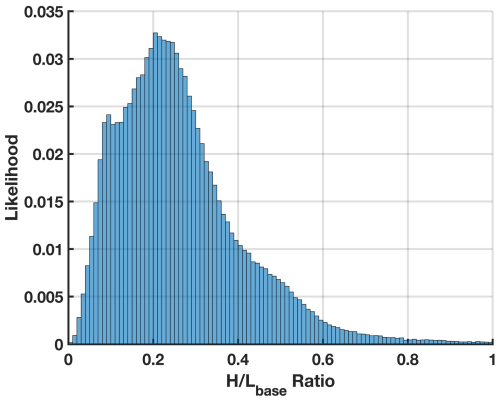
Figure 1 Distribution of $H/L_{\mathrm{base}}$ for coastal foredunes along the outer coast of the continental United States derived from Mull and Ruggiero (2014) and Doran et al. (2017), as compiled in Cohn (2022), where L_base is assumed to be the length scale from the dune toe to the dune crest.

In this work we aim to examine the limits and error trends of analytical bed shear stress predictions by comparing to computational fluid dynamics (CFD) simulations for a range of idealized dune profiles. Furthermore, we explore alternative data-driven models through symbolic regression (SR) methods and projection-based, non-intrusive, reduced-order modeling (NIROM) techniques. Our goal is to provide insight into the errors incurred by and subsequent sediment transport effects of using traditional theoretical bed shear stress predictions in dune evolution models, as well as to explore the advantages and disadvantages of some possible alternative flow modeling strategies. We begin by providing a brief overview of analytical bed shear stress predictions, the use of CFD in modeling flow dynamics over dunes, symbolic regression methods, and projection-based NIROM techniques in Sect. 2. In Sect. 3, we lay out our approach for using these methods to produce alternative bed shear stress predictions. Results of CFD, symbolic regression, and NIROM predictions and their comparison to KSH are examined in Sect. 4. Finally, an intercomparison of the methods considered and the subsequent impact on dune evolution models are discussed in Sect. 5.

2 Background

2.1 Analytical solutions for flow over low sloping dunes

One of the earliest analytical models for predicting the near-surface flow over a low-sloping hill was developed by Jackson and Hunt (1975). Given the overall height, H, and the characteristic length, L, defined as the half-length at half-height, the slope is assumed to be on the order of the height-to-length ratio, $H/L$, which is assumed to be small. Additionally, the characteristic length-to-roughness-length ratio, $L/z_{\mathrm{0}}$, which is assumed to be large and uniform, also plays a central role in the analysis. Jackson and Hunt (1975) split the atmospheric boundary layer into two regions where the outer layer is treated as inviscid, while flow in the inner layer is driven by the induced pressure gradient and turbulence effects. The various important dimensions and regions are depicted in Fig. 2. The Reynolds-averaged Navier–Stokes (RANS) equations are then linearized and a solution obtained through a series of scaling arguments and matched asymptotic expansions.

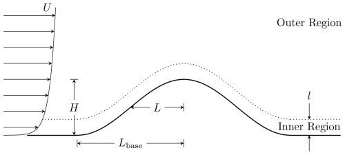
Figure 2 Sketch depicting the important geometric dimensions and regions for flow over simplified dune profiles.

Since the initial work of Jackson and Hunt (1975), the theory has been extended to three dimensions (Mason and Sykes, 1979), upstream velocity profiles with strong shear (Hunt et al., 1988), and higher-order corrections (Weng et al., 1991). However, the normalized bed shear stress perturbation remains essentially the same and is given by Weng et al. (1991) as

$$\begin{array}{}\text{(1)}& {\displaystyle }{\mathit{\tau }}^{\prime }={\displaystyle \frac{\mathit{\tau }}{{\mathit{\tau }}_{\mathrm{0}}}}-\mathrm{1}\text{(2)}& {\displaystyle }\mathcal{F}\left[{\mathit{\tau }}^{\prime }\right]={\displaystyle \frac{\mathrm{2}H/L}{U^{\mathrm{2}}\left(l\right)}}\mathcal{F}\left[{\mathit{\sigma }}^{\prime }\right][\mathrm{1}+{\displaystyle \frac{\mathrm{2}\ln \left|kL\right|+\mathrm{4}\mathit{\gamma }+\mathrm{1}+i\mathit{\pi }}{\ln (l/z_{\mathrm{0}})}}]\text{(3)}& {\displaystyle }{\mathit{\sigma }}^{\prime }={\displaystyle \frac{\mathrm{1}}{\mathit{\pi }}}\underset{-\mathrm{\infty }}{\overset{\mathrm{\infty }}{\int }}{\displaystyle \frac{f^{\prime }\left({\mathit{\xi }}^{\prime }\right)}{\mathit{\xi }-{\mathit{\xi }}^{\prime }}}\mathrm{d}{\mathit{\xi }}^{\prime },\end{array}$$

where σ^′ is the leading order normalized pressure perturbation given by the Hilbert transform of the hill slope, z₀ the surface roughness length, k the Fourier wave number, $\mathit{\xi }=x/L$ a normalized streamwise coordinate, γ≈0.57721 Euler's constant, and l the length scale of the inner region given by

$$\begin{array}{}\text{(4)}& l\ln \left({\displaystyle \frac{l}{z_{\mathrm{0}}}}\right)=\mathrm{2}{\mathit{\kappa }}^{\mathrm{2}}L.\end{array}$$

More recently, Kroy et al. (2002) further simplified the expression for a transverse dune, leading to

$$\begin{array}{}\text{(5a)}& {\displaystyle }\mathcal{F}\left[{\mathit{\tau }}^{\prime }\right]=A\left(\right|k|+iBk)\mathcal{F}\left[h\right(x\left)\right]\text{(5b)}& {\displaystyle }A={\displaystyle \frac{\ln ({\mathrm{\Phi }}^{\mathrm{2}}/\ln \mathrm{\Phi }{)}^{\mathrm{2}}}{\mathrm{2}(\ln \mathit{\varphi }{)}^{\mathrm{3}}}}[\mathrm{1}+\ln \mathit{\varphi }+\mathrm{2}\ln (\mathit{\pi }/\mathrm{2})+\mathrm{4}\mathit{\gamma }]\text{(5c)}& {\displaystyle }B=\mathit{\pi }[\mathrm{1}+\ln \mathit{\varphi }+\mathrm{2}\ln (\mathit{\pi }/\mathrm{2})+\mathrm{4}\mathit{\gamma }{]}^{-\mathrm{1}}\text{(5d)}& {\displaystyle }\mathit{\varphi }\equiv \mathrm{2}{\mathit{\kappa }}^{\mathrm{2}}\mathrm{\Phi }/\ln \mathit{\varphi }\text{(5e)}& {\displaystyle }\mathrm{\Phi }=L/z_{\mathrm{0}},\end{array}$$

where h(x) represents the dune topography and κ=0.41 is the von Kármán constant. It should be noted that we have retained the terms involving the logarithmic dependence on the characteristic length which stems from Eq. (2), i.e., $\mathrm{2}\ln (\mathit{\pi }/\mathrm{2})$, in contrast to the description in Kroy et al. (2002), which indicates that these terms are neglected in their subsequent analysis.

As alluded to earlier, three inherent limitations exist with these asymptotic-based analytical models when applying them to realistic coastal dunes. First, linearization of the underlying equations precludes the ability to capture separated flow effects. Traditionally, this has been overcome by extending the dune surface with an empirical separation bubble profile (Kroy et al., 2002; Schatz and Herrmann, 2006) or by applying a nonlinear correction to the predicted bed shear stress based on numerical simulations of forward- and backward-facing steps (Pelletier, 2009). However, it should be noted that these ad hoc extensions do not account for the dependence of the separating streamline and reattachment angle on the upwind shear velocity (Araújo et al., 2013). Additionally, by setting the shear stress to zero in these regions the potential for reverse transport in the lee is overlooked. Secondly, the assumption of a small $H/L$ and dune slope can lead to issues when applying the model to dunes with sharp local features, such as scarps, that may otherwise satisfy the $H/L$ criteria and not exhibit separation on the lee side. Again, while the shear stress perturbation can be limited to ${\mathit{\tau }}^{\prime }\ge -\mathrm{1}$ in the case of separation at a scarp (Durán Vinent and Moore, 2015), the presence of this locally steep topography influences the shear stress across the crest and in the lee of the dune as well (Bauer and Wakes, 2022), leading to additional errors. Additionally, the majority of dunes, at least in the coastal domain (e.g., Fig. 1), do not conform to the low-slope assumption, limiting the use of these analytical approaches to a small subset of morphological dune types. Finally, while the surface roughness, z₀, is assumed to be constant over the dune, realistic coastal dunes rarely exhibit a uniform surface roughness due to the inherent heterogeneity of vegetation growth. Nevertheless, these Fourier-transform-based physical approximations are simple to implement, provide rapid predictions, and have shown great utility in capturing a range of dune phenomena (Durán et al., 2010; Parteli and Herrmann, 2007), making them attractive for incorporation into larger dune evolution models (Walmsley and Howard, 1985; Stam, 1997; Kroy et al., 2002; Duran and Moore, 2013).

2.2 Computational fluid dynamics simulations of flow over dunes

While analytical predictions for the shear stress perturbation have played a major role in morphological studies, CFD approaches have also been important in understanding the flow dynamics over aeolian landforms (Smyth, 2016). One of the earliest is Wippermann and Gross (1986) in which the mesoscale meteorological model FITNAH, a nonhydrostatic, Reynolds-averaged Navier–Stokes (RANS) model, was used in lieu of a theoretical expression as discussed above to simulate the development and migration of a barchan, thus overcoming limitations of the linear predictions. Additionally, numerical simulations have been used to study the effects of varying height and length of an idealized transverse dune (Parsons et al., 2004a, b), varying roughness heights (Wakes et al., 2010), flow separation on the lee side of dunes (Schatz and Herrmann, 2006; Araújo et al., 2013), and airflow over scarps (Hesp and Smyth, 2021; Bauer and Wakes, 2022), as well as blowouts (Smyth et al., 2012), reversing dunes (Jackson et al., 2020), and nebkha foredunes (Hesp and Smyth, 2017; Furtak-Cole et al., 2022). Other example works include Jackson et al. (2011), which compared several turbulence models including RANS k−ω SST, several hybrid RANS–LES models without surface roughness effects, and an LES–ABL model that included the surface roughness, highlighting the importance of capturing surface roughness effects, as well as Jackson et al. (2013), which presented full 3D RANS simulations for a large dune field. Of particular relevance to the current study, Ferreira et al. (2013) showed that CFD predictions achieve generally good agreement with experimental measurements of shear stress distributions for single and tandem dunes. In general, (OpenFOAM Ltd., 2020) has become a widely used CFD tool for modeling wind dynamics and bed shear stress over topography, including in coastal environments (e.g., Hesp et al., 2015; Jackson et al., 2013).

2.3 Symbolic regression

Existing analytical solutions for the effective bed shear stress distribution over dunes are relatively fast and easy to implement but lack the accuracy and general validity of full CFD simulations. One possible way to bridge this gap is through data-driven techniques. For example, Wakes et al. (2021) trained machine learning models, including random forest and logistic regression approaches, on CFD model output to generate flow predictors. However, there are a number of methods which have yet to be explored or fully evaluated. In particular, symbolic regression (SR) is a long-standing approach that has seen recent growth due to the emergence of new machine learning tools and techniques (Koza, 1994; Champion et al., 2020; Bakarji et al., 2023; Makke and Chawla, 2024). As its name suggests, SR seeks to identify a symbolic expression using a combination of provided input features, symbolic operators, and constants which best captures the relationship between input and output. While SR may lack the accuracy and training efficiency for large, multi-dimensional datasets achieved by deep neural networks, the resulting analytical expressions are more interpretable and often more generalizable than their neural network counterparts.

Some of the most popular methods for discovering the optimal input–output mapping are the Sparse Identification of Nonlinear Dynamics (SINDy) (Brunton et al., 2016), genetic programming-based approaches (Koza, 1994), and more recent efforts to incorporate neural network and deep learning techniques (Sahoo et al., 2018; Petersen et al., 2019). In SINDy and its variants (Rudy et al., 2019; Champion et al., 2019, 2020; Kaheman et al., 2020; Shea et al., 2021; Fasel et al., 2022), a precomputed library of nonlinear terms along with sparse optimization techniques such as the least absolute shrinkage and selection operator (LASSO) (Brunton et al., 2016) or sequential threshold ridge regression (STRidge) (Rudy et al., 2017) are used to determine a sparse, optimal, linear combination of nonlinear terms. While the SINDy approach is computationally efficient, it is known to struggle with noisy data and is limited in the functional forms that it is able to learn (Makke and Chawla, 2024).

On the other hand, genetic programming (GP) approaches utilize data structures, such as expression trees (Koza, 1994) or imperative representations (Brameier and Banzhaf, 2007) that allow for more general functional forms. However, the use of evolutionary strategies to search the space formed by the combination of input features, operators, and possibly real constants incurs a greater computational cost. In general, GP approaches begin with a randomly seeded initial population of candidate expressions that is then evolved over several generational cycles. Each cycle consists of evaluating the existing candidates, selecting candidates for mutation, and finally mutating expressions to create a new set of candidates (Koza, 1994). The fitness of all candidates is tracked over the course of many iterations and the best overall candidate is selected as the solution.

One recent GP-based SR tool is PySR (Cranmer, 2023). In addition to the basic GP formulation, it includes regularized evolution for updating population members, a simplify–optimize stage that aims to reduce the number of equivalent but symbolically different expressions and reduce the burden of discovering equations with floating point constants, and a parsimony penalty which aims to maintain equal numbers of candidate expressions at every level of complexity (Cranmer, 2023). In this paper, we apply PySR to CFD simulation data (Cecil et al., 2024) and evaluate its performance compared to the classical KSH functional and a class of reduced-order modeling techniques that we describe next.

2.4 Non-intrusive reduced-order modeling

Another possible way to bridge the gap between classical analytical techniques and full CFD simulations is to build a surrogate (or reduced-order) version of the CFD model itself. If successful, this approach can combine the physical fidelity of a RANS or LES approximation with the speed of a closed-form analytical expression. A vast and growing body of literature exists on reduced-order modeling (e.g., Hesthaven et al., 2016; Benner et al., 2015; Lee and Carlberg, 2020; Brunton et al., 2020). The fundamental idea underlying these approaches is that high-fidelity simulation data often exhibit dynamics with low-dimensional structure. One of the most popular ways to exploit this structure is through the method of snapshots and projection-based model reduction (Carlberg et al., 2017; Benner et al., 2015). In this case, one first generates a set of high-fidelity simulation data (or snapshots) and identifies a low-dimensional approximation to the solution subspace (or manifold) through a dimension reduction step. Reduced-order solutions are then expressed as an expansion in a basis that spans the solution subspace (Dutta et al., 2021a). Traditional techniques like proper orthogonal decomposition (POD) use linear dimension reduction, while nonlinear techniques based on deep neural network architectures are becoming increasingly popular for problems with complex, multi-scale dynamics (Wan et al., 2018; Lee and Carlberg, 2020; Maulik et al., 2021; Dutta et al., 2022).

If the governing equations are known and accessible through the high-fidelity model, one can use Galerkin or Petrov–Galerkin projection to create a rigorous, interpretable reduced-order model (ROM) (Carlberg et al., 2013; Lozovskiy et al., 2016, 2017). Often, this is not practical (or possible) due to design of the high-fidelity model or restrictions on access to its source code. For these cases, purely data-driven methods that do not require intrusive access to the high-fidelity model have become popular (Xiao et al., 2017; Dutta et al., 2021b). Rather than using Galerkin or Petrov–Galerkin projection, these non-intrusive ROMS (NIROMs) use black-box interpolation (or regression) to obtain expansion coefficients for the approximate solution in the reduced basis. A wide array of interpolation techniques and strategies have been tested including Gaussian process regression (Guo and Hesthaven, 2019), dynamic mode decomposition (Tu et al., 2014; Wu et al., 2021), radial basis functions (RBFs) (Walton et al., 2013; Xiao et al., 2015; Dutta et al., 2021a), and neural networks (Hesthaven and Ubbiali, 2018; Salvador et al., 2021; Dutta et al., 2021c). In each case, data for the NIROM interpolation are provided by the projection coefficients of the original simulation snapshots. As a result, the success of the resulting ROM depends heavily on balancing accuracy with over-fitting and having training data that adequately represent the problem space of interest (Dutta et al., 2021a).

Below, we will employ well-established NIROM techniques based on linear dimension reduction and RBF interpolation to build reduced-order approximations of high-fidelity CFD simulations over various dune profiles. These results will serve as benchmarks to evaluate the accuracy and generalizability of our SR approximations.

3 Methodology

3.1 Prescribed dune shapes for modeling

In real-world systems, dunes take on a wide range of shapes and sizes (e.g., Fig. 1). To examine the influence of variable topography on bed shear stress patterns, for this study we examined four types of dune profiles that have been parameterized to allow for consistent specification of the height H and characteristic length L given by the half-length at half-height. These include a quadratic cosine, Gaussian, quartic, and bump profile given by the following.

$$\begin{array}{}\text{(6a)}& {\displaystyle }\begin{array}{rl}& \text{Cosine:}h\left(x\right)=a_{\mathrm{c}}{\cos }^{\mathrm{2}}\left[b_{\mathrm{c}}\right(x-\mathit{\sigma }\left)\right];a_{\mathrm{c}}=H;\\ & b_{\mathrm{c}}={\displaystyle \frac{\mathrm{1}}{L}}\arccos \left(\sqrt{\frac{\mathrm{1}}{\mathrm{2}}}\right);x\in [-{\displaystyle \frac{\mathit{\pi }}{\mathrm{2}{b}_{\mathrm{c}}}}+\mathit{\sigma },{\displaystyle \frac{\mathit{\pi }}{\mathrm{2}{b}_{\mathrm{c}}}}+\mathit{\sigma }]\end{array}\text{(6b)}& {\displaystyle }\begin{array}{rl}& \text{Gaussian:}h\left(x\right)=a_{\mathrm{g}}\exp \left[-{\displaystyle \frac{(x-\mathit{\sigma }{)}^{\mathrm{2}}}{b_{\mathrm{g}}}}\right];a_{\mathrm{g}}=H;\\ & b_{\mathrm{g}}=-L^{\mathrm{2}}{\ln }^{-\mathrm{1}}\left(\frac{\mathrm{1}}{\mathrm{2}}\right)\end{array}\text{(6c)}& {\displaystyle }\begin{array}{rl}& \text{Quartic:}h\left(x\right)={\displaystyle \frac{a_{\mathrm{q}}}{\mathrm{1}+b_{\mathrm{q}}(x-\mathit{\sigma }{)}^{\mathrm{4}}}};a_{\mathrm{q}}=H;\\ & b_{\mathrm{q}}={\displaystyle \frac{\mathrm{1}}{L^{\mathrm{4}}}}\end{array}\text{(6d)}& {\displaystyle }\begin{array}{rl}& \text{Bump:}h\left(x\right)=a_{\mathrm{b}}\exp \left[{\displaystyle \frac{-\mathrm{1}}{\mathrm{1}-b_{\mathrm{b}}(x-\mathit{\sigma }{)}^{\mathrm{2}}}}\right];a_{\mathrm{b}}=He;\\ & b_{\mathrm{b}}={\displaystyle \frac{\mathrm{1}+[\mathrm{1}/\ln (\frac{\mathrm{1}}{\mathrm{2}}\left)\right]}{L^{\mathrm{2}}}};x\in [\sqrt{\frac{\mathrm{1}}{b_{\mathrm{b}}}}+\mathit{\sigma },-\sqrt{\frac{\mathrm{1}}{b_{\mathrm{b}}}}+\mathit{\sigma }]\end{array}\end{array}$$

Here, σ specifies the x location of the dune peak and h represents the local bed elevation. When applying symbolic regression in Sect. 3.2.3, the shift, σ, becomes important for recovering both real and imaginary parts of the Fourier-transformed expression in Eq. (5).

The profile elevations and slopes are plotted in Fig. 3 for $H/L=\mathrm{0.1}$. It should be noted that while all of the profiles can be controlled to have a small height-to-length ratio as shown in Fig. 3a, only the Gaussian and quartic profiles fulfill the small slope requirement (i.e., $h^{\prime }\left(x\right)=\mathcal{O}(H/L)$) as depicted in Fig. 3b. The cosine profile represents a moderate departure from this constraint and the bump profile a more extreme case that is representative of a scarp. Thus, these profiles allow us to explore not only the effect of increasing $H/L$ ratios on the accuracy of the KSH model, but also the limitations of the underlying small slope assumption when it is not implicitly imposed by a small height-to-length ratio.

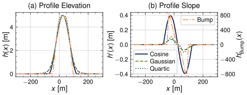
Figure 3 Comparison of prototype dune profile (a) and slopes (b). Note that the bump profile slope uses the right y axis in panel (b) due to the large difference in scale between it and the other profiles.

For all cases considered, the length-to-aerodynamic-roughness ratio, $L/z_{\mathrm{0}}$, is held constant at $\mathrm{\Phi }=L/z_{\mathrm{0}}=\mathrm{25000}$ by choosing L=25 m and $z_{\mathrm{0}}=\mathrm{1}\times {\mathrm{10}}^{-\mathrm{3}}\text{m}$, leading to the KSH model coefficients A=5.1952 and B=0.2793 (AB=1.4510) that remain constant across all cases. Three sets of $H/L$ ratios are considered, namely a small set with $H/L\in [\mathrm{0.01},\mathrm{0.1}]$, medium with $H/L\in [\mathrm{0.1},\mathrm{0.3}]$, and large with $H/L\in [\mathrm{0.3},\mathrm{0.5}]$. In reference back to Fig. 1, the bump profile has L_base=37.57 m, leading to a maximum $H/L_{\mathrm{base}}$ of 0.3, and for the cosine profile L_base=50 m, yielding a maximum $H/L_{\mathrm{base}}$ of 0.25. This captures ∼ 35 % of the coastal foredune aspect ratios presented in Fig. 1 assuming L_base≈2.5 L to account for the quartic and Gaussian profiles. A summary of the case properties is given in Table 1.

Table 1 Details of base case sets.

3.2 Modeling of shear stress perturbations

3.2.1 CFD simulations

Computational fluid dynamic simulations were run for the medium and large case sets described in the previous section using the open-source solver OpenFOAM. Specifically, the Reynolds-averaged Navier–Stokes (RANS) equations were solved with the RNG k−ϵ turbulence model using the incompressible SimpleFOAM solver. Second-order accurate discretization schemes were used throughout. More precisely, the least-squares method was applied for determining cell-centered gradient values with a cubic limiter for the velocity components and turbulence quantities. The linear upwind scheme was chosen for divergence terms and the linear scheme for Laplacian terms. At the inlet, an atmospheric boundary layer (ABL) profile (Richards and Hoxey, 1993; Yang et al., 2009) was specified according to

$$\begin{array}{}\text{(7)}& {\displaystyle }u={\displaystyle \frac{u^{*}}{\mathit{\kappa }}}\ln \left({\displaystyle \frac{z-d+z_{\mathrm{0}}}{z_{\mathrm{0}}}}\right)\text{(8)}& {\displaystyle }v=w=\mathrm{0}\text{(9)}& {\displaystyle }k={\displaystyle \frac{(u^{*}{)}^{\mathrm{2}}}{\sqrt{C_{\mathit{\mu }}}}}\text{(10)}& {\displaystyle }\mathit{ϵ}={\displaystyle \frac{(u^{*}{)}^{\mathrm{3}}}{\mathit{\kappa }(z-d+z_{\mathrm{0}})}}\text{(11)}& {\displaystyle }{u}^{*}={\displaystyle \frac{u_{\text{ref}}\mathit{\kappa }}{\ln \left(\frac{z_{\text{ref}}+z_{\mathrm{0}}}{z_{\mathrm{0}}}\right)}},\end{array}$$

where $u^{*}=\sqrt{\mathit{\tau }/\mathit{\rho }}$ is the friction velocity, C_μ=0.09 is a model constant, k the turbulent kinetic energy, and ϵ is the turbulent kinetic energy dissipation rate. In order to maintain the inlet profile over the approach stretch, a constant shear stress condition was applied to the velocity at the top boundary (Richards and Hoxey, 1993; Hargreaves and Wright, 2007; Richards and Norris, 2019). At the surface, a wall function specific to ABL simulations (Richards and Hoxey, 1993; Parente et al., 2011) as implemented in OpenFOAM's atmEpsilonWallFunction was used, and the turbulent viscosity was constrained by the atmNutkWallFunction. A reference velocity of $u_{\text{ref}}=\mathrm{10}{\text{m\hspace{0.17em}s}}^{-\mathrm{1}}$ at a reference height of z_ref=10 m was used for all cases.

The computational domain consisted of a rectangular area that was 425 m long with a total height 200 m greater than the height of the dune crest H. The dunes were positioned such that their crest is located at x=30 m, while the computational domain was symmetric about x=0 m, resulting in the crest being 242.5 m downwind of the inlet and 182.5 m from the outflow boundary. A uniform base discretization of 1 m was created using blockMesh and subsequently refined near the surface to between 0.0625 and 0.125 m using SnappyHexMesh. Additionally, approximately 20 anisotropic surface layers were inserted with the first cell height adjusted per case to maintain y⁺ values between approximately 30 and 200. This corresponds to a minimum first cell height of $\mathrm{5.138}\times {\mathrm{10}}^{-\mathrm{3}}\text{m}$ obtained for the quartic profile with $H/L=\mathrm{0.5}$. Simulations were run to steady state with convergence established when all residuals had fallen to at least $\mathrm{1}\times {\mathrm{10}}^{-\mathrm{8}}$ and the iteration-to-iteration change of the calculated drag over the hill profile was less than $\mathrm{1}\times {\mathrm{10}}^{-\mathrm{8}}$.

3.2.2 CFD data preparation

The geometry representations and shear stress results of the CFD simulations provide a dataset to which data-driven model discovery tools can be applied. To begin, the surface topography and total shear stress were extracted using OpenFOAM's sampling utilities. Even spacing between samples for subsequent Fourier transforms was ensured by resampling the data at an equivalent number of points using cubic spline interpolation. Furthermore, some of the leading and trailing ends of the domain (i.e., 150 points, ∼ 9 m, at either end of the 6800 total samples, ∼ 425 m) were truncated to avoid spurious boundary affects. The bed shear stress perturbation was then recovered using Eq. (1) where the value at the leading edge of the truncated domain was used for normalization. Furthermore, the results were filtered to remove high-frequency noise in both the topography and shear stress and downsampled to N=650 samples to obtain a reasonably sized, high-fidelity dataset for performing SR and reduced-order modeling.

3.2.3 Symbolic regression

Using the processed CFD data, discrete Fourier transforms (DFTs) were taken of the topography and shear stress perturbation. These along with the Fourier wave numbers were provided to PySR to solve the minimization problem,

$$\begin{array}{}\text{(12)}& \underset{f\left(\right)}{min}{\left|\left|\mathcal{F}\left[{\mathit{\tau }}^{\prime }\right]-f\left(\mathcal{F}\right[h\left(x\right)],k)\right|\right|}_{\mathrm{2}},\end{array}$$

in complex Fourier space where f() denotes an unknown function residing in the space of operators consisting of addition, subtraction, multiplication, and absolute value as well as additional complex constants. PySR's regularized evolution algorithm was run for 100 iterations where each iteration consists of multiple rounds of tournament selection and mutation (Cranmer, 2023). Several of the default hyperparameters were adjusted in order to obtain consistent results across all cases for several different levels of synthetic noise (see Sect. 4.2.1). A listing of non-default options that were supplied to PySR is available in Table A1 located in Appendix A. Finally, after obtaining the optimal expression f(⋅) from PySR, the bed shear stress perturbation in real space is given by

$$\begin{array}{}\text{(13)}& {\mathit{\tau }}^{\prime }={\mathcal{F}}^{-\mathrm{1}}\left[f\right(\mathcal{F}\left[h\right(x\left)\right],k\left)\right],\end{array}$$

where ${\mathcal{F}}^{-\mathrm{1}}[\cdot ]$ indicates the inverse Fourier transform.

3.2.4 Non-intrusive reduced-order modeling

In addition to the CFD and symbolic regression approaches, we also explore predictions based on linear NIROM techniques. As discussed earlier, this basic approach relies on selecting a low-dimensional, data-driven basis for the approximate solution that ideally captures essential solution behavior at much reduced computational cost. That is, we write the approximate solution $\stackrel{\mathrm{̃}}{\mathit{y}}$ in ℝ^N on the downsampled CFD grid as

$$\begin{array}{}\text{(14)}& \stackrel{\mathrm{̃}}{\mathit{y}}=\sum _{j=\mathrm{1}}^m{z}_j{\mathit{u}}_j,\end{array}$$

where $\mathit{\{}{\mathit{u}}_j{\mathit{\}}}_{j=\mathrm{1}}^m,$ u_j∈ℝ^N is the basis and ideally m≪N. Next, a regression model is constructed to capture the parameterized relationship between the input topography and output surface shear stress perturbation. To do this, we represent the topography, h∈ℝ^N, on the downsampled CFD grid as

$$\begin{array}{}\text{(15)}& \mathit{h}=\sum _{j=\mathrm{1}}^m{c}_j{\mathit{d}}_j,\end{array}$$

where $\mathit{\{}{\mathit{d}}_j{\mathit{\}}}_{j=\mathrm{1}}^m,$ d_j∈ℝ^N is a low-dimensional basis for the topography space. A regression metamodel $G:\mathit{c}\to \mathit{z}$ then maps the discrete input to output coefficients {z_j}, and the approximate solution is given by Eq. (14).

For an alternative basis, we explore either a truncated Fourier basis in which the original theoretical model resides or a POD expansion (Rathinam and Petzold, 2003). There are pros and cons to each reduced space approximation. POD provides an optimal representation of the training (snapshot) data in terms of the Euclidean 2-norm (Quarteroni et al., 2016) and hence better data compression, while a Fourier basis requires more modes for smooth reconstruction (≈80 modes for the simulations considered below) but provides better generalization to unseen data.

Below, for the POD basis we combine both the input topography profiles and resulting CFD-based shear stress perturbations into a composite dataset and generate a single basis for both. That is, we perform n_s training simulations and compute a singular value decomposition:

$$\begin{array}{}\text{(16)}& \mathbf{S}=\mathbf{U}\mathbf{\Sigma }{\mathbf{W}}^T,\end{array}$$

where the columns of the snapshot matrix $\mathbf{S}\in {\mathbb{R}}^{N\times \mathrm{2}{n}_{\mathrm{s}}}$ hold both the input topographies $\mathit{\{}{\mathit{d}}_j{\mathit{\}}}_{j=\mathrm{1}}^{n_{\mathrm{s}}}$ and shear stress perturbations $\mathit{\{}{\mathit{y}}_j{\mathit{\}}}_{j=\mathrm{1}}^{n_{\mathrm{s}}}$. The first m columns of U, $\mathit{\{}{\mathit{u}}_j{\mathit{\}}}_{j=\mathrm{1}}^m$ form the solution and topography basis (i.e., ${\mathit{d}}_j={\mathit{u}}_j\forall j=\mathrm{1},\mathrm{\dots },m$). Then for a given topography input evaluated on the CFD grid, h, we compute the projection c=D^Th, where $\mathbf{D}\in {\mathbb{R}}^{N\times m}$ is a matrix holding the basis elements {d_j} as columns and similarly for the shear stress perturbation to obtain z.

For the Fourier basis, d_j and u_j are obtained through DFTs, which are truncated by zeroing elements beyond the selected number of modes. Subsequently, the complex Fourier representations are split into real and imaginary parts and individual metamodels constructed for $\mathcal{R}\left(G\right):\mathcal{R}\left(\mathit{c}\right)\to \mathcal{R}\left(\mathit{z}\right)$ and $\mathcal{I}\left(G\right):\mathcal{I}\left(\mathit{c}\right)\to \mathcal{I}\left(\mathit{z}\right)$. The final predictions are then generated via

$$\begin{array}{}\text{(17)}& \stackrel{\mathrm{̃}}{\mathit{y}}={\mathcal{F}}^{-\mathrm{1}}\left[\mathcal{R}\right(G)+\mathcal{I}(G\left)\right].\end{array}$$

For constructing the regression metamodels in the latent space we use RBF interpolation to capture the input–output mapping with either a Gaussian kernel using a shape parameter of 0.1 and additional linear polynomial (for the POD basis) or a multi-quadric kernel using a shape parameter equal to 0.1 and a zero-degree polynomial (for the Fourier basis). While we proceed here by choosing either a random set across all four profiles or all cases of two profiles to construct the POD basis and train the metamodel, there are alternative selection criteria that could be considered such as the standard and greedy approaches found in Dutta et al. (2021a). Furthermore, there is still significant flexibility within the above framework for how the input parameter space is sampled to generate snapshots and how these are used to generate the reduced bases and regression mappings. For example, a separate POD basis could be constructed for the input and output or regression performed in complex space for the Fourier-based approach.

3.3 Model skill metrics

To assess differences between the various models, we examine the mean square error (MSE) defined by

$$\begin{array}{}\text{(18)}& \text{MSE}=(\mathrm{1}/N)\sum _{i=\mathrm{0}}^N(y_i-{\stackrel{\mathrm{̃}}{y}}_i{)}^{\mathrm{2}},\end{array}$$

where the CFD results are taken as the target values, y_i, and the KSH, SR, or NIROM results as the predictions, ${\stackrel{\mathrm{̃}}{y}}_i$, as well as the maximum error across all spatial locations. In the results presented below all errors are calculated for the shear stress perturbations and are therefore analogous to a relative error for the total bed shear stress.

4 Results

4.1 CFD predictions

We begin by examining the results of the CFD simulations compared to the theoretical predictions of Eq. (5) in Fig. 4. Representative results for the surface shear stress distribution are provided for the bump and Gaussian profiles for two $H/L$ ratios in Fig. 4a–d. Our CFD simulations predict separation in the lee for $H/L\ge \mathrm{0.3}$ for the bump profile, $H/L\ge \mathrm{0.38}$ for the quartic, and $H/L\ge \mathrm{0.5}$ for the cosine, while the flow remains attached for all of the Gaussian cases considered.

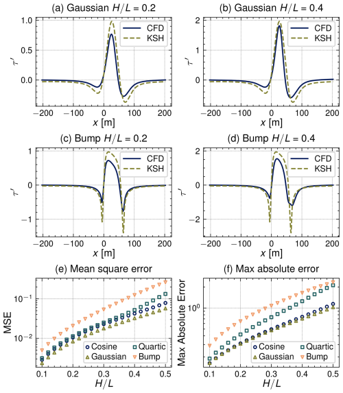
Figure 4 Comparison of CFD simulation results and KSH predictions. Bed shear stress perturbation predictions for selected cases are presented in panels (a–d). The mean square error for each case is given panel (e) and the maximum absolute error in panel (f).

In what follows, it should be noted that we have compared our CFD results to unmodified predictions from the other models. In practice, the shear stress perturbation prediction from KSH is usually limited to values greater than or equal to −1 in recognition of validity constraints imposed by the underlying assumptions. On the lee side, separation streamlines are typically defined using phenomenological fits of either a cubic polynomial (Kroy et al., 2002) or ellipse (Schatz and Herrmann, 2006) based on the dune geometry to improve prediction on the stoss slope. However, these approaches prove difficult to implement when a clear brink or separation location cannot be identified, as in the case of the current profiles, and fail to account for additional factors controlling the extent of the separating streamline such as the upwind shear velocity (Walker and Nickling, 2002; Araújo et al., 2013). For these reasons, and in an effort to produce a consistent comparison among all models, we have used the unmodified predictions of τ^′ over the actual idealized profiles.

The MSE and maximum error are plotted for each of the four profiles and 21 $H/L$ ratios in Fig. 4e and f. Here we can clearly see that the error increases with increasing $H/L$ as is to be expected from the assumptions present in the KSH model. Additionally, the errors for the bump profile, which drastically violates the low-slope assumption while satisfying a small $H/L$, are greater than the other profiles for each value of $H/L$. In fact, referring back to Fig. 3b, the MSE increases for increasing max slope except for the quartic case, which is roughly equivalent to the cosine profile until $H/L\approx \mathrm{0.4}$, at which point the MSE for the quartic profile begins to increase at a faster rate.

Next, we examine the spatial distribution of absolute error in Fig. 5. Interestingly, the error in maximum shear stress prediction (just ahead of the dune crests situated at x=30 m) from the KSH model either stays relatively constant or decreases for increasing $H/L$. The most drastic increase in prediction error comes on the lee side of the dune profiles where separation is most likely to occur. Again, considering the slope of the different profiles, the bump profile exhibits two distinct regions of higher error just fore and aft of the main dune body where the slopes are highest. This effect is drastically reduced in the other profiles which exhibit much gentler slope characteristics.

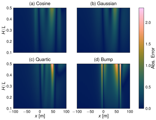
Figure 5 Spatial distribution of absolute difference between OpenFOAM and KSH bed shear stress perturbation predictions. Note that the x domain has been limited to highlight the area of interest immediately surrounding the dune.

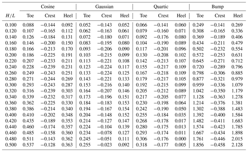
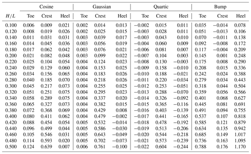
Finally, the differences in the surface shear stress perturbation extrema predicted by CFD and KSH are tabulated in Table 2. The difference in the local minima near the dune toe consistently increases with increasing $H/L$. However, the differences in maxima near the crest and local minima near the heel exhibit more nuanced behavior depending on the profile. For example, the cosine, Gaussian, and quartic profile difference magnitudes in maximum τ^′ increase until $H/L\approx \mathrm{0.26}$ before decreasing as $H/L$ continues to increase. However, for the bump profile, the absolute value of the difference in maximum τ^′ increases consistently for the range of $H/L$ considered. A similar observation can be made for the minima in the lee, except for the cosine profile, which exhibits a consistent increase in difference as well. Considering this in light of Figs. 5 and 4e, which show a consistent increase in absolute error and MSE, respectively, suggests that the overall errors are due not only to differences in magnitude but also differences in the phase prediction with respect to the topography and overall distribution of τ^′.

Table 2 Differences in surface shear stress extrema predictions between CFD and KSH. Values are reported for local minima near the dune toe and heel, as well as the maximum near the dune crest for each profile and $H/L$ considered.

4.2 Symbolic regression predictions

4.2.1 Symbolic regression on KSH

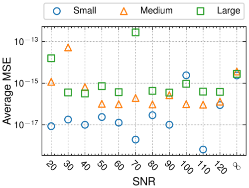
To begin exploring the use of symbolic regression via PySR, we first applied the methodology to data directly generated by the KSH model. After generating shear stress perturbation predictions for each of the hill profiles and height-to-length ratios using Eq. (5), we applied Gaussian noise at several signal-to-noise ratios (SNRs) to the shear stress perturbations. This was done in order to evaluate PySR's robustness to noise in measured output data in anticipation of dealing with the potentially noisy CFD predictions. PySR was trained on each of the small, medium, and large case sets using 8 cases for training and the remaining 36 cases for validation.

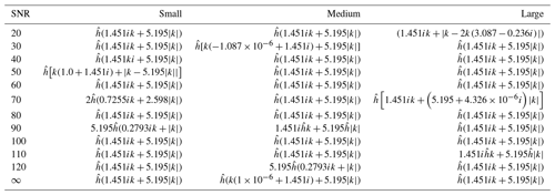
The average MSEs for each of the sets and SNRs considered are depicted in Fig. 6. In nearly all cases, PySR was able to learn the KSH model form and coefficient values. For those cases in which agreement of the symbolic form was not exact, e.g., the large set with SNR=20, the resulting expression still exhibited very low error. A table of each of the discovered expressions is supplied in Appendix A. Having determined that the PySR symbolic regression package was capable of discovering the underlying expression for analytically generated data in the Fourier domain and was robust to noise in the output variable, we turned our attention to applying SR to the CFD-generated data.

Figure 6 Average MSE across all profiles for each set of $H/L$ ratios in Table 1 and several SNRs.

4.2.2 Symbolic regression on CFD

Having shown that PySR is capable of discovering the KSH model from directly generated data, we next applied PySR to the processed CFD results for the medium set of $H/L$ values for which the flow remains attached for all cases. For this set, PySR returned a symbolic expression that nearly matches the form of the KSH model, differing only in the value of the multiplicative constants with AB picking up a negligible real part given by

$$\begin{array}{}\text{(19)}& \mathcal{F}\left[{\mathit{\tau }}^{\prime }\right]=\left(\mathrm{3.29}\right|k|+(\mathrm{1.62}i-\mathrm{1.8}\times {\mathrm{10}}^{-\mathrm{6}}\left)k\right)\mathcal{F}\left[h\right].\end{array}$$

It should be noted that physics-based constraints were not explicitly enforced in the SR training that led to Eq. (19). However, physics considerations are implicitly included since the training data were provided by physics-based CFD models and we have performed the regression on the Fourier transform of the input–output features in following with the asymptotic solutions. We believe this emphasizes the applicability of the linearized, asymptotic predictions to cases where separation is not present as well as the potential for SR to discover generalized expressions from data reflecting the underlying physics in some scenarios.

Being of the same form as KSH, Eq. (19) essentially represents an optimization of the model coefficients. The discovered value for A=3.29 is significantly lower than suggested by KSH, while B=0.492 is greater. It is known that the asymptotic expressions in Eq. (5) overpredict the value of A while underpredicting the value of AB (Charru et al., 2013). The results presented in Charru et al. (2013) obtained using a full numerical solution to the turbulent boundary layer predict A between 3 and 4 depending on the closure model, while AB is less than 2, which is in agreement with our result of A=3.29 and AB=1.62. It should also be noted that the error between the full solution and asymptotic predictions for A decreases as $L/z_{\mathrm{0}}$ increases, while the error for AB remains relatively constant (Charru et al., 2013). This suggests that our CFD results, and thus SR predictions for A and B, would be closer to the KSH predictions for higher values of $L/z_{\mathrm{0}}$.

Results using Eq. (19) are summarized in Fig. 7. As can be seen in Fig. 7a–d, the PySR model tends to underpredict the maximum shear stress perturbation in contrast to the standard KSH predictions while still overpredicting the minima just fore and aft of the dune. However, overall the PySR discovered model results in roughly an order of magnitude improvement in MSE for $H/L$ values between 0.1 and 0.3 as shown in Fig. 7e. However, results are more muted when extending this model to the larger $H/L$ values for which separation may occur. This can largely be attributed to the limitations of the linearized KSH model, and thus the SR learned model with an identical functional form, to be able to capture separation effects without ad hoc corrections. Additionally, when considering the spatial distribution of absolute error in Fig. 8, the error near the dune crest increases with successively higher values of $H/L$, in contrast to results for KSH in Fig. 5. Also, the shape of the shear stress perturbation near the peak of the bump profile is better captured, while the largest error still occurs just fore and aft where the slopes are steepest.

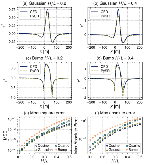
Figure 7 Comparison of CFD and symbolic regression predictions on the medium case set, i.e., Eq. (19). Selected bed shear stress perturbation profiles are shown in panels (a–d) with the MSE and max absolute error in panels (e) and (f), respectively.

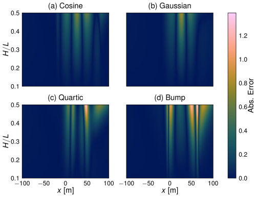
Figure 8 Spatial absolute difference between CFD and symbolic regression trained on select cases from the medium case set, i.e., Eq. (19).

Differences in the τ^′ extrema predictions between CFD and Eq. (19) are tabulated in Table 3. The differences in local minima near the dune toe are consistently improved over their KSH counterparts. However, the differences in maximum τ^′ are only improved for low $H/L$ and exhibit a monotonic increase for increasing $H/L$, showing degraded predictions compared to KSH for $H/L$ greater than approximately 0.28, except for the bump profile which exhibits consistent improvement over KSH. In the lee, results are again more nuanced depending on the profile considered. Improvement over KSH is seen for the cosine, Gaussian, and bump profiles, while the results for the quartic are somewhat degraded. Again, considering these results along with Fig. 8, it appears that Eq. (19) captures the phase advance and overall distribution of τ^′ more accurately (particularly for the cosine, Gaussian, and bump profiles) than KSH for the cases considered, and hence the overall MSE can largely be attributed to differences in magnitude.

Table 3 Differences in surface shear stress extrema predictions between CFD and Eq. (19). Values are reported for local minima near the dune toe and heel, as well as the maximum near the dune crest for each profile and $H/L$ considered.

In an effort to obtain better generalizability to separated cases, we next applied PySR to the large case set with somewhat unsatisfying results. Several trials were run using PySR while varying the number of cases provided, the cases selected for training, i.e., separated only or separated and attached scenarios, and the operator space to search. The most promising result obtained takes the form of the KSH model with several additional terms that are quadratic in the wave number given by

$$\begin{array}{}\text{(20)}& \begin{array}{rl}\mathcal{F}\left[{\mathit{\tau }}^{\prime }\right]& =(-\mathrm{2.32}\mathcal{F}[h\left]\right|k|+\mathcal{F}[h\left]\right)\left[\right(\mathrm{3.26}\times {\mathrm{10}}^{-\mathrm{6}}\\ & +i\mathrm{2.20})k+\mathrm{4.84}|k|-\mathrm{0.0380}+i\mathrm{1.81}\times {\mathrm{10}}^{-\mathrm{7}}].\end{array}\end{array}$$

Note that Eq. (20) contains terms representing the second derivative of the dune profile, thus increasing the model sensitivity to the underlying topography representation. Results obtained using Eq. (20) are summarized in Fig. 9. The trends in Fig. 9a–d are similar to the previous results; however, for the bump profile, while the minimums appear to be predicted better, some oscillatory behavior also appears in the results. This could be attributed to the inclusion of second derivative terms and the large spikes in the second derivative of the bump profile in those areas. Concerning the max error in Fig. 9f, the bump and cosine profiles exhibit a slower increase in maximum error until $H/L\approx \mathrm{0.35}$. The spatial distribution of error in Fig. 10 also exhibits trends similar to the previous results.

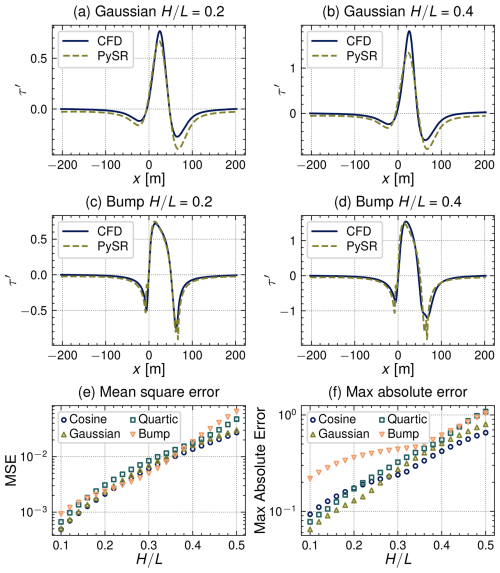
Figure 9 Comparison of CFD and symbolic regression predictions trained on the large case set, i.e., Eq. (20). Selected bed shear stress perturbation profiles are provided in panels (a–d) with the MSE and max absolute error for all cases in panels (e) and (f), respectively.

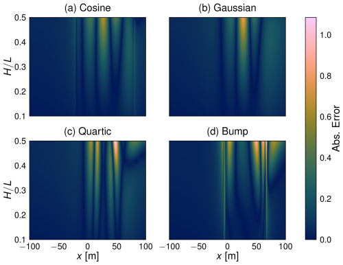
Figure 10 Spatial absolute difference between CFD and symbolic regression trained on cases from the large case set, i.e., Eq. (20).

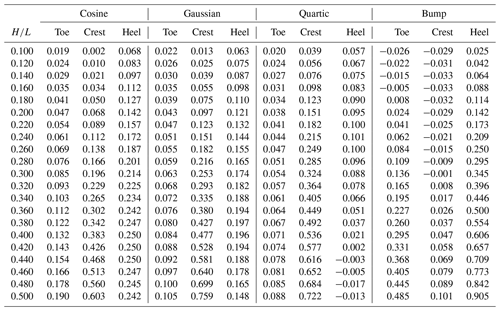
The differences in τ^′ extrema predictions between CFD and Eq. (20) are tabulated in Table 4. Results are generally comparable to the results obtained using Eq. (19) in Table 3, especially for the local minima near the toe and the maximum near the crest. For the minima in the lee, results are more profile-dependent, with a decrease in accuracy seen for the cosine and Gaussian cases, but improvements are gained for the quartic and bump profiles. Overall, Eq. (20) provides some modest improvement for errors over the bump profile, while little is gained for the other profiles considered. This could be attributed to the fact that the majority of the separated cases were obtained for the bump profile, thus biasing the symbolic regression model. A more balanced future dataset should include an expanded $H/L$ range to accommodate additional separated flow cases for other profiles.

Table 4 Differences in surface shear stress extrema predictions between CFD and Eq. (20). Values are reported for local minima near the dune toe and heel, as well as the maximum near the dune crest for each profile and $H/L$ considered.

4.3 NIROM predictions

Due to difficulties with accurately fitting separated cases using PySR, an alternative approach was explored which turned to non-intrusive reduced-order modeling techniques as discussed in Sect. 3.2.4. Results for these methods are illustrated in Fig. 11. The DFT–RBF results are presented in Fig. 11c and e and the POD–RBF in Fig. 11d and f. The Fourier basis was limited to 80 modes after which changes in the reconstruction were not visible for additional modes. For the POD basis, 14 modes were retained for the scattered training selection based on retaining 99.9 % of the energy, while only 8 modes were required for the two-profile training selection. The normalized singular values for both training selections are presented in Fig. 11a and b.

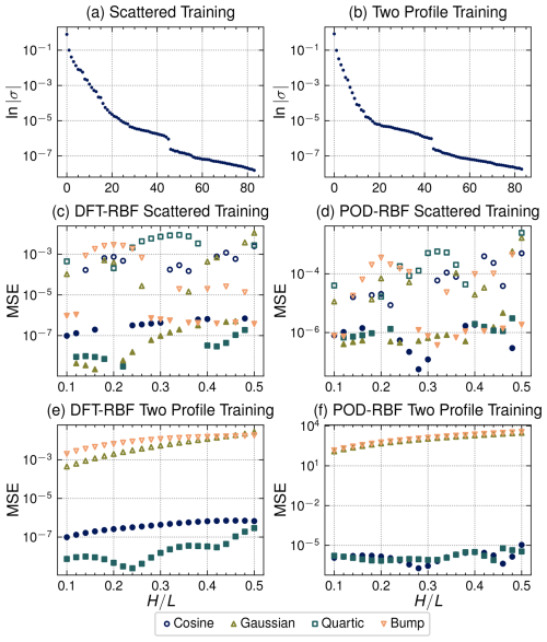
Figure 11 Summary of results for the NIROM-based shear stress perturbation prediction models. Panels (a) and (b) depict the normalized singular values for the training data used to construct the POD basis. Panels (c) and (d) show the MSE for the DFT–RBF and POD–RBF models when using randomly selected cases as training data. Panels (e) and (f) present the MSE when choosing all cases from two profiles as training data. In panels (c–f) filled marks indicate cases used for training where the reported MSE represents the reconstruction error; empty marks represent test cases where the reported MSE represents the prediction error compared to the CFD results.

For the scattered training selection, a random sampling of 40 cases across all four profiles was chosen as the training set. The training cases were used to build the POD basis as well as train the RBF interpolator for both DFT–RBF and POD–RBF. Results for this approach are given in Fig. 11c and d. As to be expected, the highest errors occur for points farthest from neighboring cases of the same profile and for extrapolation at the edges of the case domain. Furthermore, while the DFT–RBF approach achieves better reconstruction errors on average, the POD–RBF results offer a slight improvement in predicting unseen values of $H/L$ over the DFT–RBF.

The second training selection criteria consisted of using all cases from two profiles as training data while predicting on the unseen profiles (see Fig. 11e and f). This allowed us to explore the generalizability of the NIROM methods to unseen topography shapes rather than just unseen parameters as in the first scenario. For this experiment, the DFT–RBF results in Fig. 11e far outperform the POD–RBF results in Fig. 11f. This is most likely due to the less universal nature of the POD basis, which is constructed purely based on the training data and is unable to accurately represent both the input topography and shear stress perturbation for completely unseen profiles. On the other hand, since the DFT basis is not dependent on the data being examined, it is capable of representing the unseen topography and the error is due to extrapolating the input–output relationship to unseen profiles.

5 Discussion

5.1 Intercomparison of shear stress predictions

Thus far we have analyzed the differences in surface shear stress perturbation predictions between an established analytical model, namely KSH, CFD simulations, and data-driven approaches. We have shown that KSH generally overpredicts the extrema compared to an RNG k−ϵ RANS formulation for a range of two-dimensional dune profiles. Errors increase with increasing $H/L$ and have been shown to be correlated with topography slope regardless of the overall dune dimensions. Furthermore, we have explored two data-driven methodologies as avenues for improving computationally efficient models compared to resource-intensive CFD simulations. These various simulations and approaches were compared through the lens of assessing existing capabilities and alternative options for resolving spatial wind and bed shear stress calculations within existing process-based aeolian sediment transport models.

Having examined each of the shear stress perturbation prediction models individually, all of the results are gathered in Fig. 12 in order to discuss their relative performance. It can be seen that KSH is outperformed by all of the trained models for the range of $H/L$ ratios and profiles considered, except for the POD–RBF 2 × 2 results. This result is not too surprising since each of the alternatives was optimized for this specific dataset during training. Concerning the SR results, the expression trained only on the medium set of $H/L$ values, i.e., PySR Med, outperforms that trained only on large $H/L$ values, i.e., PySR Large; however, the prediction error becomes more similar as $H/L$ increases, with PySR Large gaining a slight advantage for the bump and quartic profiles. Overall, the SR results for the medium case set confirm the validity of linearized, asymptotic representations such as KSH while representing a modest improvement due to an optimized prediction of A and B in agreement with Charru et al. (2013). The impact of these modest differences on morphological predictions is discussed further in the following section. However, as demonstrated by the PySR Large results, work is still needed for reducing the error for larger values of $H/L$ and for capturing the distribution of surface shear stress in regions of flow separation.

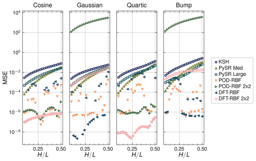
Figure 12 MSE for all shear stress perturbation models grouped by profile. The POD–RBF 2 × 2 and DFT–RBF 2 × 2 results refer to the two profile-trained models. Filled marks indicate cases used for training where the reported MSE represents the reconstruction error; empty marks represent test cases where the reported MSE represents the prediction error compared to the CFD results.

Linear, projection-based, non-intrusive, reduced-order modeling approaches were able to further reduce the prediction error at the cost of generalizability to unseen cases. For the NIROM approaches, scattered training, which covers the entire data space, performs best. Prediction errors are largely dependent on the distance from training cases, and in the case of POD–RBF 2 × 2, the model is unable to generalize to unseen profiles, which poses a challenge for real-world applications where topography evolves with time. Compared to the SR results, the prediction errors are no worse and exhibit significant improvement for high $H/L$ values, especially when unseen cases fall close to seen cases as is true for the bump profile. The success of the simple NIROM approaches in this region, and in particular the DFT–RBF variant, suggests that data-driven methodologies may be able to provide fast prediction models which accurately capture separation effects.

5.2 Error implications for morphological prediction

For theoretical applications of aeolian landform evolution, the exact magnitude of transport rates matters less than capturing the patterns that lead to sediment transport gradients that spur net landform changes. Numerical tools, largely using the KSH approximation, have yielded the ability to synthesize complex two- or three-dimensional topographic change patterns and behaviors as observed in nature (e.g., Durán et al., 2010; Kombiadou et al., 2023). Yet, limited field-scale validation exists in terms of these behaviors. Increasingly, there is a push for more engineering-oriented capabilities that rely on appropriately simulating relevant physical phenomena that necessitate accurate prediction of spatiotemporal rates of sediment mobilization and transport. Ultimately, sediment transport rates are driven by excess shear above a threshold to initiate grain motion. Numerous formulations for aeolian sediment transport exist in the literature, many but not all of which (Martin and Kok, 2017) express the sediment flux (q) as a nonlinear function of u_* or τ. For example, the commonly used modified Bagnold equation (Bagnold, 1937) defines sediment flux as

$$\begin{array}{}\text{(21)}& q=C{\displaystyle \frac{{\mathit{\rho }}_{\mathrm{a}}}{g}}\sqrt{{\displaystyle \frac{d}{D}}}(u_{*}-u_{*,\mathrm{t}}{)}^{\mathrm{3}},\end{array}$$

where ρ_a is the air density, g is gravity, d is the grain size, and D is a reference grain size. $u_{*,\mathrm{t}}$ is the threshold shear velocity for initial grain motion, which may be estimated as

$$\begin{array}{}\text{(22)}& u_{*,\mathrm{t}}=A\sqrt{{\displaystyle \frac{{\mathit{\rho }}_{\mathrm{g}}-{\mathit{\rho }}_{\mathrm{a}}}{{\mathit{\rho }}_{\mathrm{a}}}}}gd,\end{array}$$

where A is a coefficient related to sediment distribution spread and ρ_g is the grain density.

Given that τ and corresponding u_* profiles over dune topography are highly nonuniform resulting from flow acceleration, deceleration, and separation bubble effects and that deviations in KSH from the CFD model results are often not insignificant, this has important implications for the resulting potential for aeolian transport across the dune face.

To directly assess rates of transport and corresponding bed elevation change patterns, we use KSH and PySR outputs as input hot-start files to the AeoLiS (Hoonhout and de Vries, 2016) model for select simulations. On the upwind end of the domain, CFD and PySR outputs both indicate biased higher τ relative to KSH at the base of the dune (e.g., Fig. 13e, f). As spatial gradients in sediment transport result in net bed elevation change, this local reduction in shear results in a small zone of deposition. For the H=6 m, L=25 m case for τ=0.6 Pa, KSH results in about a 75 % larger deposition height at the base of a Gaussian-shaped dune. As previously noted, deviations between KSH and PySR are generally larger on the dune itself, with maximum differences occurring at the crest of the dune form. Assuming bare sand conditions (i.e., no vegetation), spatial gradients in τ predicted by both KSH and PySR result in increasing q across the dune face and therefore a net landward migration of the landform. However, assuming the CFD-based PySR results better represent the true wind flow dynamics, Fig. 14 shows the excess net landward sediment transport across the dune crest from the two spatial shear stress models. Notably, as the wind conditions become more energetic or as the $H/L$ ratio increases, errors associated with the magnitude of sand transport increase. For a given boundary τ, these $H/L$ versus KSH–PySR model differences follow an exponential relationship (Fig. 14).

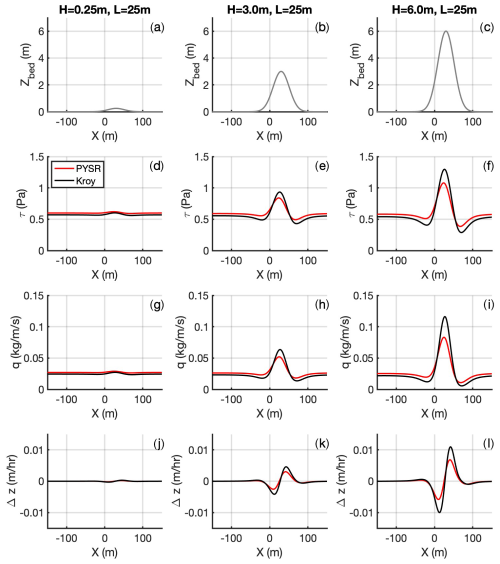
Figure 13 Example differences in predicted aeolian sediment transport fields (g–i) and bed elevation change (j–l) from KSH and PySR for τ= 0.6 Pa for $H/L$ ratios of 0.01 (a, d, g, j), 0.12 (b, e, h, k), and 0.24 (c, f, i, l) Gaussian-shaped profiles.

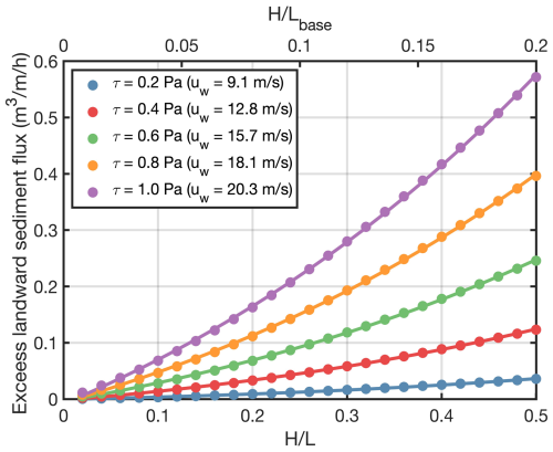
Figure 14 Net differences in simulated sediment flux past the dune crest between KSH and PySR for various $H/L$ conditions (Gaussian-shaped dune) and boundary τ. Dots represent simulated AeoLiS cases and lines reflect the best-fit exponential curve through data points. For linkage to Fig. 1, L_base=2.5L is assumed.

Taken in sum, mis-characterization of the shear distribution across the dune profile has important implications for accurately simulating coastal landform change in terms of both the shape and rate of change. CFD is generally too computationally demanding to couple with aeolian transport models, requiring surrogate or simplified modeling. Given that SR shows the ability to recreate the KSH form for simplified geometries and improve upon flow errors, SR-type approaches could potentially play an important role for improving process-based numerical modeling tools for landform evolution that are required for engineering and design needs. Such approaches are particularly important given that ∼ 99 %, 93 %, and 63 % of coastal dunes from the database in Fig. 1 have $H/L$ ratios exceeding 0.1, 0.2, and 0.5, respectively, assuming L_base= 2.5 L. However, these findings are likely to also have broad implications for landform modeling in other arid (e.g., Tsoar, 2001; Parteli et al., 2014) or extraterrestrial settings (e.g., Atwood-Stone and McEwen, 2013; Parteli and Herrmann, 2007) where slope angles can similarly locally approach the angle of repose.

5.3 Synthesis and remaining challenges

Symbolic regression was able to discover an expression similar to KSH that offers an order of magnitude improvement in prediction error when compared to CFD; however, it still suffers from many of the same issues as KSH, namely, that the error increases with increasing $H/L$, and is unable to capture the effects of separation. Linear, projection-based, non-intrusive, reduced-order modeling approaches were able to further reduce the prediction error at the cost of generalizability to unseen cases. While we were able to obtain modest prediction improvements, we recognize that several challenges remain.

First, in this study we only considered a single value of $L/z_{\mathrm{0}}$ which controls the value of the model constants in KSH and would most likely play a role in any alternative discovered model. Future efforts should extend the dataset to include a range of $L/z_{\mathrm{0}}$ in order to try to extract a relation governing the SR-discovered model coefficients. Only then could the expression be incorporated into existing coastal dune evolution models in a general sense.

Second, we have not considered the effects of vegetation within this study. Steeper coastal foredunes are often vegetated, resulting in reduced shear at the sand surface. This somewhat reduces the concern of errors for steep dunes as the surface shear often drops below the transport threshold; however, in many models the effect of vegetation is applied as a correction factor to the topographically driven shear stress perturbation as in Durán and Moore (2013). Therefore, seeking to increase the accuracy of predictions of τ^′ over the equivalent unvegetated surface for steep dunes is still warranted.

Third, while the NIROM approaches show promise, especially if data are available that sufficiently cover the range of dune topographies expected for a given scenario, concern for their ability to generalize to unexpected topographies which may arise over the course of a dune evolution simulation remains. However, other techniques, such as the use of nonlinear auto-encoders to determine the reduced basis representation and deep learning methods for capturing the latent space mapping from input to output, may provide viable alternatives with improved generalization (Maulik et al., 2021; Dutta et al., 2022).

Finally, we have focused exclusively on simple, idealized two-dimensional dune profiles and have not considered more complex transects that may experience multiple areas of separation such as can occur with severely scarped profiles. Furthermore, real-world coastal dunes are inherently three-dimensional and experience a variety of wind directions and complex, three-dimensional flow effects such as topographic steering and recirculation (e.g., Smyth et al., 2012; Piscioneri et al., 2019). A not insignificant amount of work would be required to extend these approaches to three-dimensional dunes considering the increased computational expense for generating 3D CFD simulation data, as well as considering topographic variations in an additional dimension. However, the methodologies themselves should be directly applicable given data availability.

6 Conclusions

Coastal dunes represent an important line of defense against storm-related flooding hazards. As such, accurate models for predicting their evolution over relevant engineering timescales is paramount for future risk assessments and the development of engineering solutions. Current process-based models make use of linearized analytical solutions to the underlying governing equations which, while easy to implement and computationally efficient, have known deficits for steep topographies. This work highlights that the KSH form widely used in existing tools performs well for the low-slope dune shapes for which the analytical formulation is designed. On dune forms with steeper topography and higher $H/L$ ratios, errors in the magnitude of bed shear stress predictions – compared to CFD model predictions – increase across the dune face. These errors are typically largest at the dune crest, the ramification of which is that existing formulations result in a faster net landward migration of the dune form in morphological models than would be expected. Overall, we have provided an analysis of the limitations of existing analytical prediction models for airflow over coastal dunes and presented two data-driven approaches for constructing alternative fast prediction methods that reduce error relative to the KSH approach. The various newly presented approaches reduce the global error of stress predictions and/or improve on the ability to simulate patterns in complex flow dynamics not fully resolved by the analytical solution. While the improvements presented do not yet provide a complete solution for flow predictions across all dune forms, this work both highlights existing limitations in current dune modeling frameworks and demonstrates new methodologies that could enable more reliable predictions of spatial bed shear stress patterns in the full range of $H/L$ conditions observed in natural coastal systems.

Appendix A: Symbolic regression details

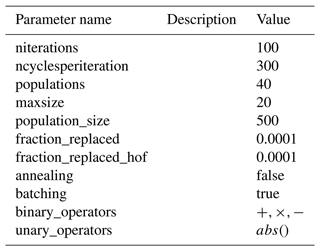
This appendix provides additional details for symbolic regression results. PySR hyperparameters that were changed from their default values are provided in Table A1. These values were tuned to provide robust results across all of the noisy KSH-generated data and used in subsequent PySR runs.

An exhaustive list of the expressions returned by PySR when provided KSH-generated data with Gaussian noise is provided in Table A2. In some cases, some basic simplification or regrouping of the expressions has been performed.

Table A1 Robust parameters for PySR.

Table A2 Simplified PySR discovered expressions for various SNRs. In the interest of space $\widehat{\cdot }$ symbols indicate Fourier-transformed values.