Spatial assessment of sediment production in a badland catchment using repeat LiDAR surveys, Draix, Alpes de Haute-Provence, France

With denudation rates locally exceeding one centimetre of weathered marl per year, i.e., more than 200 T ha⁻¹ yr⁻¹, the badlands of the Durance basin in the French Alps are one of the most eroding areas in the world. Since 1983, the Draix-Bléone Observatory has been using hydro-sedimentary stations to monitor several of these small, unmanaged badland catchments, where the hydrological response to seasonal storms is rapid and intense. In order to fingerprint soil loss in the 86 ha Laval basin, we combine outlet records with an analysis of airborne and UAV LiDAR data taken over a 6-year period, alongside a bulk density model to account for porosity variations with depth and drainage network reconstruction. This allows us to map mass movements and determine a sediment budget at catchment scale. We find that landslides and crest failures represent very active areas, accounting for at least 15 % of the watershed's sediment budget throughout the period under study, despite affecting only 1 % of the bare surfaces. They contribute to the high erosion rates observed in low-drainage areas, with up to two centimetres of fresh marl lost per year, 3.5 times the average value on the rest of the bare slopes. Despite certain methodological constraints, our approach seems very promising at identifying local erosion hotspots, quantifying their contribution to the sediment budget and assessing sediment transport across geomorphological units. It could also be adapted to time series and more detailed identification of geomorphic processes in order to monitor the dynamics of badland catchments in a changing climate.

1 Introduction

Badlands are highly erosive landscapes with a dissected, ravine-like morphology that is largely devoid of vegetation (Bryan and Yair, 1982; Harvey, 2004). They generally develop in semi-arid regions and, to a lesser extent, in humid and sub-humid regions, where the lithology is fragile and highly sensitive to climatic events (Gallart et al., 2002, 2013). The Draix Terres Noires, in the southern French Alps, are one such area. They result from successive gullying phases (Descroix and Gautier, 2002; Moreno-de Las Heras and Gallart, 2018) that began at the end of the Pleistocene and are linked to post-glacial climate changes (De Ploey, 1991; Clément, 1996). However, they only took on their current badland form during the Little Ice Age (15th–19th centuries), as a result of intensive agro-pastoral practices (Ballais, 1997). While some hillslopes were reforested at the end of the 19th century (in Le Brusquet catchment, for example), others remain mostly unvegetated and are subject to high erosion rates, reaching up to one centimetre of weathered marl per year, as in the Laval catchment, where this study is conducted (Mathys et al., 1996; Vallauri, 1997).

Numerous studies have been carried out on these badlands at plot scale (1–100 m²) on bare slopes to analyse the interactions between rainfall, runoff and erosion under controlled conditions, and in particular to describe the hydro-sedimentary processes associated with Hortonian runoff or subsurface infiltration (e.g. Wijdenes and Ergenzinger, 1998; Mathys et al., 2005; Garel et al., 2012). In parallel, high-resolution topography (HRT) acquisition methods are becoming more widely available to geomorphologists (e.g. Lague et al., 2013; Neugirg et al., 2015; Passalacqua et al., 2015). Using a terrestrial laser scanner (TLS), Bechet et al. (2015) were able to observe small hillslope processes such as regolith swelling, crack closure, micro-landslides and the initiation of miniature debris flows (MDFs) at the millimetre scale on such plots. However, if the plot scale is too small relative to the average transport distance of entrained material, the analysis may be unrepresentative and fail to capture the full contribution of primary sediment sources (Kinnell, 2009; Boix-Fayos et al., 2006; Yair et al., 2013). Consequently, the experiment carried out by Bechet et al. (2015) was reproduced by Bechet et al. (2016) on the 0.13 ha Roubine catchment, which is adjacent to the Laval catchment. This allowed the seasonal dynamics of erosion to be observed in detail, in a transport-limited erosion regime in winter and a supply-limited regime in summer. Using dendrochronology to calibrate a slope-erosion relationship alongside a high-resolution topographic reconstruction with UAV LiDAR, Saez et al. (2011) were also able to produce the first map estimating the spatial distribution of erosion rates in the Laval catchment. Similar studies have been conducted using TLS surveys in the Spanish Central Pyrenees (Vericat et al., 2014; Nadal-Romero et al., 2015), as well as in the biancane and calantchi badland formations in Italy (Neugirg et al., 2016; Marsico et al., 2021). Apart from these notable exceptions, studies conducted at catchment scale in the Draix area have primarily focused on investigating and modelling the complex relationship between sediment export and climatic variables (Mathys et al., 2003; Badoux et al., 2012; Taccone et al., 2018; Carriere et al., 2020; Ariagno et al., 2022; Roque-Bernard et al., 2023) or (re)vegetation (Rey, 2003; Burylo et al., 2011; Erktan et al., 2013; Carriere et al., 2020).

However, erosion mechanisms scale up in a highly nonlinear way with increasing drainage area due to the competing effects of increased gully connectivity and sediment storage, as well as a change in the slope distribution that dominates erosive processes (De Vente and Poesen, 2005; Puigdefábregas, 2005; Vanmaercke et al., 2011). For instance, the Laval catchment (86 ha) and the Roubine catchment (13 ha) are neighbours with similar environmental conditions and forcings, yet the Laval sediment flux is dominated by suspended sediment contribution, while the Roubine sediment flux is dominated by bedload contribution (Le Bouteiller et al., 2024; Klotz et al., 2023). To assess the relationship between drainage area and sediment export, Nadal-Romero et al. (2011) analysed 16 571 annual export values at plot and catchment scale from 87 Mediterranean badland sites. They observed high and highly variable sediment export for drainage areas < 10 ha, followed by a power-law decrease in sediment export with drainage area for larger areas. This deviation from the De Vente and Poesen (2005) model for Mediterranean environments shows that, while seemingly ideal natural laboratories, badlands have an intrinsic complexity (Yair et al., 2013; Nadal-Romero and García-Ruiz, 2018). This result was obtained in configurations with strong vegetation and climatic contrasts, as well as different monitoring methods. Some of these methods, such as gauging stations, are considered more reliable than others, such as runoff plots or erosion pins, which are more widely used (Nadal-Romero et al., 2011). The limitations of the existing sediment yield assessment monitoring methods call for a multi-scale study that spatially identifies soil loss using a unique, non-invasive measurement method and quantitatively analyses topographic changes.

Airborne remote sensing methods are often used to inventory local sediment sources, estimate their volume, and evaluate their contribution to overall catchment erosion (e.g. Guzzetti et al., 2012; Bechet et al., 2016; Krenz and Kuhn, 2018; Bernard et al., 2021). In the case of landslides, this is facilitated by empirical area-volume relationships (e.g. Guzzetti et al., 2009; Larsen et al., 2010; Parker et al., 2011; Li et al., 2014; Massey et al., 2020; Alberti et al., 2022; Yunus et al., 2023), as well as the advent of photogrammetric methods based on aerial photographs (e.g. D'Oleire-Oltmanns et al., 2012; Krenz and Kuhn, 2018; Lucas and Gayer, 2022). More recently, airborne LiDAR systems (e.g. Bull et al., 2010; Passalacqua et al., 2015; Okyay et al., 2019; Bernard et al., 2021) have made it possible to reconstruct the topography of entire basins at high resolution while overcoming slope obstructions (Brodu and Lague, 2012; Stöcker et al., 2015; Neugirg et al., 2015). However, to date, such studies have estimated the volumes of sediment sources and sinks without assessing their corresponding masses (Neugirg et al., 2015; Krenz and Kuhn, 2018; Bernard et al., 2021), thus failing to take into account the variations in compaction associated with erosive processes such as landslides (Chen et al., 2005; Bernard et al., 2021). These variations in porosity can be significant, particularly in badlands where the ratio of the bulk density of disaggregated colluvial deposits at the foot of slopes to that of unweathered marl is 1 : 2 (Mathys et al., 1996). Furthermore, these approaches usually evaluate topographic changes using Differences of DSMs (DoDs), which are generally less accurate than direct point cloud comparisons in regions with complex terrain (Lague et al., 2013; Bernard et al., 2021).

This study aims to explore the potential of multi-temporal LiDAR surveys to spatially resolve sediment production, defined as the initial mobilisation of weathered material, in the Laval experimental basin. It also aims to establish a relationship between this process and the sediment export measured at the outlet gauging station. Section 2 describes the study area and presents the gauging station, LiDAR data, and density measurements. Section 3 describes the procedure for mapping mass movements within the drainage network and performing a sediment budget, which is defined as a mass balance for an open system at catchment scale. Due to the complex topography of the study area, the core of the proposed method is a direct comparison of the 3D point clouds from the LiDAR surveys. Section 4 evaluates the contribution of the inventoried sediment sources and sinks to the erosion dynamics of the watershed and its geomorphological units, which are defined based on specific drainage areas (i.e., the drainage area per unit flow width) (Bernard et al., 2022). Finally, Sect. 5 discusses interpretations of these results, estimates production rates in different geomorphological units and examines the suitability of the methodology for assessing badland erosion processes across spatial and temporal scales in a changing climate.

2 Study site and data

2.1 The Draix-Laval experimental basin

2.1.1 The Laval's Terres Noires

The Laval catchment is a marly, torrential watershed spanning 86 ha, more than 60 % of which are gullies and steep, bare slopes (typically 40–50°), which are characteristic of badlands. Located between 850 and 1250 m in the Bléone valley, it lies near the town of Draix and upstream from Digne-les-Bains in the Alpes de Hautes-Provence region (Fig. 1).

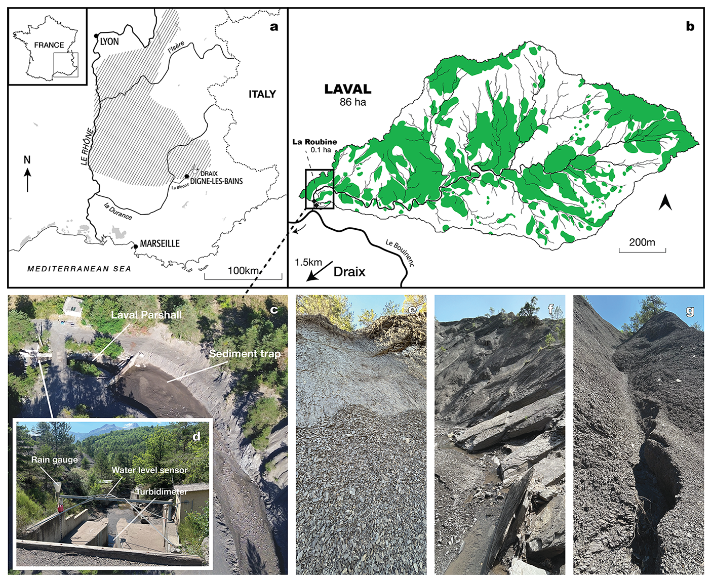
Figure 1 Map showing (a) the extent of the “Terres Noires” in the French Alps, represented by hatching (adapted from Antoine et al., 1995), and (b) the Laval basin, located 1.5 km northeast of Draix, with its drainage network and vegetation cover shown in green. (c) Catchment outlet with the sediment trap and hydro-sedimentary monitoring station. (d) Detail of the instrumentation used at the monitoring station. Examples of geomorphological processes observed on the crests (e), slopes (f), and gullies (g) are also presented.

Draix has a Mediterranean mountain climate, with an annual precipitation of around 900 mm and considerable inter-annual variability (±200 mm). The harsh winters are conducive to the frost-cracking weathering of the Jurassic black marls known as “Terres Noires” (Ariagno et al., 2022). Rainfall in spring and autumn is frequent but not intense, with October being the wettest month at an average of over 120 mm. Storms are frequent in late spring and summer, with an average of five major events per year. Their extreme intensity, exceeding 50 mm h⁻¹ over short periods, is responsible for torrential floods with suspended sediment concentrations of several hundred grams per litre and event-scale sediment export of several hundred cubic metres (Mathys et al., 2005; Ariagno et al., 2022; Klotz et al., 2023). This results in very high interannual variability in sediment export, reaching about half of the total. On a regional scale, the Terres Noires are responsible for almost 40 % of the sediment load of the Durance, despite representing only 1.2 % of its catchment area (Copard et al., 2018).

2.1.2 Draix-Bléone Critical Zone Observatory

The extreme fragility of the Laval black marls and the surrounding basins make them ideal experimental sites for conducting experiments on the erosive processes of humid badlands. This is why the INRAE (French National Research Institute for Agriculture, Food and Environment) has been monitoring these basins since 1983 and, since 2000, as part of the Draix-Bléone Critical Zone Observatory (CZO). In 2015, the latter joined the OZCAR research network (Gaillardet et al., 2018, http://www.ozcar-ri.org, 29 October 2025), which is dedicated to studying the critical zone, the near-surface Earth layer extending from groundwater table up to the top of the vegetation canopy.

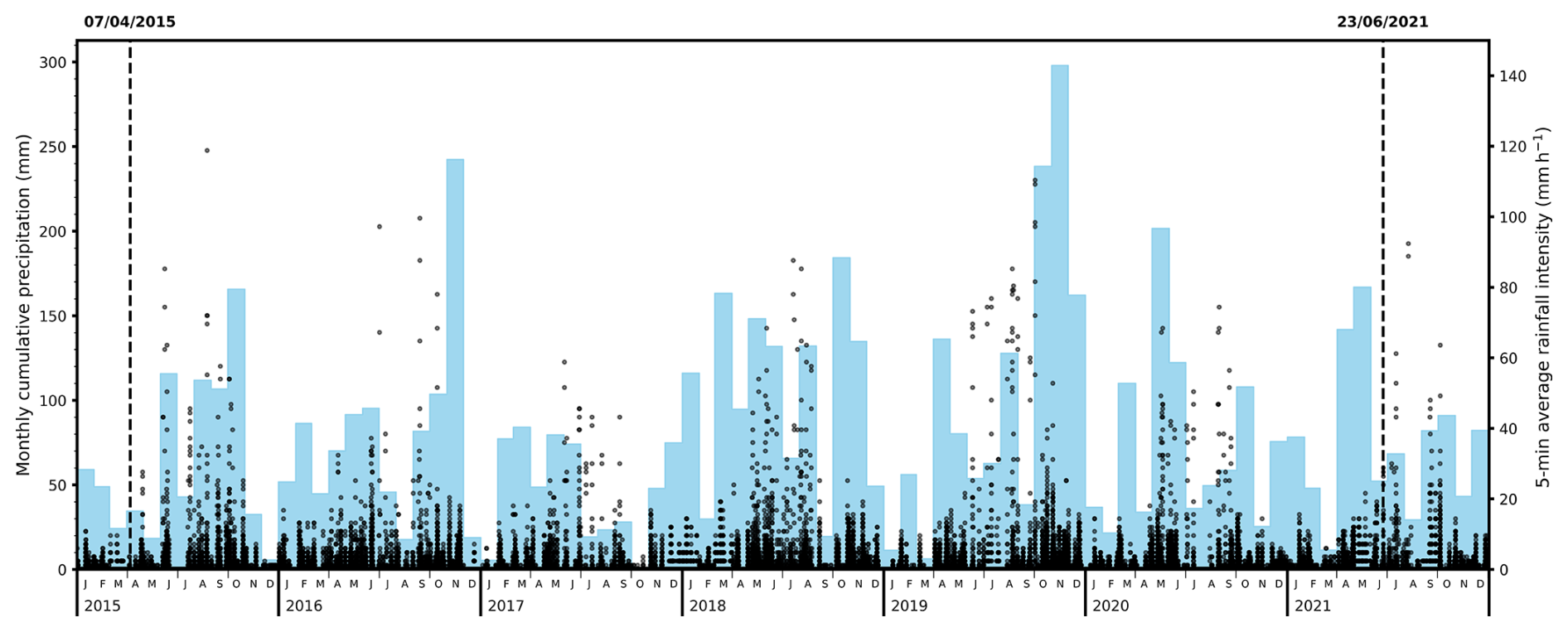
Figure 2 The monthly cumulative precipitation (mm) and 5 min average rainfall intensity (mm h⁻¹) recorded at the meteorological stations in the Laval basin between 2015 and 2021.

A hydro-sedimentary station has been installed upstream of the confluence of the Laval ravine and the Bouinenc, a tributary of the Bléone river (see Fig. 1). It consists of a tipping bucket rain gauge and a water level sensor that makes indirect measurements of the flow discharge at 10 s intervals in a Parshall flume. The station is also equipped with automatic water samplers that can take samples at intervals of up to one minute, as well as an an optical fibre turbidimeter that measures suspended sediment concentrations at 10 s intervals. The typical particle sizes measured are 5 to 20 µm (D₅₀) and up to 20 to 90 µm (D₉₀). The coarsest materials that make up the bedload are deposited in the 1400 m³ sediment trap, which is emptied once or twice a year. Topographic surveys of the trap are conducted after each intense event to measure the contribution of the bedload to the total sediment export. All data from the Laval station, as well as from the other Draix-Bléone catchments, are described in Klotz et al. (2023) and are available in the BDOH database repository (Le Bouteiller et al., 2024). Figure 2 summarises the rainfall data recorded between the two LiDAR surveys in April 2015 and June 2021. Approximately 33 intense rainfall events occurred between the two surveys, 25 of which took place between May and August.

2.2 LiDAR campaigns

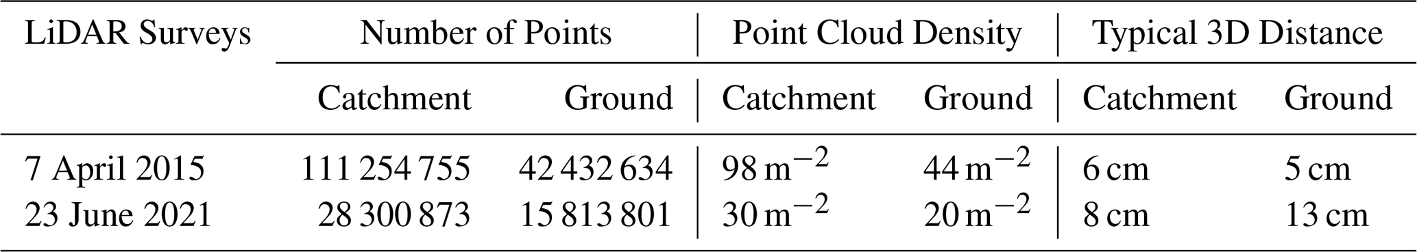
A high-spatial resolution study of the topography of the Laval basin was carried out using two LiDAR surveys between 2015 and 2021. Table 1 summarises the characteristics of the two point clouds.

Table 1 Point cloud characteristics for the 2015 and 2021 airborne LiDAR campaigns, including the whole catchment points and for the ground point subset.

2.2.1 UAV LiDAR survey (7 April 2015)

An initial survey was carried out on 7 April 2015 as part of the OSUG@2020 LabeX supported project (Le Bouteiller, 2025). The Laval basin was scanned by the Sintégra company using an RIEGL LMS-Q680i full-waveform LiDAR system mounted on a UAV helicopter.

The resulting point cloud is certified, georeferenced, and classified as either ground or above ground. The altimetric accuracy is estimated to be 3 cm, based on 30 GPS measurements acquired over two control surfaces. Although the nominal planimetric accuracy is 20 cm, the error is probably smaller given that the nominal altimetric accuracy is 10 cm.

2.2.2 Airborne IGN LiDAR HD survey (23 June 2021)

The LiDAR HD programme, led by the French National Institute of Geographic and Forestry Information (IGN), aims to provide free access to 3D maps of metropolitan France and its overseas departments and territories (excluding French Guiana) with an accuracy of 10 cm by the end of 2025 (IGN, 2024). While the entire country is not covered by the programme yet, the Draix Bléone CZO catchment area was observed on 23 June 2021 at 07:34 UTC. The LIDAR system is mounted on an aircraft and uses a tilting mirror to acquire data in bands.

The data is georeferenced in the Lambert 93 coordinate system, with cloud segmentation applied using IGN's myria3D deep learning algorithm to distinguish between ground, vegetation and buildings (Gaydon, 2022). According to the programme specifications, the minimum accuracy (RMS) is 10 cm for altimetry and 50 cm for planimetry.

2.3 Density measurements

In the sediment trap, a dry density value of 1.7 g cm⁻¹ is used to estimate the mass of material deposited, with volumes measured by topographic surveys after a storm event (Klotz et al., 2023). However, measurements carried out in 2001 in the Roubine trap, adjacent to the Laval basin, yielded an average value of 1.5 g cm⁻¹ (Mathys, 2006). This study repeats the density measurements, this time at various sites in the Laval catchment, primarily in sediment deposits along the channel and its banks, as well as in colluvium at the bottom of slopes and gullies. The experimental protocol is as follows:

1. Sampling a sediment deposit using an 11 L bucket;

2. Weighing the sample using a hook balance;

3. Placing 3D-printed reglets around the sample area as scale references for photogrammetry;

4. Photographing the sample area from different angles;

5. Sampling a portion of the deposit using a vial;

6. Measuring the wet/dry weight before and after 48 h of oven drying, and determining the initial water content of the sample;

7. Estimating the in situ volume of the sample by photogrammetry based on the photographs taken in the field;

8. Calculating the dry density of the deposit from the measured mass, occupied volume and estimated water content χ, with ${\mathit{\rho }}_{\mathrm{dry}}={\mathit{\rho }}_{\mathrm{wet}}/(\mathrm{1}+\mathit{\chi })$.

The measurement uncertainties include those related to the weight of the sample taken from the 11 L bucket, the volume measurement, and the water content χ. A value of 10 % can be assumed for the weight, while the volume uncertainty is typically 100 mL, i.e., about 2 % of the volume. Consequently, the wet density values are known within an average range of 0.2 g cm⁻¹. The water content could not be determined for all samples. Values measured in March 2024 ranged from 11.96 % to 15.65 %, with corresponding reductions in dry density from 86.5 % to 89.3 %. Where the water content was not measured, a value of 14 ± 10 % was assumed. This gives an average uncertainty in the dry density values of 0.25 g cm⁻¹.

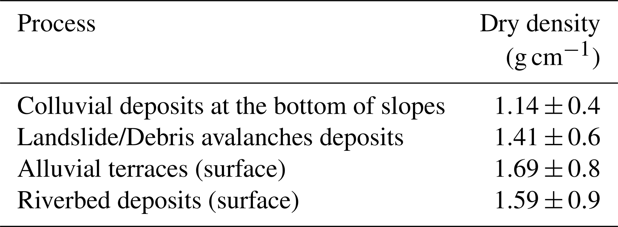
Density measurement campaigns were carried out in the sediment deposits of the Draix Laval basin in March and June 2024. In March, the water content of the samples was measured, while in June, a mean value of 14 % was used, with an error margin of 10 %. Table 2 shows the density measurements according to the geomorphological processes involved. Colluvial deposits have particularly low densities, and landslide material is also significantly less dense than that found in the channel bed or on the riverbanks.

Table 2 Measurements of dry density using geomorphological processes.

3 Method

The availability of two high-resolution LiDAR surveys that cover the entire Laval basin alongside hydro-sedimentary records from the outlet and density measurements, provides an opportunity to assess sediment production in a spatially distributed manner. The workflow involves a detailed analysis of topographic changes carried out directly on the 3D point clouds. These are then projected onto a regular grid to estimate the corresponding volumetric changes, which are converted into mass changes using sediment density measurements.

3.1 LiDAR topographic change assessment

The volumetric changes derived from multi-temporal LiDAR surveys are assessed through a three-step process. This process is described below and summarised in Fig. 3.

Figure 3 Workflow for assessing volumetric changes of the topography using point cloud data.

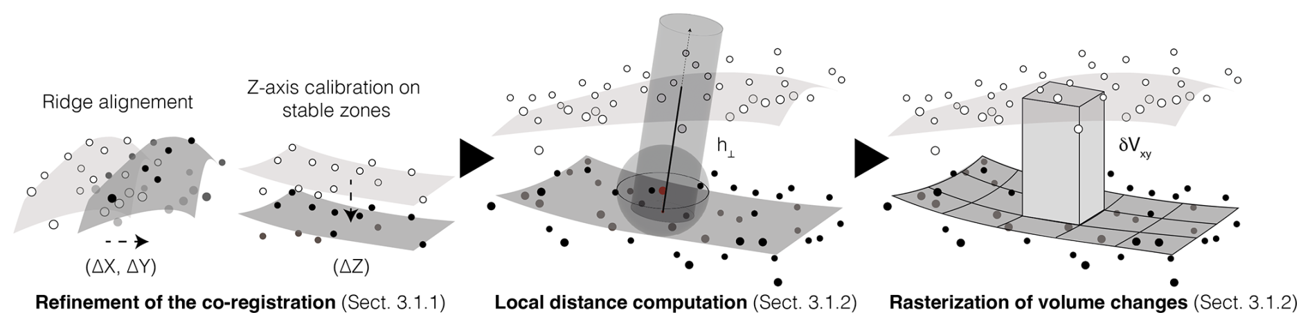
3.1.1 Refinement of the co-registration of the campaigns

Co-registration of LiDAR campaigns is a major source of systematic error. For example, a shift of one centimetre in the z-axis between point clouds of an 86 ha catchment area will lead to an over- or underestimation of the total volume by 8600 m³. Systematic errors in co-registration can also occur in the horizontal plane, leading to ridge misalignment. In this study, we refine the point cloud co-registration by analysing the distribution of local 3D distances between the campaigns' point clouds on subsets of the catchment area. We focus on nearly stable flat surfaces to identify vertical errors and on slopes with simple geometry to align ridges. The method used to compute local 3D distances is detailed in Sect. 2.2.2, and further information on the co-registration is provided in Fig. D1. We show that a relative shift of approximately $(\mathrm{\Delta }X,\mathrm{\Delta }Y,\mathrm{\Delta }Z)=(\mathrm{10},\mathrm{11},\mathrm{0.5})$ cm, of the order of the distance between neighbouring points within a cloud, must be applied to the 2021 campaign to enable accurate multi-temporal analysis with the 2015 campaign. The absolute planimetric and altimetric uncertainties presented in Sect. 2.2 are reduced to $(\mathit{\delta }X,\mathit{\delta }Y,\mathit{\delta }Z)=(\pm \mathrm{5},\pm \mathrm{5},\pm \mathrm{1})$ cm in the relative position between clouds. This also reflects the internal accuracy of the point clouds.

3.1.2 Local distances between the point clouds

The evolution of the topography from one campaign to the next is assessed by calculating the local distances h_⟂ between the corresponding clouds along the normals to the source surfaces. This is achieved using the M3C2 (Multiscale Model to Model Cloud Comparison) method, developed by Lague et al. (2013), which considers the local roughness scales of complex natural surfaces. By studying LiDAR data and aerial photographs of the Super-Sauze landslide in the Ubaye Valley in the Alpes de Haute-Provence region, which is also composed of Jurassic black marl, Stumpf et al. (2015) have demonstrated that this method is an accurate and versatile tool for analysing these active areas. It outperforms DoD (Difference of DSMs) methods, as well as point-to-point and point-to-mesh measurements (Stumpf et al., 2015). As the point clouds for the 2015 and 2021 campaigns distinguish between vegetation/structures and ground points, only the latter sub-cloud is used for each campaign in our study. Given the complexity of our surfaces and the point densities presented in Table 1, we empirically set the local scale suitable for distance calculation to r=30 cm for both clouds. Uncertainties in local distance computation result from the combined standard deviations of surface normal estimation on the source cloud and local distance measurements with the target cloud (Lague et al., 2013).

3.1.3 Inferring local volume changes

Volumetric variations in topography are mapped by rasterising the resulting point cloud to a 1 m² grid. This enables small mass movements to be captured while accounting for the density of the point clouds and avoiding empty cells. For each grid cell, rasterisation assigns an average value for the different attributes, such as height and local distance. We then construct prisms from this grid, whose volume corresponds to the local variation between the two campaigns. The surface model is used to orientate the base facets according to the topographic gradient, and the local distance between the point clouds determines their height (see Appendix A). The signs of the M3C2 local distances are retained in the volume calculations to indicate whether accumulation or erosion has occurred. Standard deviations are also propagated throughout, enabling us to estimate the volume uncertainty of each irregular voxel.

3.2 Effective density model of the marls

Land movements in the catchment can lead to local and transient accumulations of matter, whereas the integrating nature of the drainage network implies that, under the assumption of a steady state, all this matter will ultimately be measured at the hydro-sedimentary station. Consequently, a sediment budget is constructed at the catchment scale, considering it as an open system. It should be closed by the export values measured at the station.

To establish the watershed sediment budget and capture the contributions of different erosion modes, it is essential to map (and sum) changes in mass, δM_xy, rather than volume, δV_xy. This can be achieved by using local bulk densities, which cannot be measured directly at the catchment scale and are likely to vary considerably depending on the local material type (e.g., fresh bedrock, regolith, alluvial or colluvial deposits). It also depends on the local history of erosion and deposition.

We have therefore developed a simplified bulk density model based on sediment deposit measurements and marl weathering profiles from other studies. As shown in Sect. 2.3, the dry bulk density of sediment deposits varies considerably due to geomorphological processes. However, for practical purposes, a mean constant value of 1.40 ± 0.3 g cm⁻³ is adopted here. For eroded materials, our model should reflect the marl weathering profile, which varies significantly with depth, as demonstrated by Maquaire et al. (2002) and Rovéra and Robert (2006). The compact marl horizon is typically located at a depth of around 45 cm with a material density reaching up to 2.65 g cm⁻¹ (Lavergne, 1986; Mathys, 2006; Serratrice, 2017). This is overlain by a stratified regolith that is progressively weathered towards the surface, where the density varies seasonally: it reaches a minimum of (1.39±0.2) g cm⁻¹ in winter due to frost-cracking and a maximum of (1.76±0.2) g cm⁻¹ in summer when it is exposed to transport processes during seasonal storms (Ariagno et al., 2023). Accordingly, we define a linear density profile of eroded materials with depth, ranging from 1.6 ± 0.3 g cm⁻¹ at the surface to 2.65±0.3 g cm⁻¹ (not exceeding 2.8 g cm⁻¹) at 45 cm, beyond which it is assumed to be constant.

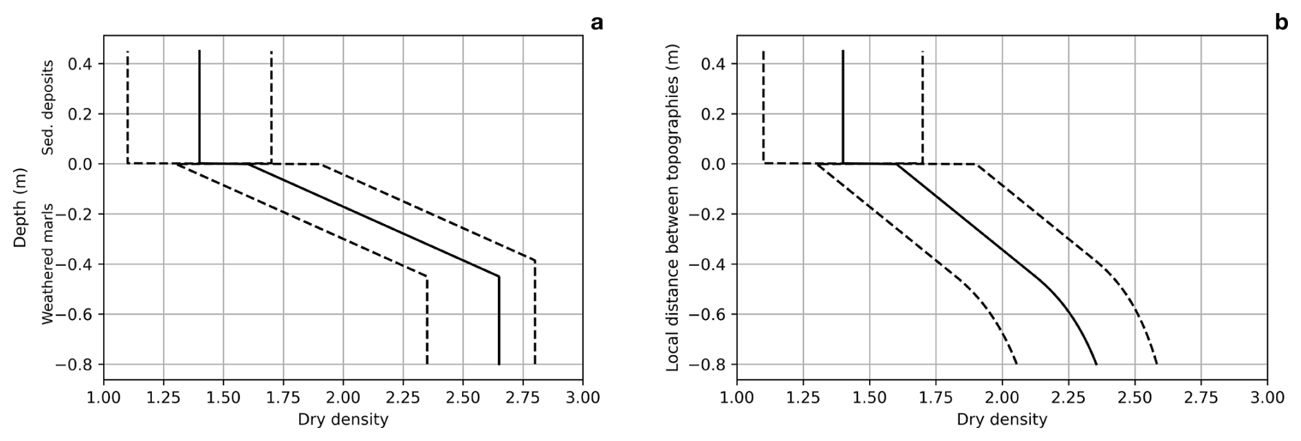
Figure 4 (a) Designed density model ρ(z_⟂) and corresponding (b) bulk density profile ρ_eff(h_⟂) as functions of weathered marl erosion depth $(z_{⟂}<\mathrm{0})$ or sediment deposits depth $(z_{⟂}>\mathrm{0})$, and local distance measured between topographies (h_⟂), respectively. Densities are expressed in g cm⁻¹.

Figure 4a shows the resulting model. In order to incise a layer at a given depth, the upper layers must first be eroded. Thus, at a given local distance h_⟂ measured between the local surfaces of two surveys corresponds an effective density ${\mathit{\rho }}_{\mathrm{eff}}={\int }_{\mathrm{0}}^{h_{⟂}}\mathit{\rho }\left(z_{⟂}\right)\mathrm{d}{z}_{⟂}$, shown on Fig. 4b. By construction, the resulting profile is framed by two variations of ±0.3 g cm⁻¹ at a given depth, thus providing an upper and lower bound that estimates the associated extended uncertainties. However, this model does not account for the spatial variability of marl deposition and weathering profiles by design.

3.3 Outlet cumulative sediment export

The hydro-sedimentary records are available on the observatory's website (Le Bouteiller et al., 2024). From the discharge and suspended sediment concentration, and the volumes scoured from the sediment trap, converted to tonnes at the measured density of 1.7 g cm⁻¹ (Klotz et al., 2023), we can estimate the total sediment export M_tot. at the station. Table 3 summarises the annual and cumulative export over the sequence, with expanded uncertainties calculated using the quality codes assigned by Klotz et al. (2023, see Appendix B for details). The cumulative export totals 89.0 ± 28.6 kT between April 2015 and June 2021.

Table 3 Annual and cumulative sediment export measured at the catchment outlet between the two LiDAR campaigns. M_susp. and M_dep. are the cumulative suspended matter and deposited sediment in the sediment trap, respectively. M_tot is the sum of these contributions. The years 2015 and 2021 are marked with a ^∗ in the table to indicate that data are reported from 7 April 2015 up to 23 June 2021. Expanded measurement uncertainties are calculated using quality codes assigned to the recorded date (Klotz et al., 2023, see Appendix B for details).

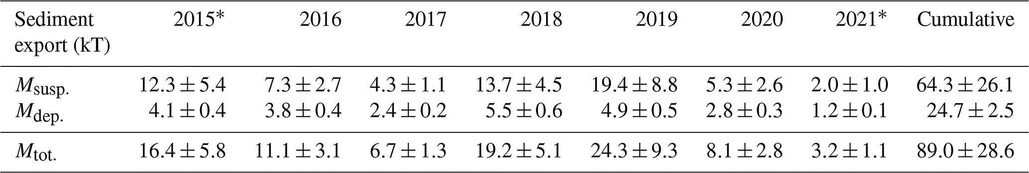
By taking two similar periods, between April 2008 and June 2014 and between April 2012 and June 2018, we obtain a total sediment export of 87.0 ± 26.7 and 87.5 ± 28.8 kT, respectively. Hereafter, we consider the former value to be representative of the basin's behaviour on this timescale, as it is long enough to compensate for the large inter-annual variations.

3.4 Drainage network reconstruction

The following erosion and deposition features will be identified in two ways: by manually labelling sources and sinks and by determining their position within the drainage network.

The labelling of erosion hotspots, to be discussed in the next section, is primarily carried out on the resulting change map, supported by topographic information and interpretation of orthoimages. Five categories will be defined: crest failures, landslide scars, landslide deposits, a natural dam in the main channel, and the sediment trap at the outlet.

To investigate the contributions of each sediment sources and sinks in relation to their location within the basin, we use the GraphFlood algorithm (Gailleton et al., 2024) to reconstruct the drainage network of the Laval catchment under flood conditions, based on the 50 cm DTM derived from the 2015 LiDAR campaign. This algorithm uses graph theory to efficiently solve the 2D shallow water equations, modelling the characteristics of the flow (e.g., flow rate, water height and flow width) under steady-state conditions for given runoff rates. Here we select a high rate of 50 mm h⁻¹, which corresponds to intense rainfall likely to generate sediment transport (Mathys et al., 2005). The method enables us to introduce hydro-geomorphic metrics, such as the specific drainage area (also known as the effective drainage area), which is generally constructed as the ratio of the drainage area to the flow width, estimated from contours. Within this algorithm, it is defined as the ratio of the discharge per unit flow width (specific discharge) to the runoff rate (Bernard et al., 2022; Gailleton et al., 2024). This metric is commonly used in hydrological modelling (Beven and Kirkby, 1979; Bernard et al., 2022) and slope erosion modelling (Moore and Wilson, 1992; Dietrich et al., 1993), or in combination with slope to define the Topographic Wetness Index (TWI) as a proxy for soil moisture (Beven and Kirkby, 1979; Riihimäki et al., 2021). The widespread use of high-resolution digital elevation models, particularly those generated using airborne LiDAR, has made it possible to accurately describe the structure of watercourses and to use this metric, which takes flow width into account (Bernard et al., 2022). Figure 6 presents the resulting map, which is discussed further in the following section.

4 Results

4.1 Erosion and deposition hotspots

Figure 5 shows the local mass changes in the denuded areas of the Laval basin resulting from the workflow described in Sect. 3.1 and 3.2. Vegetated areas are masked using an orthophotography from IGN (2021), as erosion is assumed to be less significant in these areas than in denuded areas (Carriere, 2019; Bunel et al., 2025). Surface reconstruction is also considered to be less reliable in these areas (see Sect. 5.4). The mass variations appear to be unevenly distributed across the basin: 97 % of the bare areas have values between −1 and +1 T m⁻² (approximately ±40 cm of fresh marl), but this represents only 54 % of the total LiDAR sediment budget in denuded areas. This is because significant signals greater than a few T m⁻² are found on slopes, in areas limited to a few tens of square metres. Erosion and deposition signals are generally associated, with the latter extending a few metres downstream of the former. These local movements are sometimes visible on orthoimages constructed from aerial photographs, which supports the interpretation of shallow landslides or debris avalanches. Additionally, when examining the drainage network in Fig. 6 or the topography in a DEM, it is evident that some of the erosion signals are located on the ridges of slopes (< 10⁰ m² m⁻¹ specific drainage area) and are consequently categorised as crest or ridge-top failures. Finally, strong signals above ±1 T m⁻² are also found in the main channel (> 10⁶ m² m⁻¹ specific drainage area), in the sediment trap at the outlet, and 650 m upstream, extending over 200 m. These erosion and deposition hotspots are labelled manually in Figs. 5 and 6.

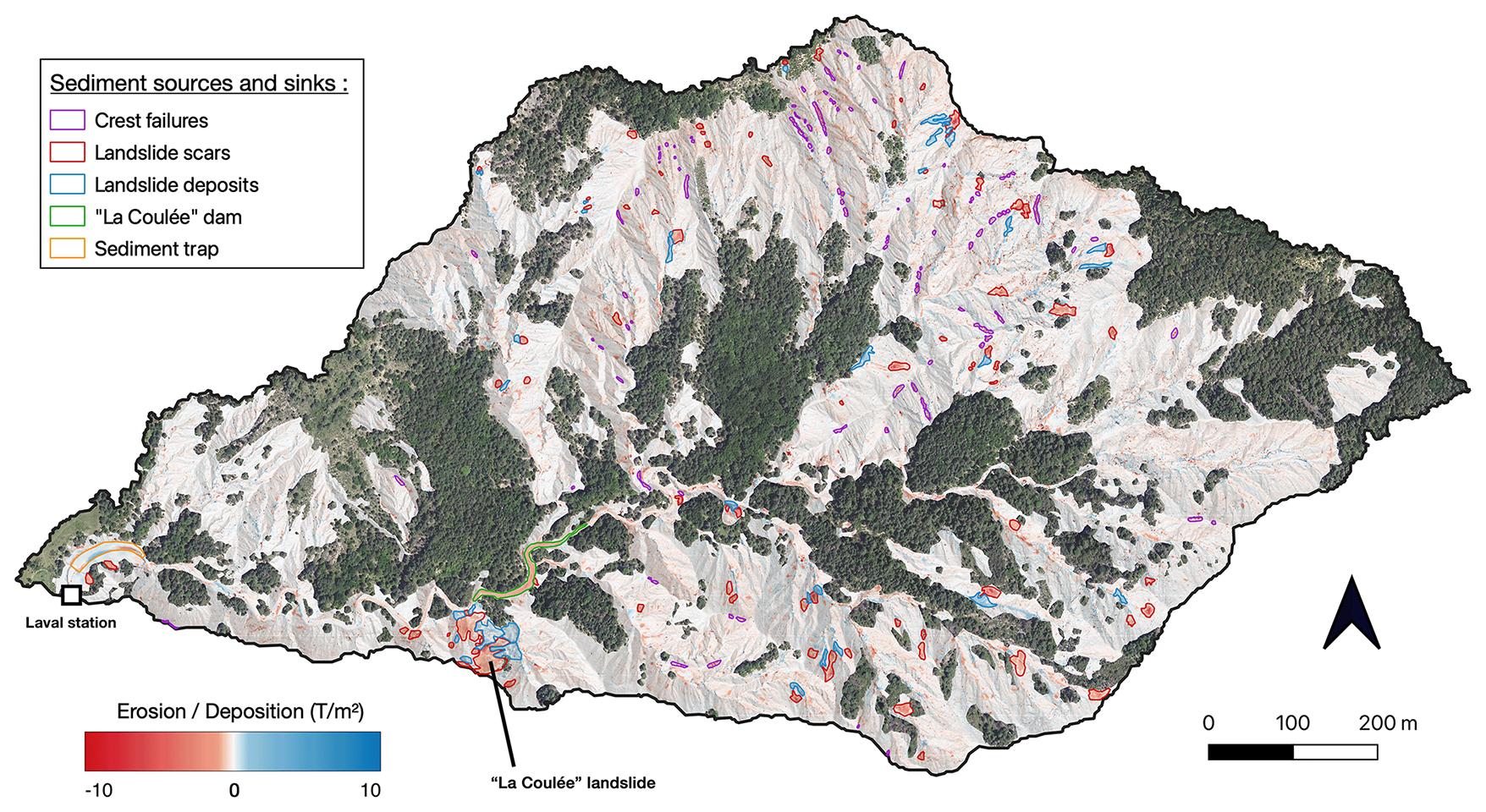
Figure 5 Map of local erosion (in red) and deposition (in blue) over the Laval catchment (French Alps) between the 2015 and 2021 LiDAR surveys over the Laval catchment (French Alps). Vegetated areas have been masked using an orthophotography (IGN, 2021). An inventory of the sediment sources and sinks has been overlaid.

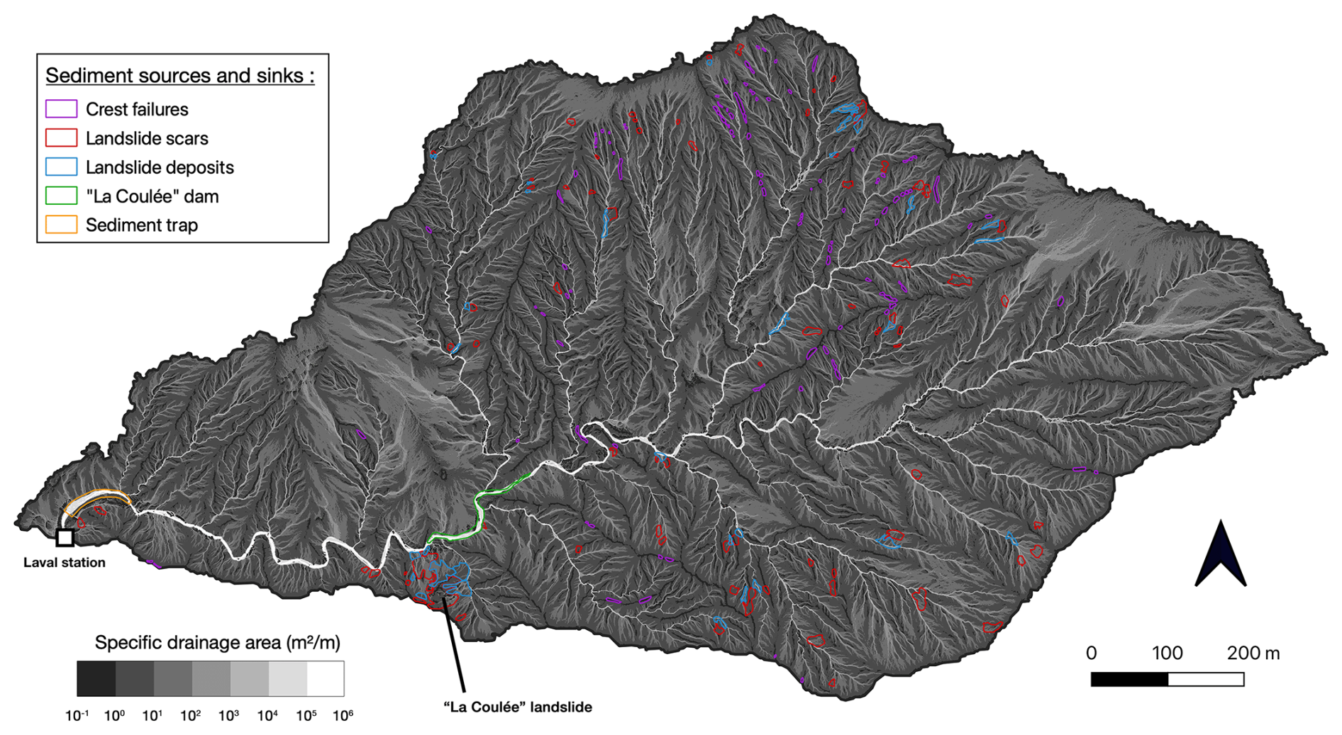
Figure 6 Map of the specific drainage areas, binned in logarithmic intervals and computed with the Graphflood algorithm (Gailleton et al., 2024), assuming a runoff rate of 50 mm h⁻¹ and based on a 50 cm-resolution DTM derived from the 2015 LiDAR survey. An inventory of the sediment sources and sinks has been overlaid.

4.2 Contributions to the sediment export

Calculating the total LiDAR sediment budget at catchment scale ∑_xyδM_xy, excluding vegetated areas, yields an export estimate of 60 ± 20 kT over the 6-year sequence. This uncertainty range reflects the upper- and lower-bound sediment density profiles used in Sect. 3.2, while volume-related uncertainties are minimal, amounting to no more than one kilotonne. Using the central density profile, the estimated export corresponds to 67 % of the sediment export recorded at the outlet, which is approximately 89 ± 30 kT. As the two sediment budget values are expected to match, the 23 % discrepancy is attributed to measurement uncertainties in the station records, simplified bulk density modelling and, to a lesser extent, limitations of the LiDAR processing workflow, as discussed further in Sect. 5.4.

Sediments produced by landslides account for a significant proportion (14 %) of the outlet export, but occupy less than 1 % (0.8 ha) of the catchment surface area. However, as 29 % of the landslide material remains on the slopes, on average, this proportion falls to 10 % during the sequence. Similarly, the erosion observed on ridge tops accounts for 4 % of the export and covers only 0.2 ha (four times less than landslides). These estimates may be underestimated as there is a 23 % discrepancy between the sediment budget estimated from records and that estimated from the LiDAR surveys.

Figure 5 shows that significant erosive activity occurred in association with the “La Coulée” landslide that took place on the left bank of the main channel in December 1998. This structural landslide mobilised 4500–5600 m³ of compact marl (Fressard and Maquaire, 2009), corresponding to 12 to 15 kT. It struck the opposite slope and temporarily obstructed the Laval main channel, which gradually evacuated the materials (Malet, 2003; Mathys, 2006). This activity continues as the landslide has generated an additional 2.2 kT of sediment between our two surveys. Of this, 0.7 kT did not reach the main channel and remained on its slopes, as can be seen in Fig. 5.

The timescale of the multi-temporal LiDAR analysis is such that Fig. 5 integrates several of the seasonal variations observed in the main channels, as documented by Bechet et al. (2016), Jantzi et al. (2017) and Liébault et al. (2022), which complicates the interpretation. Nevertheless, the significant erosion signal ($-\mathrm{1.7}\pm \mathrm{0.2}$ kT) detected in the channel directly upstream of the landslide indicates that the obstruction is still disrupting sediment transport within the basin. This obstacle appears to have created a temporary reservoir, which can be filled under a transport-limited erosion regime or emptied under a supply-limited regime.

4.3 Spatial distribution of changes within the drainage network

Figure 7a shows the distribution of local mass variations due to erosion or deposition as a function of the corresponding specific drainage area. This indicates the sources and sinks that were previously identified in Figs. 5 and 6. A second scale illustrates the correspondence between the specific drainage area and the upslope contributing area (Fig. C1a).

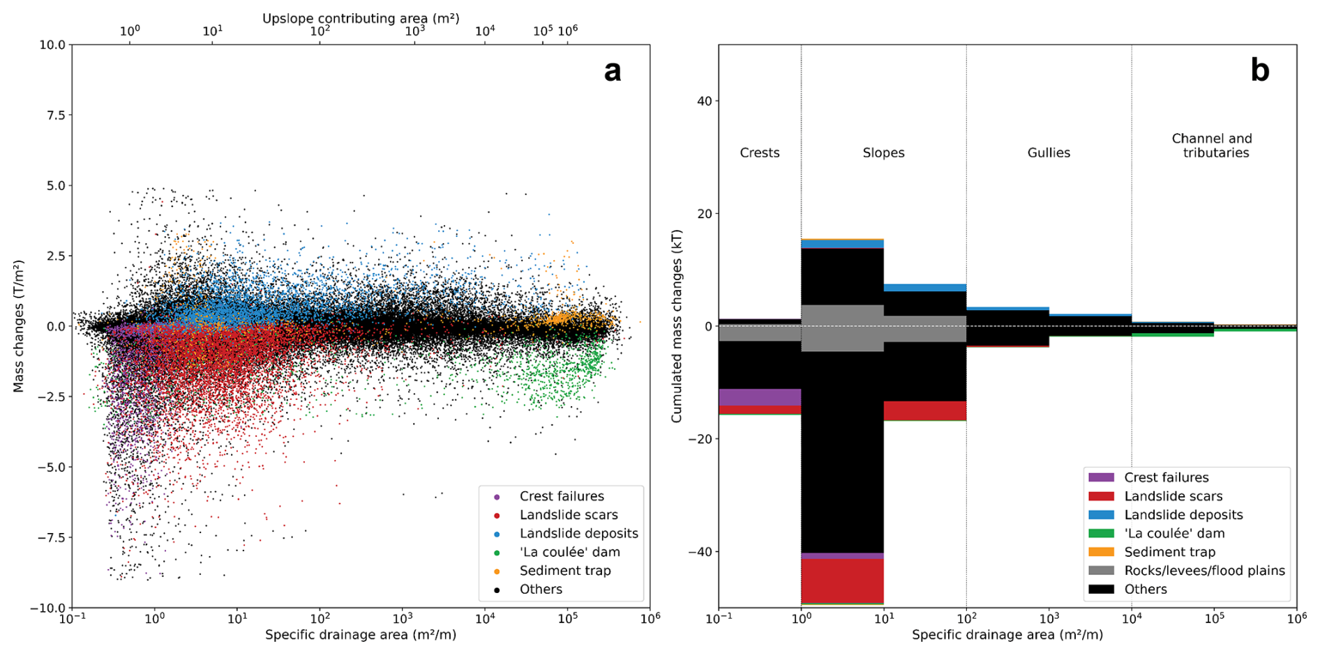
Figure 7 (a) Distribution of local mass variations as a function of the associated specific drainage area (left plot) at any point in the denuded regions, (b) cumulated in each log interval of specific drainage area. The sediment sources and sinks identified above are shown in the same colours. Contributions from levees, large boulders and floodplains with a small drainage area that belong to the drainage network area are also shown in gray.

As mentioned in Sect. 4.1, the majority of points correspond to mass changes between −1 and +1 T m⁻² and are distributed accross all drainage areas. However, nearly 50 % of the sediment budget originates from outside this range. Points with higher deposition are mainly concentrated in the specific drainage areas between 10⁰ and 10¹ m² m⁻¹ and to a lesser extent, between 10¹ and 10⁴ m² m⁻¹, mostly corresponding to landslide deposits. Points of higher erosion are mainly concentrated in specific drainage areas below 10² and above 10⁴ m² m⁻¹, corresponding respectively to crest erosion, landslide erosion and main channel drainage.

Examining the sums of positive (deposition) and negative (erosion) cumulative mass changes for each specific drainage area logarithmic interval makes it possible to determine their contribution to the sediment budget, as well as that of the labelled sediment sources and sinks within them (Fig. 7b). As some signals from low drainage areas actually correspond to levees, large boulders, floodplains and terraces above the flood level of the main channel and its tributaries, we define a 1 m-buffer around gullies and channels with a specific drainage density above 10³ m² m⁻¹ and a 2 m-buffer above 10⁴ m² m⁻¹. This creates another class in Fig. 7b. Figures 6 and 7b show that, by reassigning this contribution to the channels, specific drainage areas feed into each other from ridges to slopes and finally into the drainage network. Taking this adjustment into account, we therefore assume that the log intervals of specific drainage area may actually reflect geomorphological units that are susceptible to produce and transport sediments with different dynamics:

• The crests typically have submetric specific drainage areas, i.e., upslope contributing areas ranging from 0 to approximately $\mathrm{1}/\mathrm{3}$ m². For these drainage ranges, 17 % of the sediment budget corresponds to rocks and levees in the channels, 19 % to the previously identified crest failures and around 9 % to landslide scars. The latter two together occupy around 6 % of the compartment's surface area. It can be assumed that raindrop splash erosion (Wischmeier and Smith, 1958; Legout et al., 2005; Leguédois et al., 2005) contributes to diffuse erosion in this compartment (Marsico et al., 2021). As expected, there is almost no accumulation, with the sediment budget totalling 12 kT, i.e., 20 % of the overall export for less than 7 % of the denuded area.

• The slopes are defined by the following two log intervals of specific drainage area, ranging up to 100 m². Over these log intervals, crest failures are negligible but landslide scars account for 16 % and 20 % of the sediment budget respectively, while deposits account for 9 % and 17 % (2 %–3 % of the corresponding surface areas). Most of the signals for deposition and erosion are not classified and probably correspond to diffuse processes such as erosion by sheet washing, soil creep or erosion/filling or small rills on slopes. Once again, up to 17 % of the cumulative mass changes over these log intervals correspond to levees and floodplains belonging to the drainage network. Excluding these contributions, the slope compartment accounts for 69 % of the overall sediment budget, while occupying 79 % of the denuded areas.

• The remaining four log intervals describe the drainage network itself, with gullies of up to 10⁴ m² (1 ha) for the main channel and tributaries. This is consistent with the assumptions made in Bechet et al. (2016) and Nadal-Romero et al. (2011). Compared to the previous compartment, the signal corresponding to the drainage network is small, even in the main channel, where, we identified in Sect. 4.2 a natural dam upstream of the “La Coulée” landslide (1.7 kT), or taking into account the levees, floodplains and terraces (−4 kT). A signal up to 2.4 kT could have been observed coming from the 1400 m³ sediment trap, but this is not the case as it appears at the same filing level between the two campaigns (Fig. 5).

5 Discussion

5.1 Active mass wasting areas

Our study emphasises the significance of landslide scars and crest failures as erosional hotspots. As estimated in Sect. 4.2, these features contribute around 15 % of the basin's sediment budget, despite affecting only 1 % of the bare soils. More specifically, they make a significant contribution to the specific drainage areas ranging from metres to tens of metres, accounting for half of the strongest signals exceeding 1 T m⁻².

As our study covers a period of 6 years, it is reasonable to assume that these active unstable zones are not necessarily the result of a single slope failure. Instead they may have experienced a succession of smaller movements to clear the debris accumulated downstream due to incision or headwater recession (Nadal-Romero and García-Ruiz, 2018). This is particularly evident in the case of the “La Coulée” landslide, which continues to experience significant erosive activity two decades after being triggered. Consequently, and despite the size of these active zones, we believe that our results may be consistent with those of Wijdenes and Ergenzinger (1998) and Yamakoshi et al. (2009) on miniature debris flows (MDF). However, this remains to be examined in detail, as these authors claim that MDFs play a crucial role in the transport of coarse sediments, contributing between 5 % and 36 % of the total export of the neighbouring Roubine basin.

Finally, our study shows that, on average, 29 % of landslide deposits remain on the slopes over the studied period. Supplementing the time series with other high spatial resolution campaigns, as well as specific event-scale surveys, would enable the drainage of these materials to be monitored, the geomorphological processes involved to be characterised and, the evolution of these active areas to be described more generally. While Sect. 3.3 showed that this 6-year sequence provides a representative record of sediment export, incorporating additional campaigns would further consolidate estimates of sediment export contributions and help determine whether these are characteristic of these badlands.

5.2 Sediment production of the main geomorphological units

In Sect. 4.3, it was observed that the specific drainage area defines hydrologically ordered geomorphological units. Following the adaptation of the landscape partitioning method developed by Montgomery and Foufoula-Georgiou (1993) as proposed by Bernard et al. (2022), which distinguishes convex hillslopes, unchanneled valleys, and the fluvial domain based on the inflection points of the hydraulic slope–specific drainage area relationship in a log–log diagram, Fig. C1b reveals a relatively good correspondence with the crest, slope, and drainage network components (including gullies, channels, and tributaries) that we define here. However, it should be noted that transitions between hydro-geomorphological domains are not clear-cut, even with this convexity-based partitioning method. Furthermore, as demonstrated in calanchi badlands by Vergari et al. (2019), this functional relationship is insufficient to accurately separate geomorphological process domains in such environments, since these processes can operate and interact within the same drainage areas.

Sediment budgets can still be calculated for each compartment, taking into account that they are interconnected and may be subject to transient sediment deposition and drainage, as sediment tends to move in pulses across the landscape (Puigdefabregas et al., 1999). Some areas with low specific drainage correspond to features such as levees, floodplains or large boulders located in or near the main channel. These areas are therefore reassigned to the drainage network compartment, as detailed in Sect. 4.3.

In order to derive the corresponding production rates, the contributions due to remobilisation must be excluded. To achieve this, we consider two boundary cases for each compartment, corresponding to the transition from a transport-limited regime to a supply-limited regime, or vice versa. The first campaign may occur at a time when erosion is transport-limited, resulting in the accumulation of at most the total upstream production, in a given compartment. These deposits may be drained between the two campaigns, with the second campaign occurring when erosion is supply-limited. Therefore, the sediment budget in this compartment may overestimate the amount of sediment produced inside by up to the total upstream production. Subtracting the total upstream production from the sediment budget would then provide a lower-bound estimate of the sediment production in the given compartment. Conversely, the second campaign may have occurred when the given compartment was accumulating material produced upstream under transport-limited conditions, whereas the first campaign occurred in a supply-limited regime. Again, these deposits may represent at most all of the material produced upstream, meaning that when erosion rates are derived from a multi-temporal analysis, the sediment production of the compartment may be underestimated by as much. Adding the upstream production would then provide an upper-bound estimate of the sediment production.

Figure 8 shows a conceptual model of the various geomorphological units found in a badland catchment area. Insets (a) and (b) show two examples of mass movements, with the source areas located in the crest and slope units, respectively. An initial LiDAR survey conducted at this stage would capture a transport-limited erosion regime in the slope compartment, as the landslide deposits remain stored on the slopes. A later survey, conducted when the slope compartment is under a supply-limited regime, might measure the remobilisation of these deposits, resulting in a strong erosion signal recorded in both areas. For inset (b), this signal would accurately reflect sediment production in the slope compartment. However, the calculation framework presented here ensures that the erosion signal observed in inset (a) may instead reflect production from the crests. Conversely, if the landslides occurred between the LiDAR surveys and the conceptual model represents the subsequent topography, a change map similar to Fig. 5 would show strong signals originating from the crests in inset (a), which would be accurately reflected in the sediment production of this compartment by the presented method. However, sediment production from the slope compartment would be underestimated due to the presence of deposits. Nevertheless, the proposed method provides a lower-bound estimate for this compartment. Sediment production associated with the landslide in inset (b) would only be accounted for once deposits have been removed from the slope compartment.

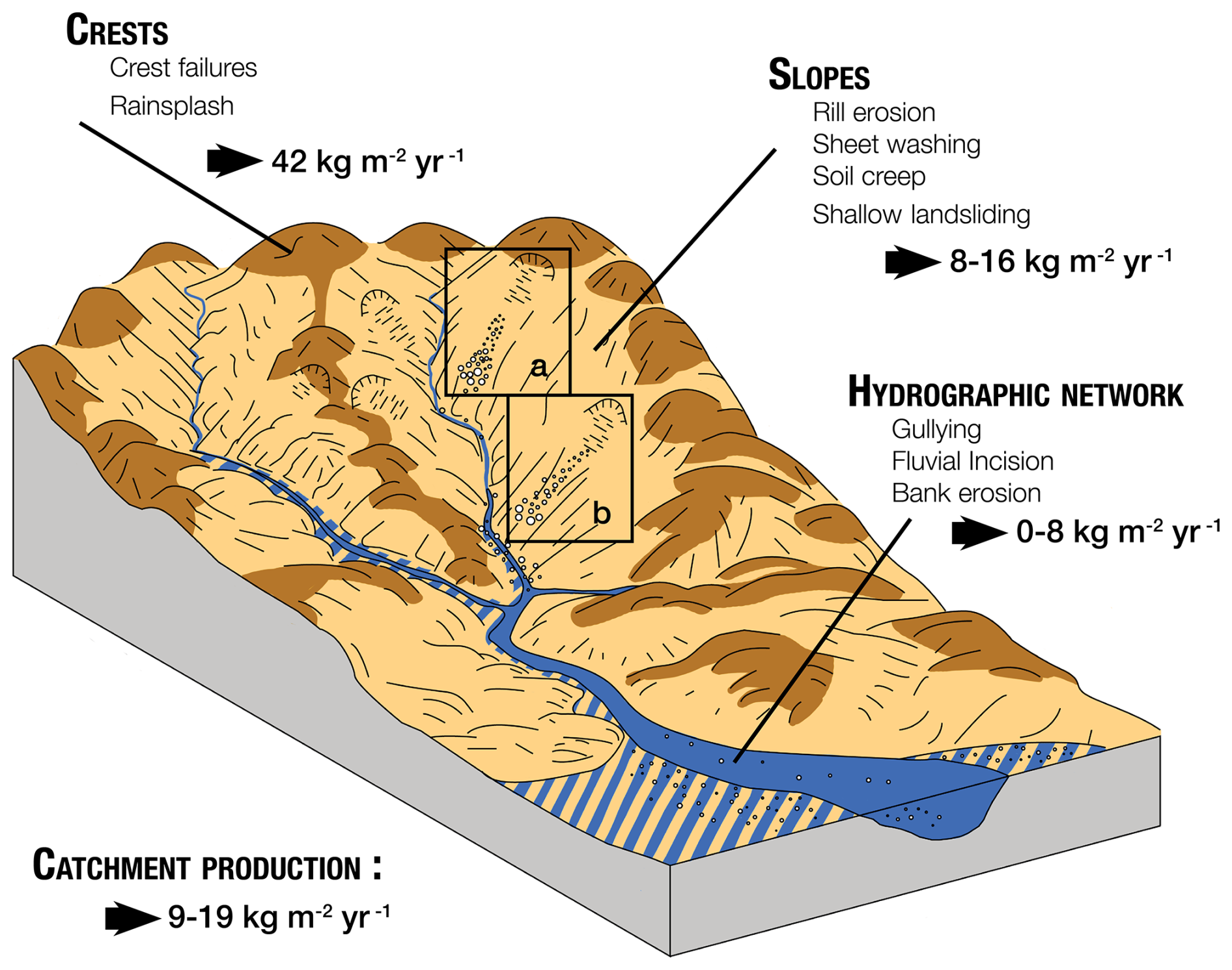
Figure 8 Conceptual model of sediment production across the main geomorphological units of a badland catchment. Levees, large boulders and floodplains with a small drainage area that belong to the drainage network area are also represented with hatching. Boxes (a) and (b) depict two mass movements, with the source areas located in the crest and slope units, respectively, and downslope deposits. The figure also illustrates some of the processes that are potentially responsible for primary sediment production. Schematic adapted from Stock and Dietrich (2006).

In our case study, the production rate for crests not fed from upstream is simply the ratio of the sediment budget for the compartment to its corresponding area. We obtained a value of 42 kg m⁻² yr⁻¹. This is twice the 21±7 kg m⁻² yr⁻¹ export measured at the outlet. For the slopes, the previous approach gives a production rate ranging from 16 to 8 kg m⁻² yr⁻¹ with an indicative value of −12 kg m⁻² yr⁻¹, which is already lower than the average value obtained from outlet export, but in line with the 14±5 kg m⁻² yr⁻¹ obtained with LiDAR sediment budget. As the late spring rainfall events of 2021 (see Fig. 2) appear to have drained the “La Coulée” natural dam, as can be seen in Fig. 5, we are likely closer to the former scenario in the drainage network. This would mean a transition from a transport-limited regime during the first campaign in early April 2015 and a supply-limited regime during the second campaign in June 2021. This suggests that sediment production in this compartment is between 0 and 10 kg m⁻² yr⁻¹, or even between 0 and 8 kg m⁻² yr⁻¹ under the assumption that the natural dam and the sediment trap solely store upstream materials and do not contribute to sediment production. However, these values could be underestimated, given the 23 % discrepancy in the sediment budget between the LiDAR survey estimation and the measured export. These sediment production estimates from each geomorphological compartment, as well as the geomorphological processes that can potentially be responsible for these primary sediment productions, are summarized in the conceptual model illustrated in Fig. 8.

5.3 Insights across spatial and temporal scales

A characteristic of badlands is the conjunction of sparse vegetation, steep slopes of over 45°, and impermeable marl bedrock beneath the weathered layer. This favours the initiation of Hortonian runoff between the gullies, which effectively washes away the altered material produced on the bare slopes in winter (Descroix and Olivry, 2002; Descroix and Mathys, 2003). In line with the data analysed by Nadal-Romero et al. (2011) or Marsico et al. (2021), and in contrast to other Mediterranean environments (De Vente and Poesen, 2005; De Vente et al., 2007), our study shows that the areas producing the most sediment in badlands are those with the lowest drainage area and the steepest slopes. In this way, we can measure 75 % of the export for specific drainage areas smaller than 10 m² m⁻¹ (approximately two-third of bare areas) and 20 % of the export solely for submetric specific drainage areas (less than 7 % of the bare areas). In accordance with the corrigendum (Nadal-Romero et al., 2014) to the study of Nadal-Romero et al. (2011), Fig. 7 shows lower production below 1 m² of upslope contributing area (smaller than the sampling scale) where the slope becomes convex, no longer concentrates runoff, and is probably characterised only by “splash erosion”. However, as soon as this limit is exceeded, the erosion processes driven by the steepness of the slope are so efficient that the crests compartment defined above has a production rate twice as high as that of the rest of the slopes. As confirmed in our study, the predominant influence of slope accounts for the notable agreement between our erosion map (Fig. 5) and that produced by (Saez et al., 2011), who calibrated a slope–erosion relationship using dendrochronological data.

Another important driver of erosion is the nature of the substrate, as emphasised by Descroix and Mathys (2003). Although the lithology is relatively homogeneous in the Draix badlands, leading these authors to propose parallel erosion and constant slope angles, our study challenges this assumption at the considered timescale. Furthermore, heterogeneity in weathering depth across interfluves, slopes and thalwegs has been reported by Maquaire et al. (2002), Rovéra and Robert (2006) and Ariagno et al. (2023), with deeper weathering profiles on ridge tops and shallower ones in thalwegs. This suggests that, from an in situ sediment production perspective, thalwegs operate under a supply-limited regime. In contrast, ridge tops, despite experiencing higher erosion rates, do not exhibit such limitations. This indicates highly effective winter weathering processes, likely sustained by the removal of weathered material in summer, which continuously exposes fresh substrate. This dynamic may also be influenced by the presence of more resistant calcareous layers that are progressively being exhumed by erosion and which have been observed in thalwegs. This has previously been noted for the Blue Marls by Descroix and Mathys (2003). It is worth noting that such heterogeneity in weathering profiles across ridge tops, slopes and thalwegs may lead to misestimation of production rates in these units. This issue is discussed further in Sect. 5.1. Given the feedback loops between topography and erosion, it would also be valuable to consolidate our findings on the distinct evolution of geomorphological units over time through long-term monitoring.

The timescale of the study determines the processes to which a multi-temporal analysis can be sensitive. Accumulating data over years makes gradual erosion easier to detect and reliably quantify on the top of slopes that are unlikely to temporarily store sediment, particularly where the terrain is very steep. This also enables mean production rates to be estimated that compensate for inter-annual variability and provide a representative description of the behaviour of the basin over these timescales. Conversely, adapting this method to characterise sediment connectivity in the drainage network requires finer temporal resolution to capture the seasonal alternation between transport-limited erosion in winter and supply-limited erosion in summer (Bechet et al., 2016; Ariagno et al., 2022). Alongside finer spatial resolution, we should be able to link large-scale mass movements to climatic forcing. This could improve the modelling of sediment transport during floods and provide insight into hysteresis loops, particularly clockwise loops observed at hydro-sedimentary stations (Roque-Bernard et al., 2023), which we suspect may be related to debris flow inputs from slopes or gullies.

5.4 Methodological constraints

To our knowledge, this is the first study to combine sediment export measurements at the outlet (89 ± 30 kT) and maps of mass movements over bare slopes (60 ± 20 kT) to perform a catchment-scale mass balance and determine its sediment budget. The performance of this method depends on:

• The quality of the LiDAR time series (point cloud density and accuracy) and its co-registration, assessed over stable zones. The sensitivity of our global sediment budget to a z-shift is around 10 kT cm⁻¹, while our uncertainty on z is estimated to be in the millimetre to centimetre range at most (Fig. D1).

• Reconstitution of local variations in volume. The associated uncertainties essentially result from the choice of grid cell size, plus or minus 8 kT, depending on whether a size of 0.5 m × 0.5 m or 2 m × 2 m is chosen. The 1 m value limits the number of empty cells for which the value must be interpolated. The other uncertainties propagated in the processing chain amount to a few hundred tonnes at most. Additionally, rainwater infiltration can cause regolith to swell or shrink by a few millimetres, as described in (Bechet et al., 2015). This could result in a weak signal that is not characterised here and does not correspond to erosion.

• The design of a bulk density model to convert local volume changes during the sequence into local mass changes. This is the most difficult variable to constrain, since the spatial and temporal variability of weathering and deposition profiles can significantly alter our estimates of displaced or accumulated mass (Ariagno et al., 2023; Maquaire et al., 2002; Travelletti et al., 2012). The density ranges defined in Sect. 3.2 provide sediment budget uncertainty estimates of ± 20 kT, i.e., 7 kT per 0.1 g cm⁻¹ systematic shift in the density profile shown in Fig. 4. Future work could focus on developing bulk density profiles specific to different geomorphological processes or units, as some authors have identified deeper weathering on interfluves than on thalwegs (Maquaire et al., 2002; Rovéra and Robert, 2006; Ariagno et al., 2023). This approach would be particularly relevant, given that neglecting this aspect leads to an overestimation of production on crests and an underestimation of production in thalwegs.

• Measurement uncertainties at the outlet, both in terms of suspension and deposition in the sediment trap. They mainly reflect the difficulty of calibrating turbidity measurements to estimate suspended matter at low concentrations, as detailed in Table B1 and the data paper by Klotz et al. (2023). These uncertainties range within ±30 kT over the period.

Our work has been carried out on bare badland formations, excluding vegetated areas, as these are likely to have a very different weathering profile compared to that proposed by the density model. In any case, while they may be sites of deposition or transport, material flow is expected to be low due to soil fixation by roots (Rey, 2003; Burylo et al., 2011, 2012; Carriere et al., 2020; Bunel et al., 2025). Additionally, the density of LiDAR points classified as “ground” is lower under vegetation, which makes it more challenging to reconstruct the topography of surfaces that may be littered with plant leaves or shrubs.

Finally, this study carries out an inventory of sediment sources and sinks manually using a GIS tool, which has limitations in terms of contour delineation and detection thresholds (Guzzetti et al., 2012). An alternative approach, which is also subject to merging and underdetection problems (Li et al., 2014; Marc and Hovius, 2015; Tanyaş et al., 2019), could be based on supervised or unsupervised clustering (Borghuis et al., 2007; Parker et al., 2011). This would be similar to the methods used for landslide detection, which use pixel-based approaches (Mondini et al., 2011; Lu et al., 2019), object-oriented approaches (Stumpf and Kerle, 2011; Keyport et al., 2018) or deep learning approaches (Ghorbanzadeh et al., 2019; Prakash et al., 2020). A more detailed characterisation of the geomorphological processes at play could be achieved by analysing hydro-geomorphological metrics in more detail, using approaches such as the MaGPiE algorithm, which was developed specifically for badlands (Llena et al., 2020a, b).

5.5 Opportunities in a changing climate

Mediterranean environments are among the regions most affected by climate change. They are projected to experience a significant decrease in precipitation (except in winter in the southern French Alps), as well as an increase in temperature and in the frequency of paroxysmal events (Giorgi and Lionello, 2008). Therefore, it is crucial to assess the impact of these changes on the future evolution of critical zone processes, particularly in vulnerable environments such as badlands, which contribute significantly to sediment export (Copard et al., 2018). It is unclear how their erosive dynamics, which are closely linked to vegetation dynamics (Gallart et al., 2013), will evolve in the context of a decrease in winter weathering caused by cryoclastic forcing (Ariagno et al., 2022), and a decrease in summer precipitation competing with an increase in the number and intensity of summer storms that trigger landslides (Gariano and Guzzetti, 2016; Turkington et al., 2016; Hirschberg et al., 2021; Nadal‐Romero et al., 2022).

However, the widespread availability of high-resolution data is paving the way for the development of geomorphological analysis tools that can quantify and spatialize sediment sources and sinks. The methodology developed in this study offers new prospects for analysing erosion and sediment transport at different scales within a catchment. It complements existing observation methods and could help to improve the accuracy of hydro-sedimentary transport models, which already simulate runoff response to precipitation forcing in these catchments accurately, but have limited predictive ability for sediment fluxes (Lukey et al., 2000; Mathys et al., 2003; Carriere et al., 2020; Bunel et al., 2025).

6 Conclusion

We analysed erosion in a small badland catchment by combining a 6-year analysis of LiDAR data with a material bulk density model. This enabled us to calculate a total mass loss of 60 ± 20 kT, equivalent to an annual erosion rate of 200 T ha⁻¹ yr⁻¹ in denuded areas. This represents a 23 % discrepancy compared to the export measured at the long-term outlet hydro-sedimentary station, which is likely due to measurement uncertainties and density modelling. Our findings indicate that landslides and ridge failures are significant contributors to the total sediment export (15 % of the total export for 1 % of the total surface area). Furthermore, low specific drainage areas are the most productive (20 % of the total erosion for 7 % of the total surface area), while the channel network appears to be primarily driven by the remobilisation of sediments produced upstream. Our method appears to be a promising approach for assessing sediment transport in badlands in a changing climate.

Appendix A: Rasterization of local volume changes from cloud-to-cloud distances

The M3C2 algorithm (Lague et al., 2013) presented in Sect. 3.1.2 is used to evaluate the local distances between two point clouds. A Geotiff raster with a resolution of 1 m² pixels is constructed using 5 scalar fields:

• the average distance between clouds in each cell h_⟂;

• the corresponding uncertainty value dh_⟂;

• the cell point population p;

• the mean point height z;

• the uncertainty on this height value dz.

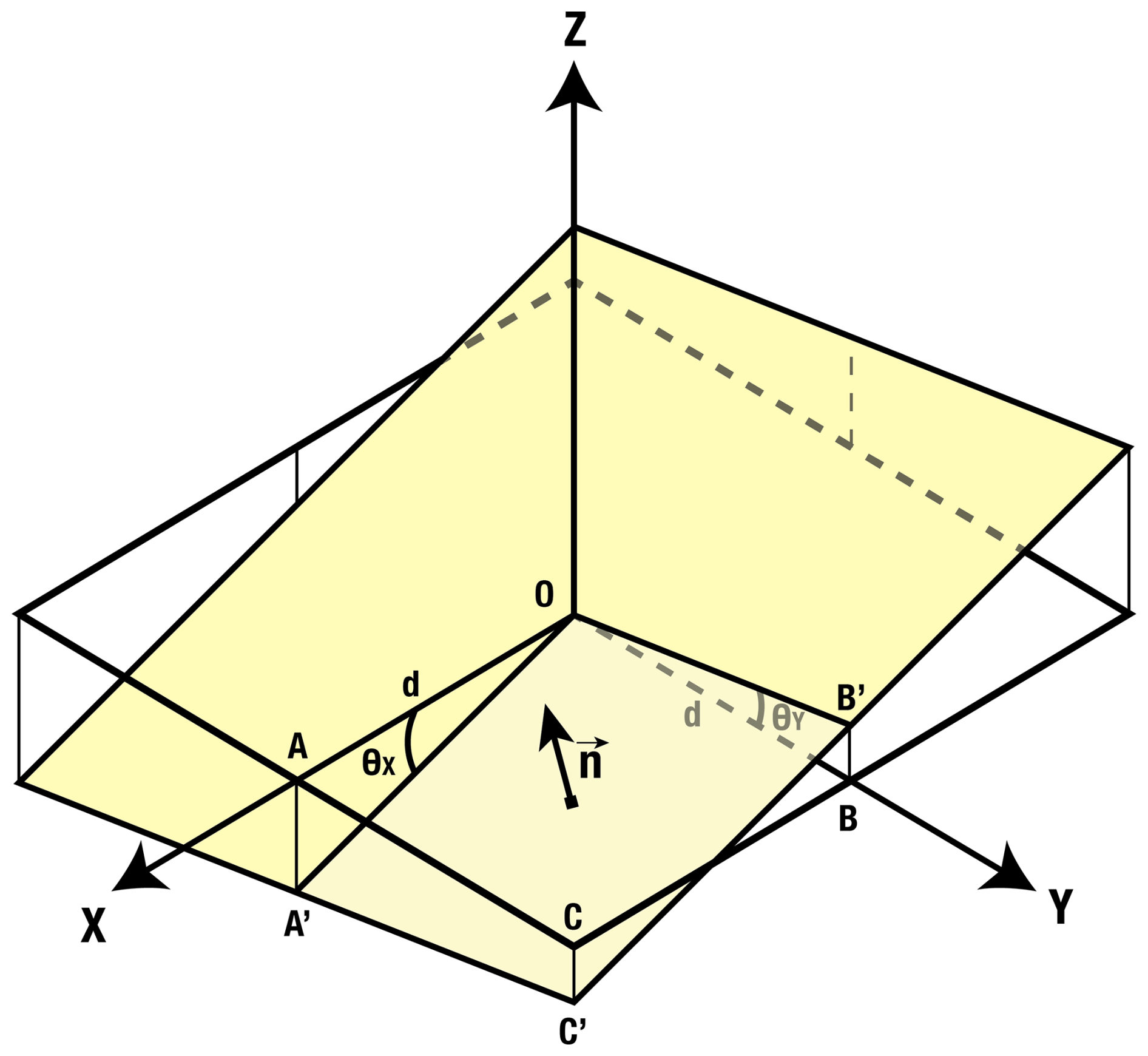
Figure A1 Geometry used to calculate the area of oriented facets describing local surface depletion or accumulation.

The surface model is then used to derive the gradient components in the X and Y directions of the grid. The population of each cell is information that can be used to filter cells if, for example, an outlier value is suspected. To calculate the area intercepted by each mesh in the grid, the grid is locally modelled by a plane whose inclination (θ_x,θ_y) is given by the components of the gradient in the X and Y directions. The same assumptions are made as for the shallow water equations (see Sect. 4.3), namely that the choice of grid size causes the length scale for the curvature of the topography to be much larger than the length scale at which normal variations h_⟂ are considered. Considering one quadrant of each facet and the plane equation:

$$\begin{array}{c}{\displaystyle }\begin{array}{rl}& \left\{\begin{array}{l}{\mathbf{OA}}^{\prime }=(d,\mathrm{0},d\times \tan {\mathit{\theta }}_x)\\ {\mathbf{OB}}^{\prime }=(\mathrm{0},d,d\times \tan {\mathit{\theta }}_y)\end{array}\right.\\ & \Rightarrow {\mathbf{A}}^{\prime }{\mathbf{B}}^{\prime }=d\times (-\mathrm{1},\mathrm{1},\tan {\mathit{\theta }}_y-\tan {\mathit{\theta }}_x)\end{array}\\ {\displaystyle }\exists \mathit{n}\mathrm{|}{\mathbf{O}}^{\prime },{\mathbf{A}}^{\prime },{\mathbf{B}}^{\prime },{\mathbf{C}}^{\prime }\text{ satisfy }{n}_{x}x+n_{y}y+n_{z}z=\mathrm{0}\\ {\displaystyle }\begin{array}{rl}& \Rightarrow x\tan {\mathit{\theta }}_x+y\tan {\mathit{\theta }}_y-z=\mathrm{0}\\ & \Rightarrow {\mathbf{OC}}^{\prime }=d\times (\mathrm{1},\mathrm{1},\tan {\mathit{\theta }}_x+\tan {\mathit{\theta }}_y)\end{array}\end{array}$$

This gives the area ${\mathcal{S}}_{O{A}^{\prime }{B}^{\prime }{C}^{\prime }}$ of each facet quadrant as half the product of the diagonals:

$$\begin{array}{rl}{\mathcal{S}}_{O{A}^{\prime }{B}^{\prime }{C}^{\prime }}=& {\displaystyle \frac{d^{\mathrm{2}}}{\mathrm{2}}}\sqrt{(\mathrm{2}+(\tan {\mathit{\theta }}_x+\tan {\mathit{\theta }}_y{)}^{\mathrm{2}}}\\ & \sqrt{(\mathrm{2}+(\tan {\mathit{\theta }}_x-\tan {\mathit{\theta }}_y{)}^{\mathrm{2}}}\end{array}$$

Voxels can be formed in each cell: the third dimension is given by the M3C2 distance and their volume corresponds to the local erosion/deposition value:

$${\mathcal{V}}_{\mathrm{voxel}}=\mathrm{4}\times {\mathcal{S}}_{O{A}^{\prime }{B}^{\prime }{C}^{\prime }}\times h_{⟂}$$

Note that the sign of 𝒱_voxel is given by the sign convention for h_⟂, which allows us to distinguish erosion values from deposition values. Uncertainties can also be applied to the volume calculation:

$$\mathrm{d}\mathcal{V}=h_{⟂}\left({\partial }_{{\mathit{\theta }}_x}\mathcal{S}\mathrm{d}{\mathit{\theta }}_x+{\partial }_{{\mathit{\theta }}_y}\mathcal{S}\mathrm{d}{\mathit{\theta }}_y\right)+S_{O{A}^{\prime }{B}^{\prime }{C}^{\prime }}\mathrm{d}{h}_{⟂}$$

where dh_⟂ is one of the scalar fields contained in the Geotiff frame, as well as dz_x+1, $\mathrm{d}{z}_{x-\mathrm{1}}\mathrm{d}{z}_{y-\mathrm{1}}$, and dz_y+1, which allows dθ_x and dθ_y to be calculated. The barycentre of each cell itself has a positional uncertainty in the plane which is also taken into account by the cell population p.

Appendix B: Focus on uncertainties in hydro-sedimentary chronicle data

In Sect. 3.1 we present the cumulative sediment export of suspended M_susp and deposited M_dep. sediments at the outlet of the watershed calculated with:

$$\left\{\begin{array}{l}{M}_{\mathrm{susp}.}=\sum _t{C}_{\mathrm{susp}.}\left(t\right)\times Q\left(t\right)\\ M_{\mathrm{dep}.}=\sum _t{V}_{\mathrm{dep}.}\left(t\right)\times {\mathit{\rho }}_{\mathrm{trap}}\end{array}\right.$$

where C_susp. and Q are the concentration of suspended sediments (kg m⁻³) and water discharge (m³ s⁻¹), respectively, and V_dep. and ρ_trap correspond to the deposited volume in the sediment trap (m³) and its associated dry bulk density (kg m⁻³). The value used for dry bulk density is ρ_trap=1700 kg m⁻³.

In the data paper of Klotz et al. (2023), the characterisation of measurement uncertainties is presented in the form of quality codes assigned during the expertise of the data (Table B1). When no quality codes are attributed we assume an intermediate quality, as at that time poor quality data where classified as missing data. There are no data entries flagged as “low quality” in these datasets, although this may occur for rainfall data for instance. Without further assumptions on their distribution, they are considered as expanded uncertainties propagated by the following equations:

$$\left\{\begin{array}{l}\mathrm{\Delta }\left(\sum _i{X}_i\right)=\sum _i\mathrm{\Delta }\left(X_i\right)\\ \frac{\mathrm{\Delta }\left({\prod }_i{X}_i\right)}{{\prod }_i{X}_i}=\sum _i\frac{\mathrm{\Delta }\left(X_i\right)}{X_i}\end{array}\right.$$

Table B1 Correlation between hydro-sedimentary data quality codes and their corresponding uncertainties, adapted from Klotz et al. (2023).

Appendix C

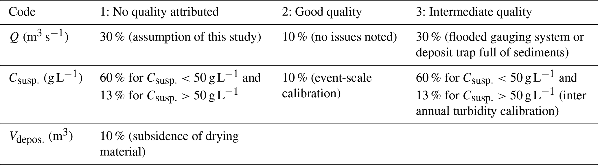
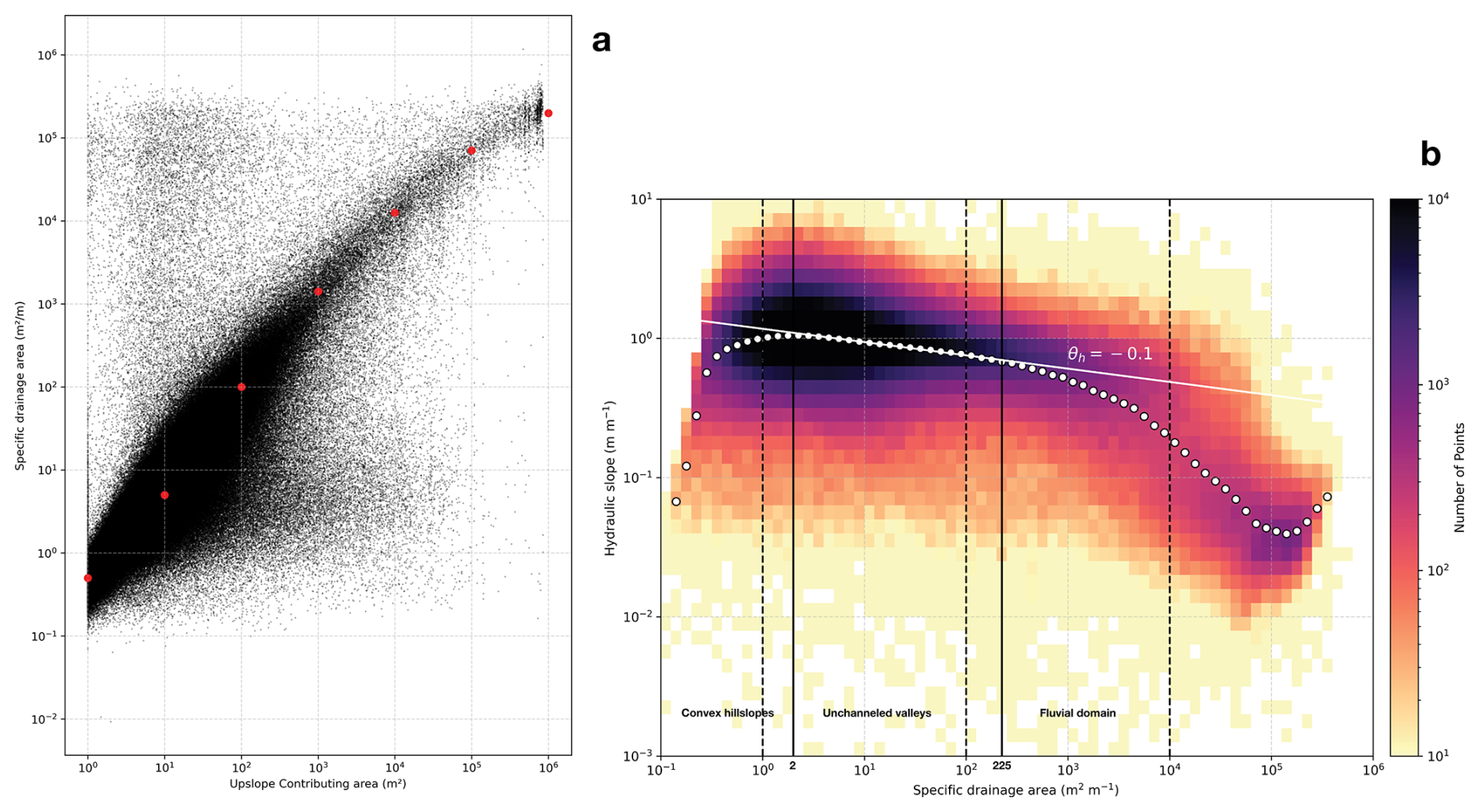
Figure C1 (a) Specific drainage area (m² m⁻¹) against upslope contributing area (m²) for a runoff rate of 50 mm h⁻¹. (b) 2D histogram showing hydraulic slope as a function of specific drainage area. White dots indicate average values within logarithmic bins of specific drainage area. Solid vertical lines delineate geomorphological domains with the inflection point method, while the dashed vertical line marks this study's definition of the crest, slope, and drainage network units.

Appendix D

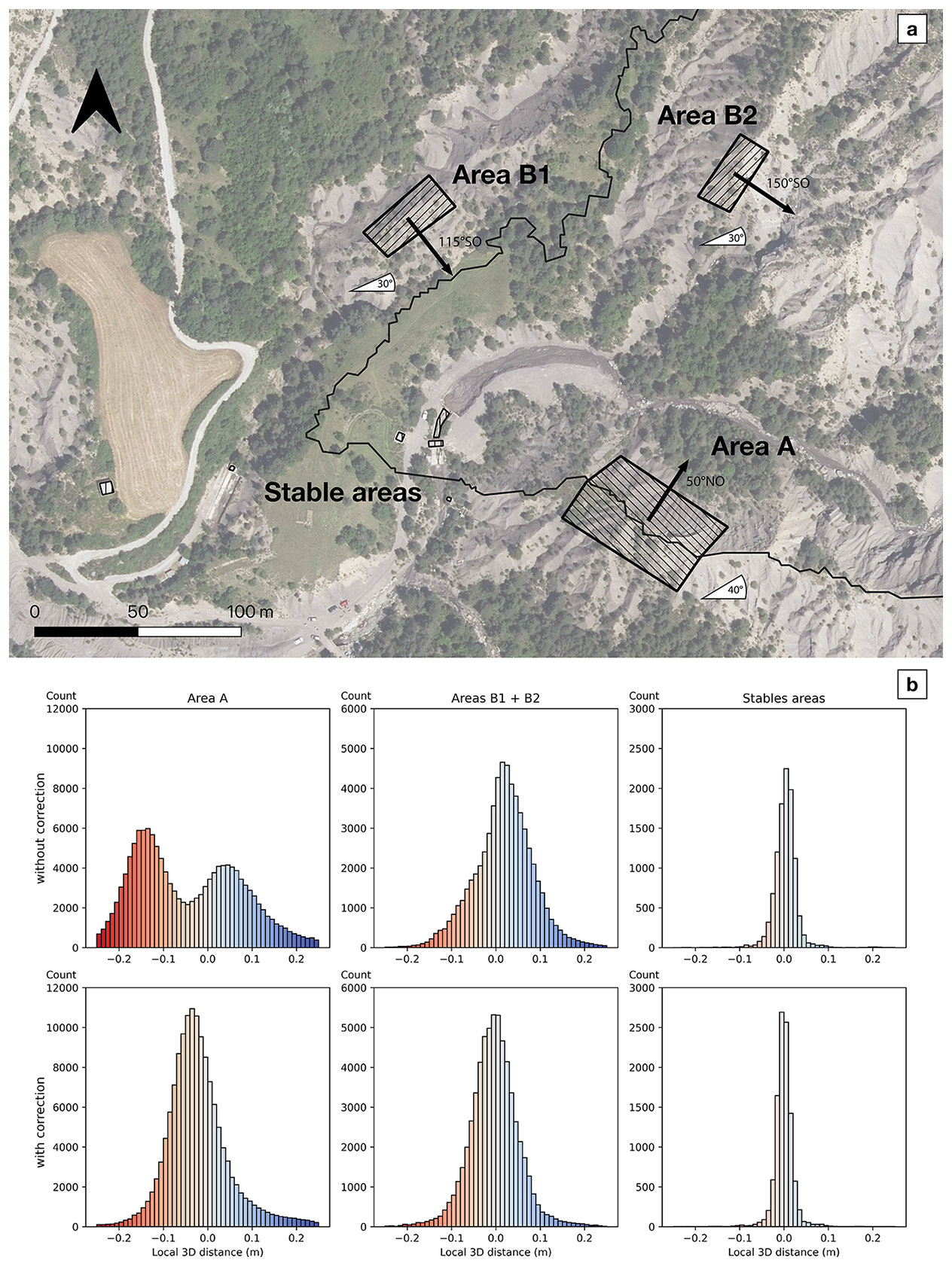
Figure D1 (a) Location of the study areas used to characterise the effect of a centimetric co-registration error between two campaigns. Background: Aerial photograph of the outlet of the Draix-Laval basin (IGN, 2021). (b) Distribution of local distances between ground points of the 2021 campaign and the 2015 campaign on the study areas with or without a $(\mathrm{\Delta }X,\mathrm{\Delta }Y,\mathrm{\Delta }Z)=(\mathrm{10},\mathrm{11},\mathrm{0.5})$ corrective shift (in centimetres) of the 2021 point cloud.