Rainfall and tectonic forcing lead to contrasting headwater slope evolutions

Landscapes evolve through the coupled effects of tectonics and surface processes. Previous studies have shown that uplift rate changes generate upstream-migrating erosion waves, altering downstream slopes while upstream slopes remain constant until the wave arrives. However, the distinctive differences between landscape responses to uplift versus climatic changes, particularly rainfall rate changes, remain incompletely described. This study uses a numerical model to investigate landscape responses to changes in both rainfall and uplift rates. Results show that, unlike the simple upstream-migrating erosion waves from uplift rate changes, rainfall rate changes generate more complex responses. Specifically, rainfall rate changes cause transient slope change reversals at the headwaters due to differential erosion between the divide and its adjacent areas, a pattern not observed in uplift-induced evolution. These reversals are more pronounced when hillslope diffusion plays a dominant role. While both rainfall and tectonic forcing drive landscape change, they produce recognizably different signatures in river profiles. If these distinctive signatures can be identified from river profiles or inferred from erosion rate measurements, they can help disentangle climatic and tectonic influences on landscape evolution.

1 Introduction

Whilst tectonic and geodynamic forces generate longer wavelength topography, Earth's surface processes powered by climate dissect the Earth's surface, creating high-frequency topographic features that contribute to the reconfiguration of drainage patterns and the re-routing of sediments from source to sink (e.g., Allen, 2008; Wobus et al., 2006a; Whipple et al., 2013; Martinsen et al., 2022; Seybold et al., 2021). Whether or not climatic and tectonic disturbances impact landscape evolution differently has been debated for decades (e.g., Kirby and Whipple, 2012; Whipple, 2009; Bonnet and Crave, 2003; Whittaker, 2012). Previous research has focused on various landscape features, such as river channels, drainage divides, and alluvial fans, to understand whether they respond differently to tectonic and climatic disturbances (e.g., Leonard and Whipple, 2021; Mao et al., 2021; Shi et al., 2021; Willett et al., 2014). Rivers, in particular, have been found to respond strongly to climatic and tectonic disturbances, making them a valuable feature for studying how landscapes evolve (e.g., Molin et al., 2023; Quye-Sawyer et al., 2021; D'Arcy and Whittaker, 2014). Here, we investigate via numerical experiments how river channels respond to rainfall and uplift, paying particular attention to the role of hillslope diffusion, which is often overlooked in favour of river incision processes. We show that river channels respond slightly differently to tectonic and rainfall-driven changes when hillslope diffusion is considered. After changes in uplift rate, the channel slope at the headwaters records a monotonic increase (uplift rate increase) or decrease (uplift rate decrease). In contrast, after changes in rainfall rate, the channel slope records a non-monotonic adjustment, which becomes more pronounced as the surface diffusion coefficient increases. We suggest that changes in rainfall rate cause a transient spatial variation in erosion rate around the divide area due to the interaction between hillslope diffusion and river incision. This difference has the potential to distinguish between tectonic and climatic influences on landscape evolution.

1.1 River incision vs hillslope diffusion

Several numerical models have been proposed to quantify river incision processes (e.g., Dietrich et al., 2003; Howard and Kerby, 1983; Perron et al., 2008). The most commonly used is the detachment-limited stream power model, which assumes that sediments are instantly flushed from the channel and that the bedrock erosion rate E depends on the channel slope S, drainage area A, and precipitation P:

$$\begin{array}{}\text{(1)}& E=k_{\mathrm{d}}(PA{)}^m{S}^n\end{array}$$

where m and n are positive constant exponents, and k_d is a coefficient describing the erodibility of the channel bed and reflects the combined impacts on the erosion of climate, lithology, bedload, and other potential parameters (Kirby and Whipple, 2012; Smith et al., 2022; Whipple and Tucker, 1999). Equation (1) simplifies the impact of climate on erosion by focusing only on mean rainfall rate. However, real landscapes respond to climate change not only through shifts in mean precipitation but also through (i) the distribution of storm magnitudes, (ii) the phase of precipitation (snow vs. rain) that controls the timing of snowmelt runoff (Meira Neto et al., 2020), and (iii) the dominant runoff-generation mechanism (Uhlenbrook et al., 2005). Moreover, incision in channels is often controlled by erosion thresholds (DiBiase and Whipple, 2011) and may be further moderated by vegetation–evapotranspiration feedbacks (Yetemen et al., 2019). While these factors are critical for site-specific predictions, Eq. (1) is used here to isolate the first-order impact of a change in fluvial erosion efficiency on landscape form, providing a baseline for understanding these more complex interactions.

Following the principle of conservation of mass, the rate of surface elevation change $(\partial z/\partial t)$ is determined by the difference between the uplift rate U and erosion rate:

$$\begin{array}{}\text{(2)}& {\displaystyle \frac{\partial z}{\partial t}}=U-E\end{array}$$

As rivers incise, the sloping ground at their flanks increases, driving hillslope diffusion, which describes the downward transport of creeping soil (Fernandes and Dietrich, 1997; Dietrich et al., 2003). Models indicate that the convexity of the hillslope profile is influenced by hillslope processes and the rate of incision at the hillslope base (e.g., Armstrong, 1987; Ahnert, 1987). Hence, river incision and hillslope diffusion are coupled and evolve simultaneously. A simple model describing the process of hillslope diffusion assumes that the flux of soil along hillslopes is linearly related to the hillslope gradient (e.g., Culling, 1963, 1960; Salles and Duclaux, 2014; Tucker and Hancock, 2010):

$$\begin{array}{}\text{(3)}& {\displaystyle \frac{\partial z}{\partial t}}=k_{\mathrm{hl}}{\mathrm{\nabla }}^{\mathrm{2}}z\end{array}$$

where k_hl is the hillslope diffusion coefficient, which integrates climate, lithology, soil conditions, and biotic influences (Dietrich and Perron, 2006; Hurst et al., 2013; Robl et al., 2017). Hillslope diffusion is the result of a combination of multiple near-surface processes: (i) rainsplash and sheet-flow creep driven by raindrop impact and overland flow (Guy et al., 1987; Meyer et al., 1975; Young and Wiersma, 1973), (ii) soil creep produced by cyclical wetting-drying, shrink–swell, and freeze–thaw strains (Anderson and Anderson, 2010), (iii) bioturbation by burrowing animals and tree throw that mix and move regolith (Gabet et al., 2003; Roering et al., 2010), and (iv) small shallow landslides that act diffusively when averaged over long timescales (Martin, 2000).

Climate controls the relative efficiency of these mechanisms. Mean annual precipitation and storm magnitudes regulate rainsplash fluxes and influence vegetation density, which in turn affects soil creep (Istanbulluoglu and Bras, 2006). Freeze–thaw frequency, governed by temperature and moisture, dictates the rate of frost creep and solifluction in high-altitude or high-latitude settings (Hales and Roering, 2007). Hillslope diffusion gradually transports soil and sediment downslope due to gravity and reshapes substantially the landscape over time (e.g., Litwin et al., 2025; Perron et al., 2008; Roering, 2008). It has been shown that hillslope diffusion strongly influences drainage density and valley spacing (Perron et al., 2008; Sweeney et al., 2015; Tucker and Bras, 1998). Additionally, the sediment and soil transported from hillslopes impact river incision by either acting as tools for erosion or forming a protective cover that shields the underlying bedrock from further erosion (Sklar and Dietrich, 2001).

While much research has focused on river channel evolution (e.g., Kirby and Whipple, 2012; Wobus et al., 2010), few have explored whether and how river channels respond differently to tectonic and climatic changes when hillslope diffusion is included. This knowledge gap exists in part because there is not yet a comprehensive theory describing how the hillslope diffusion coefficient changes with climate. Before addressing this issue, the following paragraph clarifies the notions of steady-state and transient landscapes.

1.2 Steady state vs. transient landscapes

Computer-generated landscapes evolving under controlled tectonic and climatic conditions provide a robust framework for better understanding the formation and evolution of natural landscapes (e.g., Chen et al., 2014; Pan et al., 2021; Salles and Hardiman, 2016; Schwanghart and Scherler, 2014). These models show that a landscape reaches a steady state when the uplift rate equals the erosion rate. When the uplift rate changes, landscapes are in a transient state of disequilibrium and evolve to reach a new steady state (e.g., Leonard and Whipple, 2021; Miller et al., 2012; O'Hara et al., 2019). Steady-state and transient landscapes show a sharp contrast in the morphology of river profiles. When a river channel has reached a steady state, its longitudinal elevation profile is usually smooth and concave-up (Fig. 1a). In contrast, under uniform lithology, knickpoints form in transient river channels (Wobus et al., 2006b; Lague, 2014; Neely et al., 2017; Whipple et al., 2013). A knickpoint is a location where there is an abrupt change in the channel slope (Fig. 1b). A positive knickpoint forms where the slope suddenly increases downstream, while a negative knickpoint forms where the slope decreases abruptly. A mobile positive knickpoint indicates an increase in uplift rate and/or a decrease in erosion efficiency (induced by a decrease in rainfall rate, for example), while a mobile negative knickpoint indicates the opposite conditions (Baldwin et al., 2003). Both types of knickpoints typically form at the river mouth and migrate upstream toward the headwaters.

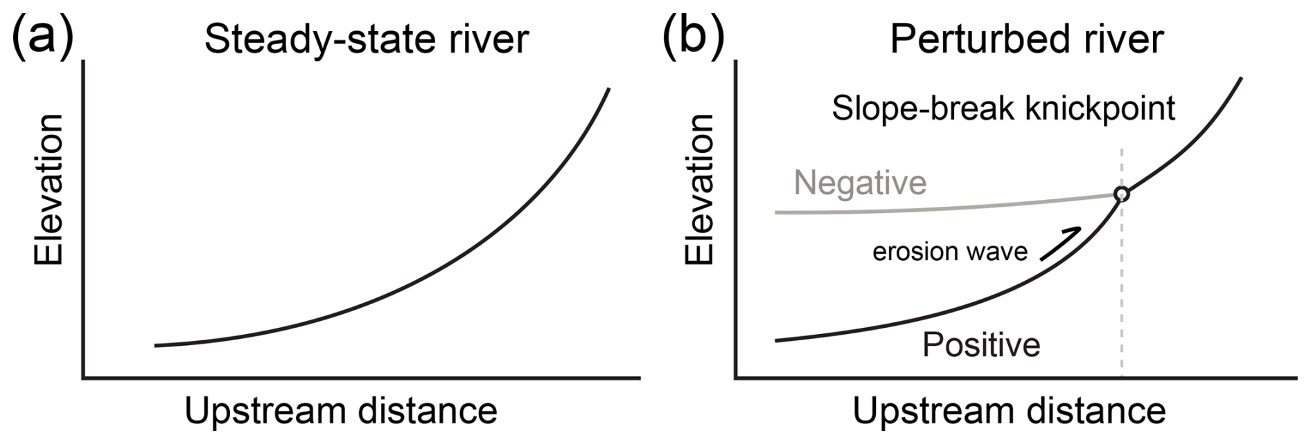
Figure 1 Channel profiles with different morphology. (a) A steady-state river profile. (b) Transient river profiles with a negative or positive slope-break knickpoint.

A migrating knickpoint separates the channel into two segments, upstream and downstream segments. It has been proposed that regardless of whether the transient change is driven by tectonics or climate, the elevation of the upstream segment changes while its slope remains constant (Whipple, 2001). After the downstream segment reaches a steady state, its channel elevation and slope have changed (e.g., Whipple, 2001; Whipple and Tucker, 1999).

2 Methodology and model setup

To investigate landscape evolution under climatic or tectonic changes, as well as varying erodibility and hillslope diffusion, we use the long-term surface evolution model Badlands (Basin and Landscape Dynamics) (Salles, 2016; Salles and Hardiman, 2016). Badlands can be used to simulate landscape development via the mobilisation of sediments through hillslope diffusion and stream-power incision. Our model assumes that hillslope sediment transport rates are linearly proportional to the slope gradient. Any material delivered to a channel cell from adjacent hillslopes increases the elevation of the cell. The river then erodes this new surface as if it were bedrock, without distinguishing it from the underlying substrate. Here, we explore landscape responses to changes in rainfall or uplift, and we disregard isostatic re-adjustment. In particular, we focus on contrasts in average elevation, surface roughness, and river profiles.

Our initial landscape models are mapped over a 40 km × 80 km grid with a uniform initial elevation of 10 m and a spatial resolution of 400 m × 400 m. We acknowledge that our 400 m grid spacing is larger than hillslope lengths in many natural landscapes. However, a sensitivity test at a finer 200 m resolution confirmed that our primary findings are robust and not an artifact of the chosen grid size (Figs. S1 and S2 in the Supplement). We design four initial models with varying hillslope diffusion and erodibility coefficients (Table 1). The diffusion coefficient is set to 0 in model M1, meaning the landscape evolution is purely driven by riverine processes with an erodibility coefficient of 2.3 × 10⁻⁶ yr⁻¹. We set the diffusion coefficient to 1 m² yr⁻¹ in model M2 and 2 m² yr⁻¹ in model M3. Finally, in our last model M4, the erodibility is doubled to 4.6 × 10⁻⁶ yr⁻¹. In all cases, the stream-power law uses m = 0.5 and n = 1.0.

Table 1 Diffusion coefficient, erodibility, and initial Pe of four models.

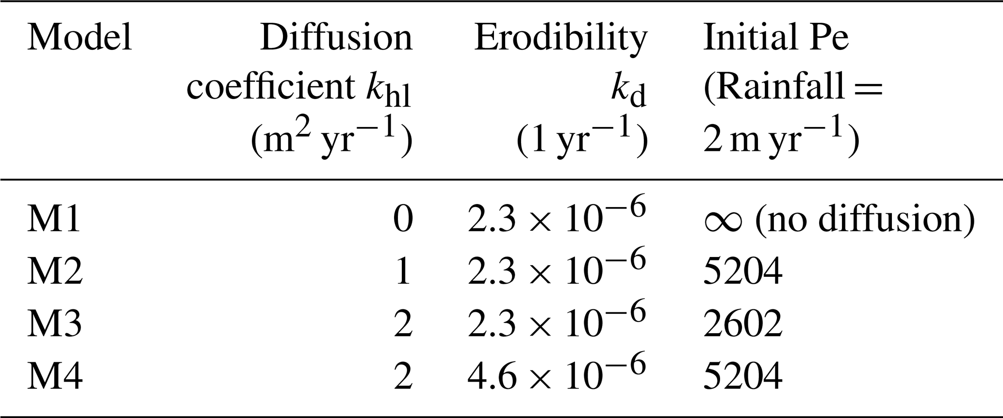
For each model, we compute the dimensionless parameter Pe to combine two a priori independent parameters (the diffusion coefficient k_hl and the erodibility k_d) into a single dimensionless measure of process competition (Bonetti et al., 2020; Perron et al., 2008; Perron et al., 2009):

$$\begin{array}{}\text{(4)}& \mathrm{Pe}={\displaystyle \frac{k_{\mathrm{d}}{P}^m{l}^{\mathrm{2}m+\mathrm{1}}}{k_{\mathrm{hl}}}}\end{array}$$

Pe is analogous to a Péclet number, which is the ratio of a diffusion timescale to an advection timescale (Perron et al., 2008). Low Pe values indicate diffusion-dominated systems, while high values indicate advection-dominated systems. We take the characteristic horizontal length scale l to be 40 km, representative of the real landscape. Based on our parameter values, model M3 has the lowest Pe, indicating that diffusion is more dominant in this model than in the others. Furthermore, models M2 and M4 share the same Pe because their parameters for k_hl and k_d are both doubled in M4 relative to M2, keeping their ratio constant.

Our four models are submitted to a combination of uniform uplift at a rate of 300 m Myr⁻¹ and background rainfall at a rate of 2 m yr⁻¹ until they reach a steady-state equilibrium, where mean elevation and river profiles no longer change (Montgomery, 2001; Willett and Brandon, 2002). This first stage lasts for 25 Myr (Fig. 2), after which all models reach a steady state.

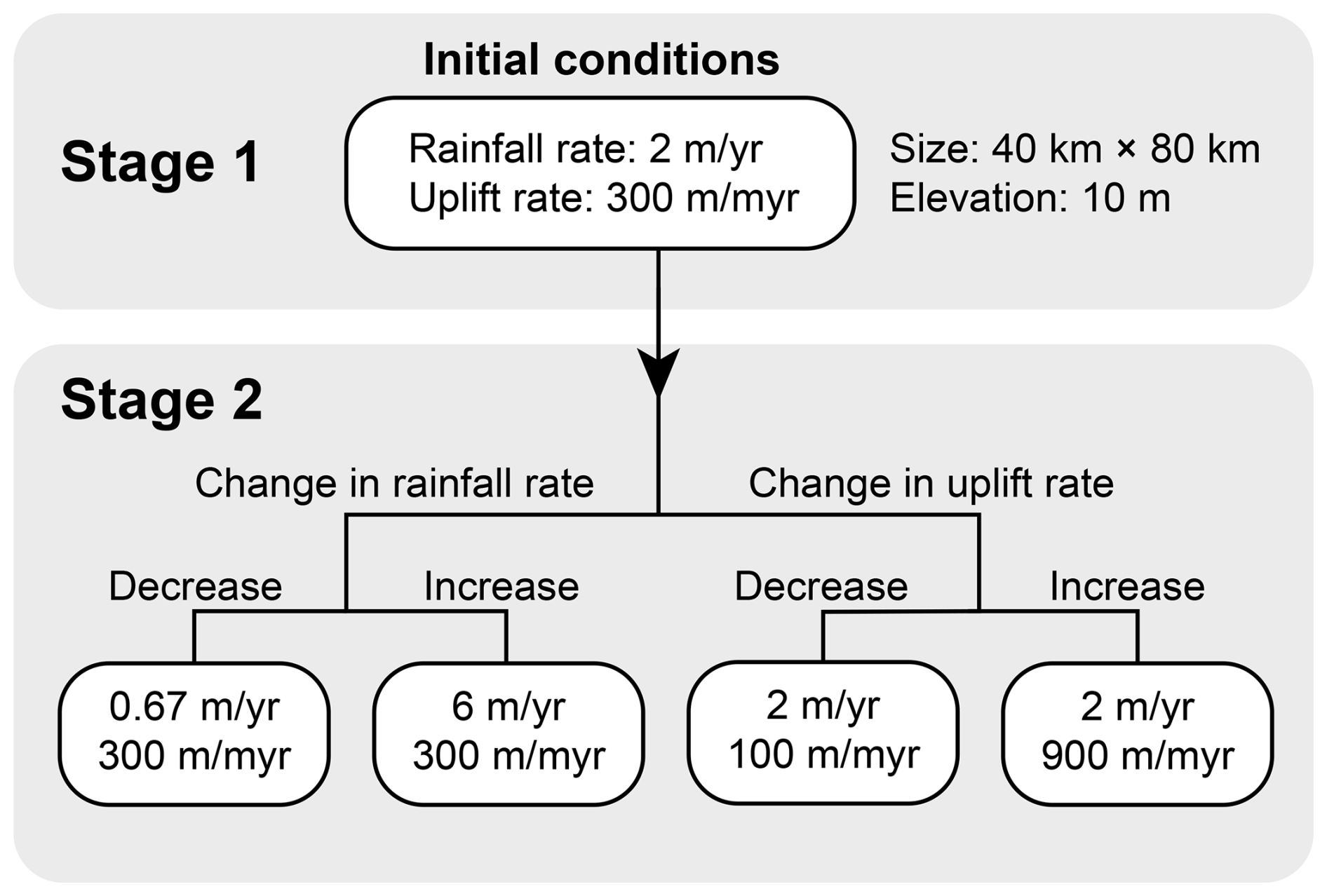
Figure 2 Each of our four initial models (M1 to M4) experiences four different two-stage landscape evolutions controlled by changes in rainfall or uplift. Stage 1: An initial flat landscape is uplifted under an uplift rate of 300 m Myr⁻¹ and a rainfall rate of 2 m yr⁻¹ until a steady-state landscape is reached. Stage 2: Changes in rainfall or uplift rate.

In the second stage, which also lasts 25 Myr, each model is subjected to a perturbation while the other forcing remains constant. We either:

• Increase rainfall to 6 m yr⁻¹ or decrease it to 0.67 m yr⁻¹, while keeping uplift fixed at 300 m Myr⁻¹, or

• Increase uplift to 900 m Myr⁻¹ or decrease it to 100 m Myr⁻¹, while keeping rainfall fixed at 2 m yr⁻¹.

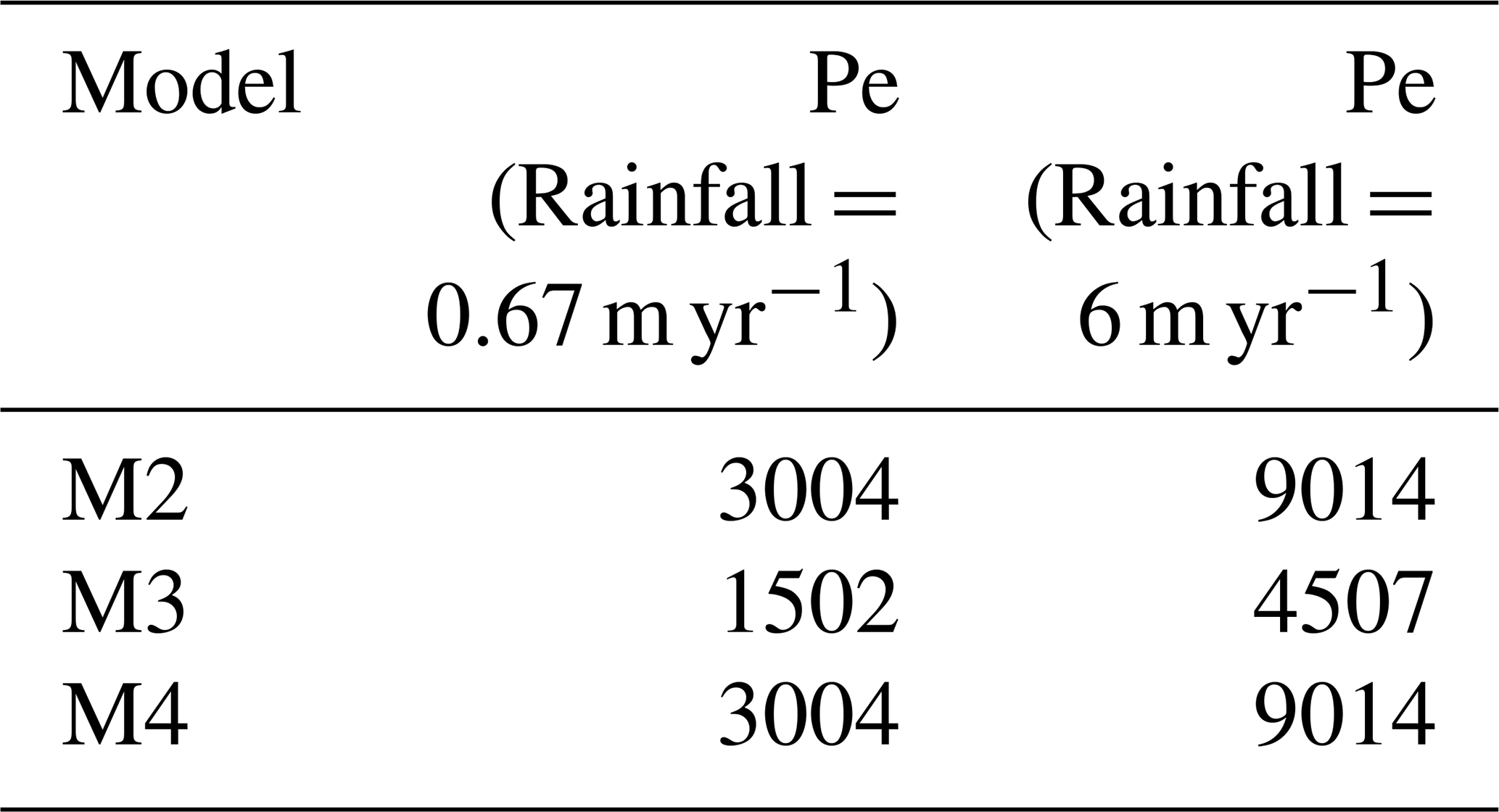
This design yields 16 individual experiments (Fig. 2), allowing us to assess landscape responses to changes in rainfall and uplift rates separately. A key consequence of our experimental design is that a change in rainfall rate directly changes the advection timescale associated with river incision. Thus, this changes Pe and alters the fundamental balance between advective and diffusive processes, as shown in Stage 2 (Table 2).

Table 2 Pe for Stage 2 rainfall-change scenarios.

3 Results

3.1 Comparison of final, steady-state landscapes

To quantitatively compare landscape responses across our experiments, we compute two metrics: mean landscape elevation and surface roughness. Mean landscape elevation serves as an integrated measure of the overall erosional state of the landscape, reflecting the cumulative effect of tectonic uplift, channel incision, and hillslope processes on topographic development. Surface roughness quantifies the local topographic variability resulting from the competing effects of processes that create and destroy relief (Doane et al., 2024). We calculate roughness as the difference between the maximum and minimum elevation values within a defined neighborhood surrounding each central pixel using the “roughness” algorithm of GDAL in QGIS (Wilson et al., 2007).

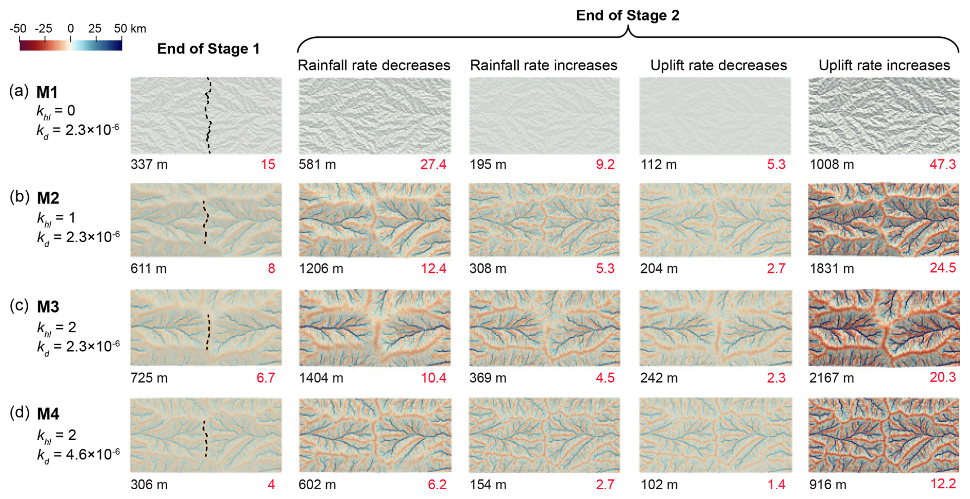
Figure 3 Hillshade maps showing cumulative erosion and deposition resulting from hillslope diffusion at the end of Stage 1 and the end of Stage 2 for models M1 (a), M2 (b), M3 (c), and M4 (d). Each model differs in hillslope diffusion coefficients (k_hl) and erodibility values (k_d). Blue areas indicate deposition, while red areas represent erosion. Color bar values indicate cumulative depositional (positive) and erosional (negative) amounts (km). Numbers below each map display the mean elevation (black) and roughness (red). Dashed lines on maps at the end of Stage 1 denote the divides. The divides in Stage 2 are similar to those in Stage 1 and are not marked in this stage.

Our results show that the mean landscape elevation and surface roughness increase following a decrease in rainfall rate or an increase in uplift rate, and decrease following an increase in rainfall rate or a decrease in uplift rate. Regardless of rainfall or uplift changes, the absence of hillslope diffusion in M1 (k_hl = 0) leads to the largest surface roughness (Fig. 3a). When hillslope diffusion is included, the landscapes in models M2, M3, and M4 are smoother than those in model M1 (Fig. 3b–d). For models M2 and M4, doubling both the diffusion and erosion coefficients reduces both the mean elevation and the mean surface roughness by a factor of ∼ 2. For models M2 and M3, doubling only the diffusion coefficient reduces the surface roughness by ∼ 15% and increases the mean elevation by ∼ 20%. For models M3 and M4, doubling the erosion coefficient alone reduces the mean elevation by a factor of more than 2.

Stronger diffusion smooths local slopes but also increases the flux of material into valleys. In our detachment-limited model, any material added to the channel from hillslopes is treated as bedrock, meaning the river must incise through it with the same efficiency as the underlying rock. To maintain equilibrium with a constant uplift rate, the river must therefore steepen to gain the power needed to erode both the uplifted bedrock and the additional material load (Litwin et al., 2025). This behavior represents an amplification of the channel gradient response, as the channel must become steeper than if the hillslope material were treated as easily erodible sediment. As stronger diffusion widens valley spacing and forces channels to steepen, the total relief and mean elevation of landscapes increase.

3.2 Impact on river channel response

To explore channel responses to changes in rainfall or uplift rates under various ratios of hillslope diffusion to erodibility, we analyze the trunk stream of the western basin, including the evolution of erosion and deposition, as well as the evolution of the longitudinal channel profile. Although we present results only from the western basin, we have verified that both drainage basins exhibit similar evolutions.

3.2.1 Null-case control (Model M1, k_hl = 0)

To isolate the impact of hillslope diffusion, we first present the results from model M1, which has a diffusion coefficient of zero and serves as our null case (Fig. 4). This model illustrates the baseline landscape response when driven purely by riverine processes, showing the development of a standard migrating knickpoint. By establishing this null case, we can then clearly distinguish the critical role of hillslope diffusion in landscape evolution in models M2, M3, and M4.

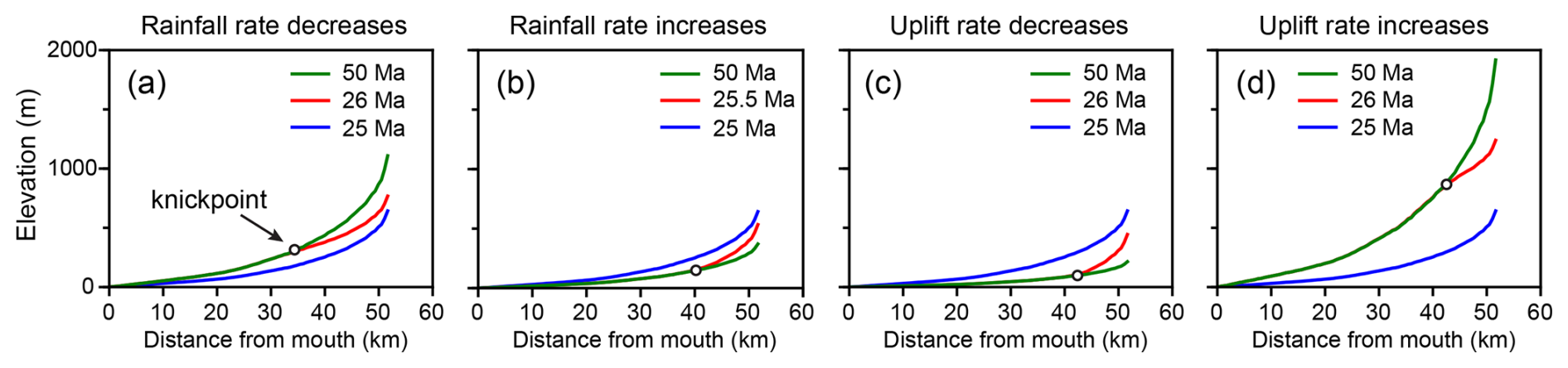
Figure 4 Longitudinal profiles of the trunk stream after changes in rainfall or uplift rates in model M1 (no hillslope diffusion). The changes occur at 25 Ma, affecting the steady state trunk stream in blue.

In the absence of hillslope diffusion, when the rainfall rate decreases or the uplift rate increases, the trunk stream rises gradually, and the slope increases from the river mouth. A positive knickpoint and an erosion wave develop at the river mouth and migrate upstream (Fig. 4a and d). The downstream channel reaches a steady state first, with no further changes in elevation or slope. Conversely, when the rainfall rate increases or the uplift rate decreases, the channel's elevation and slope decrease. A negative knickpoint and an erosion wave develop at the river mouth and migrate upstream (Fig. 4b and c). Once the erosion wave reaches the headwaters, the knickpoint disappears, and the entire channel returns to a new steady state. Notably, within 1–2 Myr of the change in rainfall or uplift rates, the channel elevation at the headwaters changes, but the slope remains nearly constant (Figs. 5a1–a3 and 6a1–a3). As the erosion wave approaches the headwaters, the channel slope increases or decreases monotonically and eventually stabilizes.

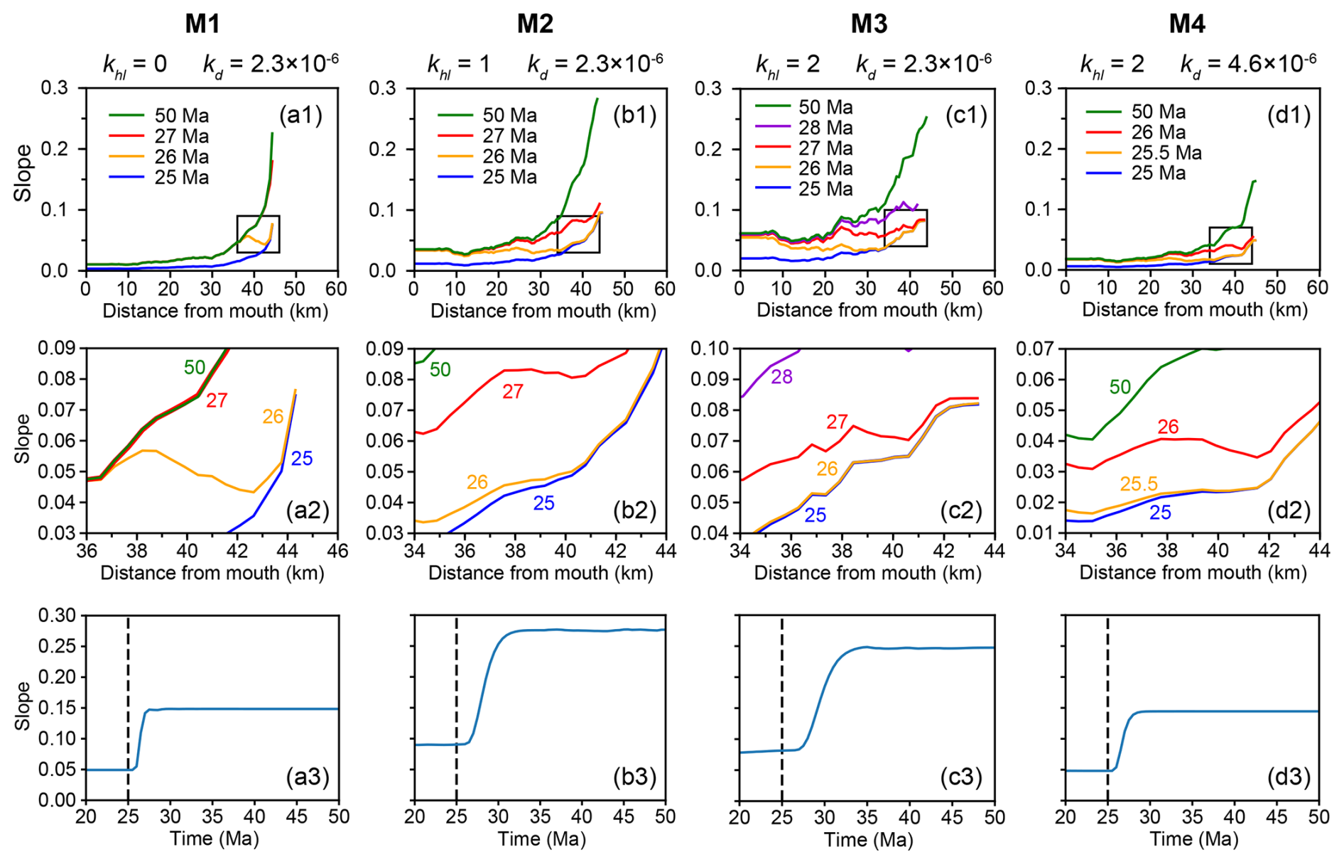
Figure 5 Evolution of trunk stream slope following an increase in uplift rate. (a1–d1) Longitudinal slope profiles of the trunk stream at selected time steps (colored lines), with each subplot corresponding to a model (M1–M4). Black rectangles indicate the headwater regions. (a2–d2) Enlarged views of the headwater areas, corresponding to the boxed regions in panels (a1)–(d1). (a3–d3) Temporal evolution of the mean channel slope in the upper ∼ 800 m of the trunk stream, capturing the dynamic slope response across model runs. Dashed vertical lines mark the timing of the uplift rate increase (25 Ma).

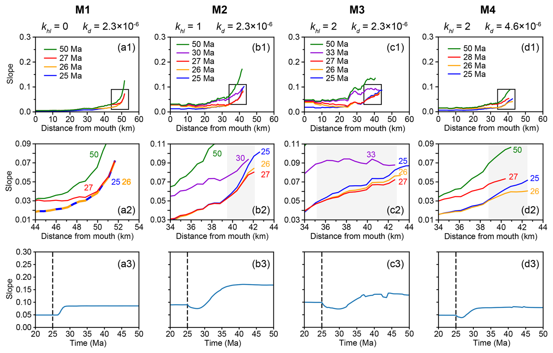
Figure 6 Evolution of trunk stream slope following a decrease in rainfall rate. (a1–d1) Longitudinal slope profiles of the trunk stream at selected time steps (colored lines), with each subplot corresponding to a model (M1–M4). Black rectangles indicate the headwater regions. (a2–d2) Enlarged views of the headwater areas, corresponding to the boxed regions in panels (a1)–(d1). Grey bands indicate the regions where the transient slope change reversal occurs. (a3–d3) Temporal evolution of the mean channel slope in the upper ∼ 800 m of the trunk stream, capturing the dynamic slope response across model runs. Dashed vertical lines mark the timing of the rainfall rate decrease (25 Ma).

3.2.2 Diffusion-enabled models (M2–M4)

In contrast, when hillslope diffusion is present (models M2, M3, and M4), we observe major differences in the evolution of headwater channel slope following changes in uplift and rainfall rates. An increase in uplift rate leads to a monotonic slope increase in the headwaters (Fig. 5b1–b3, c1–c3, and d1–d3). In contrast, a decrease in rainfall rate triggers a “transient slope change reversal”, a phenomenon we define as a non-monotonic adjustment where the headwater channel slope initially changes in the opposite direction of its final steady state. This is observed as a transient slope decrease followed by a subsequent, long-term increase (Fig. 6b1–b3, c1–c3, and d1–d3). The opposite pattern occurs when the rainfall rate increases: a temporary slope increase is followed by a decrease. We do not find a distinct threshold for the initiation of the transient slope change reversal; rather, it is present whenever hillslope diffusion is active (Pe < ∞). The primary control on the reversal is its magnitude and persistence, which vary continuously with Pe. Our results show that landscapes with lower Pe values, where hillslope diffusion is more dominant relative to channel incision, exhibit more pronounced and persistent reversals. For example, model M3, which has the lowest Pe, shows a reversal that persists longer and extends over a longer channel segment compared to other models (Fig. 6c1–c3). Although models M2 and M4 share the same Pe value, the larger k_hl and k_d values of model M4 halve both the diffusion and advection timescales relative to model M2. Consequently, the transient slope change reversal persists longer in model M2 in time, even though the non-dimensional dynamics are identical (Fig. 6b3 and d3).

4 Discussion

4.1 Mechanism of transient slope change reversal

To better understand the cause of the transient slope change reversal, we calculate the erosion rate for each grid cell 1 Myr after the disturbance and extract the erosion rate along the trunk stream for all models (Fig. 7). The transient slope change reversal is driven by differential erosion rates between the divide and adjacent areas.

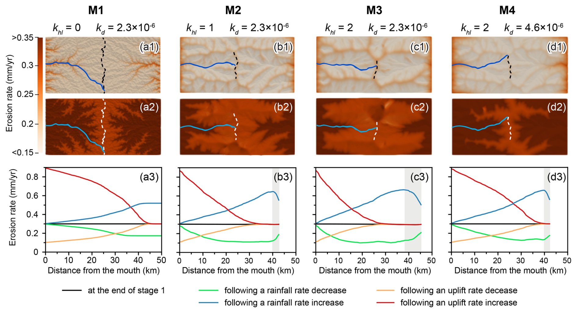
Figure 7 Erosion rates (mm yr⁻¹) per grid cell, calculated over 1 Myr following (a1–d1) a decrease in rainfall rate and (a2–d2) an increase in uplift rate. Blue lines in panels (a1)–(d1) and (a2)–(d2) represent trunk streams, and dashed lines mark divides. (a3–d3) Longitudinal erosion profiles along trunk streams, with grey bands indicating the regions where the transient slope change reversal occurs.

In model M1, the erosion rates of the divide and its adjacent areas remain homogeneous following changes in rainfall and uplift rates (Fig. 7a3). Similarly, in models M2, M3, and M4, an increase or decrease in uplift rate results in consistent erosion rates between the divide and adjacent areas (red and orange profiles in Fig. 7b3, c3, and d3). The surface uplift rate is defined as the difference between the uplift and erosion rates. Given the spatial uniformity of uplift rates, equal erosion rates at the divide and its adjacent areas result in identical surface uplift rates, preventing transient slope change reversals (black and red profiles in Fig. 8).

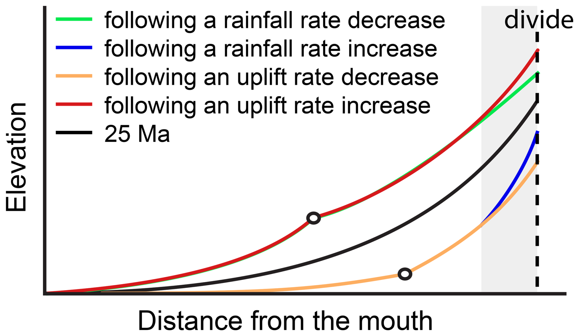
Figure 8 Schematic diagram of the longitudinal profile of the channel in a steady state (black line) or a transient state after changes in rainfall or uplift rate. The grey band indicates the region where the transient slope change reversal occurs.

In contrast, following a decrease in rainfall rate in models M2, M3, and M4, the erosion rate of the divide exceeds that of adjacent downstream areas (green profiles in Fig. 7b3, c3, and d3). This difference in erosion rate directly causes the surface uplift rate of the divide to be lower than that of adjacent downstream areas, resulting in a temporary decrease in the channel slope at the divide and, therefore, triggering a transient slope change reversal (green profile in Fig. 8). Conversely, following an increase in rainfall rate, the erosion rate of the divide is lower than in adjacent areas (blue profiles in Fig. 7b3, c3, and d3), causing a temporary slope increase at the divide and again triggering a transient slope change reversal (blue profile in Fig. 8). These findings suggest that rainfall changes distinctly influence divide erosion patterns, with spatial contrasts in erosion rate playing a key role in driving transient slope responses.

The transient slope change reversal is driven by a disequilibrium between the hillslope diffusion timescale and the channel advection (incision) timescale. Pe quantifies the ratio of these two timescales. Following a change in rainfall rate, the advection timescale, which is inversely related to incision efficiency, adjusts almost instantaneously. In contrast, the diffusion timescale, governed by topography, does not (Clubb et al., 2019). This abrupt shift in their ratio (i.e., the change in Pe) creates a lag and drives the transient behavior at the headwaters. For instance, following a decrease in rainfall rate, the advection timescale lengthens (river incision becomes less efficient) due to lower discharge (Mitchell, 2020; Montgomery et al., 2000). However, sediment continues to diffuse from divides to channels at a rate set by the pre-existing topography (i.e., the diffusion timescale is initially unchanged). This imbalance causes the rate of sediment supply from hillslopes at the headwaters to exceed the rate of sediment removal by rivers, reducing the channel slope temporarily and causing a transient slope change reversal. As the channel adjusts and the erosion wave migrates upstream, this reversal gradually disappears.

In contrast, a change in uplift rate uniformly raises the entire landscape without immediately affecting the efficiency of diffusion and incision. Because both the divide and its adjacent areas experience similar erosion conditions under constant discharge, no transient slope reversal occurs.

Notably, a lower Pe value amplifies the imbalance between sediment supply from hillslopes and removal by rivers. This enlarges the zone where divide erosion rates differ from downstream areas. Therefore, the transient slope change reversal persists over a longer channel segment and for a longer duration, as observed in model M3 (Fig. 6c2 and c3). In contrast, increasing Pe enhances river incision, which reduces the relative influence of diffusion. This leads to a shorter channel segment experiencing transient slope change reversal and a shorter duration of the transient response in model M4 (Fig. 6d2 and d3).

In summary, the transient slope change reversal results from the competition between incision and diffusion following a change in rainfall. This reversal disappears as the erosion wave gradually approaches the divide area, and the landscape returns to a steady state where the erosion rate is spatially uniform.

4.2 Field and analytical approaches for detecting transient reversals

Transient slope change reversals could be identified using slope-area analysis or χ analysis. Both methods rely on the stream power model, which describes the relationship between channel slope and drainage area as a power function (Flint, 1974). For a river channel in a steady state, plotting log slope against log area yields a straight line. However, in cases of transient slope change reversals, this relationship may deviate from linearity. While slope-area analysis can be sensitive to data noise (e.g., DEM inaccuracies), χ analysis reduces this influence through an integral approach (Royden and Taylor Perron, 2013; Perron and Royden, 2013). For steady-state rivers, χ should also correlate linearly with elevation, whereas nonlinear χ-elevation relationships may indicate transient slope change reversals. In our models, a decrease in rainfall rate produces a localized flattening at high χ (headwaters), directly reflecting the transient slope-change reversal (Fig. 9). By contrast, in uplift-driven transients the χ-elevation profile bows downward at low χ, while the high-χ (headwater) segment remains straight and is simply translated upward. However, χ-elevation analysis has limitations: it requires a steady-state baseline profile to distinguish different types of disturbances. Therefore, χ-elevation is best used in concert with additional information, such as independent erosion-rate measurements, to robustly identify and attribute transient slope-change reversals.

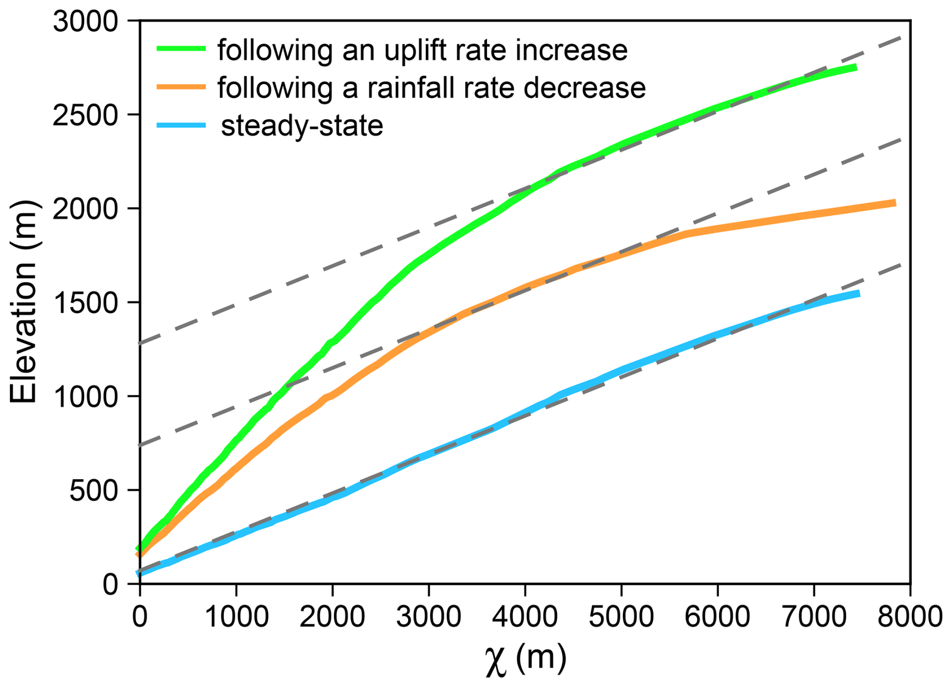
Figure 9 χ-elevation profiles of trunk streams in model M3 under three conditions: following an uplift rate increase (green), following a rainfall rate decrease (orange), and steady-state (light blue). The three grey dashed lines are parallel reference trends. χ-elevation profiles are calculated using a reference concavity index (θ_ref) of 0.4.

Transient slope change reversals could also be identified by investigating the erosion rate. One approach to quantify erosion rates is using cosmogenic nuclides, particularly radionuclides like ¹⁰Be and ²⁶Al (e.g., Balco et al., 2008; Gosse and Phillips, 2001; Lal, 1991; Muzikar, 2009). These nuclides are produced in surface minerals by cosmic ray interactions, with production rates decreasing exponentially with depth due to cosmic ray attenuation (Dunai, 2010; Lal, 1991). Cosmogenic nuclide concentrations increase as a surface remains exposed to cosmic rays (Ivy-Ochs and Kober, 2008). In contrast, in rapidly eroding areas, nuclide concentrations remain low due to the continuous removal of surface materials.

By mapping nuclide concentrations, spatial patterns in erosion rates could be linked to rainfall or uplift changes. For instance, if the erosion rate is relatively uniform around the divide area, it may suggest a transient response driven by tectonic events. Conversely, if nuclide data indicate that erosion rates are larger at the divide relative to downstream areas, then recent drainage reorganization may be related to a decrease in rainfall rate. Thus, cosmogenic nuclide measurements provide a valuable tool to distinguish between climatic and tectonic drivers of landscape change.

4.3 Model limitations

In this study, we aim to explore the first-order impact of hillslope diffusion and river incision on landscape and consider a landscape evolving under the action of hillslope diffusion and river incision only. While the linear diffusion model is a common starting point, we acknowledge that it does not capture nonlinear processes, such as those driven by shallow landslides, which can become significant on steeper slopes (e.g., Jiménez-Hornero et al., 2005; Martin, 2000; Roering et al., 1999). Furthermore, our model does not account for potential feedback between climate and the diffusion coefficient itself. In natural settings, the hillslope diffusion coefficient can vary with climatic conditions via processes such as frost-crack weathering, and near-surface processes such as soil saturation, and root growth (Braun, 2018; Perron, 2017; Bogaard and Greco, 2015; Andersen et al., 2015; Gabet and Mudd, 2010; Gabet, 2000). Considering this feedback could introduce additional complexity. For instance, an increase in rainfall rate could increase the hillslope diffusion coefficient through higher soil moisture (Perron, 2017), potentially amplifying the transient slope change reversal. Conversely, a decrease in rainfall rate could decrease the hillslope diffusion coefficient and dampen the reversal. Future work could explore the parameter space where these feedbacks become significant.

In addition, our use of a detachment-limited stream power model simplifies the complexities of sediment flux. The “transient slope change reversal” we observe is fundamentally a result of a disequilibrium between hillslope sediment supply and the channel's transport capacity following a change in rainfall. A more complex model incorporating sediment transport dynamics (a “transport-limited” or “mixed” model) would likely modulate the magnitude and duration of this reversal.

5 Conclusion

Changes in rainfall and uplift rates induce different responses in the channel slope at the headwaters, with hillslope diffusion playing a crucial role in mediating these processes. When the rainfall rate changes, hillslope diffusion interacts with river incision to generate transient spatial variations in erosion around the divide area, leading to transient slope change reversals at the headwaters. In contrast, changes in uplift rates result in spatially uniform erosion across the divide area, preventing such reversals. Identifying these reversals from river profiles or erosion rate estimates at different locations could help determine the driving force behind landscape adjustments. A high hillslope diffusion coefficient increases both the duration and spatial extent of these reversals along the river profile. In contrast, higher erodibility enhances river incision and diminishes the role of diffusion, reducing these reversal effects.

Our findings provide new insights into how rainfall and tectonic forcing reshape landscapes over time. By investigating the interaction between diffusion and incision, we show that the transient variations in channel profiles, particularly near the divide, provide potential markers for interpreting past landscape evolution and deciphering the complex interplay between tectonic uplift and climatic variability.