Automatic detection of floating instream large wood in videos using deep learning

Instream large wood (i.e. downed trees, branches, and roots larger than 1m in length and 10 cm in diameter) performs essential geomorphological and ecological functions that support the health of river ecosystems. However, even though its transport during floods may pose risks, it is rarely observed and remains poorly understood. This paper presents a novel approach for detecting floating pieces of instream wood in videos. The approach uses a convolutional neural network to automatically detect wood. We sampled data to represent different wood transport conditions, combining 20 datasets to yield thousands of instream wood images. We designed multiple scenarios using different data subsets with and without data augmentation. We analysed the contribution of each scenario to the effectiveness of the model using k-fold cross-validation. The mean average precision of the model varies between 35 % and 93 % and is influenced by the quality of the data that the model detects. When using a 418-pixel input image resolution, the model detects wood with an overall mean average precision of 67 %. Improvements in mean average precision of up to 23 % could be achieved in some instances, and increasing the input resolution raised the weighted mean average precision to 74 %. We demonstrate that detection performance on a specific dataset is not solely determined by the complexity of the network or the training data. Therefore, the findings of this paper could be used when designing a custom wood detection network. With the growing availability of flood-related videos featuring wood uploaded to the internet, this methodology facilitates the quantification of wood transport across a wide variety of data sources.

1 Introduction

Instream large wood includes downed trees, root wads, trunks, and branches that are at least 10 cm in diameter and 1 m in length (Platts et al., 1987). It is typically recruited from forested areas within the river catchment through natural tree mortality, wind storms, snow avalanches, wildfires, landslides, debris flows, bank erosion, and beaver activity (Benda and Sias, 2003). Stored wood within the river corridor plays a crucial role by trapping sediment, creating pools, and generating spatially varying flow patterns (Keller et al., 1995; Andreoli et al., 2007; Wohl et al., 2018). Therefore, instream wood is a crucial driver of river form and function and positively influences the diversity of the river ecosystem (Wohl et al., 2017). Although beneficial for biodiversity, wood can also be a hazard. During floods, large quantities of transported wood may accumulate at bridges or narrow river sections, blocking channels and causing localized inundations (Lucía et al., 2015). Additionally, the accumulation of wood can damage or even destroy bridges (Diehl, 1997; Lyn et al., 2003; De Cicco et al., 2018; Pucci et al., 2023). Costly wood removal efforts have long been the default mitigation strategy (Wohl, 2014), often without considering the ecomorphological impact (Lassettre and Kondolf, 2012; Collins et al., 2012). However, these preventive efforts can sometimes be counterproductive. For example, natural wood accumulations upstream of infrastructure can trap additional wood transported during high-flow events, preventing it from accumulating at critical infrastructure downstream (Ruiz-Villanueva et al., 2017). A more complex river system resulting from instream wood can also dissipate more flood energy than a channelized river (Curran and Wohl, 2003; Hassan et al., 2005). Human influence has impacted wood regimes and the river ecosystem through infrastructure development, channelling, and wood removal from rivers (Wohl et al., 2019). Therefore, it is crucial to understand instream large-wood dynamics by assessing the quantity (i.e. wood supply and storage), transport, and/or fluxes. In addition to direct monitoring and crowdsourced videos of floods, recent advancements in understanding large-wood dynamics have emerged through experimental flume studies and numerical studies (Panici, 2021; Innocenti et al., 2023). Estimating the quantity of wood in river systems and its temporal variation has gained traction over the last few years. However, in-field wood transport data remain scarce. As wood is mainly transported during floods, observations of transported instream wood are rare, and very few rivers are currently being monitored for this purpose (Ghaffarian et al., 2020, 2021). Different techniques can help assess a river's wood regime in terms of transport, such as radio-frequency identification (RFID), high-resolution aerial surveys, and video monitoring (MacVicar et al., 2009). With RFID tags, individual pieces of wood are assigned a unique identity, and their movement can be registered and tracked. RFID tags can be used to quantify the percentage of wood that moves each year (Schenk et al., 2013). Attaching GPS loggers to pieces of instream wood is expensive and limited in temporal range, but it can provide temporal data with a high frequency during high-discharge events (Ravazzolo et al., 2015). Aerial data can detect stored wood and wood jams (Haschenburger and Rice, 2004; Lassettre et al., 2008; Sanhueza et al., 2019). However, the best methods for quantifying wood transport are video-based because such methods provide a high temporal and spatial resolution (Ghaffarian et al., 2020). Before the introduction of deep learning methods, conventional computer vision methods were used for object detection. These methods rely on feature extraction techniques, such as edge detection, background subtraction, template matching, and histograms of oriented gradients (HOGs) (Zou, 2019). Edge detectors use pixel-based filters to analyse changes in image intensity (Sun et al., 2022). They help detect the contours of an object. Background subtraction algorithms work well with static camera setups (Kalsotra and Arora, 2021). They model the background and subtract the background model from the current frame. Template-matching techniques involve overlaying a template image on top of the input image to find regions that match the template (Swaroop and Sharma, 2016). Much like edge detectors, HOGs extract features by counting the occurrences of gradient orientations in certain portions of the image (Dalal and Triggs, 2005). Although robust, they require careful tuning.

Using computer vision software combined with stationary cameras to detect wood transport has provided a first insight into river wood dynamics (Lemaire et al., 2015; Zhang et al., 2021). This approach uses spatial and temporal pixel-level analyses to, for example, detect features such as colours, edges, and moving objects. The first feature is a mask that identifies potential floating objects that differ in colour from the water's surface. Combining these features eventually allows us to ascertain the presence of wood in the images. Even though the approach's utility has been proven and this approach is used to extract images of wood from videos recorded at a few sites (Zhang et al., 2021), it still requires manual, site-specific tuning. It is purposefully designed for a specific site to increase performance. When creating a method for a specific location, this approach performs well on the data for which it was designed but becomes too specific and complex for generalizing across a wide variety of datasets. Furthermore, the current method requires the camera to be angled in a fixed position to extract the wood detection features, which decreases flexibility. Even when tuned to a specific location, its performance depends on seasonal and weather conditions (Ghaffarian et al., 2021). Furthermore, measuring stations are limited by their spatial locations and rely on specific installation setups prior to a wood-moving event.

Developments in mobile technology have enabled millions of people to use high-quality video cameras. During extreme weather events, videos of floods are often posted online, which can be an exciting source for wood transport analyses. Citizen science projects, such as the Argentinian “storm-chasing” project, have demonstrated the use of home videos in analysing hydraulic conditions during storms (Le Coz et al., 2016). Similarly, crowdsourced videos can be used to analyse wood regime characteristics (Ruiz-Villanueva et al., 2019). However, quantifying wood transport using videos recorded from non-fixed viewpoints presents a challenge as existing tracking methods have failed to analyse crowdsourced footage due to their dependence on a stationary camera angle. Manual detection and quantification of large wood have been conducted in previous studies (Ruiz-Villanueva et al., 2022); however, these processes are labour-intensive. Advances in machine-learning methods can be applied flexibly and could allow for widespread wood detection.

Convolutional neural networks (CNNs) have been identified as an effective method for object detection (Lecun et al., 2015), showing success in remote-sensing-based environmental-monitoring applications (Li et al., 2020). These methods have been utilized for various tasks, including segmenting tree trunks in urban areas (Jodas et al., 2021), detecting floating plastic debris in rivers (van Lieshout et al., 2020; Àlex Solé Gómez et al., 2022), and monitoring river flow (Dibike and Solomatine, 2001). In studies highlighting the potential of deep learning for detecting and classifying objects in fluvial environments, transfer learning was used to classify static, stored large wood in rivers using aerial imagery, achieving a recall rate of 93.75 %, to overcome data scarcity (Schwindt et al., 2024). Similarly, deep learning has proven effective in other aquatic contexts, such as fish species detection and weight estimation (Sokolova et al., 2023), further illustrating the adaptability of CNNs in riverine environments. However, the application of CNNs in automating floating-wood detection remains under-explored, which we attribute to a lack of uniform training data (Maxwell et al., 2018; Shorten and Khoshgoftaar, 2019).

In this study, we propose using a You Only Look Once (YOLO) CNN as a flexible first approach to analyse floating wood in videos from various sources, circumventing the limitations of current state-of-the-art wood detection algorithms, which are site-specific and require calibration. Our algorithm aims to detect and track floating wood pieces in any river, under various conditions, and from varying sources. Different video sources include permanent monitoring cameras and handheld devices belonging to witnesses of wood-laden flood events in rivers. This research offers immediate applications, such as computing wood fluxes to understand wood dynamics in rivers, as well as practical uses, including warning systems and flood hazard and risk assessments.

2 Methods

2.1 Selecting the convolutional neural network

Our convolutional neural network comprises multiple convolutional layers that analyse video frames. Convolutions are used to extract hierarchical features from images to make predictions (Lecun et al., 2015). Features such as edges, corners, and textures are combined to determine the class of an object. The algorithm learns which features are necessary for classifying an object as instream wood. These detection features do not require individual hard coding but are developed by training the network with class examples. Depending on its architecture, a CNN can thus be several orders of magnitude more complex and theoretically more effective at detecting wood. Training a CNN demands substantial data, ideally from diverse sources under varying weather and flow conditions (Bengio et al., 2013).

The main convolutional neural networks using deep learning include region-based convolutional neural networks (R-CNNs), the Single Shot MultiBox Detector (SSD), CenterNet, and the You Only Look Once algorithm. R-CNNs introduced the concept of region proposal networks (RPNs), which first extract a region of interest before classifying it (Ren et al., 2017). This two-step process generally results in longer processing times. The SSD method, in contrast, does not use the region proposal step but instead utilizes multi-scale feature maps (Liu et al., 2016). Another approach that omits the proposal stage is CenterNet, which identifies an object as a pair of key points representing the centre and size of the object (Duan et al., 2019). The YOLO algorithm features a unified architecture and detects objects, ranging from image pixels to bounding-box coordinates and class probabilities, as a single regression task. This enables the YOLO algorithm to excel in both speed and accuracy (Bochkovskiy et al., 2020). Its single-pass architecture allows it to consider the entire image context during the detection phase, which is advantageous for identifying multiple pieces of wood simultaneously (Redmon et al., 2016). Furthermore, the YOLO algorithm has undergone seven major updates over the past 6 years (Redmon et al., 2016; Wang et al., 2022). Such frequent updates and improvements can benefit the development of a wood detection method. Therefore, for the main part of this study, we chose to train the fourth generation of the You Only Look Once network.

2.2 Data

Training a convolutional neural network (CNN) that can detect wood under various conditions requires multiple steps. First, instream wood data are acquired and labelled. Subsequently, the dataset is trimmed and augmented to create a database of varying images containing instream wood. Once these steps are complete, a large part of the database is used to train the model, whilst a smaller part is used to validate the training performance. In this context, the term “database” refers to all the data used to create the CNN, whilst the term “dataset” refers to a subset of the database consisting of all the data recorded by one device at a specific location and on a specific date. Figure 1 provides an overview of the data collection and processing and demonstrates that we assess the performance of 14 different augmentation and sampling strategies from the datasets.

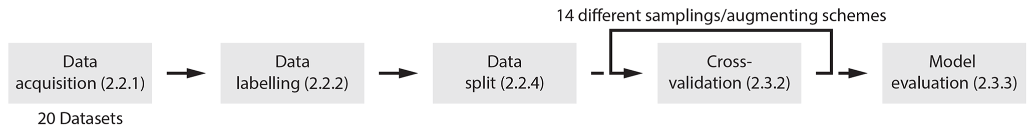
Figure 1 Overview of the methodology used for data collection and processing. Of the 20 labelled datasets obtained, 6 representative datasets were chosen for cross-validation (see Fig. 4).

2.2.1 Data acquisition

For this study, we employed five low-cost cameras that were available to the authors, including three Android phones and two Raspberry Pi camera modules. The cameras were temporarily installed at various locations, on different days, and at different times, with various orientations and resolutions (see Table 1). The cameras were mounted to bridges and other stationary structures using makeshift supports to ensure a stable vantage point for capturing video footage of the floating wood. This method allowed for flexibility in positioning the cameras at various angles, depending on the bridge and the river section being monitored. We manually introduced wood into the river upstream of the cameras and allowed them to record the wood passing by during a time window ranging from 30 to 90 min. We also used data from two locations in France, where permanent cameras have been monitoring the Allier River since 2019 and the Ain River since 2007 (Zhang et al., 2021; Hortobágyi et al., 2024). These data were used to analyse the wood flux and only contain natural instream wood occurrences. An operator-based visual floating-wood detection method was employed to detect the wood. Labels were already available; however, as the labelling process involved only labelling the new pieces in each frame, the labels were insufficient for the method proposed in this paper. To test the model's performance after optimization, we gathered a test dataset. The test dataset consisted of 281 images with a resolution of 1280×720 pixels, taken with a Xiaomi Mi 9 phone in time-lapse mode. These images were collected at the river Inn during an experimental flood at its tributary, the river Spöl. The River Ecosystems research group at the University of Lausanne has actively studied this location with respect to wood transport since 2018. It provides a valuable test dataset because an algorithm like ours could greatly reduce the human labour involved. Lastly, carefully selected images of floating wood were sourced from online repositories (purchased from http://istockphoto.com and http://dreamstime.com, last access: 1 March 2024) to represent a small but diverse floating-wood dataset. All images in this dataset are from different sources and various locations. Additionally, instead of being recorded by a camera attached to a bridge, these images were captured by photographers. When used as training data, this dataset helps increase the variety of data sources. When used as validation data, it serves as a benchmark for how well the model generalizes wood. The final database consists of 15 228 images, each containing one or more pieces of wood. The images are divided into 20 different datasets, 9 of which are shown in Fig. 2.

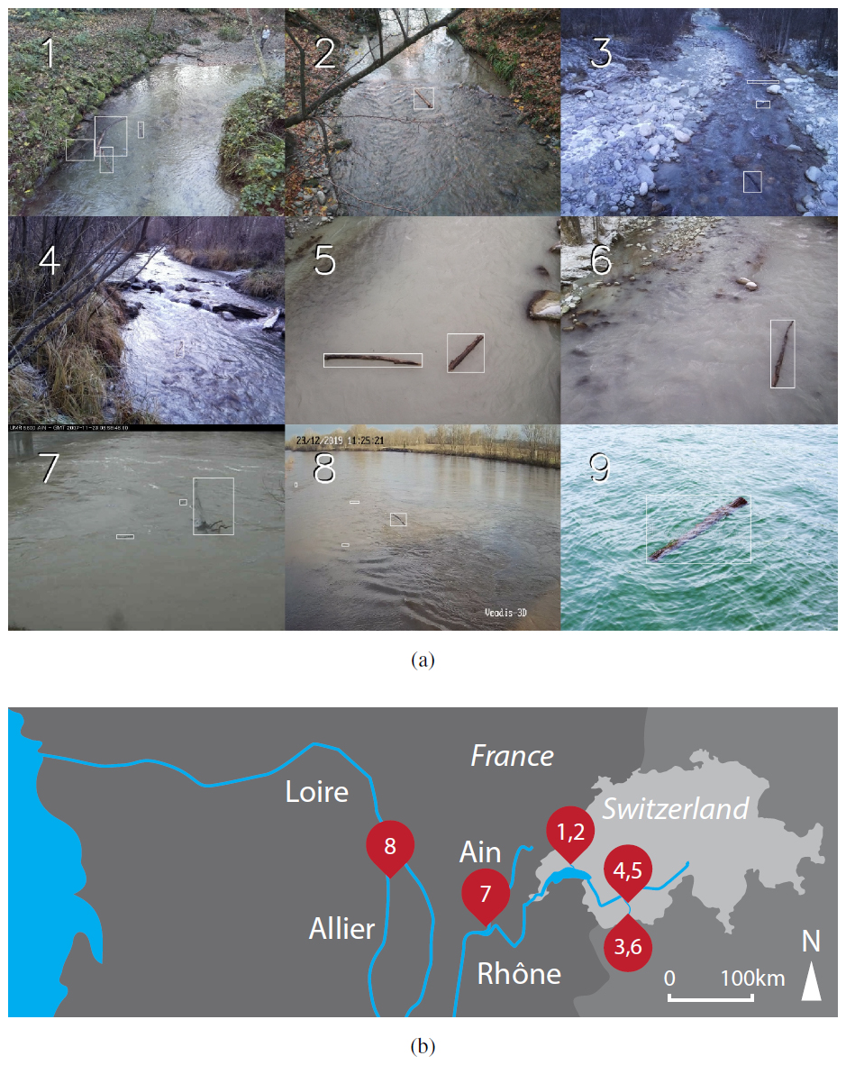
Figure 2 Examples from 9 of the 20 datasets. (a) Examples with bounding boxes around instream wood. (b) Locations of the datasets. Images 1 (46.52373° N, 6.57729° E) and 2 (46.52296° N, 6.57577° E) are of the river Chamberonne. Image 3 (46.04814° N, 7.48884° E) is of the Borgne d'Arolla. Image 4 (46.17966° N, 7.4187° E) is of the river Dixence. Images 5 (46.1612° N, 7.44079° E) and 6 (46.10975° N, 7.49428° E) are of the river Borgne. Image 7 is of the Ain River (image acquired by the École normale supérieure (ENS) de Lyon). Image 8 is of the Allier River (image acquired by the ENS de Lyon). Image 9 is of an unknown location (purchased from http://iStock.com, last access: 1 March 2024).

Table 1 Data acquisition statistics. For datasets 1–15, the devices were temporarily attached to bridges. Datasets 16–19 were collected from permanent monitoring stations. Dataset 20 consists of random samples found online.

^*Used as a representative dataset.

2.2.2 Data labelling

Using both manual and automated approaches, labels were created for the data acquired to indicate where an instream piece of wood is located within each frame. Each bounding box represents the four coordinates of a box's corners, which fit around the piece of wood (see Fig. 2 for examples of bounding boxes). Initially, the labelling was manually performed using labelling software called “LabelImg” (Viso.ai, 2022). To expedite the process, we devised a pseudo-labelling method. Only 10 % of the images in each dataset (1922 in total) were labelled by hand. A CNN (CenterNet; Duan et al., 2019) was trained to deliberately overfit this specific dataset by only using images from that particular dataset. Using the CNN, the labels for the other 90 % of the images were created. Subsequently, we verified that all bounding boxes correctly indicated a piece of wood and adjusted any incorrect labels by going through all the labels manually. It was verified that this method worked well in 11 out of the 15 cases in which we had abundant data and required minimal manual intervention. However, for the other four datasets, CenterNet's performance was not sufficient for labelling the other 90 % of the images as the mean average precision (mAP; see Sect. 2.3.3) was below 20 %. Therefore, it would have required too much time and effort to manually create a completely labelled dataset. Accordingly, only the hand-labelled 10 % of the images were used.

2.2.3 Data analysis

After labelling, we obtained 15 228 fully labelled video screenshots with bounding boxes (see Fig. 2) around 33 160 pieces of instream wood. When training a CNN, the goal is to have diverse data. Wood naturally floats and drifts with the current or becomes deposited and trapped by obstacles, such as riverbanks, boulders, and trees. As a result, some videos record the same piece of wood at the exact location for several minutes. Therefore, the data were trimmed. If, for subsequent frames, the labels that encompassed the identified pieces of wood were almost identical (with the location, width, and height of all bounding boxes being within a certain percentage of each other based on visual assessment), only one of the frames was kept in the database.

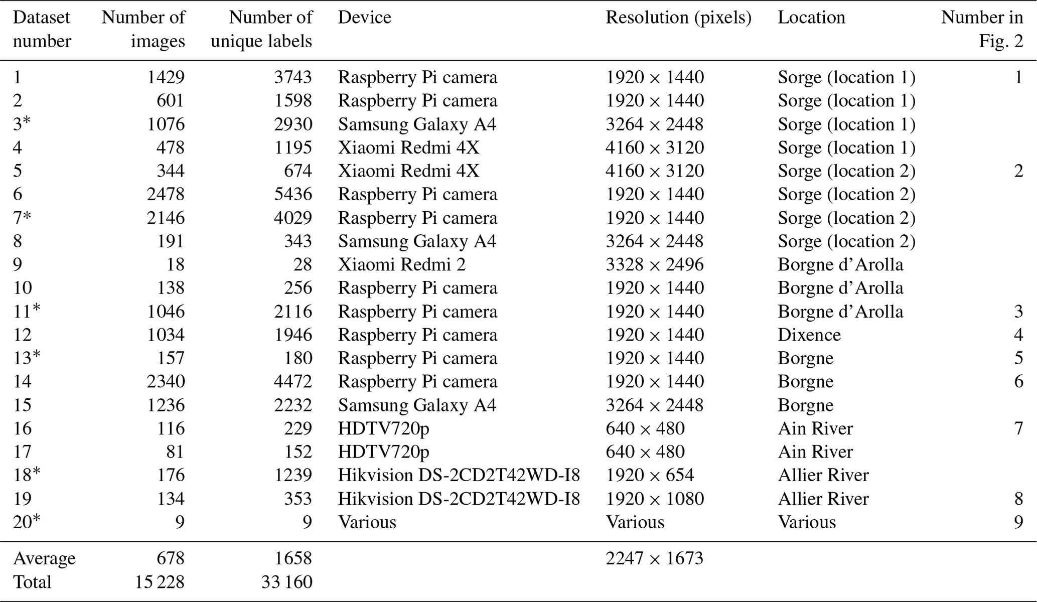
To prepare the data for analysis, all labels were cropped from their corresponding images in the database and resized to grey-scale images of a certain resolution. This resulted in a dataset consisting only of the pieces of wood cropped from the images (for an example, see Fig. 3). The pixel resolution was maximized to 80×80 pixels, the largest size at which all labels could be processed with the available random-access memory. This yielded images of all 33 160 pieces of wood in the database without their surrounding context. Subsequently, the images were normalized and centred to eliminate circumstantial and camera-specific white-balance differences. This meant that the average pixel intensity of each picture was set to 128 and that the maximum or minimum pixel values were adjusted to 255 or 0, respectively (see Fig. 3). To analyse the variance in the data and perform clustering in an unsupervised manner, we used a Python package called clustimage (Taskesen, 2021), along with custom scripts. The analysis consisted of dimensionality reduction and clustering. First, a principal component analysis (PCA) was applied to reduce the dimensionality of the data. High-dimensional data (80×80 pixels) were transformed into a lower-dimensional space while retaining 98 % of the original variance. This reduced the complexity of the dataset, making it more manageable for subsequent clustering. Following the PCA, we clustered the reduced dataset using a k-means algorithm. For four different instances with two, four, six, and eight clusters, respectively, the silhouette score was calculated to evaluate the similarity within the clusters compared to the dissimilarity across various clusters, effectively gauging the compactness and separation of the clusters.

Figure 3 (a) An original cutout and (b) a grey-scaled, normalized, and centred cutout recorded on 29 November 2020 (Raspberry Pi 4, image no. 7411, label 2).

After the principal component analysis, we performed t-distributed stochastic neighbour embedding (t-SNE). The stochastic nature of the t-SNE method meant that, although each run seemed to cluster similar samples, the exact output graph differed each time. Therefore, we used it for visual interpretation purposes only. Furthermore, we compared the relative sizes of the bounding boxes across datasets to understand the differences in the data.

2.2.4 Data split

Machine-learning data are typically split into training, validation, and test datasets. The training data are used to train the neural network to recognize patterns and make predictions. The validation data are used to tune the model's hyperparameters, ensuring it performs well on out-of-sample data. The test data are unseen data used to benchmark the final performance of the CNN (Xu and Goodacre, 2018). Usually, all labelled data are combined, after which a certain portion of the data, such as 90 %, are randomly assigned as training data, whilst the other 10 % are assigned as validation data. This ensures that the training and validation data represent the overall data.

In our case, however, as the data come from a limited number of sources with common locations and camera angles, splitting the data using traditional methods might cause overfitting, resulting in an overestimation of the model's performance. A model that overfits performs well on training data but poorly on unseen data because it has learnt the specifics of the training data too well. Multiple leave-one-out cross-validations can be used to mitigate overfitting, where one complete dataset is left out of the training data and used as validation data.

For feasibility purposes, six validation cycles were run. For each cycle, a single dataset was dropped for validation, whilst the model was trained on the remaining 19 datasets (see Fig. 4). Six representative datasets were chosen to ensure diversity in terms of location, camera angle, and time and to reduce computational overheads by avoiding 20 validation cycles. For each training scenario, the performance was averaged over the six runs. This process was repeated for 14 different training scenarios, as described in Sect. 2.3.2.

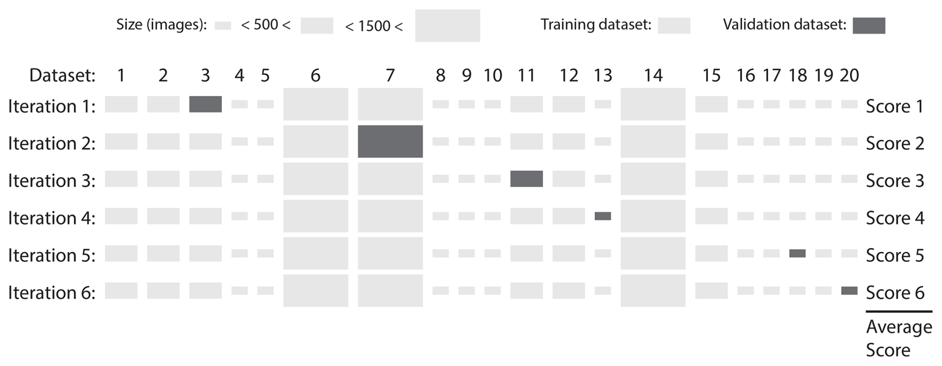
Figure 4 Cross-validation scheme for one training scenario. This figure shows the distribution between the datasets used for training and those used for validation. The y axis shows all available datasets, and the x axis shows the different training efforts. The dark-grey dataset represents the validation data, while the other 19 datasets were used to train the model. Ultimately, the six scores were averaged to produce the validation score. The size of the rectangle represents the size of the dataset.

2.3 Machine learning

2.3.1 Training data size sensitivity

Before attempting to enhance performance across various scenarios, we assessed whether the entire dataset was necessary for model training. It was hypothesized that reducing the training data might not compromise model efficacy and could potentially accelerate the training process. The 20 training datasets have an average size of 761 images and a median size of 411 images, with some datasets containing almost 2500 images. To reduce computational demands, we conducted tests to evaluate how the number of images sampled per dataset affects training performance. We conducted two tests with a 4-fold difference in the total number of training images compared. In the first test, 2000 images were augmented and sampled per dataset. Since the datasets did not all contain this exact number of images, they were randomly over or undersampled to reach this figure. During oversampling, no additional data were introduced; instead, this process ensured that the dataset sizes were equalized, thereby preventing biases in the rewards towards any particular dataset. We applied the same approach for the second test but used 500 images per dataset. Thus, the total training sample of 38 000 images (2000 images per dataset across 19 training datasets) for the first test was compared to the 9500 images for the second test (500 images for each of the 19 datasets). Following this comparison, we determined whether using a smaller amount of total data would decrease the model's performance.

2.3.2 Cross-validation procedure

When training the YOLO CNN, the training and validation images were downscaled to a resolution of 416×416 pixels as standard and consisted of three red–green–blue (RGB) colour bands. A series of experiments were conducted to enhance the model's performance. Including the baseline, 14 different testing scenarios were performed to test the model's sensitivity to stationary frames, dataset size, data augmentation, and data quality. As until this point, CNNs had not been trained for detecting instream large wood, thorough testing of different training strategies was crucial. To enhance model performance, the database size can be expanded by adding more labelled images or through the synthetic augmentation of existing data. Although more effective in image classification practices, augmenting data for object detection has been shown to improve model performance by up to 2.7 percentage points in mean average precision (mAP) in some cases (Zoph et al., 2020). The augmentation practice, however, attracts less research attention because it is considered to transfer poorly across different datasets. Apart from augmentation, employing various sampling strategies may also improve the algorithm's detection performance. The data used for wood detection can also exhibit diverse camera angles, pixel sizes, and proximities to the stream (see Table 1). To determine the most effective sampling and augmentation strategies for different data types, 14 models were trained and evaluated against a baseline model. The baseline model was trained using only the labelled images without any modifications. The other 13 scenarios are detailed below:

1. Trimmed – testing sensitivity to stationary frames. When labels were similar in at least three subsequent frames, the respective images were deleted from the database. Determining the exact pixels where a bounding box began and ended was sometimes challenging (e.g. when part of a log was underwater and its end was not clearly visible). As a result, bounding boxes around an immobile object could vary from frame to frame. To account for this, detections were considered similar when all bounding boxes were within 4 % of their subsequent x and y locations in the frame and within 30 % of their width and height. These thresholds were determined manually by testing various percentages in cases where multiple stationary logs were detected in successive frames. In this scenario, 13 375 images from the total database were kept.

2. Sampled (V1) – testing sensitivity to dataset size (“min500” and “max1200”). As small datasets can be undersampled compared to large datasets, in this scenario, we sampled a minimum of 500 images per dataset and a maximum of 1200 images per dataset. If the dataset contained fewer than 500 images, we oversampled images randomly and added duplicates to the dataset until we reached 500 images. We did not use all the data if the dataset had more than 1200 images. These numbers were chosen because, when applying this sampling method to the 20 datasets, the total number of labelled images was 15 257, similar to the total database size (15 228 images).

3. Sampled (V2) – testing sensitivity to dataset size (“750”). In this sampling scenario, to sample equally from all datasets, 750 images from each dataset were used. The total number of labelled images was 15 000, similar to the total database size (15 228 images).

4. Sampled (V3) – testing sensitivity to dataset size (“min500”). To avoid deleting data, in this scenario, only the small datasets were randomly oversampled to reach a size of at least 500 images. As all data from the other datasets were retained, the total dataset size was larger than that of the baseline.

5. Augmented (V1) – testing sensitivity to data augmentation (“mirrored rotated all”). To increase the diversity of the data, all images were used, and duplicates were mirrored and/or rotated. The rotation was kept between −15 and 15°; in practice, the river almost always appeared at the bottom of the frame. This was done because the data that needed to be analysed normally also included the river at the bottom of the frame. In this scenario, the dataset contained twice the number of images (30 456) as the baseline because each image was augmented randomly with a duplicate. Each image had a 50 % chance of being mirrored, so approximately 7614 images were mirrored, whilst all 15 228 duplicates were randomly rotated between −15 and 15°.

6. Augmented (V2) – testing sensitivity to data augmentation (“mirrored rotated randomly”). To increase the diversity of the data, the images were randomly selected to be mirrored and/or rotated. The rotation was kept between −15 and 15°. In 50 % of the cases, an image was mirrored (yielding a total of approximately 7.614 images), and in the other 50 % of the cases, the image was rotated randomly between −15 and 15°. The dataset for this scenario consisted of 15 228 images.

7. Augmented (V3) – testing sensitivity to data augmentation (“only mirrored”). The images were randomly mirrored in 50 % of the cases to disentangle the mirroring and rotation effects. The dataset for this scenario consisted of 15 228 images.

8. Augmented (V4) – testing sensitivity to data augmentation (“only rotated”). The images were randomly rotated between −15 and 15° in 50 % of the cases to disentangle the mirroring and rotation effects. The dataset for this scenario consisted of 15 228 images.

9. Added (V1) – testing sensitivity to data quality (high-definition, non-floating wood added). In an attempt to increase the model's understanding of wood, we added photos of instream wood lying in mostly dry riverbeds to the database. A total of 167 photos, each containing at least one wood sample, were added. The added data had pixel dimensions of 4608 by 3456 and were higher in quality than the other 20 datasets (see Table 1). Here, the influence of the bounding-box size and data quality was evaluated.

10. Added (V2) – testing sensitivity to data quality and diversity (12 datasets added). At a later stage in the testing process, a subset of frames from videos found online were labelled and added to the training database. A total of 10 datasets, ranging from 8 to 118 images per dataset, were added from locations in North America, New Zealand, and Switzerland. Additionally, two self-gathered datasets from different sources – containing 207 and 499 images, respectively – were added. As they were sourced from the internet, the 1206 images included in this scenario were compressed, with an average resolution of 1650×1133 pixels. Therefore, the quality of the added data was worse than that of the original 20 datasets. The added data are indicated by the letter “A” in Fig. 5. The “A11” and “A12” descriptors refer to the additional self-gathered datasets.

11. Removed – testing sensitivity to data quality (worst-performing datasets removed). As lower-quality data can weaken the model's understanding of wood, in this scenario, the quality of the data can be analysed by evaluating the effectiveness of the model trained in the base scenario in detecting samples. The two datasets with the smallest relative bounding-box sizes were assumed to include the fewest details and be of the lowest quality (see Fig. 5). The three lowest-quality datasets were datasets 12, 18, and 19. In this scenario, we removed datasets 12 and 19 from the training data to see whether the other datasets' detections improved. We considered dataset 12 to correspond to a location where large wood would unlikely be monitored. Additionally, as datasets 18 and 19 were taken from the same source and we wanted to maintain data variability, we did not remove dataset 18.

12. Merged – testing sensitivity to the addition of a time component (three images merged into one). Because the distinction between a piece of instream wood and flow features, such as eddies and waves, was often not clear from a single image, in this scenario, we merged three images into one image after converting them to grey-scale images. Therefore, instead of using regular red, green, and blue bands, the model was trained on grey-scale images at T−1, T, and T+1, with T representing the time step of detection. This approach was hypothesized to aid detection as waves and eddies change during a short time step, whereas wood does not.

13. Double resolution – testing the model's sensitivity to an increase in input image size (from 416 to 832 pixels). A CNN was trained based on a specific predefined image resolution. As standard, images were resized from a higher resolution (between 640×480 and 4160×3120 pixels; see Table 1) to a resolution of 416×416 pixels before being used for training and validation. Decreasing the image resolution may have resulted in a loss of detail, especially in cases where the relative sizes of the wood pieces were small. Therefore, we evaluated the model's sensitivity to input image size in this scenario by resizing the images to 832×832 pixels instead, retaining more details.

2.3.3 Model evaluation

Generally, a commonly used metric for object detection tasks used to evaluate performance is mean average precision (mAP) (Tian et al., 2024), which combines three different measures: precision, recall, and intersection over union (IoU) (Zheng et al., 2020). Recall refers to the percentage of wood pieces detected by the algorithm out of all the logs that pass by. Precision indicates whether the piece detected by the CNN was indeed instream wood. The object detection algorithm outputs either no bounding boxes or (multiple) bounding boxes for each image. Each bounding box indicates the outer limits of the object and has a confidence percentage corresponding to how certain the model is in its detection. Lowering the confidence threshold increases the number of bounding boxes classified as detections. Hence, recall increases, and precision decreases. The changes in precision and recall based on the threshold can be displayed in a precision–recall curve. The surface area under the curve can be translated into a single average-precision (AP) value for a specific IoU. However, this value does not compare different IoU thresholds. IoU compares the label with the detected bounding boxes by dividing their overlap by their combined total surface area. For each IoU value, a different precision–recall curve can be created, resulting in different APs. When all different APs, based on different thresholds and IoUs, were combined into a single value, we obtained the mAP, which ranged from 0 % to 100 %. With an upper mAP limit of 100 %, the model would label every instance of instream large wood in exactly the same way as the humans who labelled the training data. However, as human-performed labelling is imperfect, mean average precision is not an objectively perfect performance index.

Different applications of object detection call for different thresholds of recall, precision, and IoU, depending on the consequences. Depending on the large-wood regime of a specific river, more emphasis can be placed on either recall or precision. When the amount of wood passing through is very low, e.g. one piece of wood per month, increasing recall can ensure that no piece is missed. However, when sensitivity is set too high, the model may wrongly detect wood in every frame, forcing the user to look at every image and delete all the false detections.

We trained a model across all 14 training scenarios and validated it with the six validation datasets. The training was performed in epochs, representing the number of times all the training images were used to train the model. The model was validated using the validation data after a predetermined number of epochs had passed during the training process. The model's performance on the validation data was recorded in terms of mean average precision. During the same training session, the model may not only produce several tests that perform similarly but also exhibit an outlier in performance that cannot be reproduced. To account for this and avoid overestimating the performance, instead of only the single best, we used the two best mAP validation values to determine the performance of each training run. Furthermore, different training sessions using the same data can yield varying performance results as the model may converge to different local optima depending on the initialization and training dynamics. Therefore, we ran each test three times to compare different training scenarios. Hence, we obtained an average of the six best mAPs for each scenario.

Additionally, on a small subset of training scenarios, a newer YOLOv7 model was trained to compare the results of different models using the same data. A final model was then trained after determining which training strategies worked best for each data type. This model was tested on the test dataset described in Sect. 2.2.4, which had never been used in any of the analyses or training efforts. In this way, the test dataset represented a case in which an unrelated wood-monitoring study used the model for out-of-the-box detection.

Finally, neural networks for object detection are often considered black boxes, which decreases their trustworthiness. To increase transparency, algorithms were developed to reverse the detection process and identify the input pixels in the image that were weighted the highest when the process decided whether or not to detect an object. For the YOLOv4 algorithm, we used a Python package called YOLIME (Sejr et al., 2021) for this purpose. YOLIME explains YOLOv4's object detection using LIME (Ribeiro et al., 2016). For each prediction, LIME perturbs the input data and observes prediction changes to highlight the image pixels that most influence the wood detection outcome. This process makes YOLOv4's predictions more understandable and, therefore, more trustworthy. Various instream wood samples from the database were handpicked, and YOLIME was run to determine which pixels were most heavily used by the model to detect wood. The algorithm provided insights into which features of the image it identified as characteristic of a piece of floating wood. Combined with data quality analysis, this understanding can help explain variations in model performance across different training scenarios.

3 Results

3.1 Training data: diverse but still clustered

The data used in this research appeared to be diverse. The PCA (principal component analysis) yielded a low silhouette score, and a visual inspection of the t-SNE plot revealed only small clusters of similar data (see Appendix A2), suggesting the presence of duplicates within the data. However, the analysis also uncovered similarities within each dataset. A comparison of the average bounding-box sizes across datasets revealed distinct differences. Figure 5 illustrates the relative size of the bounding box compared to the overall image size, calculated by dividing the total number of pixels in the envelope of the bounding box by the total number of pixels in the image. The image highlights discrepancies in the sizes of labelled pieces of wood across different datasets. To adjust for the exponential distribution of calculated surface areas, we applied a square root transformation to the bounding-box area for better visualization. The graph indicates that datasets 12, 18, and 19 from the original database were lower in quality. This is because, in these cases, the sample sizes were small, and for datasets 18 and 19, the camera was also located relatively far away. Examples of the differences in bounding-box sizes between dataset 1 and dataset 12 are displayed in Figs. C1 and C2 in the Appendix.

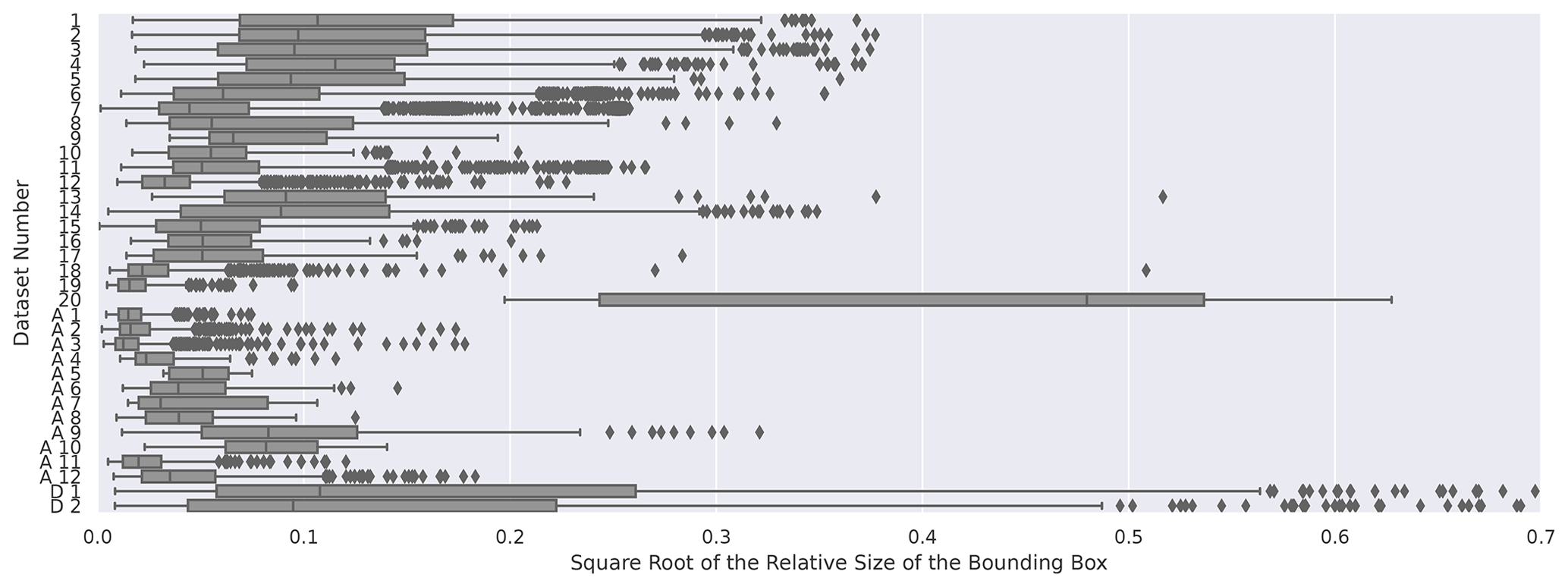
Figure 5 The relative sizes of the wood pieces compared to the image size for each dataset. The relative size is represented by the square root of the surface area of the bounding-box size divided by the square root of the total image size. The square root of the relative size is shown to facilitate the interpretation of the figure. The datasets from Table 1 are indicated by numbers. “A” indicates datasets added in scenario 10. “D” indicates datasets added in scenario 9.

Table 2 Neural-network performance for the base scenario in terms of mean average precision (mAP; see Sect. 2.3.3) and the relative change in mAP (expressed in percentage points) when using the 13 different training scenarios.

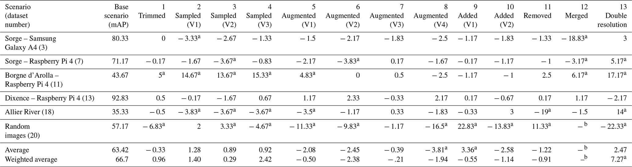
^a These values indicate mAP changes of more than 3 percentage points, whether positive or negative.
^b Dataset 20 does not contain a time series, so it cannot be merged.

3.2 Training results: database configuration matters most

Analyses showed that the model's performance did not increase when oversampling data from 500 (9500) to 2000 (38 000) images per dataset. The best mAP was similar for both tests. Figure 6 shows the difference between a training instance with 2000 augmented images per dataset (Fig. 6a) and one with 500 augmented images per dataset (Fig. 6b). It shows that increasing the data for a training instance slows down the model's convergence without increasing the eventual mAP.

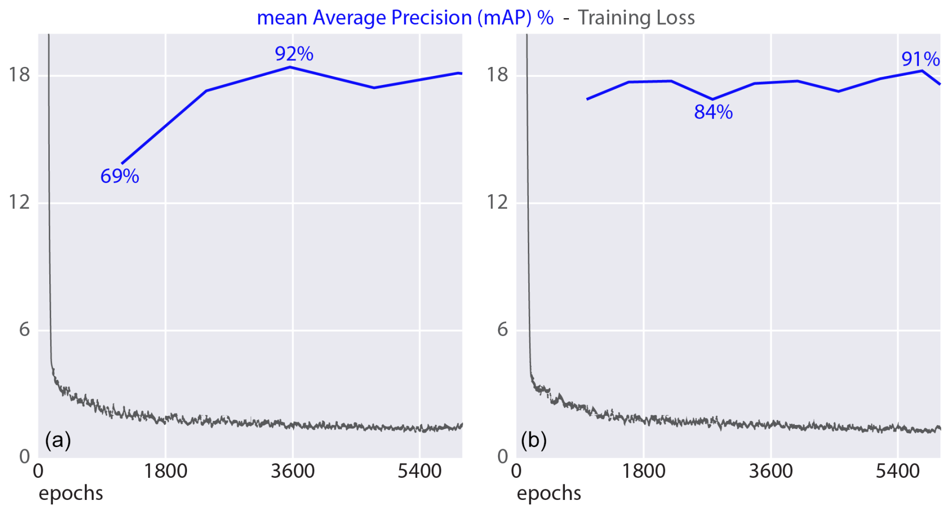
Figure 6 Training performance on dataset 13 (see Table 1) when using 2000 images (a) and 500 images (b) per dataset (38 000 and 9500 training images used, respectively). The blue lines denote the mean average precision, and the grey lines refer to the complete intersection-over-union training loss (Zheng et al., 2020).

Table 2 shows the training results for different scenarios. When using the total number of 15 228 labelled images, the average performance in terms of mAP was 63.42 %. The following columns show the difference in performance (mAP) between the base scenario and the 13 test scenarios, based on the six best performances. At the bottom of the table, the average of the six mAPs and the weighted average are shown. As there was large variation in the sizes of the datasets, to not overestimate the importance of small datasets, the weighted average compensated for the relative size of the datasets.

Dataset 20, despite its small size, exhibited large variability because the images were sourced from different locations. This variability makes this dataset particularly useful for assessing the model's ability to generalize the concept of wood and detect it across diverse conditions. On the other hand, the larger datasets include data recorded by cameras mounted on bridges and will, therefore, be a better representation of the primary use of the algorithm. Therefore, the weighted average is a better performance metric for the practical use of the algorithm.

Table 2 also shows the increase in model performance when changing the sampling strategy. When data from videos of floods featuring instream wood, sourced from YouTube and X (formerly Twitter), were added (scenario 10), the mAP for all datasets went down by 2.58 percentage points. This decrease in performance can arguably be attributed to the low quality of the data, which was confusing to the model. This observation was further supported by the reduction in performance in this scenario when validating the high-definition dataset of random wood images. Additionally, the model performed better when tested on the Allier River dataset, which mainly contains smaller (lower-quality) samples of wood (see Fig. 5). Instead of adding lower-quality data, we added high-definition data of non-floating wood to the training data (scenario 9). The significant increase in performance when validating dataset 20 can be explained by the algorithm's ability to generalize the concept of wood. This increased the average performance but decreased the weighted average performance as the overall average label sizes of dataset 20 were relatively small.

3.3 Test results

After analysing the scenarios, a novel test dataset (see Sect. 2.2.4) was introduced to evaluate the model's performance, recorded during a flood event at the river Inn (see Fig. 7). Notably, the model had never used this dataset during its training phase, and no adjustments were made to the hyperparameters based on these new data. The mean average precision (mAP) from the flood dataset was 61 % when using the base scenario. Increasing the input resolution of the model to 832×832 pixels, as per scenario 13, did not increase the performance (60.5 % mAP).

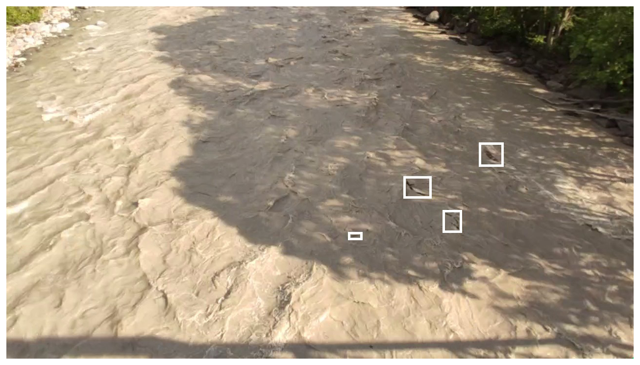
Figure 7 Example frame from the test dataset, collected at the river Inn in June 2023. The white bounding boxes enclose images of pieces of instream wood. A camera attached to a bridge recorded the scene in time-lapse mode.

4 Discussion

4.1 Effect of data quality on performance and sampling strategies

Our research led to the development of a comprehensive database containing labelled videos of instream wood. The labels covered a broad spectrum of sizes, particularly when comparing different datasets. They ranged from clearly identifiable downed trees with distinct features, such as bark, branches, and a brown colour, to bounding boxes resembling less-defined shapes that spanned only a few pixels in both dimensions. Additionally, distinguishing water waves and eddies from pieces of instream wood can sometimes be challenging during labelling as an image is only a snapshot. At the moment the image is taken, a wave ripple can resemble a piece of wood.

The model had a performance of 66.7 % mAP and therefore performs slightly better than the van Lieshout et al. (2020) model, with an approximately 50 % mean precision observed when creating a plastic detection algorithm and testing it on an unseen new location. Table 2 shows the results of the different training scenarios explained in Sect. 2.3.2. The sensitivity analysis indicated that increasing the dataset size to 2000 images per set did not enhance performance compared to when 500 images were used per set. This suggests that oversampling from a limited number of data sources does not improve model performance as the model tends to overfit specific instances. Consequently, when training a custom model or making future enhancements, utilizing 500 labelled images is sufficient. This threshold can optimize resource allocation and efficiency.

The proposed method does not require algorithm tuning for different sites, enabling its implementation across a range of different data sources. However, the training database, although extensive in size, is still limited in terms of the number of sources. The test with the best performance occurs during scenario 6 when using dataset 13. In this test, the model performed with a mean average precision (mAP) of 95.2 %. The model's worst performance occurred when dataset 18 and scenario 11 were used, with a mAP of 16.3 %. From this large difference in performance, it can be argued that data quality and diversity remain limiting factors of the approach. This conclusion is reinforced by a qualitative analysis of the quality of the datasets. As lower-quality data might confuse the model, scenario 11 was performed, excluding the lower-quality datasets (datasets 12 and 19) from the training data. The results (Table 2) show a weighted average decrease of 0.91 percentage points. This decrease is primarily linked to the worst performance of the model for the Allier River (dataset 18), where the decrease was large (19 percentage points) because the excluded dataset was taken from the same data source on a different day. Therefore, it can be argued that the model was still shown to overfit the training data, even with the precautionary measures. By reasoning the other way around, the −19 percentage points can be interpreted as +19 percentage points when adding data from the same scene recorded on another day. This particular removed dataset contained 176 images. Accordingly, this shows a more practical implication for researchers. When starting a new monitoring project, it is good practice to label and add as few as 200 images to the larger database. In this way, one can train a site-specific wood detection algorithm, which has been shown to perform better than the out-of-the-box model. The above findings also showed that, although the validation data used to calculate the mAP were taken from a data source other than the training data, there was still similarity. Data from the same camera recorded on different days, as well as data from the same location and date recorded with different cameras, were shown not to be completely different.

Additionally, the results showed that the model's performance increased when using different sampling strategies (scenarios 2, 3, and 4). This was primarily because the detection using dataset 11 as the representative dataset was more accurate. Dataset 10 was recorded from the same camera angle at a different time. The scene looked different, with a sunny background and sharp shadows, compared to the evenly lit, overcast conditions of dataset 11. However, oversampling the 138 labelled images from dataset 10 positively affected the model's performance on dataset 11 in all three scenarios. This underlines the need for the careful sourcing of training datasets and shows the influence of dataset sizes. The model has been trained to optimize performance on all training data and will, therefore, be biased towards the larger datasets. For the model to detect wood across a wide variety of scenes during the training phase, it is helpful to have equal dataset sizes, whilst a custom model for detecting wood from a single camera angle can benefit from oversampling from that specific scene. Furthermore, the data trimming from scenario 1 seemed to have a limited effect.

In scenarios 5, 6, and 7, data augmentation was applied to introduce variability in the form of mirroring and slight rotations. Scenario 5 mirrored and rotated all images, with rotations ranging from −15 to 15°, while in scenario 6, images were rotated and mirrored randomly. In scenario 7, 50 % of the images were randomly mirrored without rotation. The results show that scenario 7, with only random mirroring, had the least negative impact on model performance, yielding a minor change of −0.39 percentage points in the weighted mAP and even showing a slight improvement for certain datasets. In contrast, scenarios 5 and 6 resulted in slightly larger decreases in performance (mAP changes of −2.08 and −2.45 percentage points, respectively). These findings suggest that the rotation of the images, in particular, negatively impacts the model's performance as it might introduce distortions.

The results of scenario 12, where we merged three frames into one to integrate a time component, yielded interesting insights. For datasets where the model had already demonstrated robust performance, the accuracy experienced a noticeable decline. On the other hand, for datasets where the initial model struggled, an improvement of 6.2 percentage points was observed. This suggests that incorporating temporal information might be particularly beneficial when distinguishing between subtle features, such as pieces of wood and waves, proves challenging for a single frame. Further investigation into the impact of this temporal integration is needed to understand the specific scenarios where this approach is advantageous. These findings underscore the potential of leveraging temporal information to improve river wood detection.

Another adjustment to the method was evaluated in scenario 13, where we doubled the image size after rescaling. This scenario demonstrated its greatest improvements in performance on the three datasets with the lowest relative bounding-box sizes among the six representative datasets (datasets 7, 11, and 18; see Fig. 5). This indicates that the reduction in image size was too extreme, and some samples may have been missed. For custom detection algorithms, it is advisable to calculate the relative bounding-box sizes of the samples for their specific locations and optimize the image rescaling in terms of performance and computational efficiency.

For the model's mean average precision of 61 % on the test dataset (for the river Inn), it is essential to highlight that this accuracy was achieved despite the size of the Inn being larger than that of most rivers in the training database, the flood event's challenging conditions, and the relatively low quality of the imagery. Images with dimensions of 1280×720 pixels were captured using a mobile phone in time-lapse mode. Furthermore, it was found that the model is better at detecting wood samples with larger bounding boxes. The model's ability to identify larger wood elements is essential for its practical applicability. Large components of wood often contribute to a substantial proportion of total wood transport within rivers (Galia et al., 2018). Hence, leveraging our deep learning model's proficiency in detecting wood facilitates the quantification of wood transport in river systems. The results suggest that the model can be used to estimate and monitor wood transport dynamics in rivers, providing valuable insights into the ecological and geomorphic processes associated with fluvial environments. In cases with a particular interest in detecting smaller samples, the size limit of detectability can be counteracted by increasing the image resolution or placing the camera closer to the stream.

4.2 Effect of the version of the neural network on detection

The field of machine-learning-based object detection moves fast. New versions of existing state-of-the-art models are released every year. Therefore, we compared the performance of the fourth version of the You Only Look Once model to its seventh version (Wang et al., 2022). The training results for the same data using the base scenario are shown in Table 3 for comparison. Even though the model became more efficient and smaller in terms of drive size (43 % smaller from version 4 to version 7) and the resolution to which the images were rescaled was larger (640×640 pixels for version 7 and 416×416 pixels for version 4), the performance did not drastically improve in our case. The mAP went down by 4 percentage points, whilst the weighted average went up by 2.5 percentage points, mainly because the model performed better on the largest dataset. However, even though the newer model has been shown to perform better when using conventional machine-learning (ML) benchmarks (Wang et al., 2022) and, in specific cases, also has a higher mAP in our tests, the fourth version of the YOLO model performs better when not fine-tuned to a particular study site. The differences in performance between the models are greater than those in many of the training scenarios. Therefore, the choice of model is still essential in developing a wood detection algorithm.

Table 3 Comparison with YOLOv7. The comparisons were made in terms of mean average precision at an intersection-over-union (IoU) value of 0.5.

4.3 Understanding model predictions: wood features, surrounding water, and object size

The effectiveness of CNNs has been displayed in various fields, such as security, transportation, and medical sciences (Kaur and Singh, 2023). However, the model is often considered a black box, even though it is not, which can undermine its trustworthiness. A CNN takes the statistical relationships in pixel data and constructs characteristics to infer floating wood. In our case, these features are supposed to be characteristics of floating wood, such as bark, root wads, branch stumps, and surrounding water. However, similar to the “wolf-or-dog” classifier that was a snow detector (Ribeiro et al., 2016), it might use different characteristics of the training data to determine whether an object is wood. For instance, if a model is trained on data from a permanently mounted camera that constantly records the same scene, it can remember the scene and flag anything out of the ordinary, such as humans walking through the frame, as large wood. If this is the case, the model does not demonstrate high performance on datasets that do not contain these characteristics. Therefore, it is essential to understand the model predictions.

We used one of the pictures of instream wood from dataset 20, found online, to analyse which pixels in the image were weighted the heaviest by the model to determine whether an object was a piece of instream wood. The picture shows a log stuck in a rapid, with clear features of brown-coloured bark, reflections, and a fracture. Figure 8 demonstrates the inference of the image using the base scenario, as described in Sect. 2.3.2, compared to scenario 9. It also indicates the pixels that the neural network uses to detect wood in the image. Remarkably, not only the pixels representing wood were identified as relevant for detecting instream wood. In this case, the training data almost exclusively contained pieces of floating wood, and pieces on the bank, which were not floating, were not indicated. Therefore, the network seems to require the presence of water-containing waves next to the piece of wood to detect instream wood. In the base scenario, most training data consisted of small pieces of wood with a small relative bounding-box size. Therefore, in Fig. 8a, the confidence of the model in detecting the piece as wood is low as the training data lacked a sufficient number of similar high-definition images. In scenario 9, however, high-definition images of non-floating wood were added to the training database, and, therefore, the inference yields different results. This image resembled the added images; consequently, the piece was identified as wood with higher certainty. Interestingly, the model seems to use pixels representing wood (bark) texture and the fractured part for detection. This means that it detects bark and fracture features, and these findings underscore the hypothesis in Sect. 3.2 that there is a delicate balance between wood detection and the detection of small objects (less-defined shapes), primarily driven by the average size of samples in the training data.

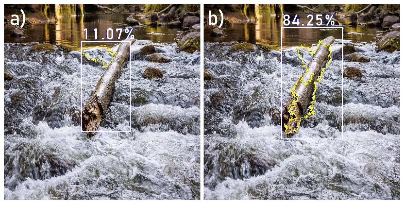
Figure 8 Wood detections according to the models trained with the (a) baseline scenario and (b) scenario 9 (“Added (V1)”), where labelled close-up images of non-submerged wood were added. The heaviest-weighted pixels, as determined by the neural networks, are indicated in yellow. Image source: http://dreamstime.com (last access: 1 March 2024).

4.4 Alternative neural networks for wood detection

While neural networks like R-CNNs, the SSD, and CenterNet offer potential for wood detection, each has its limitations for our specific application. The two-step process of R-CNNs results in longer processing times, making them less suitable for real-time detection tasks. The SSD can struggle with objects of varying sizes or those partially occluded, common in river environments. Similarly, CenterNet's key-point detection approach may not handle the complex and dynamic nature of floating wood as effectively. In contrast, the YOLO algorithm's single-stage detection, with its speed and ability to handle diverse scenarios in real time, makes it a more practical and efficient choice for automating floating-wood detection across various riverine conditions. However, it is important to note that we have not tested these models directly in our study, so their performance in this specific context remains speculative and is based on the general limitations reported in the literature.

4.5 Limitations of using low-cost cameras

Though low-cost cameras can aid research by offering economical means of capturing data, their use in detecting instream wood poses some limitations. Firstly, the lens and sensor quality of budget-friendly cameras often falls short compared to higher-end models, leading to less-detailed images (Taylor et al., 2023). This lack of detail can make it even harder to distinguish small pieces of wood from noise within the frame (Casado-García et al., 2022). Additionally, lighting conditions are generally handled less effectively, and glare from the water surface can obscure the visibility of wood. Lastly, in the absence of an International Protection Rating certification, the lower durability of budget cameras in outdoor environments can lead to malfunctions and, consequently, gaps in the data. However, the benefits of data being widely available do make low-cost cameras a valuable and accessible source of data.

5 Conclusions

We trained a convolutional neural network to detect instream wood, achieving a weighted average performance with a mean average precision (mAP) of 67 %. On the best occasion, the model had a mAP of 93 % for one specific dataset. The performance was sensitive to the quality of the images in the training data, as evidenced by a wide range of the results. For an unseen test dataset, the model's mAP performance was 61 %, in line with the results from the sensitivity tests. Efforts to improve the model's performance were, in some cases, successful. Depending on the data that were used for training, the model's performance increased by up to 23 % (mAP). Changing the sampling strategy by adding or removing training data yielded considerable differences in average performance. Additionally, although enhancing the image input resolution increased the processing time and made the method more costly, in some instances, it resulted in an increase in mAP of almost 20 percentage points. On the other hand, data augmentation and different sampling methods did not seem to greatly influence the model's performance.

Even though efforts were made to create a training database with various examples, the training results still indicated that the model overfitted the training data. Still, this study demonstrates that the model can generalize the concept of wood, especially when the training data consist of high-definition photos of labelled wood samples. Additionally, and more fitting to the general applicability of the method, we show that it can also generalize the concept of wood in rivers when the samples have different (smaller) dimensions. Large samples of wood (around 500×500 pixels) were in the database and were notably different in size compared to the smaller samples (around 10×10 pixels). When training a custom model, it is advisable to analyse the data that need to be analysed and pick the datasets from our database accordingly. For this, it is crucial to use the training datasets that resemble these data. A labelled training database of over 15 000 images was created in the research process. The training data are hosted publicly and can be used for future object detection refinements. Additionally, as the data are separated based on location and date, a customized model can be trained using the data that most closely represent the data used by the person interested. For a new wood detection study, custom-labelled data can be added to the training database to increase the performance even more. This has been emphasized as tests demonstrated that adding just 176 labelled images from the same monitoring station (but collected on a different day) could increase the model's performance by 19 percentage points.

Despite its potential, the proposed method cannot yet be used in real time. In future efforts, smaller versions of the evaluated models, such as the tiny version of the YOLO model, could be developed to run on in-field or mobile devices. In certain instances, merging three subsequent frames improved results, suggesting that incorporating temporal imaging and the time component of a video could enhance the model's performance in detection tasks. Lastly, newly labelled datasets for custom models could be added to the larger database to aid in developing the performance of the model.

5.1 Recommendations for the future development of (custom) wood-detecting CNNs

1. Tailor training data to target conditions. For the best results, use training datasets that resemble the intended deployment environment. For example, matching image quality, wood size, and contextual characteristics between training data and target conditions can improve performance.

2. Prioritize high-definition image samples. Using high-resolution images can improve the model’s generalization to the concept of wood, though this approach requires a balance with computational costs.

3. Expand training with custom-labelled data. Incorporating additional labelled data, especially data specific to the deployment site and context, can significantly improve model performance. For example, adding even a small set of labelled images from similar locations or conditions has been shown to enhance results.

4. Consider sampling strategies. Adjusting sampling strategies (such as by including larger or smaller amounts of training data) can impact the average performance. Evaluate the trade-offs between model performance and data quantity when assembling training datasets.

5. Investigate temporal-data integration. Integrating information from consecutive video frames may improve detection by capturing movement patterns. This could be particularly relevant for video-based wood detection.

6. Optimize for real-time applications. For real-time detection, consider experimenting with smaller model architectures, such as Tiny-YOLO, to reduce processing requirements for in-field or mobile device applications.

Appendix A: Training data analysis

A1 Principal component analysis

The PCA revealed a silhouette score of 0.034 with six clusters when using all 6400 dimensions of the cropped-out bounding boxes, rescaled to a resolution of 80×80 pixels. This low silhouette score from the PCA suggests that our data are very diverse. In theory, this is advantageous as it suggests the potential for training models to detect wood under varying conditions. However, distinguishing between wood detection and the detection of less-defined shapes depends heavily on the quality of the data used. The performance of a detection algorithm when detecting small samples can be compromised by including high-definition wood images, while the performance of a wood detection model can be impaired by incorporating datasets with small samples. Therefore, it is crucial to define the specific application of the model and develop a tailored approach accordingly.

Figure A1 shows the results of the k-means analysis. The fourth graph (Fig. A1d) partitions the data into eight clusters. One specific cluster exhibits a high silhouette score, suggesting a high degree of similarity among the images within this cluster. Despite efforts to eliminate duplicates, further examination of the data revealed that these images represent the same log, positioned identically across successive frames. In future experiments, it would be advisable to remove the redundant instances in this cluster from the training dataset to enhance the model's performance.

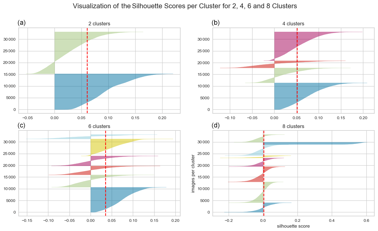
Figure A1 Visualization of a k-means analysis using two clusters with a silhouette score of 0.061 (a), four clusters with a silhouette score of 0.052 (b), six clusters with a silhouette score of 0.035 (c), and eight clusters with a silhouette score of 0.005 (d).

A2 Data diversity

Figure A2 presents a visualization of the data diversity using t-distributed stochastic neighbour embedding (t-SNE), a dimensionality reduction technique primarily employed for visualization purposes. The 20 known datasets are represented as distinct clusters, with each example indicated by its cluster's colour. While the absolute distances between the examples in the figure are not meaningful, the method clusters similar neighbours closer together. The visualization demonstrates that, in general, the samples are well distributed. The overlap between clusters accounts for the low silhouette score, indicating high variability within the data. However, small, concentrated groups of images outside the central cluster can be identified as duplicates in the training data. To address this, the data-trimming step aims to reduce the influence of these sub-clusters. This will prevent the final model from being disproportionately rewarded for correctly detecting a specific piece of wood, thus mitigating the risk of overfitting.

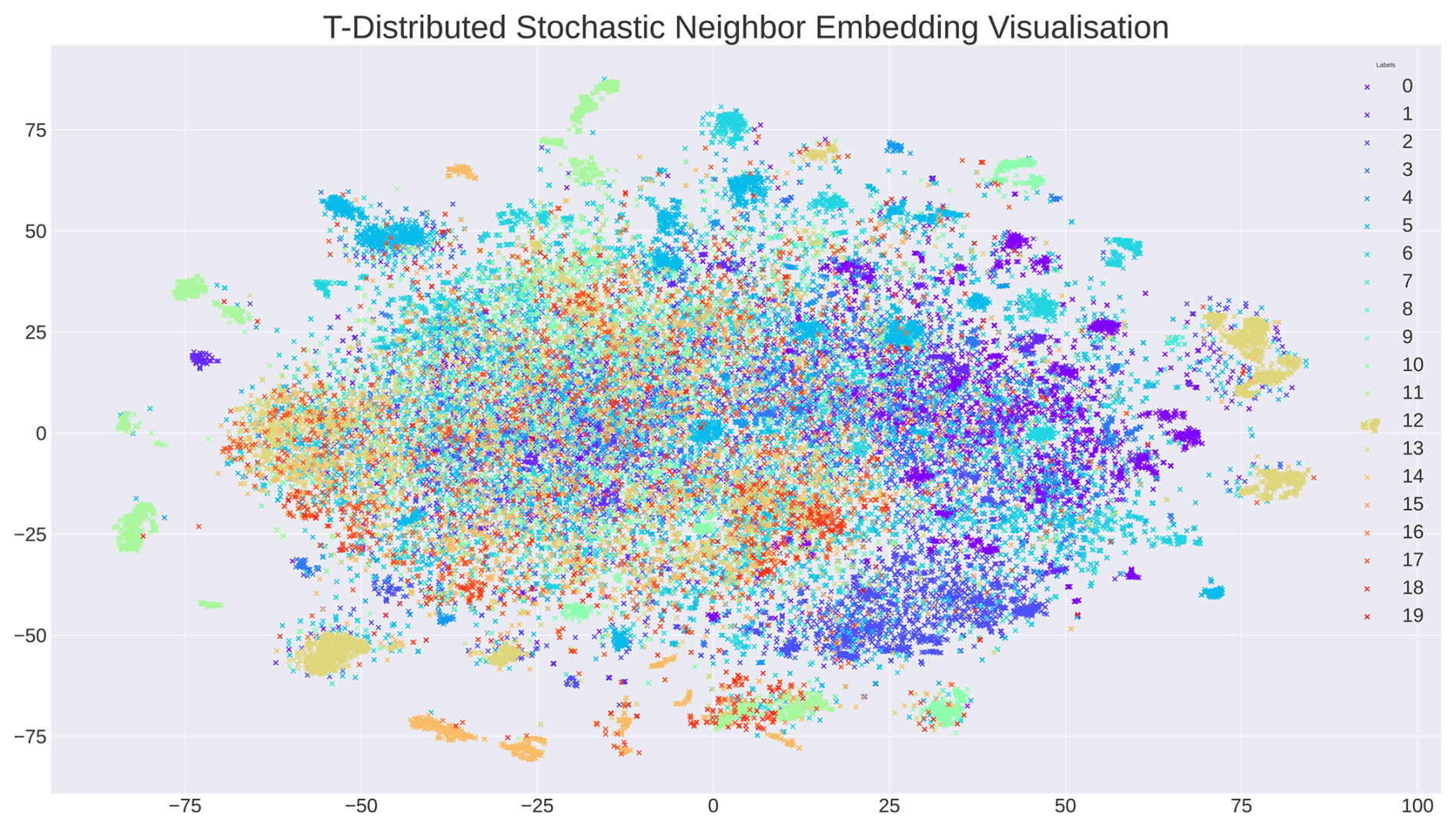
Figure A2 Clustering visualized using t-distributed stochastic neighbour embedding (van der Maaten and Hinton, 2008), resulting in a visualization of all 33 000 samples. The different colours represent the 20 different datasets. Distinctive clusters in the figure primarily share the same colour and are, therefore, part of the same dataset.

Appendix B: Dataset acquisition example

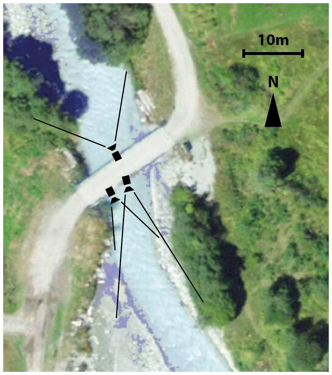
A variety of camera-mounting techniques were employed to capture videos of floating wood, including securing mobile phones with duct tape for stability in challenging outdoor environments. This allowed for flexible and accessible monitoring from bridges and stationary structures (see Fig. B1). Figure B2 shows an example of the camera positioning at the Borgne d'Arolla. Cameras were mounted to observe the river from different angles.

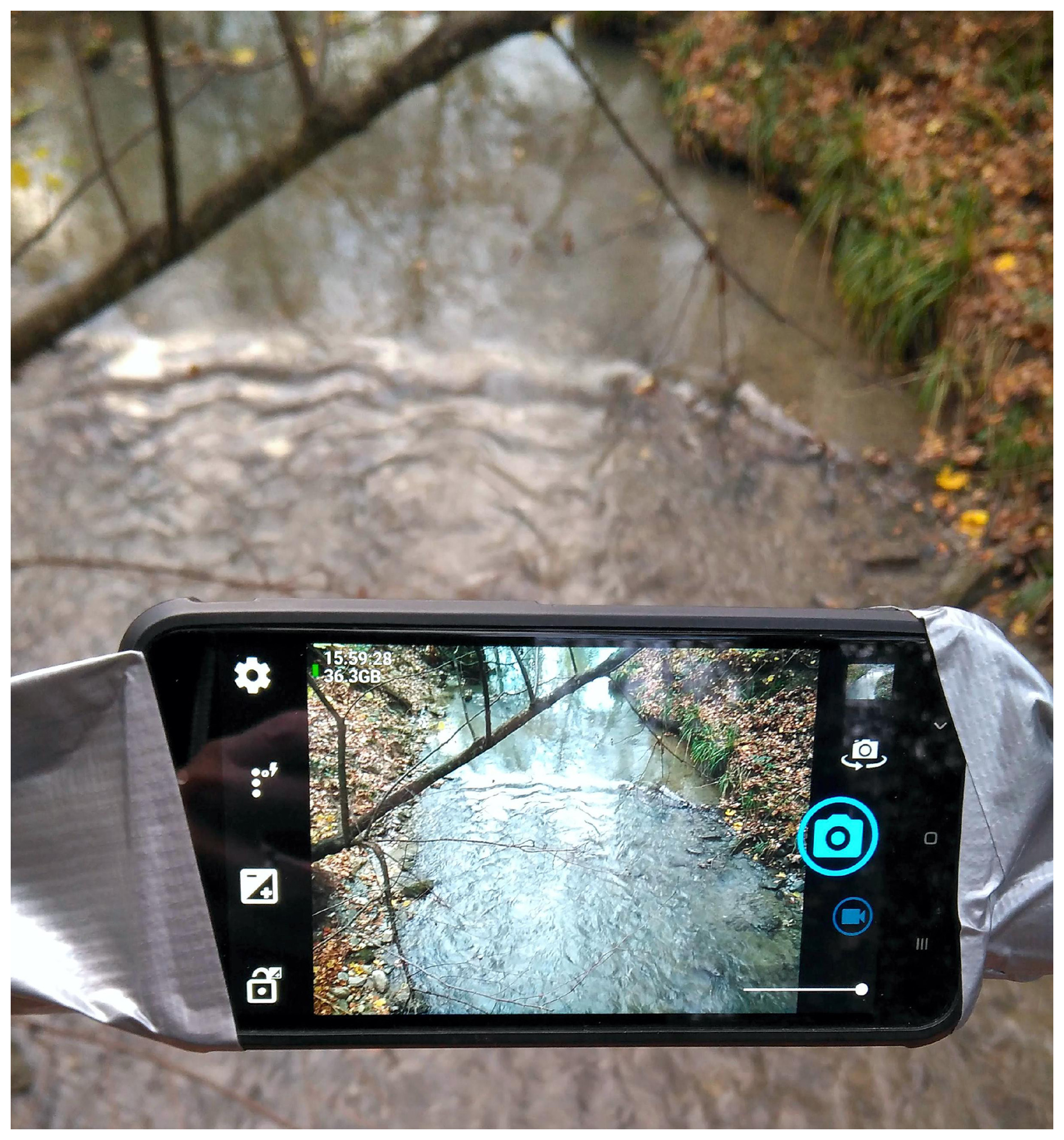
Figure B1 Example image of the data acquisition (dataset 5). A mobile phone camera was securely mounted with duct tape, providing a stable view of the river's surface from a bridge.

Figure B2 Example of the setup of the cameras on a bridge over the Borgne d'Arolla.

Appendix C: Dataset examples

Figures C1 and C2 show examples of bounding boxes from datasets 1 and 12. The samples from dataset 12 are small and, therefore, have been cropped and enlarged by 500 %.

Figure C1 Example image (dataset 1). The bounding boxes have been cropped without being resized.

Figure C2 Example image (dataset 12). The bounding boxes have been cropped and uniformly enlarged by 500 %.