Investigating uncertainty and parameter sensitivity in bedform analysis by using a Monte Carlo approach

Precise and reliable information about bedforms regarding geometry and dynamics is relevant for many applications – such as ensuring safe conditions for navigation along the waterways, parameterizing the roughness of the riverbed in numerical models, or improving bedload measurement and monitoring techniques. There are many bedform analysis tools to extract this information from bathymetrical data. However, most of these tools require the setting of various input parameters, for which specific values have to be selected. How these settings influence the resulting bedform characteristics has not yet been comprehensively investigated. We therefore developed a workflow to quantify this influence by performing a Monte Carlo simulation. By repeating the calculations many times with varying input parameter settings, the possible range of results is revealed, and thus the procedure-specific uncertainties can be quantified. We implemented a combination of the widely used zero-crossing procedure to determine bedform geometries and a cross-correlation analysis to determine bedform dynamics. Both methods are well known and established, which ensures the transferability and value of the findings. In order to increase the robustness of the workflow, we implemented a wavelet analysis based on Bedforms-ATM (Guitierrez et al., 2018), which is carried out before the zero-crossing procedure. This provides further orientation and accuracy by identifying predominant bedform lengths in a given bed elevation profile. The workflow has a high degree of automation, which allows the processing of large amounts of data. We applied the workflow to a test dataset from the Lower Rhine in Germany that was collected by the German Federal Waterways and Shipping Administration in February 2020. We found that bedform parameters reacted with different sensitivity to varying input parameter settings. Uncertainties of up to 35 % and up to 50 % were identified for bedform heights and bedform lengths, respectively. The setting of a window size in the zero-crossing procedure (especially for the superimposed small-scale bedforms in cases where they are present) was identified to be the most decisive input parameter. Here, however, the wavelet analysis offers orientation by providing a range of plausible input window sizes, and it thus allows for a reduction in uncertainty. Concurrently, the time difference between two successive measurements has been proven to have a significant influence on the determination of bedform dynamics. For the test dataset, the faster-migrating small-scale bedforms were no longer traceable for intervals longer than 2 h. At the same time, they contributed to up to 90 % of the total bedload transport, highlighting the need for measurements at high temporal resolution in order to avoid a severe underestimation.

1 Introduction

Bedforms are ubiquitous in rivers with sandy or gravelly beds (Carling et al., 2006; Kleinhans, 2001; Van Rijn, 1993). Their occurrence, shape, dimensions and dynamics depend on hydraulic and morphological conditions. Knowing bedforms is crucial for various fields of application. For example, bedform crest heights influence the navigable depth along the waterways (e.g., Carling et al., 2006; Scheiber et al., 2021). This is why information about maximum bedform heights is required in order to ensure safety and ease of navigation. From the perspective of hydraulics, bedforms increase the flow resistance at the riverbed. In numerical modeling, bedform dimensions and shapes often need to be parameterized and transformed into form roughness (Lefebvre and Winter, 2016; Venditti, 2013). The erosion of particles on the bedforms' upstream faces and the accumulation on their downstream faces result in a downstream movement of sediments, contributing to bedload transport (Simons et al., 1965). Therefore, bedload transport rates can be estimated based on bedform migration – so-called dune tracking (e.g., Claude et al., 2012; Leary and Buscombe, 2020; Simons et al., 1965) – representing an alternative approach to direct bedload measurements.

Over the years many tools were developed to derive both bedform geometries and migration rates from multibeam echo sounding (MBES) data (e.g., Cisneros et al., 2020; Gilja et al., 2013; Guitierrez et al., 2018; Henning, 2013; Lee et al., 2021; Lebrec et al., 2022; Lefebvre et al., 2022; Núñez-González et al., 2021; Ogor, 2018; Scheiber et al., 2021; Van der Mark and Blom, 2007; Van Dijk et al., 2008; Wang et al., 2020; Zomer et al., 2022). Most of these tools require the setting of procedure-specific input parameters. There are often no theoretically sound criteria or anything like best practice for setting a specific value. For example, a widely used and established approach is the zero-crossing procedure, which is implemented in many published tools and has been used in many studies (e.g., Van der Mark and Blom, 2007; Leary and Buscombe, 2019; Wang et al., 2020; Zomer et al., 2022). The identification of bedforms crests and troughs in a longitudinal bed elevation profile (BEP) is based on the calculation of a moving average, which requires the setting of a window size. However, there are no equations or guidelines for choosing a specific value. Therefore, the procedure is strongly influenced by the personal experience and subjective selection of the investigator. If applied by several investigators, different results will be obtained from the same procedure and for the same dataset. Despite the ubiquitous need to define the setting of these parameters, little attention has been paid to how different settings influence estimated bedform characteristics. A Monte Carlo simulation (MCS) is a suitable approach to evaluate this influence of input parameter settings. An MCS is a computer-based analytical method that utilizes sequences of random numbers as inputs into a model in order to obtain a probabilistic approximation to the solution (Adekitan, 2014). With regard to bedform analysis, repeated calculations with varying input parameter settings reveal the possible range of results and enable robust estimates of the resulting bedform characteristics.

We therefore developed a workflow to perform extensive sensitivity and uncertainty analyses and applied it to a field dataset. The workflow includes an initial wavelet analysis, a zero-crossing procedure to determine bedform geometries and two different approaches to analyze bedform dynamics, which are partly based on existing tools. These individual steps are embedded in an MCS routine to repeat the calculations with varying input parameter definitions. This is the key feature of the workflow and allows us to quantify the range of uncertainty for different bedform parameters (e.g.,  height, length and migration rate) due to the input parameter settings. It also allows us to compare the sensitivity of the different input parameters further down the line. Both will be of great value for future studies when estimating the uncertainty and the robustness of produced results.

There are essentially two key research questions for this study. First, what is the sensitivity of the individual input parameters? Second, what is the total level of uncertainty to be expected due to varying input parameter settings? In order to adequately address these research questions, the following aspects were decisive for the development of the workflow.

• Automation. Due to increasing data availability and the need for repeated calculations (within the MCS), it was essential to achieve a high degree of automation to enable batch processing of large datasets. Therefore, the algorithm was coded in a way that allows for easy selection of multiple datasets and the performance of many iterations.

• Transferability and value. As mentioned earlier, there are lots of different bedform analysis tools available. Each of them is complex and it would be beyond the scope of this work to combine them within one comprehensive study. Therefore, we selected the well-established zero-crossing procedure to determine bedform geometries in combination with the cross-correlation analysis to determine bedform dynamics. Both approaches have been used in many studies or are even implemented in recently published tools (see the list above). In this way, the value and transferability of the findings for future research can be increased. With regard to bedform dynamics, we use the zero-crossing procedure in combination with a newly introduced method as a second approach, which allows for further validation and provides new insights into bedform dynamics.

• Robustness. Before the MCS can be carried out, a value range must be specified within which the input parameters are varied. In order to provide orientation and thus avoid diverging results, a wavelet analysis was added to the workflow based on Bedforms-ATM (Guitierrez et al., 2018). This allows for initial estimates about prevailing bedform lengths in a given BEP, which are required input parameters for the zero-crossing procedure. In this way, the boundary conditions for the MCS can be defined and the accuracy and the robustness of the procedure increased. The combination of wavelet analysis and zero-crossing procedure has already proven to be efficient in the algorithm developed by Wang el al. (2020). A further aim was to increase the robustness of the statistical evaluation of bedform characteristics. We therefore introduce a new parameter as a measure of total bedform height, which behaves more robustly compared to existing measures.

The entire workflow is based on the evaluation of longitudinal BEPs. Due to the high degree of automation, large numbers of BEPs can be analyzed. By using a dense arrangement of the individual BEPs and analyzing different angles, a 3D analysis could be approximated. We applied the workflow to a test dataset that contains MBES data of a 500 m stretch of the Lower Rhine in Germany. The data were collected during a 3 d campaign in February 2020 by the German Federal Waterways and Shipping Administration.

Section 2 introduces the implemented workflow and contains detailed descriptions of the individual steps and implemented methods. This is followed by a description of the MBES dataset from the Lower Rhine. In Sect. 4, the resulting bedform parameters and bedload transport rates are presented. Section 5 focuses on the interpretation of the results and the sensitivity of the different procedure-specific input parameters. Finally, the key findings are outlined in Sect. 6.

2 Method

Before describing the individual steps of the implemented workflow in detail, Fig. 1 provides an overview for orientation. The workflow consists of the following key points.

• Input data. These data consist of longitudinal BEPs derived from MBES data.

• Step 1 – wavelet analysis. In this step, predominant bedform lengths are identified in a given BEP by a continuous wavelet transform based on Bedforms ATM. These are required input parameters for step 2.

• Step 2 – zero-crossing procedure. This step requires the identified predominant bedform lengths as input parameters (window sizes) for the zero-crossing procedure, based on the software RhenoBT (Frings et al., 2012), in order to determine bedform geometries. By extending the original algorithm, a data export of tables containing information about individual bedform attributes (e.g., height, length and shape) was implemented to enable extensive statistical analyses as an optional post-processing routine. In addition, new statistical parameters for the characterization of bedform geometries were defined.

• Step 3 – cross-correlation/centroid analysis. This step consists of the calculation of bedform migration rates based on determined bedform geometries using a cross-correlation analysis or a newly introduced centroid analysis that detects the migration of the geometrical centroids of individual bedform areas. Bedload transport rates can be derived from a known migration rate by considering grain density and porosity.

• MCS. The setting of input parameters is required at various points in the workflow. This has an impact on the results that is not immediately apparent to the user. Therefore, the calculations are repeated multiple times with different input parameter settings in order to reveal the range of plausible results and to evaluate the level of uncertainty.

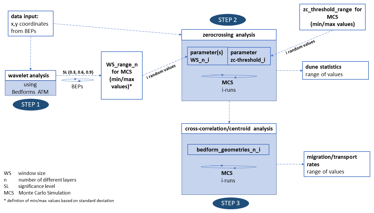
Figure 1 The implemented workflow consists of three steps. Parts of the workflow are performed as an MCS to consider the uncertainties associated with the setting of various input parameters.

2.1 Preprocessing and data preparation

Before the actual analysis, the spatial discretization of the river section under investigation has to be defined. Spatial discretization lateral to the flow direction is given by the distance between the BEPs. The more heterogeneous the investigated bedform field is (high spatial variation in bedform dimensions), the denser the arrangement of BEPs should be. In the longitudinal direction, a division into sections is mandatory. The statistical parameters (e.g., the average bedform height and length) are calculated per section (see Sect. 2.4).

In order to obtain the BEPs from the MBES data, some hydrographic preprocessing steps are required. Based on the plausibilized raw MBES data, geometric modeling is suitable to reduce included measurement uncertainties. For this purpose, the measurement data are gridded, and for each grid point a polynomial is approximated to the 3D point cloud within a given radius. In the case of the test dataset from the Lower Rhine, a surface approximation with polynomials using a least-squares fit was applied. Along the considered profile tracks, the individual BEPs are derived from the DEMs. A detailed description of hydrographic preprocessing steps can be found, e.g., in Lorenz et al. (2021).

2.2 Wavelet analysis

The first step of the workflow is a continuous wavelet transform based on Bedforms-ATM. It is performed to identify the predominant wavelengths (interpreted as bedform lengths) in the individual BEPs. The predominant bedform lengths are required input parameters for the zero-crossing procedure that follows in the second step. Wavelet transforms have been used in a variety of applications to analyze riverbed roughness (Nyander et al., 2003) or to discriminate engineering surfaces (Raja et al., 2002). They are more suitable for signals containing discontinuities compared to Fourier methods. In terms of bedform analyses, the so-called Morlet wavelet appears to be the most efficient (Guitierrez et al., 2018) and has been used for all analyses in this study. As a result of the wavelet transform, a spectrum is obtained that indicates the dominance of individual wavelengths in a BEP. Figure 2 shows the so-called wavelet power spectrum for an exemplary BEP excerpt. Based on the chosen significance level, the predominant wavelengths are identified. Only those peaks in the wavelet power spectrum that are greater than the global significance level are considered. By default, the significance level has to be set by the user. In the shown example (Fig. 2), three different significance levels lead to three different results. The workflow has been adapted accordingly, meaning that the analysis is executed three times for each BEP with significance levels of 0.3, 0.6 and 0.9, respectively. If two predominant wavelengths (equal to two individual peaks included in the wavelet power spectrum) are detected, it is assumed that two coexistent layers of bedforms are present. For example, small-scale secondary bedforms might be migrating over large-scale underlying bedforms with (likely) higher migration rates (e.g., Carling et al., 2006; Gilja et al., 2013; Kleinhans et al., 2002).

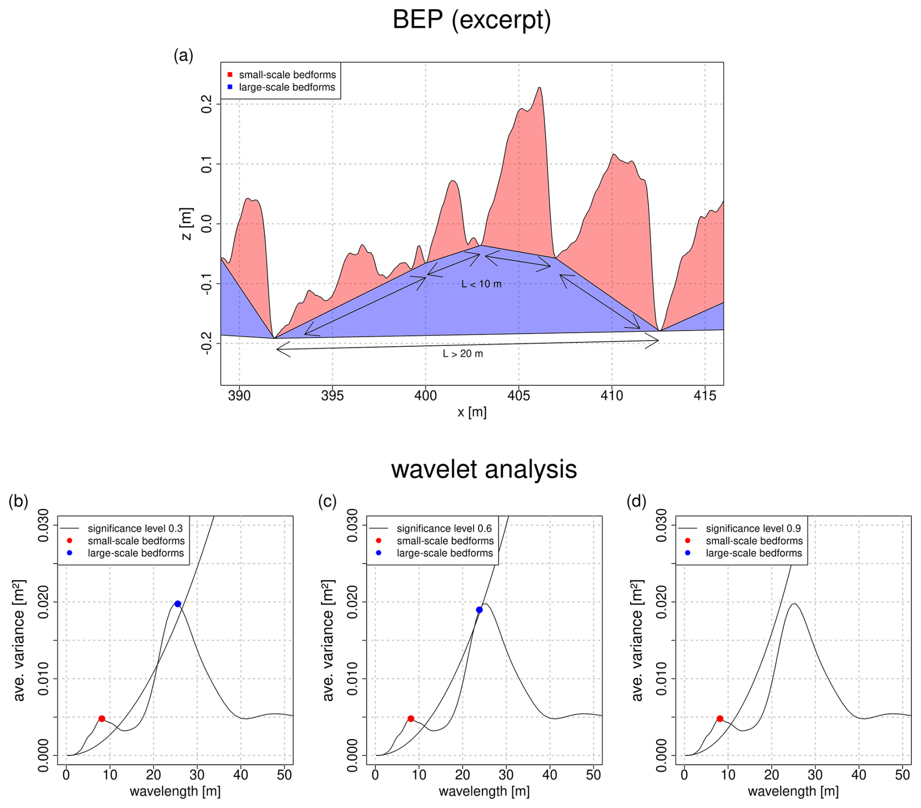
Figure 2 Here we identify predominant wavelengths of a BEP using wavelet analysis. Different wavelengths are identified depending on the chosen significance level. (a) Excerpt of an exemplary BEP of the test dataset from the Lower Rhine separated into two layers of bedforms. (b–d) Identified predominant wavelengths using wavelet analysis with a significance level of 0.3, 0.6 and 0.9, respectively. In the first two cases (b, c) two layers of bedforms are identified. In the third case (d) only one layer of bedforms is identified.

The resulting wavelengths from all analyzed BEPs are stored in a table. This table contains the total number of detected wavelengths and is passed to the next step in the workflow (zero-crossing procedure) after outliers have been removed. For this purpose, the mean value and standard deviation σ are calculated for each detected bedform layer. Values that lie outside the range of ±2σ around the mean value are removed. Nevertheless – before carrying out the further calculation steps – it is recommended to check the results from the wavelet analysis for plausibility, to compare them with site-specific knowledge about occurring bedform dimensions and to make manual adjustments if necessary. The most sensitive step is deciding on the number of bedform layers representing features with predominant wavelengths. Due to potential ambiguity of the results, this step is not automated but requires a critical assessment based on the present morphological conditions. In the example shown in Fig. 2, different significance levels indicate a different number of bedform layers for the same BEP. In the first case (Fig. 2b), two bedform layers are detected with wavelengths of 8 m and 26 m. In the second case (Fig. 2c), two bedform layers are detected with wavelengths of 8 and 23 m. In the third case (Fig. 2d), only one layer with a wavelength of 8 m is detected because the second peak is below the global significance. This decision has a great impact on all analyses that follow (in a recently published meta-analysis by Scheiber et al., 2024, in which five bedform analysis algorithms were compared, the consideration of a second bedform layer was also identified as the most significant cause of deviations between the results of the different algorithms). For instance, the estimated bedload transport rates at the end of the procedure can be overestimated or underestimated based on the selected number of bedform layers. To make this decision, a visual inspection of the BEPs is recommended. In addition, the calculation of bedform migration rates can be used as validation. If migration rates with high correlation coefficients can be detected for both bedform layers, it can be assumed that the number of layers has been chosen correctly.

Optionally – especially in case of larger-scale gradients of the channel bed (e.g., due to underlying bars) – a detrending of the BEPs can be performed using robust spline filter techniques. The algorithm is based on a discrete cosine transform and is used to smooth the initial signal. The degree of smoothing depends on the adjustable s parameter (for further information, refer to Gutierrez et al., 2013).

2.3 Zero-crossing procedure

The zero-crossing procedure is adapted from the software RhenoBT that, in turn, is based on the bedform tracking tool created by Van der Mark and Blom (2007). It is a widely used approach for analyzing BEPs with respect to bedform geometries (see Sect. 1). Here a moving average is calculated over the considered BEP by setting a window size. The chosen window size should ideally approximately correspond to the expected bedform length. For this reason, the results from step 1 (wavelet analysis) provide the rationale for setting the adequate window size. The zero crossings are calculated based on the moving average. The local minima between each two zero crossings are interpreted as bedform troughs. To limit the effect of small-scale fluctuations in the BEPs a zero-crossing threshold (hereafter referred to as zc threshold) is used to define the minimum distance between a bedform trough and the moving average. Only local minima with distances larger than the zc threshold are considered. There are no objective criteria for its exact definition, but globally it must not be greater than the minimum expected bedform height. At the end of the procedure, one or two (depending on the selected number of bedform layers) baselines are constructed that separate the individual bedform layers from each other. The lowest baseline separates the bedforms from the non-active layer of the riverbed. The individual bedform attributes (height, length and shape) are calculated based on this separation. If two bedform layers are present, the individual attributes are calculated for each layer separately. In such a case the baseline of the small-scale bedforms is calculated first. Following this, the procedure is repeated by calculating the moving average – with the corresponding window size for the underlying large-scale bedforms – over the previously calculated baseline of the small-scale bedforms. The procedure is illustrated in Fig. A1.

2.4 Bedform statistics

The results of the zero-crossing procedure can be exported as tables, which summarize geometric attributes for each individual bedform and the chosen input parameter settings (Table 1), e.g., to enable subsequent statistical analyses as a post-processing routine. The tables are exported for each BEP, section, bedform layer and iteration of the MCS.

Table 1 Output from the analysis containing geometrical attributes for each bedform layer.

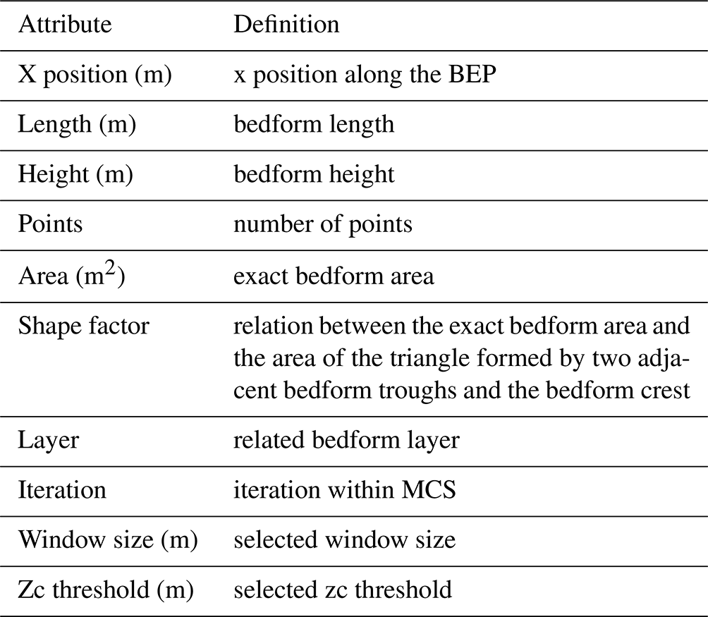
In accordance to the definition of individual attributes described in Wesseling and Wilbers (2000), bedform length is defined as the length of the line connecting two adjacent troughs, while bedform height is the height of the triangle formed by a crest and its two adjacent troughs. Total height H_total is determined by measuring the height of the triangle, which is defined by two adjacent troughs of the large-scale bedforms and the maximum of the BEP in between (see Fig. 3a). Total length L_total is equal to the length of the large-scale bedforms. The shape factor S (–) is the relation between the exact bedform area and the simplified bedform area resulting from the triangle formed by bedform height and length (Ten Brinke et al., 1999).

$$\begin{array}{}\text{(1)}& S={\displaystyle \frac{A}{\mathrm{0.5}\cdot H\cdot L}}\end{array}$$

Based on these individual bedform attributes, statistical parameters are calculated to describe average bedform characteristics in a defined section of the BEP. For this purpose, the median is formed over all individual bedform attributes contained in a section. Since the determination of these parameters results from the averaging of individual attributes, their significance depends on the number of detected bedforms in the considered section. For this reason, another parameter for estimating the total bedform height was implemented that is independent of the number of identified bedforms. For obtaining the so-called T₉₀ parameter, in each x value the vertical difference between lowest baseline and the BEP is calculated (see Fig. 3b). Finally, the 90th percentile of the resulting values is formed within each section. The parameter is therefore not based on measuring the height of individual bedforms but on measuring the accumulated bedform layer thickness (T) along the entire BEP. The 90th percentile approximately corresponds to the average total bedform height of individual bedforms in a section. This means that both T₉₀ and H_total are used to quantify the same property, but T₉₀ is expected to behave more robust due to the mentioned aspects. Definitions of all parameters are given in Table A1.

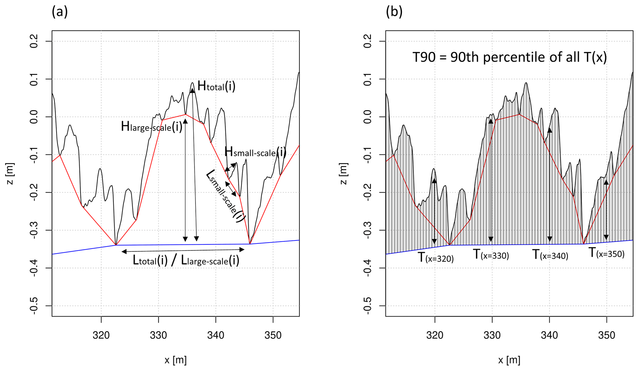
Figure 3 (a) Definition of individual bedform attributes. (b) Determination of the T₉₀ parameter.

2.5 Estimation of bedform migration and bedload transport

Bedform migration rates can be determined if consecutive measurements over time are available. For this purpose, two different methods were implemented. The first method is a cross-correlation analysis that identifies the spatial offset between two consecutive BEPs (Leary and Buscombe, 2019; McElroy and Mohrig, 2009; Van der Mark and Blom, 2007). Migration rates are determined using the known time difference between each set of two measurements. They can be estimated for the total BEP and for the individual bedform layers by using the constructed baselines from the zero-crossing procedure. This can be a decisive aspect in cases where bedforms of different dimensions occur that migrate with different rates. As many different solutions emerge from the MCS for constructing the baselines (because different input parameter settings are used), the cross-correlation analysis is also carried out as an MCS. Therefore, many iterations are performed with different baselines for the same BEP. To consider the small-scale bedforms of the upper layer separately, the upper baseline is subtracted from the initial BEP. The resulting geometries represent the isolated small-scale bedforms and are subsequently used in the cross-correlation analysis. To consider the large-scale bedforms of the lower layer, there are two possible approaches that were evaluated before the final implementation. The first approach is based on a subtraction of the lower baseline from the upper baseline. However, preliminary results (not shown here) indicate that correlations are relatively low for this approach. Another option is to directly use the upper baseline in the cross-correlation analysis. Both approaches lead to an isolated representation of the large-scale bedforms. The second approach proved to be more suitable, as higher correlations could be achieved, and therefore this approach was implemented.

In addition to the cross-correlation analysis, an alternative method has been developed to better determine the migration rates of the small-scale bedforms. The migration of smaller superimposed bedforms decisively contributes to total bedload transport. The resulting quantity may even exceed the transport associated with larger underlying bedforms (Zomer et al., 2021). This highlights the need for a more detailed analysis of this process. In the presented method, individual migration rates are obtained – instead of an average migration rate along the entire BEP – by tracking the geometric centroids of individual bedform areas. Geometric centroids are calculated for all individual bedform areas obtained from the zero-crossing procedure for two consecutive measurements. Each centroid from the first measurement is assigned to the centroid from the second measurement with the smallest distance in downstream direction. The offset between each pair of centroids corresponds to the individual migration distance. By knowing the time difference between both measurements, migration rates are determined. In order to ensure a correct assignment of corresponding centroids, some plausibility check criteria have been defined. For each pair of bedforms, the ratio of bedform length ($L\left(t\mathrm{2}\right)/L\left(t\mathrm{1}\right)$) and bedform area ($A\left(t\mathrm{2}\right)/A\left(t\mathrm{1}\right)$) is calculated. To ensure a reliable assignment, a threshold allowing 25 % of deformation (concerning length and area) was set. All pairs of bedforms whose ratios exceed this threshold are excluded. This means that bedforms whose shape has already changed too much to allow for a reliable assignment are not included in the further analysis. The obtained results provide insights into the variability of bedform migration rates along a BEP and can be related to specific geometric attributes. To derive a weighted average migration rate (c_m) from the individual rates for a considered BEP, the products of individual migration rate (c_i) and corresponding bedform length (L_i) are summed up and divided by the total length of the BEP (L_BEP).

$$\begin{array}{}\text{(2)}& c_{\mathrm{m}}={\displaystyle \frac{\sum c_i\cdot L_i}{L_{\text{BEP}}}}\end{array}$$

Like the cross-correlation analysis, the centroid analysis is also carried out as an MCS by using the various bedform geometries determined in step 2.

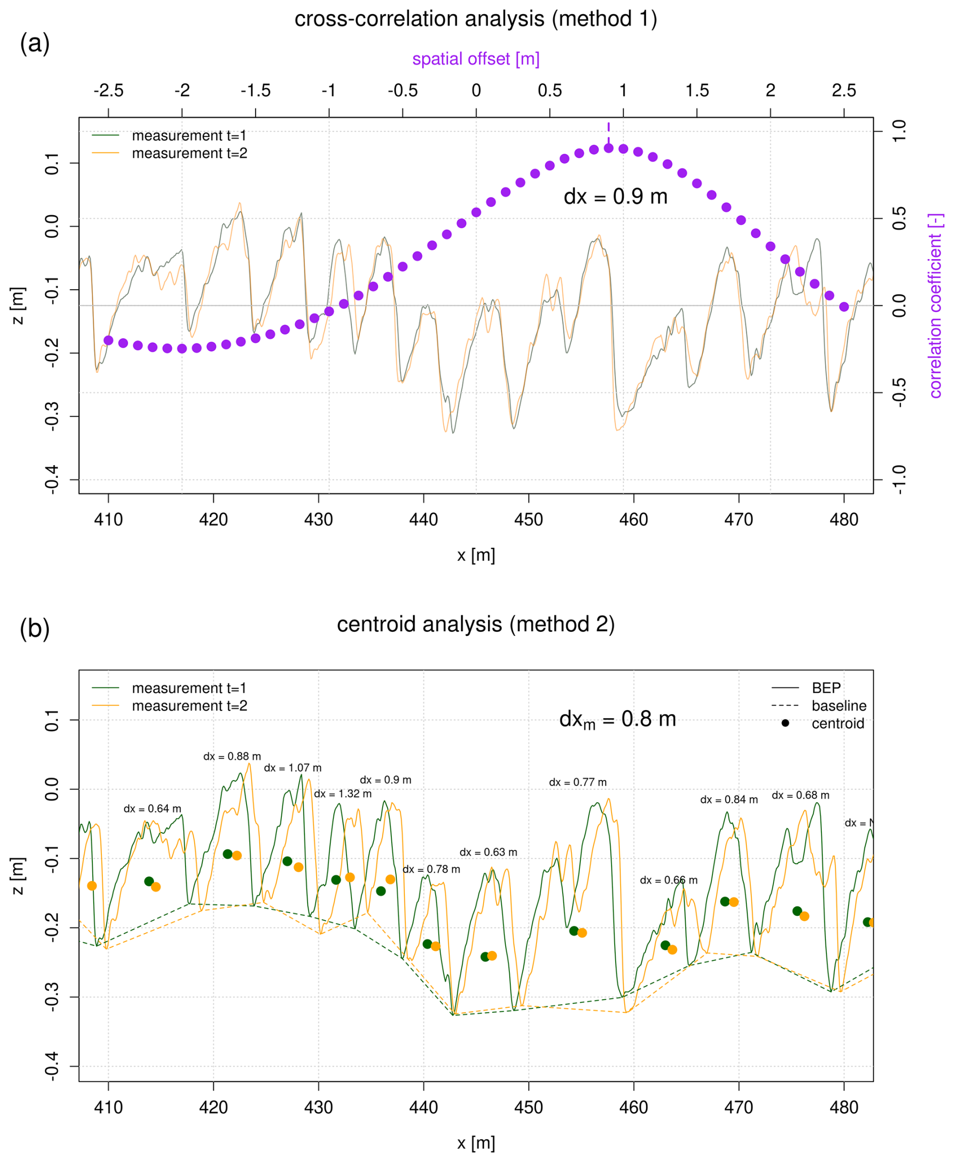
Figure 4 Calculation of bedform migration based on the cross-correlation analysis (a) and by comparing the individual bedform areas of the geometrical centroids (b). The time difference between the measurements was 0.4 h (corresponding to measurement pair no. 2 in Table A3).

Figure 4 illustrates the two methods for a pair of BEPs selected for demonstration purpose. Figure 4a shows the results from the cross-correlation analysis and the shifted BEPs. Figure 4b shows the calculated individual offsets from the centroid analysis. In the following, the cross-correlation analysis is referred to as method 1 and the centroid analysis as method 2.

Based on the obtained migration rates – and by considering porosity and density – bedload transport rates (given in $\mathrm{g}{\mathrm{s}}^{-\mathrm{1}}{\mathrm{m}}^{-\mathrm{1}}$) can be estimated. The approach by Ten Brinke et al. (1999) includes migration rate c (m s⁻¹), density ρ (g cm⁻³), porosity n (–), bedform height H (m) and shape factor S (–).

$$\begin{array}{}\text{(3)}& q_{\mathrm{b}}=c\cdot H\cdot S\cdot \mathrm{0.5}\cdot \mathit{\rho }\cdot \left(\mathrm{1}-n\right)\end{array}$$

Since during the procedure the exact area of each single bedform is calculated, shape factor and bedform height can be replaced. For this purpose, the sum A (m²) of the individual bedform areas is used. This means that no averaging of bedform characteristics along the BEP is necessary. To obtain the correct unit, the result must be divided by the total length of the BEP.

$$\begin{array}{}\text{(4)}& q_{\mathrm{b}}=c\cdot {\displaystyle \frac{A}{L_{\text{BEP}}}}\cdot \mathit{\rho }\cdot (\mathrm{1}-n)\end{array}$$

The calculation of bedload transport is also part of the MCS as the results depend on the obtained bedform geometries and migration rates.

2.6 Monte Carlo simulation

According to Fig. 1, steps 2 and 3 of the developed workflow are executed as an MCS in order to address the possible range of results and the corresponding level of uncertainty. Concerning step 1, the results of the wavelet analysis provide an orientation for setting the window sizes in step 2 (zero-crossing procedure). For each BEP, the wavelet analysis is performed three times with significance levels of 0.3, 0.6 and 0.9, respectively. The resulting bedform lengths from all analyzed BEPs are stored in a table. This table now contains the total number of detected bedform lengths. In order to exclude outliers, mean value and standard deviation σ are calculated for each layer. The final range of considered bedform lengths for each layer results from ±2σ around the mean value (denoted as “WS_range_n” in Fig. 1). These steps ensure an automated and a reproducible procedure. The obtained ranges of bedform lengths are then used in the following zero-crossing procedure.

For applying the zero-crossing procedure in step 2, the user-defined inputs are the following parameters: (i) the respective window sizes for calculating the moving average of the individual bedform layers (denoted as “WS_n_i” in Fig. 1) and (ii) the zc threshold (denoted as “zc-threshold_i” in Fig. 1). Within a given range, random values are generated for each parameter according to a uniform distribution. Concerning the window sizes, the ranges of bedform lengths resulting from the wavelet analysis are used (“WS_range_n_for MCS”). For zc threshold there is a lack of objective criteria, but globally it must not be greater than the minimum expected bedform height. The random values for (i) and (ii) are generated once and are then used for all BEPs and all repeated measurements in order to ensure comparability. Using all available sets of generated random values results in multiple representations of the bedform geometries for each BEP (denoted as “bedform_geometries_n_i” in Fig. 1). All of these representations are then used to calculate bedform migration and bedload transport rates in step 3, in which two consecutive measurements over time are always considered in pairs. To ensure comparability, only pairs of representations of the bedform geometries with identical parameter settings are considered.

By performing this MCS, the possible range of results can be quantified for all steps of the procedure. At the same time, the various statistical parameters can be examined with respect to their robustness. For examining the behavior of each input parameter separately, additional runs can be executed in which only one parameter is varied at a time while all the other parameters are kept constant. The number of iterations is freely selectable. The higher the number, the more robust the estimates. On the other hand, a very high number of iterations leads to longer computational times. With respect to the analyses shown here, 100 iterations per BEP were performed.

3 Dataset

The developed workflow was applied to an MBES dataset from the Lower Rhine in Germany. The dataset was obtained during a field measurement carried out by the German Federal Waterways and Shipping Administration in February 2020. All hydrographic processing steps (e.g., plausibility checks, geometric modeling and extraction of longitudinal BEPs from spatial data) were carried out by the German Federal Institute of Hydrology.

Figure 5 Study area near Emmerich (Rhine kilometer 860.0 to 860.5), with spatial discretization into 16 profile tracks lateral to the flow direction and 100 m sections in the longitudinal direction. The base map is from ©OpenStreetMap contributors 2023. Distributed under the Open Data Commons Open Database License (ODbL) v1.0.

The study area is located close to Emmerich at Rhine kilometer 860.0 to 860.5 and covers 500 m in length and about 200 m in width (see Fig. 5). The section is characterized by a mixed sand and gravel bed with grain sizes on the order of 6 mm (D50). According to BfG (2011), grain density was assumed to be 2.603 g cm⁻³, and for porosity a value of 0.30 was selected. The measurements were taken on consecutive days at medium- to high-flow conditions with discharges ranging from 4000 to 4200 m³ s⁻¹ at gauging station Emmerich (long-term mean discharge at 2260 m³ s⁻¹) and depth-averaged flow velocities of about 1.9 m s⁻¹ in the main channel. There was a peak in discharge 10 d before the first day of the campaign exceeding a discharge of 6000 m³ s⁻¹. The total area covered with bedforms was measured four times with intervals between 3.2 and 24 h. Additional MBES data were collected along a single measurement swath in the center of the bedform field at shorter intervals, allowing for a more detailed analysis of bedform migration and bedload transport. All measurements were collected using a Kongsberg Maritime multibeam echo sounder EM3002 combined with positioning by a Trimble antenna SPS185 in precise differential GPS mode, an estimation of the heading by a Seapath 330 system and data from an inertial measurement unit (MRU5+). Beam footprints can be quantified in the range of 0.09–0.27 m for a typical depth of 3.5 m and a beam divergence of 1.5°×1.5°. The point cloud density is about 330 points per square meter, and the measurement uncertainty regarding the elevation of a single point can be specified by 0.15 m (95 % confidence level).

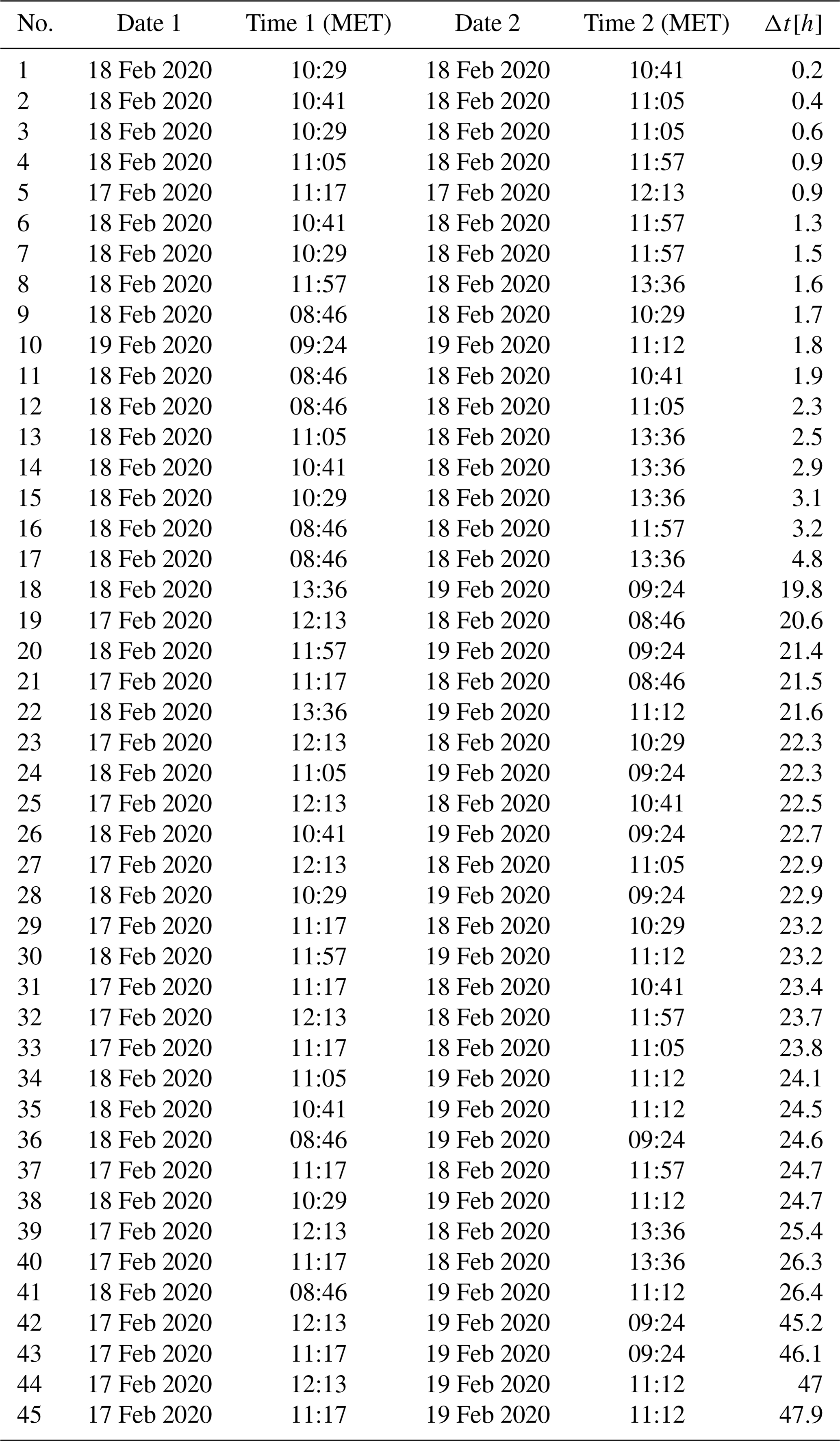
Table A2 contains all measurements performed during the campaign. In order to expand the data basis with respect to bedform migration and bedload transport, all possible combinations (for dt>0) are considered rather than only directly consecutive measurements. The 10 available detailed measurements thus result in $\left(\genfrac{}{}{0ex}{}{\mathrm{10}}{\mathrm{2}}\right)=\mathrm{45}$ possible combinations (see Table A3).

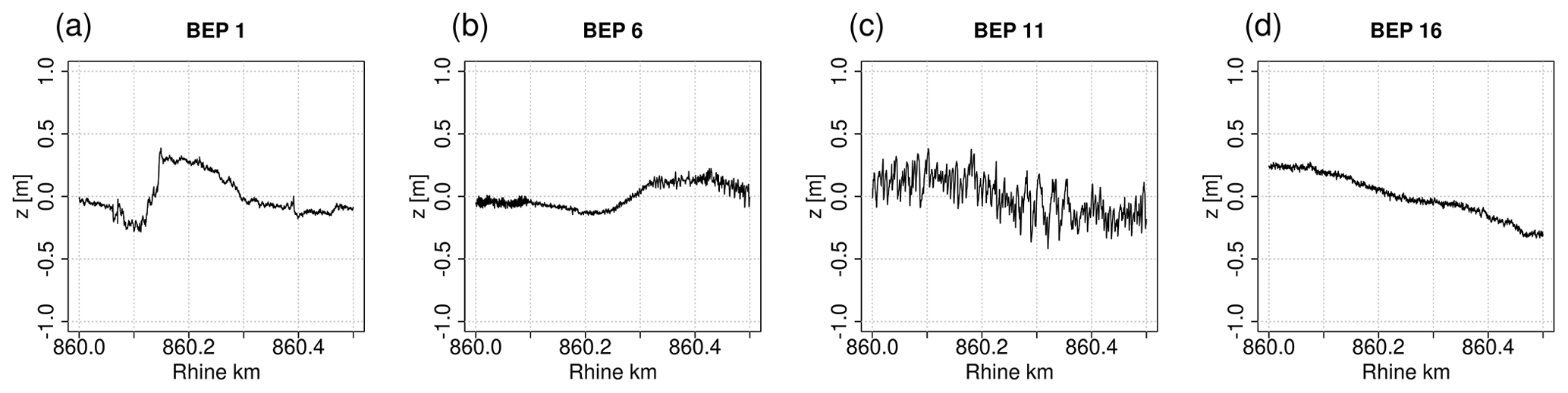
Figure 6 Selected BEPs derived from MBES data of the first measurement from 17 February 2020.

Hydrographic processing was performed according to Lorenz et al. (2021). The measurement data were plausibilized and modeled to a regular grid with a point spacing of 10 cm by a surface approximation with polynomials using a least-squares fit. Longitudinal BEPs were derived using triangular meshing of the DEM. The measured bedform field was subdivided into 16 BEPs with a lateral distance of 10 m from each other (see Fig. 5b). Starting from the left boundary of the navigation channel, the profile lines were shifted parallel as a polyline in specific intervals so that all profile lines were parallel and equidistant (10 m) from each other. Figure 6 shows some selected BEPs. All BEPs derived from MBES data from 17 February 2020 can be found in Appendix A (Fig. A2). The largest bedforms are located between BEP 8 and BEP 14, covering the entire length of the study area (see Fig. 6c). Smaller bedforms are located between BEP 3 and BEP 7, occurring only occasionally in individual sections (see Fig. 6b). Along BEP 15 and BEP 16 no significant bedforms were measured (see Fig. 6d). A macrostructure is recognizable, particularly in BEPs 1–4 (see Fig. 6a). It extends from the head of the groyne on the left bank to the middle of the channel. The length of the structure exceeds that of the other longest bedforms by an order of magnitude. When analyzing the collected MBES data, no migration of the structure could be identified within 48 h. We therefore assume that this is not a migrating bedform but an accumulation of sediments that were washed out between the groynes during the previous flood event. This is why we decided not to include it in the analyses shown in Sect. 4.2.

4 Results

4.1 Wavelet analysis

Figure 7 shows the identified predominant wavelengths calculated in the first step (wavelet analysis based on Bedforms-ATM). Wavelengths of the small-scale bedforms slightly increase from left to right, reaching a maximum of 13 m. No wavelengths could be identified near the boundaries of the study area (BEPs 1–2 and 15–16). In the center of the bedform field, a second layer of large-scale bedforms with wavelengths on the order of 25 m was detected. A visual comparison of the results with the BEPs shown in Fig. 6 confirms the plausibility of the results. The resulting migration rates from the cross-correlation analysis (see Sect. 4.3) will also verify the assumption of two separate layers. The detected wavelengths are based on all four measurements of the total bedform field and on different settings of the significance level, which were 0.3, 0.6 and 0.9, respectively. Values have been rounded to whole meters. Therefore, there are overlaps (up to 12 points per BEP and bedform scale) that cannot be recognized in the figure.

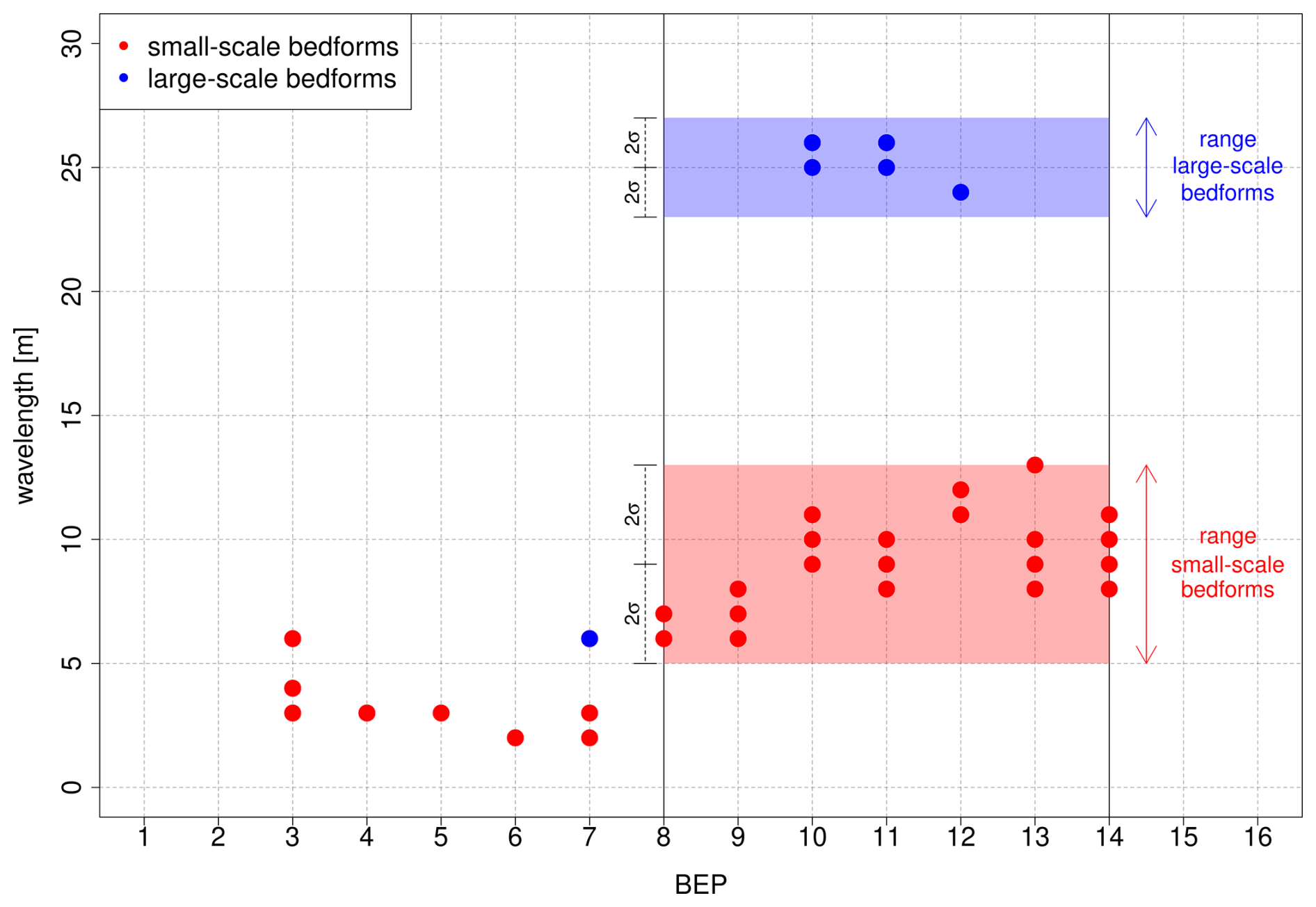
Figure 7 Derivation of the ranges of window sizes for the zero-crossing procedure from the identified predominant wavelengths in individual BEPs by means of wavelet analysis.

Only the center of the bedform field (BEPs 8 to 14) was considered in the further analyses. Along the other BEPs, either only very small bedforms occur or bedforms only cover a limited section. The ranges of respected wavelengths are defined by twice the standard deviation around the mean value (see Sect. 2.2). All detected wavelengths were within the specified ranges.

4.2 Bedform geometries

The wavelet analysis determines the range of values for the input parameter window size in the zero-crossing procedure (step 2). For each BEP, 100 iterations were performed with varying settings (MCS). Window sizes for small-scale bedforms were varied between 5 and 13 m, while window sizes for large-scale bedforms were varied between 23 and 27 m (according to ±2σ in Fig. 7). The setting of the zc threshold, the second input parameter, was varied between 0.5 and 5 cm, which are assumed to be smaller values than the expected minimum bedform height. At the same time, the derivation of even smaller structures would reach the limits of measurement accuracy. Based on the specified ranges for each input parameter, random values are generated according to a uniform distribution. Figure 8 shows the bedform parameters obtained from 100 iterations. The parameters were averaged along each BEP. With respect to bedform geometries, temporal changes can be neglected due to the short time differences between the individual measurements. Therefore, only the first measurement (BEP 1 in Fig. 8) is considered in this context.

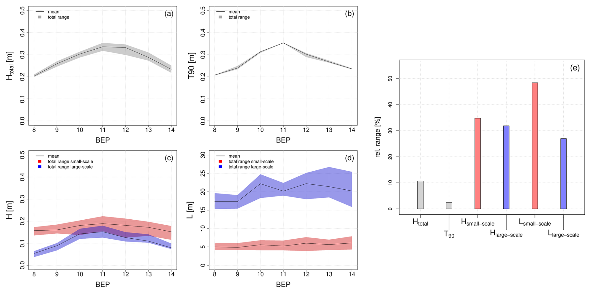
Figure 8 Resulting bedform parameters of the Monte Carlo simulation. (a–d) Identified ranges and mean values for individual BEPs. (e) Averaged relative ranges over BEPs 8–14.

Regarding total bedform height, the T₉₀ parameter remains nearly constant over all iterations for all BEPs, whereas the H_total parameter has a higher scattering with a maximum range of about 5 cm (Fig. 8a and b). The mean for both parameters reaches a maximum in BEP 11 (values of 33 and 35 cm). Considering the individual bedform layers (Fig. 8c and d), the large-scale bedforms appear to be slightly lower (mean values range from 15 to 19 cm for the small-scale bedforms and from 5 cm to 15 cm for the large-scale bedforms) but much longer than the identified small-scale bedforms (mean values range from 5 to 6 m for the small-scale bedforms and from 17 to 22 m for the large-scale bedforms). Bedform lengths appear to be very sensitive with respect to varying input parameter settings. The lengths of the small-scale bedforms have a maximum total range of 4 m, while the lengths of the large-scale bedforms have a maximum total range of up to 10 m in BEP 14. It should be noted that spatial averaging (over the cross section) can lead to a stabilization and thus to a decreased scattering of the results, which is shown in Fig. 8e. The relative ranges ($(\text{max}-\text{min})/\text{mean}$) of the individual parameters are shown here, which were averaged over the BEPs 8–14. By far the lowest values are found for the total bedform height (values of 2 % for T₉₀ and 10 % for H_total). Bedform heights of individual layers show much higher values between 30 % and 35 %. The highest values, however, are found for bedform lengths with a value of almost 50 % for the small-scale bedforms.

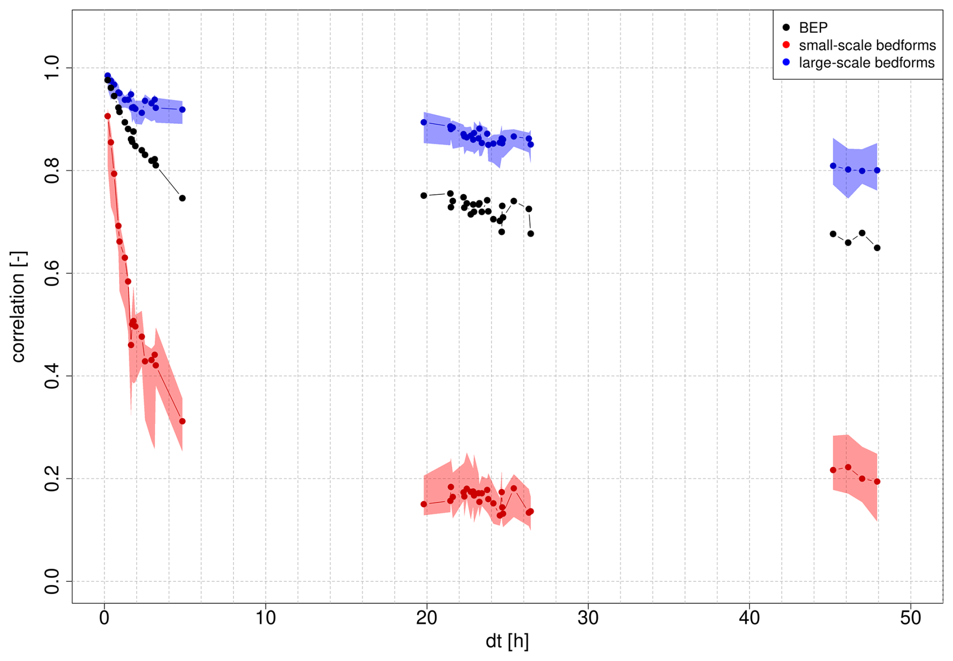
Figure 9 Correlation coefficients from the cross-correlation analysis (method 1) as a function of time difference between successive measurements. The red and blue dots represent the median values for small-scale and large-scale bedforms obtained from MCS, respectively. Polygons show the total range of results. Only one result per measurement is available for the total BEP.

4.3 Bedform migration and bedload transport

To enable the calculation of bedform migration rates, repeated MBES measurements were performed during the campaign with a minimum time difference of 3.2 h between two successive measurements for the entire bedform field. These intervals turned out to be too long to track the faster-migrating small-scale bedforms. Therefore, only the detailed measurements of the single measurement swath in the center (nos. 5–14 in Table A2) are considered for the analysis of migration rates. Here, intervals are much shorter and start from 0.2 h. Based on the 10 available measurements, 45 pairwise combinations can be analyzed (see Table A3). Migration rates were calculated using two different methods, as introduced in Sect. 2.5.

Figure 9 shows the correlation coefficients derived from the cross-correlation analysis (method 1) as a function of time difference dt between two measurements. Correlation coefficients are shown here for the total BEP (without considering separate layers of bedforms) and for the individual layers. The constructed baselines from the MCS were used for considering the individual layers. Accordingly, results from 100 iterations are available for each measurement. For the total BEP, on the other hand, only one result per measurement is available. Correlation coefficients obviously decrease with increasing dt due to the deformation of bedforms. However, correlation coefficients of the large-scale bedforms and of the total BEP remain above a value of 0.7 even after 20 h. Concerning the small-scale bedforms, correlation coefficients decrease much more rapidly and drop below a value of 0.5 after less than 2 h, highlighting that longer time differences between measurements are unsuitable for tracking these bedforms.

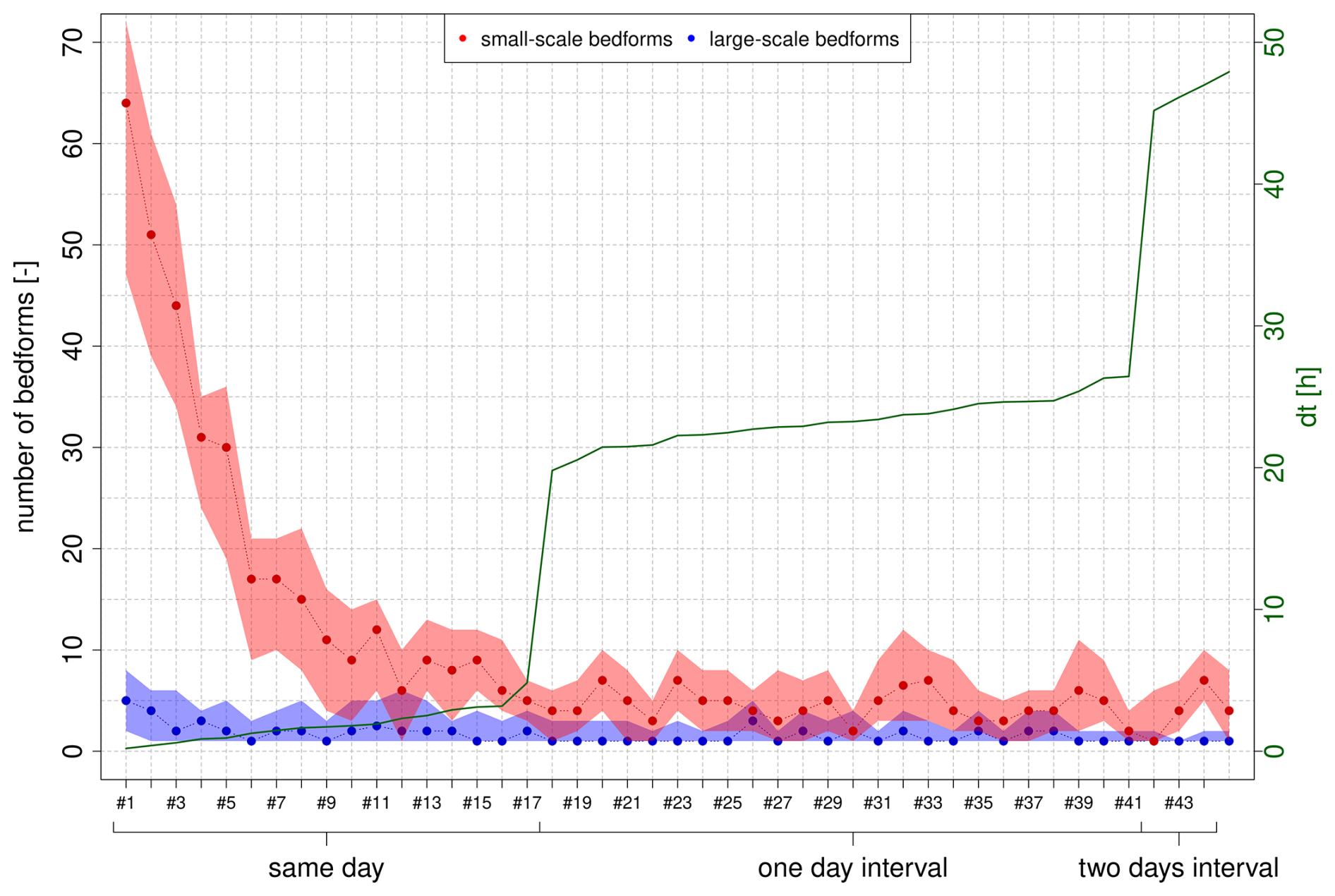
Figure 10 Number of traceable bedforms depending on measurement interval (centroid analysis, method 2). The red and blue dots represent the median values for small-scale and large-scale bedforms obtained from MCS. Polygons show the total range of results.

By using method 2 (centroid analysis), migration rates for individual bedforms are determined. Individual migration rates are then filtered by the defined quality criteria considering the geometrical similarity of corresponding bedforms from two measurements. Figure 10 shows the remaining number of traceable bedforms. For the small-scale bedforms, the number of traceable bedforms strongly decreases as dt increases. For this reason, the results for longer measurement intervals should be assessed with particular caution, as they are influenced by only a few observations. In contrast, the number of traceable large-scale bedforms is low for all measurement pairs and does not change significantly as dt increases, which is why we do not recommend using this method to track underlying large-scale bedforms (see Sect. 5).

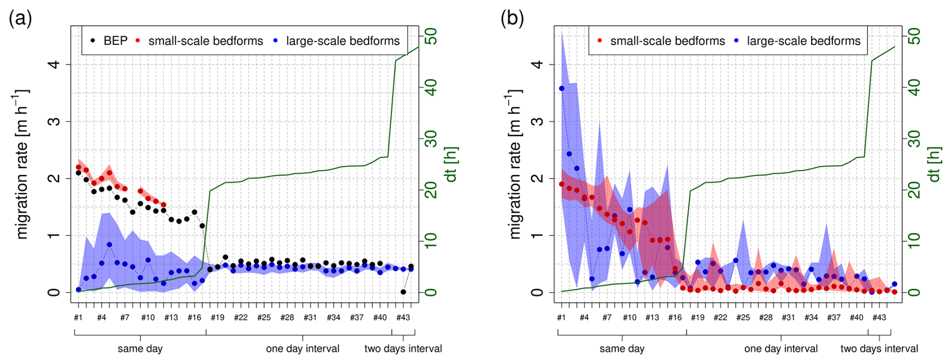
Figure 11 Calculated migration rates for all respected measurement pairs by means of cross-correlation analysis (method 1, a) and centroid analysis (method 2, b).

Figure 11 summarizes determined migration rates for all 45 possible combinations of measurements for both methods. For method 1 (cross-correlation analysis), results with correlation coefficients smaller than 0.5 were excluded. For method 2 (centroid analysis), after filtering the results, outliers exceeding a 95th percentile were removed and then weighted average migration rates were calculated along the BEP.

For method 1 median migration rates of the small-scale bedforms fluctuate between 1.5 and 2.2 m h⁻¹. For all measurement pairs with a time difference of 2.5 h or more (above pair no. 12), the correlation coefficients drop below the 0.5 threshold value, and thus no reliable results are available. For the large-scale bedforms, median migration rates fluctuate between 0.1 and 0.8 m h⁻¹. Fluctuations are much lower for measurement pairs with a time interval of 1 d or more. Concerning migration rates of the total BEPs (without considering individual layers of bedforms), results for short measurement intervals are close to the migration rates of the small-scale bedforms, while results for longer measurement intervals are close to the migration rates of the large-scale bedforms, depending on which process is dominant. This highlights the need for considering individual bedform layers in order to make precise statements about migration rates. Migration rates for both the small-scale bedforms and the BEPs decrease with increasing measurement intervals. This effect can probably be attributed to the fact that small bedforms tend to migrate faster but at the same time can only be reliably tracked for very short measurement intervals. For small dt, the migration of small bedforms has a significant effect on the cross-correlation analysis (and thus on the determination of the best-fitting spatial offset). With increasing dt, deformation of bedforms increases so that the smallest bedforms are no longer traceable and the average migration rate decreases (see also Sect. 5.1.2). This effect can be found in the results of both methods.

Regarding method 2 (Fig. 11b), fluctuations are higher compared to method 1. For the small-scale bedforms, median migration rates vary between 1 and 2 m h⁻¹ for most of the measurement pairs that contain measurements of the same day. For longer measurement intervals (1 or 2 d intervals) values vary between 0 and 0.5 m h⁻¹. As shown in Fig. 10, the number of traceable bedforms drastically decreases with increasing dt, which is why only the results for very short measurement intervals are sufficiently reliable. Here, the results are quite comparable to those of method 1. Again, migration rates decrease with increasing dt. The number of traceable large-scale bedforms is constantly low (≤5). Fluctuations are very high for short measurement intervals. For longer measurement intervals, however, median migration rates are again comparable to those obtained from method 1 and vary from 0.1 to 0.6 m h⁻¹.

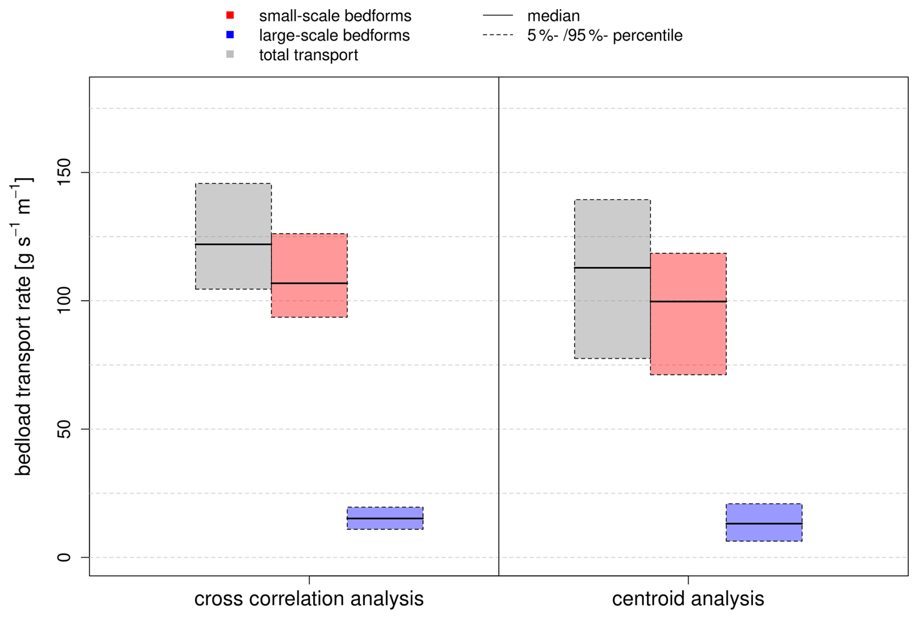
Figure 12 Comparison of bedload transport rates derived from cross-correlation and centroid analysis along the evaluated BEP.

Based on the migration rates calculated by the two methods, bedload transport rates were estimated using Eq. (4). As has been shown, the time difference between two measurements has a strong impact on resulting migration rates. The small-scale bedforms can only be tracked accurately by using short measurement intervals, whereas longer intervals are more suitable for the large-scale bedforms. For this reason, only measurement intervals shorter than 2 h were considered for the estimation of bedload transport due to the small-scale bedforms, whereas only measurement intervals longer than 19 h (measurements carried out on different days) were considered for the large-scale bedforms. For estimating the total transport, the quantities derived from both bedform layers were summed up. Figure 12 shows estimated bedload transport rates and their ranges resulting from the different input parameter settings within the MCS for both methods. The results obtained from the centroid analysis are again more affected, leading to total bedload transport rates fluctuating within a range of about 60 $\mathrm{g}{\mathrm{s}}^{-\mathrm{1}}{\mathrm{m}}^{-\mathrm{1}}$ (corresponding to more than 50 % in relation to the median). In comparison, those obtained from the cross-correlation analysis only fluctuate within a range of about 40 $\mathrm{g}{\mathrm{s}}^{-\mathrm{1}}{\mathrm{m}}^{-\mathrm{1}}$ (corresponding to about 30 % in relation to the median). Median values, however, are of the same order of magnitude for both methods. Further on, both methods indicate that bedload transport associated with the small-scale bedforms accounts for nearly 90 % of the total transport, while bedload transport associated with the large-scale bedforms accounts for only slightly more than 10 %.

5 Discussion

5.1 Interpretation of the results

5.1.1 Bedform geometries

The results for bedform geometries (refer to Sect. 4.2) show the lowest uncertainties for the bedform parameters that measure the total height. Here, we determined values of 2 % for T₉₀ and 10 % for H_total. The heights of the individual layers, on the other hand, show significantly higher uncertainties of 30 % to 35 %. The greatest uncertainties arise in the determination of bedform lengths, which reach values of up to 50 %. We recognized that uncertainties in the determination of bedform geometries are lower if the geometries of the individual layers are considered together as composite entities. In this case, the calculated attributes only depend on the baseline of the large-scale bedforms, which separates the bedforms from the underlying non-active layer of the riverbed. They are independent of the baseline of small-scale bedforms that separates both layers from each other. At the same time, we show in Sect. 5.2 that the window size of the small-scale bedforms is the most sensitive input parameter. This explains why determined uncertainties are lower for total heights compared to the heights of the individual layers.

Furthermore, bedform lengths were subject to higher uncertainties than bedform heights, especially for the small-scale bedforms. The specific morphological situation for the test dataset from the Lower Rhine could have had an influence on this result. It is noticeable that the analyzed bedforms of both layers are rather similar in height and differ mainly in their length (see Fig. 8c and d). For most BEPs both layers have average heights of approx. 10 to 20 cm, while the average lengths are approx. 5 to 6 and 17 to 22 m, respectively. There are other cases where both length and height differ by an order of magnitude, e.g., as in datasets from the Rio Paraná as published in Parsons et al. (2005) or from the Waal river as published in Zomer et al. (2023). The analysis should therefore be continued by using datasets with different morphological conditions in order to validate this finding.

The measurements from the Lower Rhine were carried out a few days after a peak in discharge. Findings from other studies indicate that significant changes in bedform characteristics may occur during the falling flood limb, and these findings are very much in line with our observations for the dataset from the Lower Rhine. According to Martin and Jerolmack (2013), the larger primary bedforms become inactive during the fall of the flood and are cannibalized by the formation of smaller bedforms in equilibrium with the decreased discharge. In the study of Wilbers and Ten Brinke (2003), smaller secondary bedforms were observed emerging during the falling flood limb, while shrinking heights and increasing lengths were observed for primary bedforms. In Zomer et al. (2023), however, secondary bedforms were observed over the full range of flow conditions. To demonstrate that we found similar conditions for the dataset from the Lower Rhine, the height-to-length ratio of detected bedforms is plotted in comparison to the maximum and mean bedform height according to Flemming (1988) in Fig. 13. While the small-scale bedforms fit in quite well with Flemming's ratio, the large-scale bedforms are less steep and are shifted accordingly to the right. Corresponding to the observations of the aforementioned studies, the emergence and migration of small-scale bedforms could have resulted in shrinking heights (and retarded migration) of the large-scale bedforms after the peak in discharge (this would also explain the high contribution of the small-scale bedforms to the total bedload transport). However, no further measurement data are available to confirm this conclusively, as investigating the temporal development of bedforms during a flood wave was not the initial objective of this study.

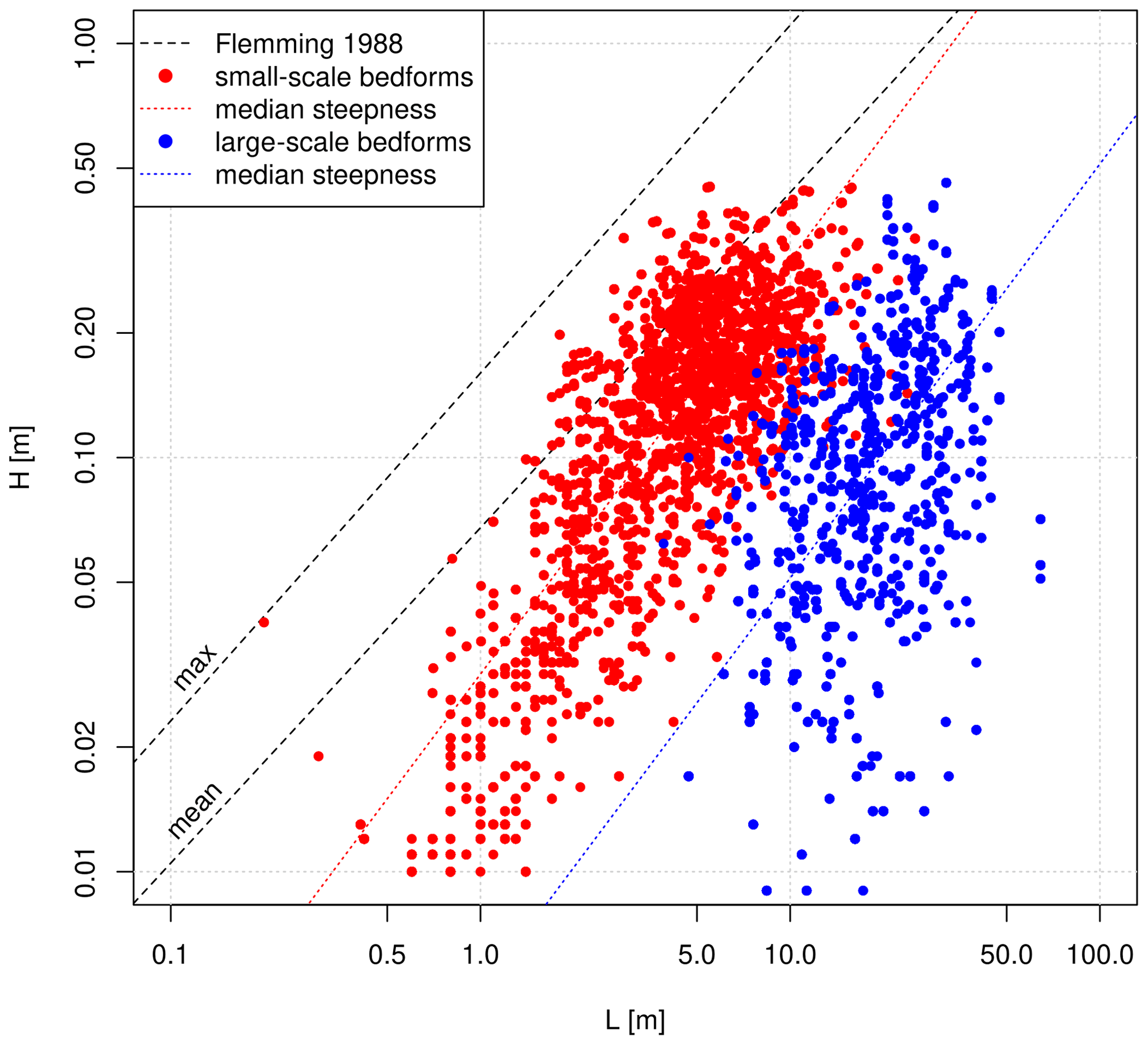
Figure 13 Ratio of identified bedform heights and lengths obtained from MBES data from the Lower Rhine (February 2020) compared to the mean and maximum bedform heights according to Flemming (1988).

The performed MCS revealed high uncertainties in the determination of bedform geometries, which resulted from different input parameter settings. However, there are other sources of uncertainty in the determination of bedform geometry like the choice of method or tool in general. For example, in the recently published meta-analysis by Scheiber et al. (2024), five bedform identification algorithms were compared. They were divided into two groups based on methodological similarities. Within each group deviations in median heights and lengths did not exceed a value of 25 % after efforts were made to standardize inputs (e.g., harmonizing definitions of bedform attributes). Much higher deviations were found between the two groups. Another source of uncertainty is described by Scheiber and Lefebvre (2023). They show that the definition of bedform height (there are various possible and common ways to geometrically determine the height of an individual bedform) can have an even higher influence on the resulting values. Here, relative differences of over 100 % were identified. Further on, the influence of data preprocessing like the generation of DEMs and BEPs could also be considered. By collating all this information about the multiple sources of uncertainty, the picture can be gradually completed.

5.1.2 Bedform migration and bedload transport

In Sect. 4.3 we showed the results for bedform migration that were derived from the MCS by using the multiple solutions obtained from the zero-crossing procedure. We investigated how the influence of the different input parameter settings for the zero-crossing procedure propagates to the determination of bedform dynamics. In addition, the influence of the measurement interval was evaluated. These results reveal that the determined migration rates and their uncertainties depend on the time difference between two measurements. This time difference determines the highest possible traceable migration rate and thus at the same time the minimum bedform dimensions that can be considered (since it is assumed that migration rates increase with decreasing bedform dimensions). Even within an individual layer, there is heterogeneity in terms of bedform dimensions. The smaller the time difference is, the smaller the bedforms that can be tracked accurately will be. An increase in time difference leads to an increasing loss of information and eventually to a potential underestimation of bedform migration and bedload transport rates since the faster-migrating smaller bedforms are no longer identified. In the centroid analysis these are successively removed from the analysis as they no longer meet the defined quality criteria. In the cross-correlation analysis the influence of larger bedforms within an individual layer increases with increasing time difference. This explains the decreasing trend in Fig. 11 regarding the migration rate of the small-scale bedforms, which was found by using both methods. Exceeding a measurement interval of 2 h, migration of small-scale bedforms can no longer be tracked, which eventually leads to an underestimation of bedform migration and bedload transport (it was shown that the migration of small-scale bedforms accounted for about 90 % of the total bedload transport). On the other hand, in order to track the underlying large-scale bedforms, longer measurement intervals appeared to be more suitable as they are subject to significantly lower scattering. For short intervals (measurements carried out on the same day) deviations of more than 100 % were reached in cross-correlation analysis (Fig. 11a). This underlines that in order to track both small- and large-scale bedforms accurately, different intervals and therefore multiple measurements are required. It could be helpful to perform preliminary measurements to get a first impression about prevailing bedform dimensions and migration rates and to select suitable intervals based on this.

In this study, a second method was used for determining bedform dynamics. The newly introduced centroid analysis appeared to be subject to greater uncertainties, especially regarding migration of large-scale bedforms. As shown in Fig. 10 the number of traceable bedforms is constantly low for the large-scale bedforms. We therefore recommend not to use this new method to track underlying large-scale bedforms, since for short measurement intervals the spatial offset is too small to enable a precise assignment (approaching the limit in terms of measurement accuracy), whereas for large intervals deformation already has too much influence on the calculation of the geometric centroids. However, another reason for the smaller number of traceable large-scale bedforms can be found in the distribution of larger bedforms along the BEPs. While small-scale bedforms can be found along the entire BEP, large-scale bedforms are only present in certain sections and are not covering the total length of the BEP. The added value of the new method is a deeper look at the behavior of individual bedforms – in relation to their geometric attributes – as well as information about the longitudinal variability of bedload transport. From this information, new insights can be gained, especially concerning the behavior of rapidly migrating smaller bedforms, which can end up contributing the largest part to the total bedload transport.

As mentioned above, there are multiple sources of uncertainty in the determination of bedform geometries. When deriving bedload transport rates from these, others are added, such as the uncertainty in the estimation of porosity and grain density. For example, since both parameters are linearly related to bedload transport, a variation of 10 % will also result in a change of 10 % concerning bedload transport rates. The choice of an empirical formula for the calculation could even be a further source of uncertainty. Again, these sources of uncertainty must be added in order to complete this consideration.

A more detailed look at the performance of different bedload transport measurement techniques and – among other aspects – at possible factors influencing the dune tracking method were the subject of the so-called LILAR campaign (Onjira et al., 2023). The campaign was carried out in November 2021 through cooperation between German and Dutch authorities. One of the objectives was to compile, compare and evaluate different methods for measuring sediment transport. In addition, we are planning to perform further campaigns to investigate the influence of different discharge conditions on bedform characteristics in more detail. For this kind of comparative study, it is again essential to estimate the uncertainties in bedform analyses in order to robustly evaluate occurring changes.

5.2 Sensitivity of the input parameters

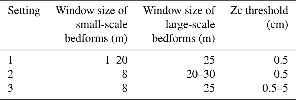
In Sect. 5.1 we discussed the influence of input parameter settings on the calculated bedform characteristics and bedload transport rates. In this section, we discuss which of the input parameters has the greatest influence. A sensitivity analysis was performed in which only one input parameter was varied at a time while the others were kept constant. Table 2 shows the three chosen input parameter settings. For the parameters that were kept constant, a mean value was set based on the results from the wavelet analysis (see Fig. 7).

Table 2 Input parameter for sensitivity analyses.

5.2.1 Bedform geometries

Figure 14 shows the potential influence of the input parameters window size for small- (a–c) and large-scale bedforms (d–f) and zc threshold (g–i) on the resulting bedform geometries (T₉₀, H_total L_{1, 2/total}). The resulting bedform geometries were averaged over the considered BEPs 8–14. Increasing the window size for the small-scale bedforms (setting 1) results in increasing bedform heights and lengths. The parameter is especially sensitive during the first iterations. When exceeding a value of about 5 m, increasing convergence can be observed for both bedform heights and lengths. Within the selected range of window sizes based on the wavelet analysis (gray area), only a very low variability can be observed. Thus, the sensitivity is particularly high outside this selected range. Overall, with respect to bedform height, the T₉₀ parameter behaves less sensitively than the H_total parameter. The reason for this is that the T₉₀ parameter is independent of the number of identified bedforms. It is not based on measuring individual bedform heights but on measuring the accumulated bedform layer thickness (T) in every x position along the entire BEP. Therefore, the same number of input values is always used for the calculation.

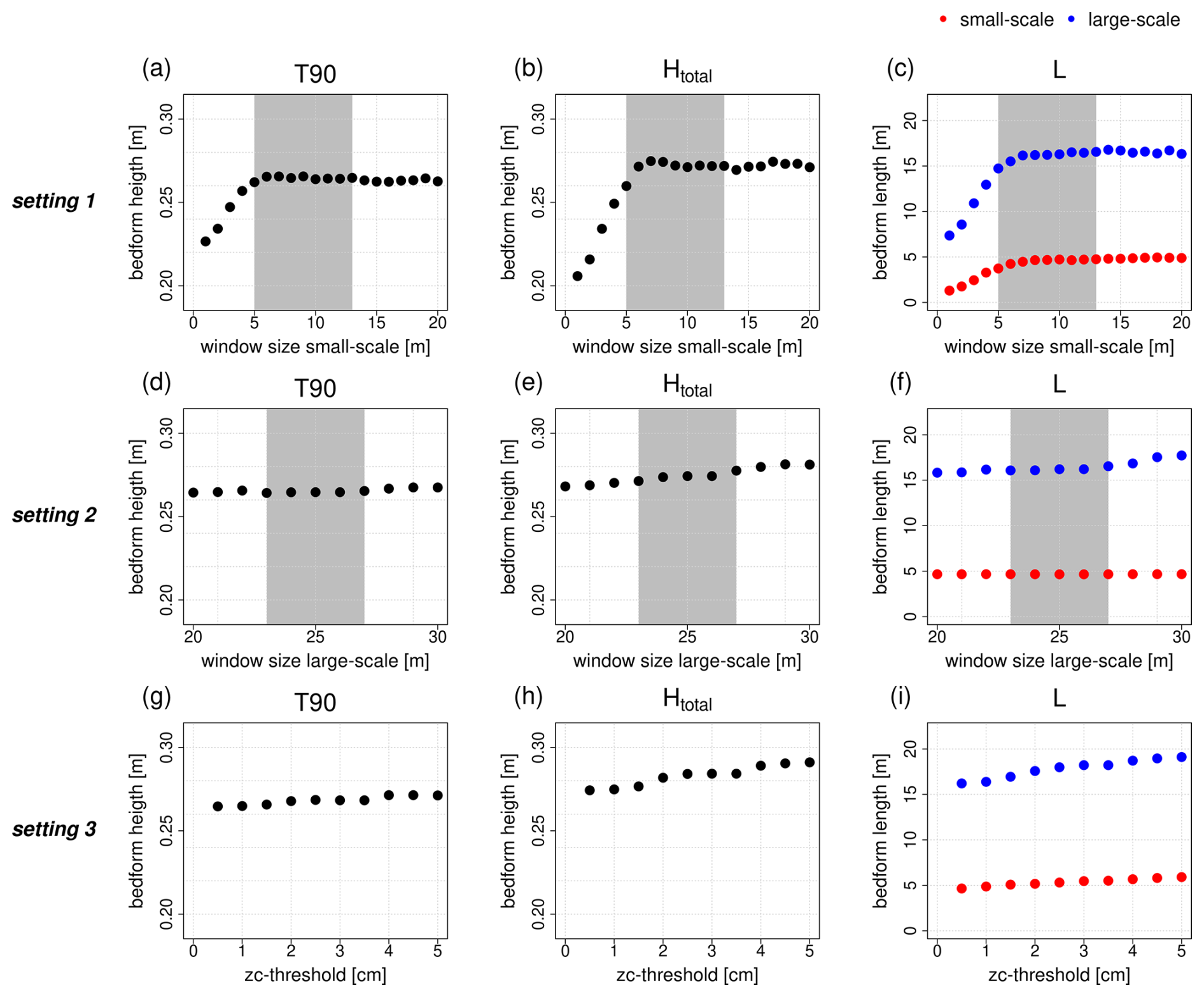
Figure 14 Influence of variation in the input parameters on derived bedform geometries (the gray area corresponds to the selected value range based on the wavelet analysis). Setting 1 uses a small-scale window size of 1–20 m, a large-scale window size of 25 m and a zc threshold of 0.5 cm. Setting 2 uses a small-scale window size of 8 m, a large-scale window size of 20–30 m and a zc threshold of 0.5 cm. Setting 3 uses a small-scale window size of 8 m, a large-scale window size of 25 m and a zc threshold of 0.5–5 cm.

The window size for the large-scale bedforms (setting 2) has almost no influence on the T₉₀ parameter (Fig. 14d). With respect to the H_total parameter, a very slight increase (2 cm) can be observed with increasing window size (Fig. 14e). Bedform length (in this case only the large-scale bedforms are affected) again exhibits more sensitivity. Here, no convergence can be observed (Fig. 14f). Nevertheless, variability is much smaller compared to setting 1. It can be assumed that convergence will eventually occur with increasing values as the calculated moving average value successively approaches a horizontal line.

The influence of the zc threshold (setting 3) is also much smaller than that of the window size for the small-scale bedforms. Bedform heights exhibit less sensitivity than bedform lengths, for which no convergence occurs (Fig. 14i). By increasing the zc threshold, local minima are filtered out successively (see Sect. 2.3). Thereby, several individual bedforms are summarized, resulting in a smaller number of longer bedforms. While the maximum height is limited by the lowest and the highest point in a BEP, a successive increase in length – by combining several individual bedforms – is technically possible. This is why it is important to consider the expected bedform dimensions in advance in order not to obtain implausible results.

Changing the window size for the small-scale has the strongest impact on resulting bedform geometries. Concerning bedform height, the T₉₀ parameter appears to be more robust towards varying input parameter settings compared to the H_total parameter. Overall, bedform lengths appear to be more sensitive and include a higher degree of uncertainty. While the H_total parameter shows a maximum variability of about 30 %, the total length (corresponding to the length of the large-scale bedforms) shows a maximum variability about 60 % (both for setting 1). The delineation of two adjacent bedforms is not always obvious, and several different solutions might be conceivable. Even a manual delineation is a highly subjective process and could lead to different solutions for different investigators. In many cases a convergence pattern can be observed that starts at the lower margin of window sizes based on the results from the wavelet analysis (shaded gray area in Fig. 14). Window sizes smaller than the lower margin lead to diverging results, which confirms the need for performing the wavelet analysis as an orientation.

These findings should be taken into account when analyzing bedform geometries, such as studies on the relationship between bedform height and length (e.g., Flemming 1988; Lefebvre et al., 2022). Individual bedform attributes are often displayed in scatterplots. According to the findings of this study, an uncertainty range would have to be specified for each data point in a scatterplot based on different input parameter settings in the evaluation procedure. Therefore, we would recommend investigating the sensitivity of input parameters for other methods as well. The shown results provide an indication of the possible order of magnitude.

5.2.2 Bedform migration and bedload transport

Figure 15 shows the results of the sensitivity analysis for the calculation of bedform migration and bedload transport rates based on the cross-correlation analysis (method 1). For this purpose, the resulting parameters were averaged over different measurement intervals. Based on the findings presented in Sect. 4.3, only measurement intervals shorter than 2 h were considered for the small-scale bedforms, whereas only measurement intervals longer 19 h (measurements carried out on different days) were considered for the large-scale bedforms.

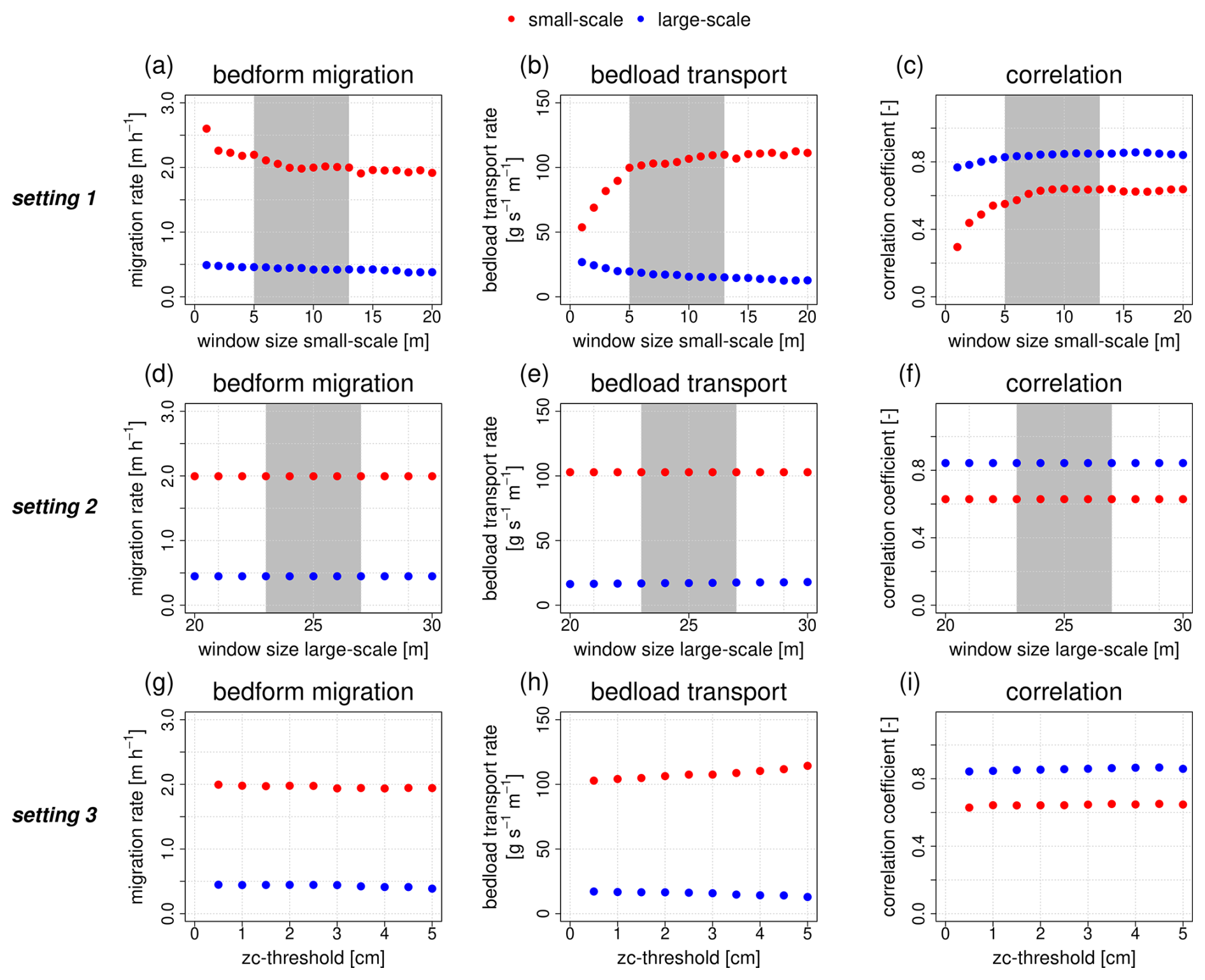
Figure 15 Influence of variation in the input parameters on the cross-correlation analysis (the gray area corresponds to the selected value range based on the wavelet analysis). Setting 1 uses a small-scale window size of 1–20 m, a large-scale window size of 25 m and a zc threshold of 0.5 cm. Setting 2 uses a small-scale window size of 8 m, a large-scale window size of 20–30 m and a zc threshold of 0.5 cm. Setting 3 uses a small-scale window size of 8 m, a large-scale window size of 25 m and a zc threshold of 0.5–5 cm.

Increasing window sizes for the small-scale bedforms lead to decreasing bedform migration rates that converge to a value of about 2 m s⁻¹ for window sizes >5 m (Fig. 15a). For smaller window sizes, smaller bedforms are derived from the BEPs, which are migrating at higher rates. At the same time, bedload transport rates for the small-scale bedforms increase with increasing window size as bedform area increases, which outweighs the influence of decreasing migration rates. They converge to a value of about 110 $\mathrm{g}{\mathrm{s}}^{-\mathrm{1}}{\mathrm{m}}^{-\mathrm{1}}$ (Fig. 15b). Bedform area for the large-scale bedforms, however, decreases with increasing bedform area for the small-scale bedforms due to a different delineation of the total geometry. As a result, bedload transport rates for the large-scale bedforms decrease as well. Correlation coefficients increase with increasing window size for the small-scale bedforms (Fig. 15c). This is because small bedforms resulting from small window sizes can only be traced accurately for very short measurement intervals. Thus, averaged correlation coefficients are lower for smaller window sizes. The large-scale bedforms are only slightly affected. Overall, highest variability can be found outside the chosen range of window sizes for the small-scale bedforms based on the wavelet analysis.

Varying window sizes for the large-scale bedforms do not have any influence on the cross-correlation analysis. This is because the baselines of the large-scale bedforms are not included in the analysis (see Sect. 2.5). Only the changing (increasing) bedform areas result in a slight increase in bedload transport rates for the large-scale bedforms (Fig. 15e).

Concerning the behavior of the zc threshold, similar effects can be observed as for the window size for the small-scale bedforms at setting 1; however, they turn out to be significantly less sensitive (Fig. 15g–i). Correlation coefficients stay rather constant over all iterations (Fig. 15i).

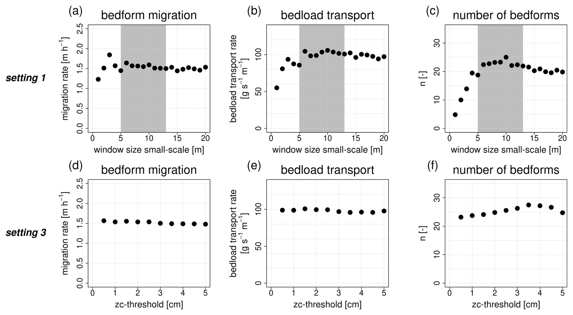
Figure 16 Influence of variation in the input parameters on the centroid analysis (the gray area corresponds to the selected value range based on the wavelet analysis). Setting 1 uses a small-scale window size of 1–20 m, a large-scale window size of 25 m and a zc threshold of 0.5 cm. Setting 2 uses a small-scale window size of 8 m, a large-scale window size of 20–30 m and a zc threshold of 0.5 cm. Setting 3 uses a small-scale window size of 8 m, a large-scale window size of 25 m and a zc threshold of 0.5–5 cm.

Figure 16 shows the influence of input parameter settings on the centroid analysis (method 2). As explained in the previous sections, the method is rather suitable for small-scale bedforms and short measurement intervals. This is why the small-scale bedforms and only those measurement pairs with intervals shorter than 2 h are considered here (see Sect. 4.3).

At setting 1, migration rates initially increase with increasing window size (Fig. 16a). A maximum is reached at a value of 3 m. A further increase in window size leads to decreasing migration rates with a tendency of convergence to a value of 1.5 m s⁻¹. Bedload transport rates first increase and then tend towards a value of 100 $\mathrm{g}{\mathrm{s}}^{-\mathrm{1}}{\mathrm{m}}^{-\mathrm{1}}$ (Fig. 16b). Very small bedforms can only be traced accurately at very short measurement intervals, meaning that a rapid increase in the number of detected bedforms can be observed with increasing window size (Fig. 16c). After reaching a maximum at a value of 10 m, the number of traceable bedforms decreases again. An increasing window size leads to increasing bedform areas and thus to a decreasing number of bedforms. For all parameters the highest variations are again found outside the chosen range of window sizes.

Varying the setting of the zc threshold again has much less impact on the results. No systematic effect on the centroid analysis can be observed (Fig. 16d and e).

As for bedform geometries, it can also be observed for bedform migration and bedload transport that setting 1 has the greatest influence on the resulting parameters. This is true for both methods. Outside the chosen range of window sizes based on the results from the wavelet analysis, increasing divergence can again be seen. The results illustrate that the effect of varying input parameter settings in the zero-crossing procedure propagates to the determination of bedform dynamics.

6 Conclusions

Bedform analysis tools are sensitive to the influence of input parameters. Often, no theoretically sound criteria are available for the setting of input parameters with specific values. Thus, this decision depends on the subjective assessment of the investigator. Therefore, we developed a highly automated workflow, which allows for the quantification of uncertainties in the calculation of bedform parameters due to different input parameter settings by an MCS routine. We implemented different methods to analyze both bedform geometry and dynamics (migration and bedload transport). In terms of bedform geometry, we combined a wavelet analysis based on Bedforms-ATM (Gutierrez et al., 2018) with the well-established and widely used zero-crossing procedure. In terms of bedform dynamics, we implemented a cross-correlation analysis and the newly introduced centroid analysis. By applying this workflow to a test dataset from the Lower Rhine in Germany, the following main results and key conclusions can be derived.

Bedform parameters react with different sensitivity to varying input parameter settings. The lowest uncertainties were found when individual layers of bedforms were considered together as composite entities without discriminating between them. The introduced T₉₀ parameter proved to be especially robust as a measure of total bedform height with uncertainties of only 2 %. Uncertainties in the heights of individual bedform layers, on the other hand, appeared to be much higher (between 30 % and 35 %). The highest uncertainties were identified for bedform lengths, reaching values of up to 50 % for the small-scale bedforms. Uncertainties regarding bedform geometries are propagated to the determination of bedform migration and bedload transport rates.

Dune-tracking-induced uncertainties for bedload transport rates were found to be on the order of 30 % (by using the cross-correlation analysis) to 50 % (by using the centroid analysis). By applying both methods it could be shown that the migration of the small-scale bedforms accounted for about 90 % of the total bedload transport.

Regarding bedform dynamics, there is also an uncertainty due to varying time differences between two consecutive measurements. Rapidly migrating secondary bedforms were only traceable for measurements with time differences of less than 2 h. For those measurements a decrease in migration rate was observed for increasing time differences. On the other hand, using longer measurement intervals for tracking the underlying large-scale bedforms resulted in lower uncertainties. We therefore recommend choosing measurement intervals with care depending on the process under investigation. Performing preliminary measurements to get a first impression about prevailing conditions may support this decision.

With regard to the question of which input parameter has the greatest influence on the resulting bedform parameters, the window size for the small-scale bedforms exhibited the highest sensitivity. An increase in window size has a significant impact on bedform geometries, bedform migration and bedload transport rates, especially for very small values.

The most stable results were found inside the range of values provided by the wavelet analysis (based on Bedforms-ATM) in the first step of the workflow. This underlines the importance of performing the wavelet analysis to narrow the range of values entering the MCS. It was shown that values below the specified range strongly influence the results and lead to divergence.

Overall, it was shown that varying input parameter settings can have a large influence on the determination of bedform parameters. At the same time, we have introduced a workflow that can provide proof of robust estimates of these parameters. We therefore recommend carrying out similar investigations for other bedform analysis methods and datasets in order to assess the robustness of derived results. However, in this study we focused on the uncertainties resulting from varying input parameter settings. There are multiple sources of uncertainties in bedform analyses like the choice of a method or tool in general or the geometric definitions of bedform attributes. All of these uncertainties must be considered together in field studies characterizing prevailing bedform conditions derived from measurement data.

Appendix A

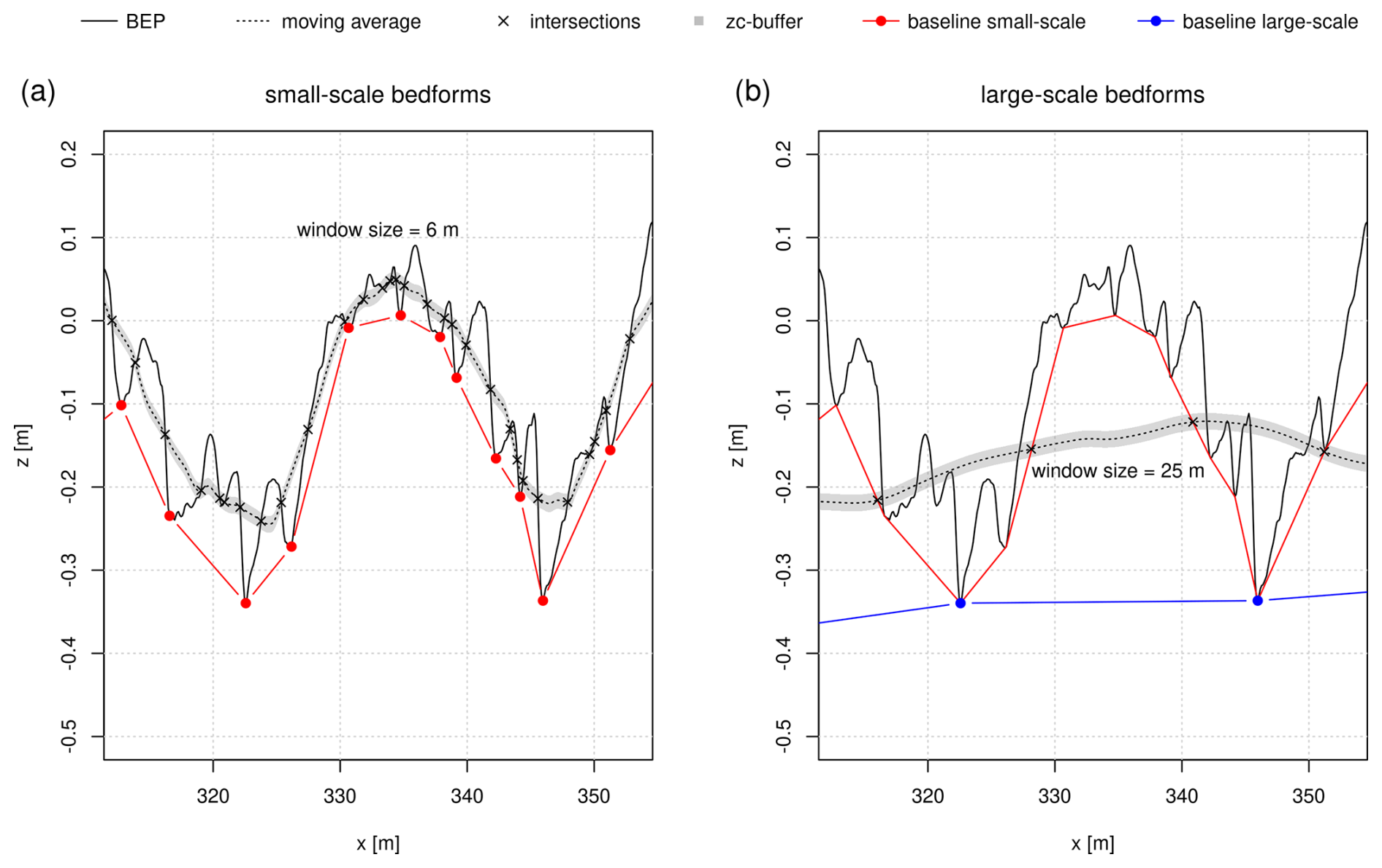
Figure A1 Zero-crossing procedure. (a) Calculation of the baseline of the small-scale bedforms. (b) Calculation of the baseline of the large-scale bedforms.

Figure A2 All BEPs derived from MBES data of the first measurement from 17 February 2020.

Table A1 Definition of bedform parameters.

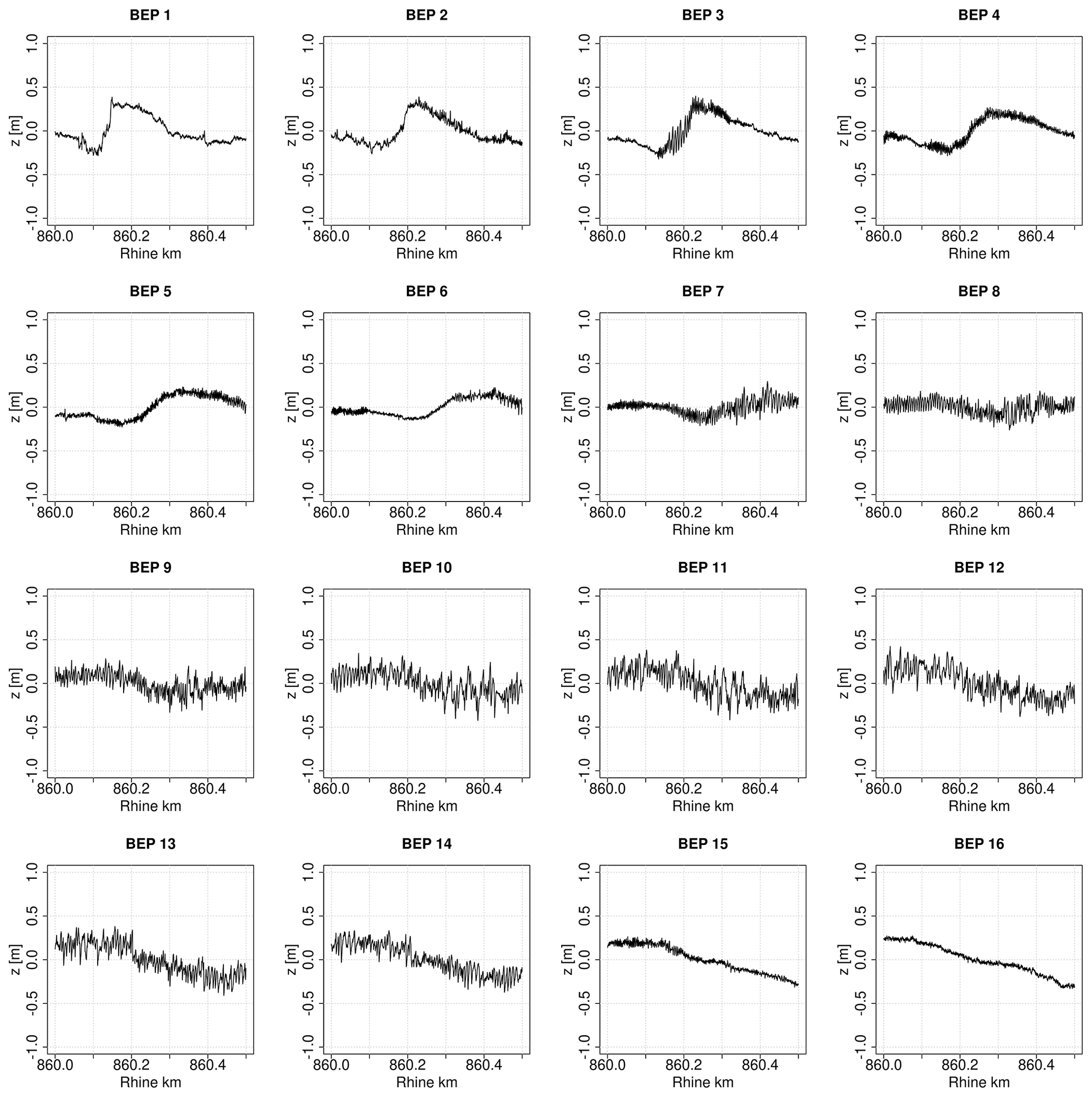
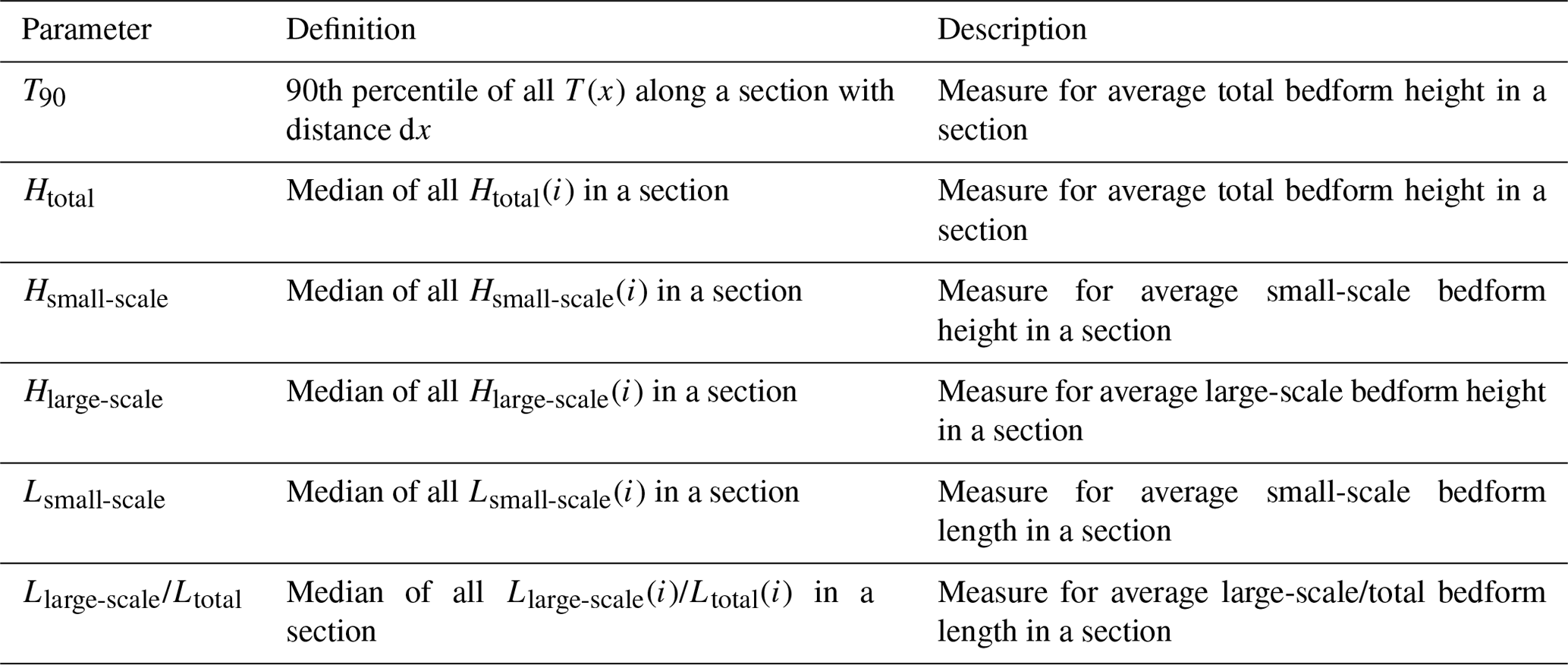
Table A2 Performed MBES measurements during the field campaign.

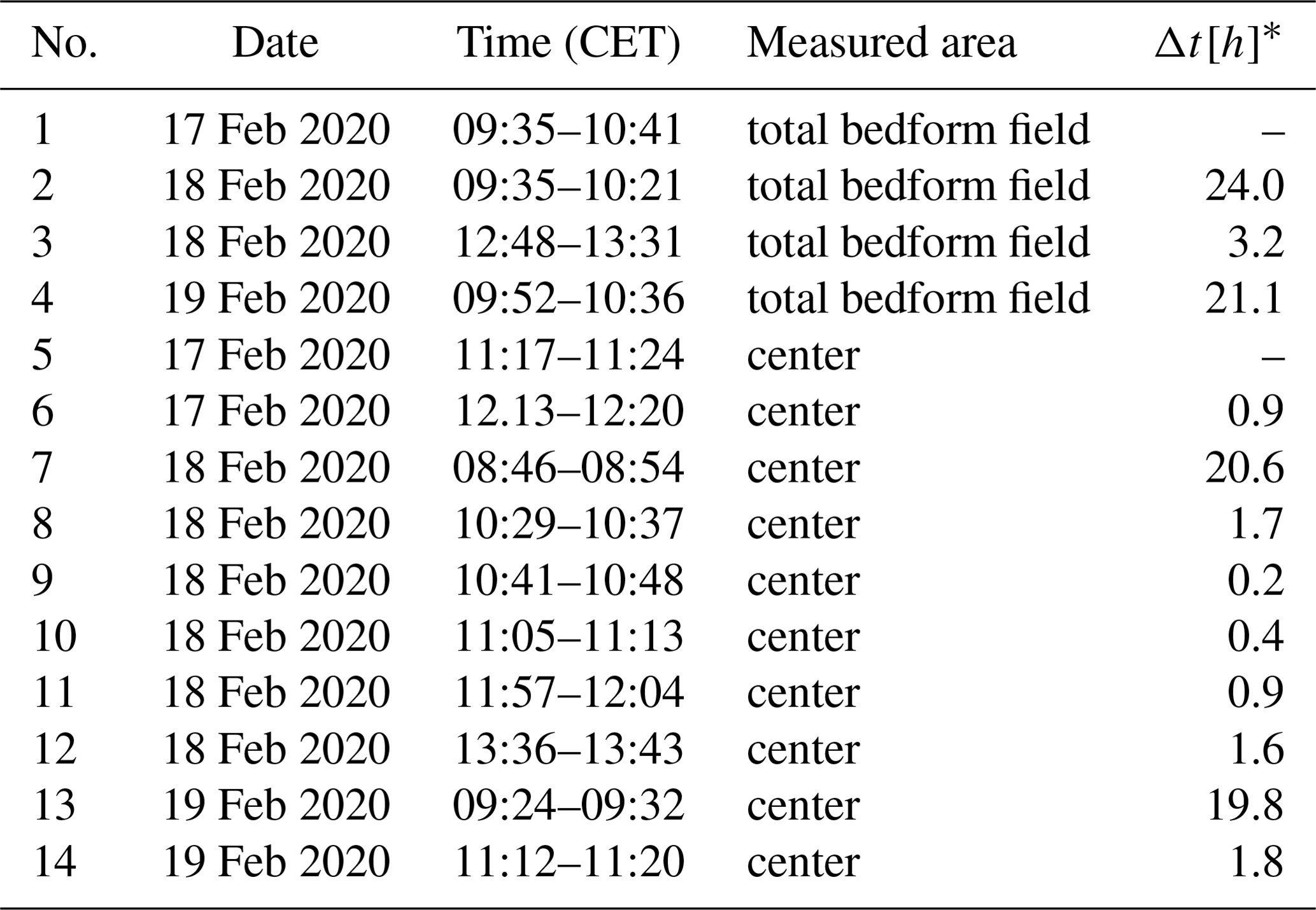
^* time difference to previous measurement.

Table A3 The 45 evaluated measurement pairs obtained from the detail measurements.