Short communication: Multiscale topographic complexity analysis with pyTopoComplexity

pyTopoComplexity is a Python package designed for efficient and customizable quantification of topographic complexity using four advanced methods: two-dimensional continuous wavelet transform analysis, fractal dimension estimation, rugosity index, and terrain position index calculations. This package addresses the lack of open-source software for these advanced terrain analysis techniques essential for modern geomorphology and geohazard research, enhancing data comparison and reproducibility. By assessing topographic complexity across multiple spatial scales, pyTopoComplexity allows users to identify characteristic morphological scales of studied landforms. The software repository also includes a Jupyter Notebook that integrates components from the surface-process modeling platform Landlab (Hobley et al., 2017), facilitating the exploration of how terrestrial processes, such as hillslope diffusion and stream power incision, drive the evolution of topographic complexity over time. When these complexity metrics are calibrated with absolute age dating, they offer a means to estimate in situ hillslope diffusivity and fluvial erodibility, which are critical factors in determining the efficiency of landscape recovery after significant geomorphic disturbances such as landslides. By integrating these features, pyTopoComplexity expands the analytical toolkit for measuring and simulating the time-dependent persistence of geomorphic signatures against environmental and geological forces.

1 Introduction and overview of the package

Topographic complexity, often referred to as topographic roughness or surface roughness, provides critical insights into surface processes and the interactions among the geosphere, biosphere, and hydrosphere (Dietrich and Perron, 2006; Wilson et al., 2007). With the increasing availability of digital terrain model (DTM) data, quantifying topographic complexity has become an essential step in terrain analysis across various research fields. This necessity spans applications such as terrain classification and mapping at various spatial scales (e.g., Weiss, 2001; Robbins, 2018; Lindsay et al., 2019; Pardo-Igúzquiza and Dowd, 2022b, a), evaluating the depositional age of hazardous event sedimentation (e.g., landslides, terrace creation due to avulsions on alluvial fans) and subsequent erosion processes (e.g., Hetz et al., 2016; Johnstone et al., 2018; Booth et al., 2017; Herzig et al., 2024; LaHusen et al., 2020; Woodard et al., 2024; Doane et al., 2024), estimating soil organic carbon storage and nutrient dynamics in landscapes (e.g., Hunter et al., 2024), and identifying habitats to assess ecological diversity on land and on the seafloor (e.g., Frost et al., 2005; Hetz et al., 2016; Wilson et al., 2007).

In recent years, several advanced methods for quantifying topographic complexity have been developed, including two-dimensional continuous wavelet transform (2D-CWT) analysis (Booth et al., 2009; Berti et al., 2013), fractal dimension (FD) estimation (Taud and Parrot, 2005; Glenn et al., 2006; Robbins, 2018; Pardo-Igúzquiza and Dowd, 2020), and rugosity index (RI) calculation (Jenness, 2004; Du Preez, 2015). These newer metrics were developed to better identify complexity signals from surface morphology at various spatial scales of interest and are considered effective in capturing geomorphic features associated with physical and ecological processes relative to traditional metrics like slope, relief, or curvature (e.g., Wilson et al., 2007; Badgley et al., 2017; Booth et al., 2017). Despite their importance, comprehensive publicly available tools that incorporate these advanced methods are lacking. Common open-source geospatial analysis software, such as QGIS (QGIS Development Team, 2024), GRASS GIS (GRASS Development Team, 2024), and WhiteboxTools (Lindsay, 2016), only implement basic conventional methods, limiting the reproducibility and comparability of these newer approaches. Although specialized programs for calculating the RI exist (Walbridge et al., 2018; Benham, 2022), they have been confined to marine bathymetric studies and involve various mathematical limitations, assumptions, and designs.

To address this gap, we have developed an open-source Python toolkit called pyTopoComplexity. This toolkit offers computationally efficient and easily customizable implementations for performing and visualizing the results of 2D-CWT, FD, and RI calculations (Fig. 1). Additionally, pyTopoComplexity includes a module for calculating the terrain position index, a widely used metric in geomorphology research (Newman et al., 2018; Deumlich et al., 2010; Liu et al., 2011) and often used alongside RI in marine geological and ecological studies (Wilson et al., 2007; Walbridge et al., 2018). Each module of pyTopoComplexity includes a corresponding example Jupyter Notebook file with usage instructions. These examples utilize 3 ft (∼0.9144 m) resolution lidar bare Earth DTM data (Washington Geological Survey, 2023) from the 2014 Oso deep-seated landslide along the North Fork Stillaguamish River valley in Washington State, USA (Iverson et al., 2015; Wartman et al., 2016; Collins and Reid, 2019). In the software repository, we also include an additional Jupyter Notebook file Landlab_simulation.ipynb, which allows users to simulate the change of topographic complexity over time via terrestrial processes including non-linear hillslope diffusion (Roering et al., 1999) and fluvial stream power incision (Whipple and Tucker, 1999; Braun and Willett, 2013). This is achieved by running the landscape evolution simulation in the Landlab environment (Hobley et al., 2017) and integrating it with the functionality of pyTopoComplexity.

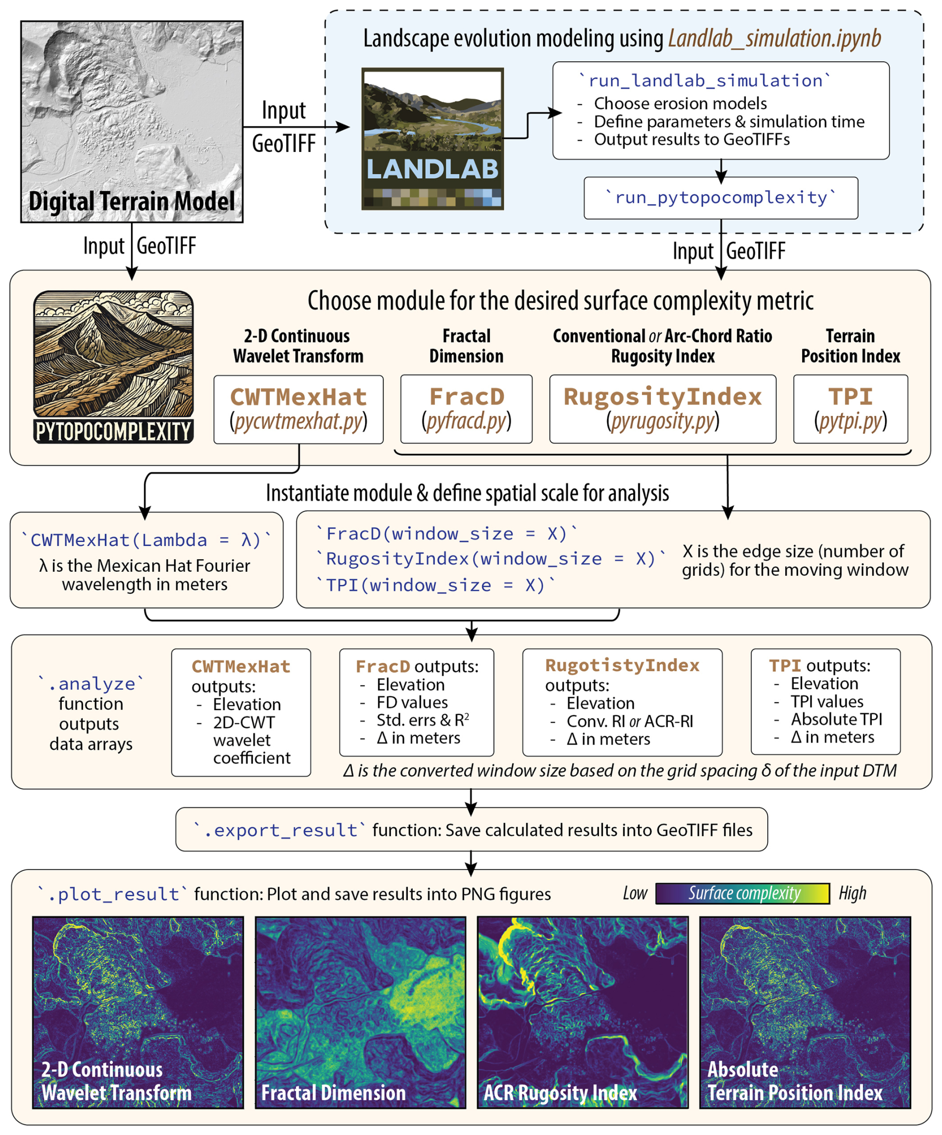
Figure 1 Schematic diagram illustrating the workflow of applying pyTopoComplexity in surface complexity analyses.

2 Methods

The pyTopoComplexity package is available for installation on Windows, Linux, and macOS systems. Users can install it directly from the Python Package Index (PyPI) using the pip command pip install pytopocomplexity or from the conda-forge repository by using the conda package manager with the command conda install pytopocomplexity. Alternatively, users can clone the pyTopoComplexity GitHub repository (https://github.com/GeoLarryLai/pyTopoComplexity, last access: 10 March 2025) to a local directory and then use the conda command conda env create -f environment.yml to create a Python environment with the necessary packages installed.

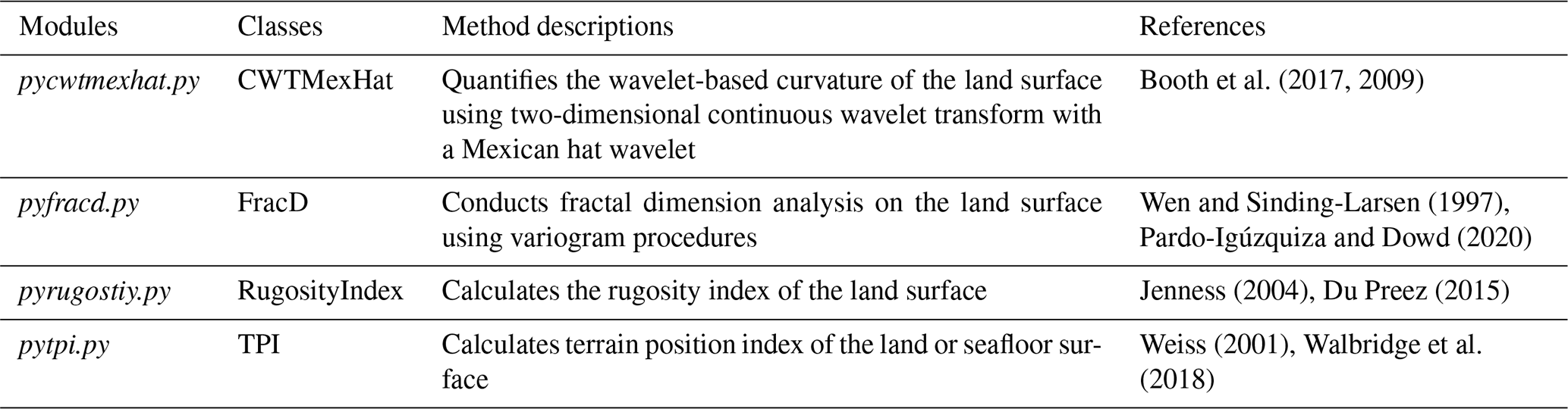
This package includes four modules for performing two-dimensional continuous wavelet transform analysis (2D-CWT), fractal dimension (FD) estimation, rugosity index (RI) calculation, and terrain position index (TPI) calculation (Table 1). Users only need to specify the directories for input and output files, as well as the spatial scale for analysis (e.g., the Fourier wavelength, λ) for the Mexican hat wavelet (i.e., 2D Ricker or Marr wavelet) in 2D-CWT analysis or the size of the moving window (Δ) for other methods. When loading a raster DTM file (acceptable in the GeoTIFF format) into pyTopoComplexity, the toolkit automatically detects grid spacing and units of the projected coordinate system (supported units include meters, US survey feet, and international feet) and applies any necessary unit conversions to maintain consistency in analysis (Fig. 1). By default, results from nodes affected by edge effects due to no-data values are excluded. Users can specify the appropriate spatial scale for their research and select computational methods (e.g., chunk processing, faster mathematical approximations) to optimize performance.

Table 1 Modules contained in the pyTopoComplexity package.

2.1 Two-dimensional continuous wavelet transform (2D-CWT) analysis

The pycwtmexhat.py module in pyTopoComplexity implements the 2D-CWT method for terrain analysis, providing detailed information on how amplitude is distributed across spatial frequencies at each position in the data by transforming spatial data into position–frequency space. When used with the Gaussian family of wavelets, this method is particularly effective for depicting the Laplacian of topography (Torrence and Compo, 1998; Lashermes et al., 2007), revealing concave and convex regions of topography at various smoothing-length scales (Malamud and Turcotte, 2001; Struble et al., 2021; Perron et al., 2008b), identifying deep-seated landslides (Booth et al., 2009; Berti et al., 2013), and estimating the depositional chronologies for landslides (Booth et al., 2017; Herzig et al., 2024; LaHusen et al., 2020; Underwood, 2022) as well as alluvial-fan avulsions (Johnstone et al., 2018).

The 2D-CWT is computed by convolving the elevation data z with a wavelet family ψ at every location (x,y):

$$\begin{array}{}\text{(1)}& C(s,x,y)={\mathit{\delta }}^{\mathrm{2}}{\int }_{-\mathrm{\infty }}^{\mathrm{\infty }}{\int }_{-\mathrm{\infty }}^{\mathrm{\infty }}z(x,y)\mathit{\psi }(x,y)\mathrm{d}x\mathrm{d}y,\end{array}$$

where the resultant wavelet coefficient $C(s,x,y)$ provides a measure of how well the wavelet ψ matches the elevation (z) at each grid point (Torrence and Compo, 1998). δ is the grid spacing of the input DTM raster. The 2D-CWT method isolates specific landform features at the scale of the designated wavelength while filtering out noise from terrain variations at longer or shorter wavelengths. In this implementation, we use the Mexican hat wavelet function to define ψ (Ricker, 1943):

$$\begin{array}{}\text{(2)}& \mathit{\psi }=-{\displaystyle \frac{\mathrm{1}}{\mathit{\pi }(s\mathit{\delta }{)}^{\mathrm{4}}}}\left(\mathrm{1}-{\displaystyle \frac{x^{\mathrm{2}}+y^{\mathrm{2}}}{\mathrm{2}{s}^{\mathrm{2}}}}\right)e^{\left(-\frac{x^{\mathrm{2}}+y^{\mathrm{2}}}{\mathrm{2}{s}^{\mathrm{2}}}\right)},\end{array}$$

which depicts concave and convex landforms according to the wavelet scale s. When s is large, ψ is spread out, capturing long-wavelength features of z; when s is small, ψ becomes more localized, making it sensitive to fine-scale features of z. The Mexican hat wavelet, as defined above, corresponds to the second derivative of a Gaussian envelope. Its Fourier wavelength (λ) depends on the chosen wavelet scale (s) and the grid spacing (δ) of the input DTM raster:

$$\begin{array}{}\text{(3)}& \mathit{\lambda }={\displaystyle \frac{\mathrm{2}\mathit{\pi }s}{\sqrt{\mathrm{5}/\mathrm{2}}}}\mathit{\delta }.\end{array}$$

Users can specify the wavelength λ in meters as the target spatial scale for land surface complexity analysis (Fig. 1). The pycwtmexhat.py module will automatically compute the wavelet scale s based on the grid spacing (δ) of the input raster file. In this module, users can choose to perform convolution either in the original domain (i.e., direct convolution) or in the frequency domain (i.e., using fast Fourier transform) with the “convolve2d” and “fftconvolve” functions from the SciPy package, respectively (Virtanen et al., 2020). By default, the module uses the fftconvolve function for greater computational efficiency.

We note that the equations for C and ψ presented here are mathematical approaches adopted in recent publications (Herzig et al., 2024; LaHusen et al., 2020; Underwood, 2022) on landslide mapping and age dating studies. There are minor differences in the proportionality constant used to define ψ and the conventions used to present the magnitude of the wavelet coefficients C, compared to earlier similar research (Booth et al., 2009). Specifically, Booth et al. (2009) used a different proportionality constant in order to calculate a power spectrum for a range of spatial frequencies rather than curvature, while Booth et al. (2017) reported the mean of C² rather than mean of its absolute value. These differences in mathematical approach will by definition result in different units and order of magnitude (e.g., C² values around 10⁻³ to 10⁻⁴ m⁻² in Booth et al., 2017, and prior studies; C values around 10⁻² to 10⁻³ m⁻¹ in LaHusen et al., 2020, thereafter). Despite this discrepancy, the complexity measures yielded from these approaches that only differ in their proportionality constant are linearly scaled and interconvertible (Fig. S1 in the Supplement), and they both reflect identical spatiotemporal patterns of topographic complexity (i.e., surface roughness).

2.2 Fractal dimension analysis

The pyfracd.py module in pyTopoComplexity calculates the fractal dimension (FD), which measures the fractal characteristics of natural features (Mandelbrot and Wheeler, 1983). This method provides insights into the self-similarity of landscapes, helping quantify their irregularity and fragmentation, which is crucial for studying the essence of the surface topography (Xu et al., 1993; Pardo-Igúzquiza and Dowd, 2020). A surface with a higher FD (closer to 3) indicates a rougher surface with more complex topographic structures, revealing additional irregularities at smaller scales and appearing self-similar across multiple levels of observation. Conversely, a surface with a lower FD (closer to 2) generally reflects a smoother or less detailed plane, where little new complexity emerges at finer scales.

In this module, we adapt the variogram method to estimate the local FD within a moving window centered at each cell of the DTM (Taud and Parrot, 2005; Pardo-Igúzquiza and Dowd, 2022a, b). This approach simplifies the problem to estimating the FD of one-dimensional topographic profiles (Dubuc et al., 1989) within a two-dimensional moving window. For a one-dimensional profile of length R ($r=\mathrm{1},\mathrm{\dots },R$), the variogram γ₁(p) can be estimated at the P lag distances ($p=\mathrm{1},\mathrm{\dots },P$) by

$$\begin{array}{}\text{(4)}& {\mathit{\gamma }}_{\mathrm{1}}\left(p\right)={\displaystyle \frac{\mathrm{1}}{\mathrm{2}(R-p)}}\sum _{r=\mathrm{1}}^{R-p}\left[z\right(i)-z(i+r){]}^{\mathrm{2}},\end{array}$$

where z(i) is the elevation at location i along the profile. The local FD is estimated from one-dimensional profiles in principal directions (i.e., horizontal, vertical, and diagonal) within a square moving window. Assuming that fractional Brownian motion is an appropriate stochastic model for natural surfaces, its variogram follows a power-law model with respect to p (Wen and Sinding-Larsen, 1997),

$$\begin{array}{}\text{(5)}& {\mathit{\gamma }}_{\mathrm{1}}\left(p\right)=\mathit{\alpha }{r}^{\mathit{\beta }},\mathit{\alpha }\ge \mathrm{0};\mathrm{0}\le \mathit{\beta }<\mathrm{2},\end{array}$$

and its exponent β is related to the local FD by

$$\begin{array}{}\text{(6)}& \text{FD}=\text{TD}+\mathrm{1}-{\displaystyle \frac{\mathit{\beta }}{\mathrm{2}}},\end{array}$$

where TD is the topological dimension in the Euclidean space of the fractional Brownian motion. For one-dimensional fractional Brownian motion, TD=1. The fractal dimension of the two-dimensional surface $(\text{FD}{)}_{\mathrm{2}}^{\ast }$ can be estimated as the average fractal dimension of the one-dimensional profiles $(\text{FD}{)}_{\mathrm{1}}^{\ast }$:

$$\begin{array}{}\text{(7)}& (\text{FD}{)}_{\mathrm{2}}^{\ast }=\mathrm{1}+(\text{FD}{)}_{\mathrm{1}}^{\ast }.\end{array}$$

Users can specify the size (number of grids along each edge) of the moving window to study fractal characteristics at desired spatial scales (Fig. 1). In addition to calculating the FD, the pyfracd.py module also computes reliability parameters such as standard error and the coefficient of determination (R²) to assess the robustness of the analysis.

2.3 Rugosity index (RI) calculation

The pyrugosity.py module in pyTopoComplexity measures the rugosity index (RI) of the land surface, which is determined as the ratio of the contoured area A_c (i.e., true geometric surface area) to the planimetric area A_p within the square moving window:

$$\begin{array}{}\text{(8)}& \text{RI}={\displaystyle \frac{A_{\mathrm{c}}}{A_{\mathrm{p}}}}.\end{array}$$

By definition, the RI has a minimum value of one, representing a completely flat surface. This module uses the triangulated irregular network method, as adapted from Jenness (2004), to approximate the contoured area by summing eight truncated-triangle areas. These triangles connect the central grid point to four corner grid points and four midpoints on the edges within the moving window. When no local slope correction is applied in RI calculation (i.e., conventional RI), the planimetric area is treated as the horizontal planar area of the moving window, as described by Jenness (2004). Typical values for the conventional RI range from one to three, though larger values can occur in very steep terrains. A newer method, described by Du Preez (2015), involves slope correction, where the planimetric area is projected onto a plane of the local gradient. This slope-corrected version, known as the arc–chord ratio rugosity index (ACR-RI), may offer a more accurate depiction of local surface complexity since it is unaffected by slope bias (Fig. 1). Users have the option to calculate either the conventional RI or the ACR-RI in this module.

The RI highlights smaller-scale variations in surface height, which is widely used to assess structural complexity of topography and has been applied in classifying seafloor types by marine geologists and geomorphologists, understanding small-scale hydrodynamics by oceanographers, and studying available habitats in the landscape by ecologists and coral biologists (Lundblad et al., 2006; Wilson et al., 2007).

2.4 Terrain position index (TPI) calculation

The pytpi.py module in pyTopoComplexity calculates the terrain position index (TPI) of the land surface. The TPI, also known as the topographic position index in terrestrial studies (Weiss, 2001), measures the relative topographic elevation of a point compared to those of its surrounding landforms. This metric highlights regions that are relatively higher or lower than their surroundings, which is useful for distinguishing landscape features such as hilltops, valleys, flat plains, and slopes. In oceanography, an equivalent metric is the bathymetric position index (BPI), which applies the TPI algorithm to bathymetric data to evaluate seafloor complexity.

TPI is widely applicable for various purposes, including determining surface complexity (Newman et al., 2018), classifying terrain (Zwoliński and Stefańska, 2015), assessing local soil formation and hydrodynamics (Deumlich et al., 2010; Liu et al., 2011), and identifying habitat hotspots (Wilson et al., 2007). It is calculated by comparing the elevation of a grid cell (z) to the mean elevation of its surrounding grid cells ($\stackrel{\mathrm{‾}}{z_{\text{nb}}}$) within a specified neighborhood:

$$\begin{array}{}\text{(9)}& \text{TPI}=z-\stackrel{\mathrm{‾}}{z_{\text{nb}}}.\end{array}$$

In this module, the TPI is calculated for the central grid within a square moving window. Users can specify the size of the window (i.e., the number of grids along each edge) to evaluate topographic positions at various spatial scales. Positive TPI values indicate generally convex, elevated features (e.g., ridges), while negative values represent concave depressions (e.g., valleys, saddles). Values close to zero denote a relatively flat surface or area with near spatially constant slope (Fig. 1). The pytpi.py module also returns the absolute values of the TPI, which only indicate the magnitude of the vertical position at each grid point relative to its neighbors.

2.5 Integrating Landlab with pyTopoComplexity

The Jupyter Notebook file Landlab_simulation.ipynb in the pyTopoComplexity repository offers a sophisticated tool for simulating time-dependent changes in topographic complexity driven by hillslope and fluvial processes (Fig. 1). This tool runs the landscape evolution modeling in the Landlab environment (version ≧2.7) (Hobley et al., 2017) by employing two components: (1) the TaylorNonLinearDiffuser component from the terrainbento package (Barnhart et al., 2019), which simulates topographic smoothing over time through nonlinear hillslope diffusion processes caused by near-surface soil disturbance and downslope soil creeping, and (2) the core StreamPowerEroder component from Landlab v1.0 that simulates topographic dissection through fluvial incision over time. To run this notebook, users need to install Landlab in addition to pyTopoComplexity, following Landlab's installation instructions (https://landlab.readthedocs.io/en/latest/installation.html, last access: 26 Feburary 2025).

The TaylorNonLinearDiffuser component applies the nonlinear diffusion model to predict changes in surface elevation z over time t (i.e., erosion rate $E=\mathrm{d}z/\mathrm{d}t$) on a land surface:

$$\begin{array}{}\text{(10)}& \mathrm{d}z/\mathrm{d}t=-\mathrm{\nabla }\cdot {\mathit{q}}_{\mathbf{s}}.\end{array}$$

Here, q_s represents the 2D vector of the sediment flux per unit slope width at the surface. This sediment flux vector is further defined by a nonlinear flux law (Roering et al., 1999) that is approximated using a Taylor series expansion (Ganti et al., 2012):

$$\begin{array}{}\text{(11)}& {\mathit{q}}_{\mathbf{s}}=D{\mathit{S}}_{\text{hd}}\left[\mathrm{1}+\sum _{i=\mathrm{1}}^N{\left({\displaystyle \frac{S_{\text{hd}}}{S_{\mathrm{c}}}}\right)}^{\mathrm{2}i}\right].\end{array}$$

${\mathit{S}}_{\text{hd}}=-\mathrm{\nabla }z$ represents the vector of topographic downslope gradient at each grid point (calculated using the elevation (z) of that grid cell and its surrounding grid cells), and S_hd is its magnitude. S_c is the magnitude of the critical slope representing the asymptotic maximum hillslope gradient. The parameter D is a diffusion-like transport coefficient with dimensions of length squared per time (m² yr⁻¹). N denotes the number of terms in the Taylor expansion, while i specifies the number of additional terms included. If N=0, the expression simplifies to linear diffusion (Culling, 1963). By default, N is set to 2, which gives the behavior consistent with the Taylor series expansion described in Ganti et al. (2012).

Inspired by Braun and Willett (2013), the StreamPowerEroder component adapts the stream power erosion model that predicts the erosion rate (E) according to the following equation:

$$\begin{array}{}\text{(12)}& E=K{A}^m{S}_{\text{sp}}^n-\mathrm{\Omega }\text{when }K{A}^m{S}_{\text{sp}}^n>\mathrm{\Omega },\end{array}$$

where A represents the drainage area. S_sp denotes the magnitude of channel slope (positive in the downslope direction) calculated from the steepest descent from each grid cell to its surrounding grid cells (using the D8 method from Fairfield and Leymarie, 1991, by default). K is a positive constant representing the erodibility coefficient, which correlates positively with climate wetness or storminess and negatively with rock strength. m and n are positive exponents, typically assumed to have a ratio $m/n\approx \mathrm{0.4}$–0.6 (Kirby and Whipple, 2012; Whipple, 2004; Tucker and Whipple, 2002). Ω represents the erosion threshold in the stream power equation. When the stream power does not exceed the erosion threshold ($K{A}^m{S}_{\text{sp}}^n\le \mathrm{\Omega }$), the model considers the erosion rate to be zero (E=0). When Ω is set to zero, the model represents a purely detachment-limited erosion system (i.e., without substantial fluvial sediment effects). In this case, fluvial erosion acts at every point on the surface, following the conventional stream power law (Howard, 1994).

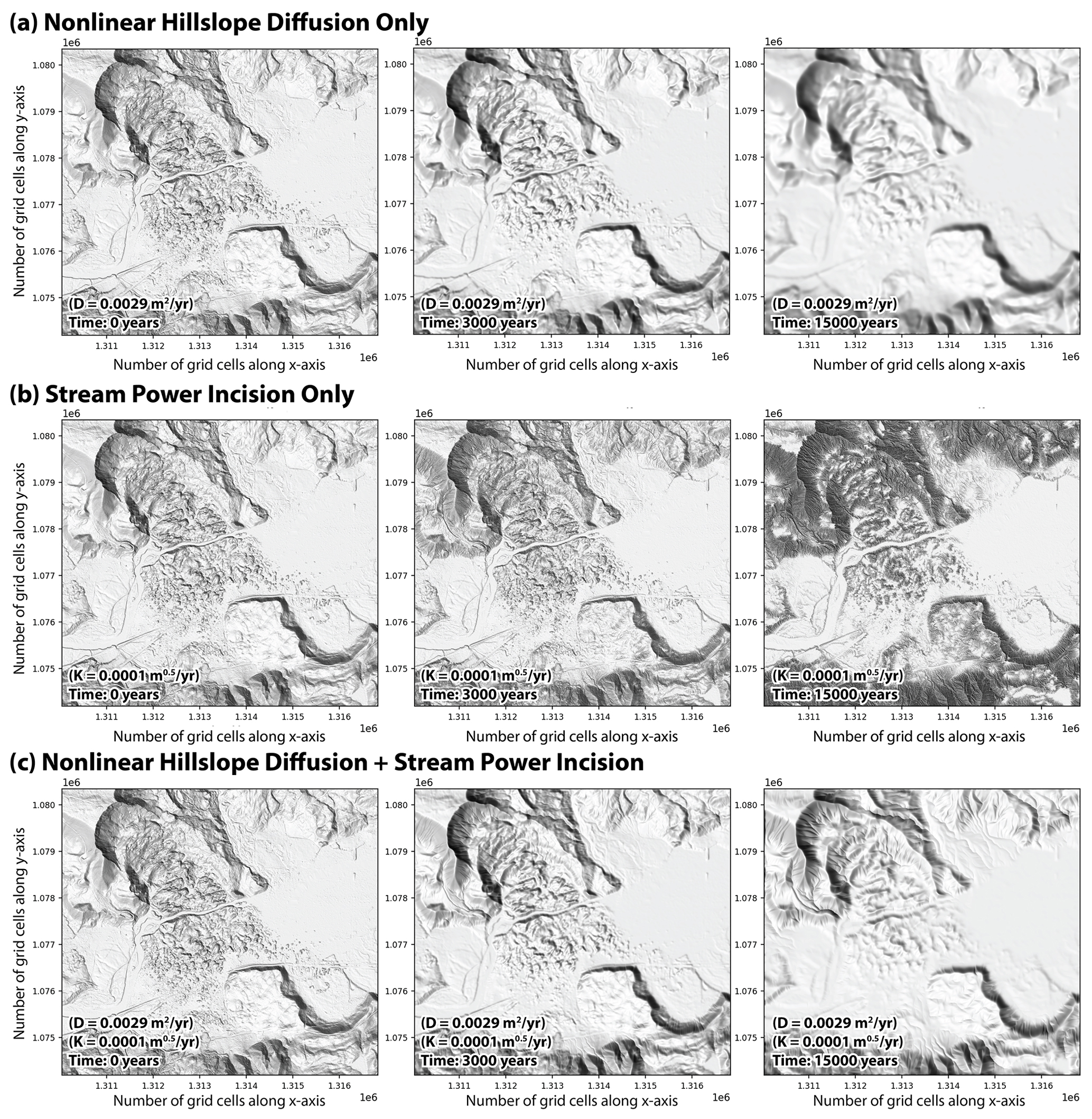
Figure 2 Hillshade maps of the 2014 Oso landslide and landscape evolution over 15 000 years predicted by models of nonlinear hillslope diffusion and stream power incision in the Landlab_simulation.ipynb.

This notebook offers a comprehensive workflow that guides users through setting up Landlab components, importing raster DTM files, running simulations, and analyzing topographic complexity on simulated landforms using pyTopoComplexity. Because Landlab primarily processes DTM data in ESRI ASCII format, the notebook converts the raster DTM files between GeoTIFF and ESRI ASCII to meet the required data formats for each toolkit. For landscape evolution modeling, users must specify values for key parameters S_c, D, and K, as well as the duration of the total simulation time and each time step (in years). The examples provided in the notebook use the 2014 Oso landslide lidar DTM data (Washington Geological Survey, 2023) to run simulations of landscape evolution over 15 000 years, activating either or both hillslope diffusion and fluvial incision components (Fig. 2). By setting D=0.0029 (m² yr⁻¹) and S_c=1.25, the hillslope-diffusion-only simulation successfully reproduces results from Booth et al. (2017) (Fig. 2a). Upon completing the Landlab simulation, users can apply the notebook's customized functions to measure topographic complexity on the simulated landscape at each time step using pyTopoComplexity, and the resulting GeoTIFF rasters can then be utilized for further geospatial analysis.

3 Case study of multiscale surface-complexity-based age estimation for landslide deposits

In regions prone to catastrophic landslides, obtaining comprehensive information on the spatial and temporal distribution of historical landslides over a large area is essential. Such data enable a more accurate quantitative assessment of landslide susceptibility for each location and help evaluate potential connections to other geohazards (earthquake shaking, wildfire, intense storm precipitation, outburst flooding from landslide dam failure, etc.). These insights are critical for effective hazard mitigation and preparedness. However, finding suitable and reliable dating constraints for every mapped landslide deposit is time-consuming and impractical. Researchers, particularly in the Pacific Northwest region of the United States, have attempted to calibrate a few types of surface complexity metrics using radiocarbon dating, and these calibrated metrics have subsequently been employed to estimate the frequency of landslides over the past thousands of years in large mapping areas (e.g., Booth et al., 2017; Herzig et al., 2024; LaHusen et al., 2020, 2016). Although previous research has demonstrated success with this approach, not all known surface complexity metrics have been thoroughly evaluated. Additionally, the optimal and acceptable spatial scales for analyzing these metrics using different approaches remain uncertain, and there is no publicly available tool to explore these questions before the development of pyTopoComplexity.

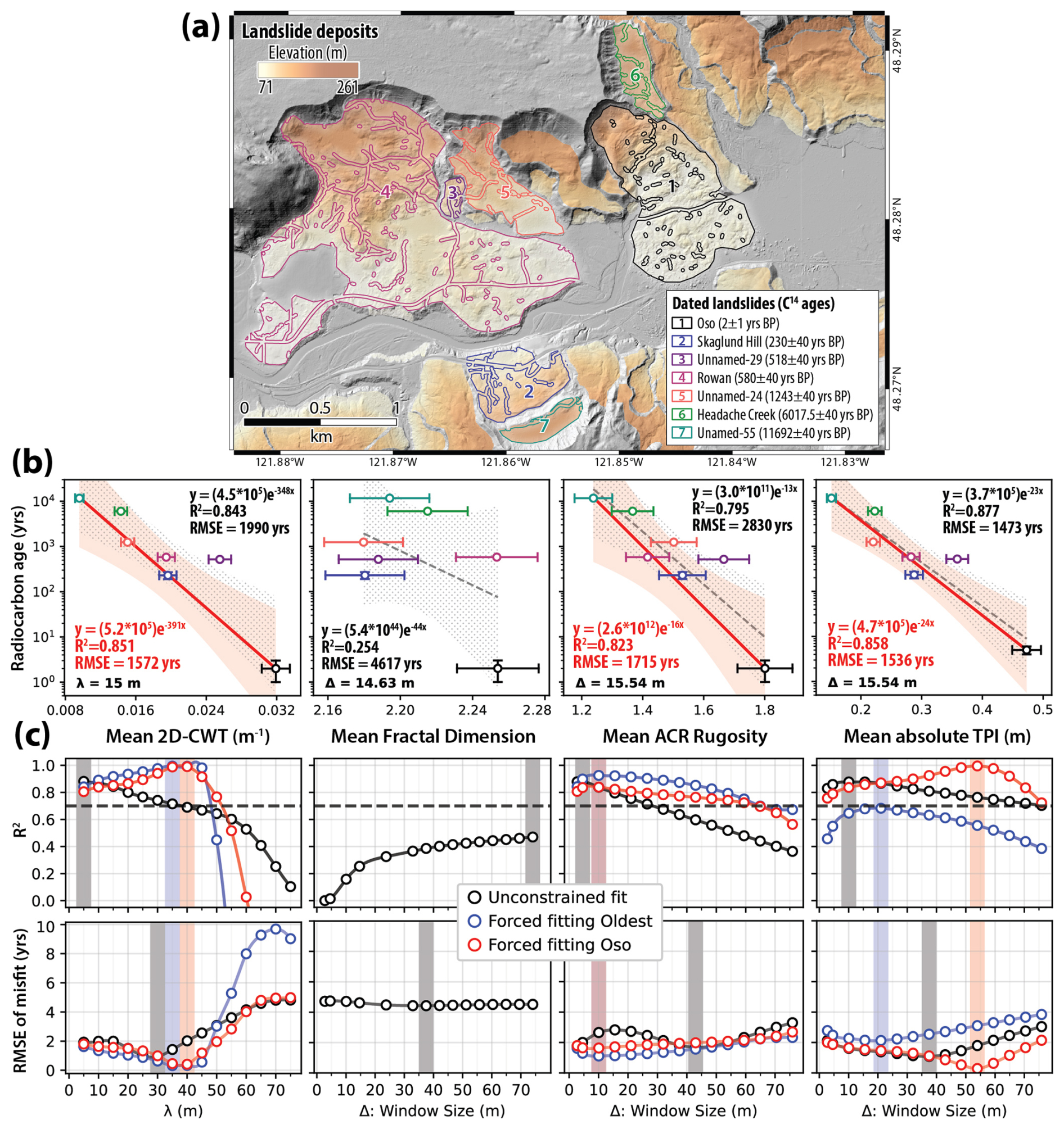
Figure 3 Evaluation of surface complexity metrics in pyTopoComplexity for estimating landslide deposit ages. (a) Seven landslides with radiocarbon ages before present (BP) from Booth et al. (2017) used in the evaluation. (b) Example of the complexity–age relationship at ∼15 m spatial scale, showing best-fit exponential-decay functions and their 95 % confidence intervals. (c) Coefficient of determination (R²) and root-mean-square error (RMSE) values between radiocarbon ages and predicted functions across spatial scales from ∼3 to ∼75 m. Best-fit curves with negative R² values are excluded. Shaded bars highlight the optimal spatial scales for age estimation for each method. See complete plots in Figs. S2–S7 and further details in the main text.

Here we present a case study applying each method from pyTopoComplexity to a published landslide inventory of the North Fork Stillaguamish River (NFSR) valley (Booth et al., 2017) in the Pacific Northwest (Fig. 3a). Our goal was to validate and evaluate the effectiveness of different metrics used to quantify topographic complexity across various scales and understand their significance to geomorphology. Complexity measurements were conducted across multiple spatial scales, ranging from ∼3 to ∼75 m, using lidar DTM data (Washington Geological Survey, 2023) for seven mapped landslides with radiocarbon age constraints from Booth et al. (2017). Areas with extreme linear depressions (e.g., gullies), flat water surfaces (e.g., ponds), and artificial modifications (e.g., roads, power lines) were excluded from the analysis, consistent with Booth et al. (2017). To evaluate the quality and predictability of the age–complexity relationship, we identified the best-fit exponential-decay functions between the dated landslide ages and the measured complexity metrics at each scale. We calculated the coefficient of determination (R²) and root-mean-square error (RMSE) between the log-transformed radiocarbon ages and the function's predictions (Figs. S2–S7 in the Supplement). In exploring these best-fit functions, we conducted standard linear regression on the log-normal scale of the mean of the seven data points and also constrained the functions to pass through either the youngest (2014 Oso landslide) or the oldest (unnamed-55 landslide, dated to ∼11 693 years before present) data points (Booth et al., 2017). In our assessment, only the best-fit functions with R²>0.7 and relatively low RMSE values were considered suitable for predicting the age of landslide deposits based on the evolution of surface complexity. The fitting with the highest R² value and/or the lowest RMSE indicates the optimal spatial scale for age–complexity correlation, likely representing the characteristic scale of geomorphic features influenced by substrate geology, landsliding mode, dominant weathering processes, and environmental forces (Booth et al., 2009, 2017; Herzig et al., 2024; LaHusen et al., 2020). Best-fit curves with negative R² values were excluded from our discussion, as they suggest an exponential-decay model does not adequately explain the data trend.

The results indicate that 2D-CWT and TPI measurements provide the most accurate predictions for the NFSR valley data, followed by the RI and then the FD (Fig. 3b and c). Curve fitting models constrained to pass through either the youngest (2014 Oso landslide) or oldest (unnamed-55 landslide) data point generally offer better predictability for landslide ages compared to unconstrained regressions. While previous studies have employed unconstrained regression (e.g., LaHusen et al., 2016; Herzig et al., 2024; Underwood, 2022) or regression constrained to the oldest dated landslide (e.g., LaHusen et al., 2020; Woodard et al., 2024), our findings demonstrate that regressions passing through the youngest landslide data point yield the highest R² values and the lowest RMSE for most complexity metrics (Figs. S2–S9 in the Supplement; see detailed comparisons in Appendix A). Among the RI types (mean of ACR-RI and conventional RI) and TPI measures (standard deviation of TPI and mean of absolute TPI values), similar predictability is observed, though the mean of ACR-RI and absolute TPI show slightly better performance (Figs. S4–S7). Notably, only the mean of the absolute C value of 2D-CWT (called “mean 2D-CWT” hereafter) and absolute values of TPI achieve best-fit functions with R²>0.98 and RMSE<500 years, highlighting them as the most effective surface complexity metrics for estimating landslide ages. This is likely because they focus on quantifying the extent and variability of surface concavity and convexity, which effectively represents the hummocky topography formed by displaced blocks and closed depressions. Conversely, the FD fails to establish a satisfactory relationship with R²>0.7. Although this method can detect scale-invariant complexity features (Huang and Turcotte, 1990; Mark and Aronson, 1984), it may not be suitable for explaining the scale-dependent smoothing trends observed in landslide-prone landscapes.

We also applied the same NFSR valley dataset to comparable analyses using other traditional topographic complexity metrics available through native and GRASS plugins in QGIS software (QGIS Development Team, 2024; GRASS Development Team, 2024). The evaluated metrics include standard deviation of slope, roughness index, total curvature, maximum curvature, absolute minimum curvature, curvedness index, unsphericity, profile curvature, plan curvature, tangential curvature, difference curvature, mean curvature (Shary, 1995; Florinsky, 2017), and the terrain ruggedness index (TRI) (Riley et al., 1999). Of these, only QGIS's TRI tool allows for multiscale assessment of surface complexity. The results indicate that most traditional metrics, except the standard deviation of plan curvature, provide acceptable predictability (R²>0.7) for the complexity–age regression (Figs. S8 and S9, Appendix A). The standard deviation of slope stood out as the best conventional metric for predicting landslide ages when the regression is constrained to pass through the oldest landslide, consistent with the findings in LaHusen et al. (2016). Nevertheless, the 2D-CWT and TPI methods from pyTopoComplexity still outperform all tested traditional metrics in terms of regression quality, showing higher R² and lower RMSE values.

From the multiscale analysis using the two most effective metrics – mean 2D-CWT and absolute values of TPI – we identified the optimal spatial scales for achieving the best-fit regression as ∼40 and ∼54 m, respectively (Fig. 3c). These characteristic scales are notably larger than those suggested in previous studies for similar analyses in the NFSR valley (∼15 m), Seattle fault zone (∼15 m), and Oregon Coast Range (∼20 m) (Booth et al., 2017; Herzig et al., 2024; LaHusen et al., 2020, 2016). This discrepancy may stem from differences in regression approaches (e.g., unconstrained regression or those constrained to pass through the oldest landslide data point therein) and the fact that earlier studies only examined spatial scales between 10 and 30 m. We also emphasize the unique capability of spectral analysis methods, such as 2D-CWT, in isolating landform signals at specific spatial scales (Perron et al., 2008b; Booth et al., 2009). This indicates that the ∼40 m optimal scale derived from the 2D-CWT method is likely more representative of the characteristic size of landform features associated with landslide deposits in the NFSR valley rather than the ∼54 m suggested by the TPI method. The exponential-decay linear relationship between landslide age and the mean 2D-CWT measure deteriorates when the spatial scale (λ) exceeds 50 m, indicating that the lengths of hummocks and depressions in these landslide deposits, influenced by substrate geology and failure mode, are generally smaller than 50 m (Figs. 3c and S2).

Although using a 40 m spatial scale for 2D-CWT analysis improves the predictability of the complexity–age regression compared to the previously used 15 m scale (Booth et al., 2017), we note that larger spatial scales can introduce greater uncertainties for smaller landslide deposits. For example, the unnamed-29 landslide, dated to ∼518 years before present, has a relatively small preserved deposit in the modern landscape (Fig. 3a). When larger-scale complexity measures are applied, results are more likely influenced by surrounding landform features. This effect is evident in our multiscale analyses, as the unnamed-29 landslide data point progressively becomes an outlier as the spatial scale increases (e.g., Fig. S2). To reduce the influence of surrounding landforms, a buffer that increases in width with the spatial scale of analysis could be imposed inside the mapped landslide deposit. However, larger buffers would result in smaller fractions of the central part of the landslide deposit being used to determine its average complexity, introducing bias or possibly eliminating the landslide from the analysis completely. Because pyTopoComplexity's multiscale analysis provides a range of acceptable spatial scales for complexity–age regression, users can select the most appropriate scale based on the quality and nature of their dataset.

4 Applications in exploring erosivity parameters in a landslide-prone landform

Landscape erosivity parameters, such as hillslope diffusivity D (Eq. 11) and channel erodibility K (Eq. 12), are critical in process geomorphology studies for understanding a landscape's susceptibility to erosion under specific environmental and geological conditions. These parameters are also essential for linking real-world observations to numerical modeling. Constraining D and K typically requires a quasi-equilibrium landscape that has undergone continuous erosion over a long period under known, stable climatic and tectonic conditions. In such cases, D can be estimated from the steady-state curvature of hillslopes or hilltops (e.g., Roering et al., 2001; Hurst et al., 2012; Struble et al., 2024), while K can be derived by inverting the longitudinal channel profile using the stream power model (e.g., Stock and Montgomery, 1999). However, in complex and unstable landscapes like the NFSR valley, which are prone to frequent landslides, estimating D and K becomes challenging. Although it is possible to approximate D based on its correlation with mean annual precipitation (Richardson et al., 2019), constraining K in a non-steady-state landscape remains impractical. To address this, we present an approach that combines landslide inventory data, modeling results, and surface complexity analysis, providing a potential solution to the problem.

We set up three modeling scenarios to explore the parameter space of D and K in the NFSR valley: (1) hillslope-diffusion-only scenario, (2) stream-power-incision-only scenario, and (3) coupled hillslope diffusion and stream power incision scenario. In each scenario, we independently vary D and K and run the simulation for 15 000 years on the 2014 Oso landslide (e.g., Fig. 2). For hillslope diffusion, we set S_c=1.25 consistent with Booth et al. (2017) and examine a range of D values from 0.00082 to 0.023 m² yr⁻¹, generally in line with measured values from the Pacific Northwest (Roering et al., 1999; Hurst et al., 2012). For stream power incision, we assume m=0.5, n=1, and Ω=0 as convention (Whipple and Tucker, 1999) and test common K values ranging from 0.000001 to 0.001 m^0.5 yr⁻¹ (Gasparini and Brandon, 2011). In the coupled scenario, we explore the parameter space by either fixing D=0.0029 m² yr⁻¹ or K=0.0001 m^0.5 yr⁻¹, while varying the other. After completing the simulations, we applied 2D-CWT analysis with pyTopoComplexity to the simulated landscapes at each time step, extracting surface complexity signals across various spatial scales and monitoring their evolution over time. Finally, we compared these simulation trends with the real-world NFSR valley data.

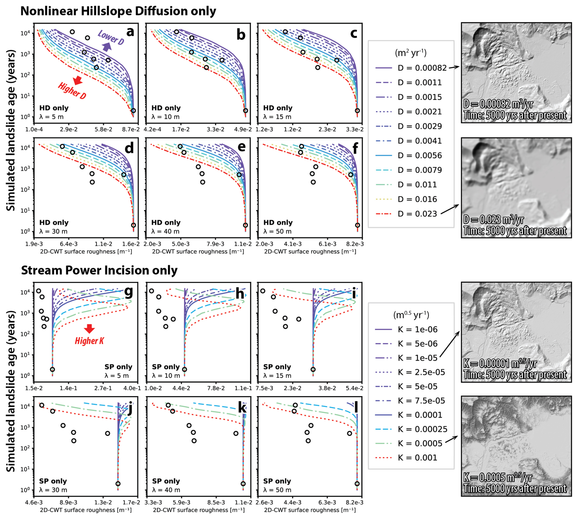
Figure 4 Changes in mean 2D-CWT surface complexity measures for the simulated landscape of the 2014 Oso landslide over a 15 000-year period, predicted by models of nonlinear hillslope diffusion (a–f) and stream power incision (g–l) in Landlab_simulation.ipynb, with varying hillslope diffusivity (D in m² yr⁻¹) and channel erodibility (K in m^0.5 yr⁻¹). Black circles represent real-world data from the seven dated landslide measurements in the NFSR valley (Fig. 3a). The right panel shows an example of simulated results at 5000 years after present. See complete simulation results in Fig. S10 in the Supplement.

The results show that, as expected, hillslope diffusion smooths the landscape over time at all spatial scales, while fluvial incision increases complexity by dissecting the terrain (Fig. 4). In the hillslope-diffusion-only scenario, higher D values accelerate the reduction of surface complexity, with smaller-scale (<15 m) complexity diminishing more quickly and showing greater sensitivity to changes in D (Figs. 4a, b and S10a). In the stream-power-incision-only scenario, channelization significantly increases surface complexity, particularly at smaller scales (<30 m) (Figs. 4g–i and S10b). Regardless of the value of K, there exists a consistent maximum complexity value at every spatial scale. Simulations employing higher K values attain this maximum value more rapidly in time. Once this time threshold is exceeded, surface complexity declines rapidly as the entire topography of the landslide deposit is progressively eroded by the retreating headwaters and drainage systems.

By comparing real-world NFSR landslide data to these scenarios running with separate models, we assure that the fluvial incision process alone cannot produce the natural smoothing trend of the post-landslide landscape recovery. While the hillslope-diffusion-only scenario can generate an increasingly smoothed landscape over time, no single run using a constant D value can replicate the observed exponential-decay relationship between surface complexity and landslide age across the entire real-world dataset. For a given D, the non-linear diffusion model tends to underpredict the reduction rate of surface complexity during the early stages of landscape recovery following a catastrophic landslide. The timescale for this reduction appears to be scale-dependent: smaller-scale features (e.g., ∼5–15 m) experience underprediction within 10¹ to 10² years (Fig. 4a–c), while larger features (e.g., >25 m) are affected over a longer period of 10² to 10³ years (Fig. 4d–f). After 10³ to 10⁴ years, the model tends to over-smooth small-scale features. These observations suggest the need for a mechanism that accelerates complexity reduction during the initial recovery phase, a roughening process to counteract over-smoothing by diffusion over longer timescales, and an explanation for the observed scale dependency.

Since the position of the NFSR river bed at the toes of the studied landslides remained relatively stationary during the Holocene (LaHusen et al., 2016), the rate of landform smoothing on these landslide deposits is unlikely to have been affected by changes in the local base level within the time frame of our investigation (the last ∼15 000 years). Thus, the observed initial acceleration of smoothing can be attributed to higher in situ diffusivity D, reflecting increased hillslope sediment transport efficiency at the beginning of landscape recovery when loose and unconsolidated materials covered the barren landslide deposits (Booth et al., 2017). The reactivation of landslides, which commonly occurs in the early stages of recovery before the deposits settle, could also offer an additional roughening process over shorter time frames. An example is the Hazel landslide in the NFSR valley, where hillslope movement persisted for decades before the Oso landslide occurred in the same area (Miller and Sias, 1998). However, since the natural reestablishment of vegetation and soil development typically spans 10¹ to 10² years (e.g., Fu et al., 2017; Kennedy et al., 2012; Seidl et al., 2014; White et al., 2022; Russell and Michels, 2011), other roughening mechanisms are necessary to sustain surface complexity over longer periods. One possible factor that maintains topographic complexity after revegetation is tree throw, which can continuously create new small-scale (∼7.5 m) roughening features over decadal time frames (Roering et al., 2010). Long-term climate change could be another important factor. In the Pacific Northwest, research suggests a drier climate from approximately 10 000 to 6000 years ago, followed by a transition to wetter conditions similar to those of the present day in the last ∼6000 years (Leopold et al., 1982; Brubaker, 1991). This climate shift implies that hillslope diffusivity may have increased over the Holocene as precipitation levels rose (Richardson et al., 2019), potentially explaining the complexity–age patterns observed in smaller-scale features.

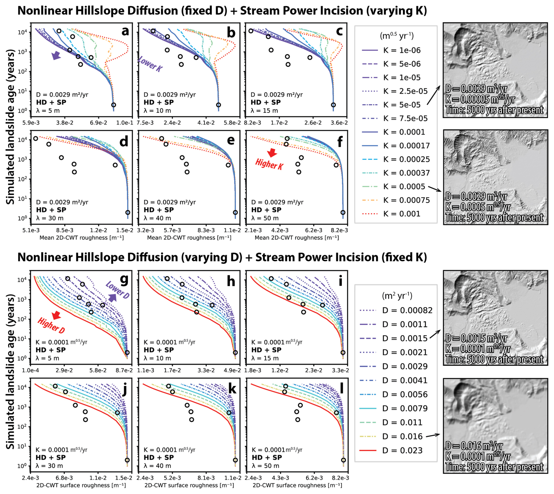
Figure 5 Changes in mean 2D-CWT surface complexity measures for the simulated landscape of the 2014 Oso landslide over a 15 000-year period, predicted by coupled models of nonlinear hillslope diffusion and stream power incision in Landlab_simulation.ipynb. (a–f) Simulations with a fixed D=0.0029 m² yr⁻¹ and varying channel erodibility (K in m^0.5 yr⁻¹). (g–l) Simulations with a fixed K=0.0001 m^0.5 yr⁻¹ and varying D in m² yr⁻¹. Black circles represent real-world data from the seven dated landslide measurements in the NFSR valley (Fig. 3a). The right panel shows an example of simulated results at 5000 years after present. See complete simulation results in Fig. S11.

Another possibility, without changing D over a longer timescale, is to consider the combined effects of channel incision (which roughens the landscape) and hillslope diffusion (which smooths it). In our modeling scenario with these coupled processes, we produce a complexity–age trend that more closely matches the observed NFSR valley data at smaller spatial scales while keeping D and K constant (Figs. 5 and S11 in the Supplement). For the 5 m scale, the NFSR valley data are roughly bounded by modeled curves with K values between 0.0001 and 0.00037 m^0.5 yr⁻¹ and D values between 0.0011 and 0.0041 m² yr⁻¹ (Fig. 5a and g). Comparing the simulation results between fixed D and fixed K indicates that the pattern of complexity reduction is more sensitive to variations in K. Only a narrow range of K values for a given D results in the observed exponential-decay relationship between surface complexity and landslide age, suggesting a natural scaling relationship between D and K for a given environmental and geological setting. This finding is consistent with observations from steady-state landforms, where the length scale (i.e., the scale of landform complexity) between evenly spaced channels and ridgelines is governed by a specific constant $D/K$ ratio (Perron et al., 2008a, 2009), reflecting the balance and self-regulation between diffusive smoothing and channel dissection. If this model-coupling hypothesis holds, it suggests that the time required for a landscape to recover from a rugged landslide surface to its background complexity level may be longer than previously estimated using diffusion-only simulations (cf. Woodard et al., 2024) due to the prolonged resistance to smoothing by continuous channel incision.

While our estimated D range with coupled models at 5 m generally aligns with the estimation of diffusion-only modeling from Booth et al. (2017) at 15 m scale, we note that we are unable to reproduce the same bracketed D value range using 15 m scale complexity measurements (Figs. 4c and 5a, g). In fact, the complexity reduction trend varies across different spatial scales in all of our simulation scenarios, which is different from the consistent exponential-decay pattern in the real-world observation across the scales (at least for 5 to 50 m in 2D-CWT analysis) (Figs. S2, S10, and S11). Specifically, for the diffusion-only models, larger values of D better match the observed landslide age–complexity data as the spatial scale increases (Fig. 4d–f). The D values most consistent with those that have been independently inferred from hilltop curvature in the Pacific Northwest only fit our landslide data reasonably well when surface complexity is quantified at relatively short length scales (e.g., <15 m) (Figs. 4a, b and 5g, h). We suggest that this is because D values are typically inferred from hilltop curvature with smoothed lidar data at similarly short length scales (e.g., Hurst et al., 2012; Struble et al., 2024).

When stream power incision is introduced into the model, it roughens the landscape at smaller scales through channel dissection (Figs. 2b, c and 3b). This indicates that a higher initial diffusivity (D), as previously discussed, may still be necessary to counterbalance the complex landforms created by channel incision within the first 10¹ to 10² years following a landslide event. On the other hand, the modeling bias toward higher complexity at larger spatial scales (Fig. 4d–f) suggests that the intricacies of natural behavior in landslide-prone landscapes cannot be fully captured using simple models of nonlinear diffusion (Eqs. 10 and 11) and stream power incision (Eq. 12) with constant erosivity parameters. The deviation between the simulation results between the coupled modeling scenario and real-world data at a larger spatial scale, particularly at the time frame of 10² to 10³ years, may reflect that D and K values are scale-dependent. To approach the observed real-world data trend using these simple models, it requires a much higher D (and/or a smaller K) to explain the reduction rate of the landform features with larger length scale (Fig. 5). It seems plausible because the landslides produce a vast range of materials at different length scales, and the mechanical properties and mobility of these materials are likely size-dependent (Collins and Reid, 2019; Wartman et al., 2016). Large, sharp, and fractured landslide blocks may be more susceptible to rapid hillslope erosion and smoothing, requiring a higher D to account for the age–complexity relationship at larger scales. In contrast, the hillslope erosion rates for smaller, looser particles are more likely limited by local variability in topography, hydrology, lithology, and bioturbation, reflecting a smaller D.

Although these simple modeling tests presented in this short communication do not fully resolve all observed geomorphic questions in the NFSR valley, we emphasize the potential of studying topographic complexity in landslide-prone terrains to gain insights into the fundamental erosivity parameters that drive landscape evolution at various spatial scales. The integrated approach of Landlab and pyTopoComplexity offers a quantitative method for evaluating the efficiency of landform adjustments to erosion and understanding dominant surface processes. Additionally, Landlab provides several other components with advanced erosion models that account for complex processes, such as variability in soil production rates on hillslopes, mass wasting, stream power incision thresholds (e.g., in Eq. 12), and sediment transport and cover effects in channels (e.g., Barnhart et al., 2020; Hobley et al., 2017; Shobe et al., 2017; Campforts et al., 2022), which were not included in our simulations. In our notebook Landlab_simulation.ipynb, users can directly import those components from Landlab and explore landscape evolution through the lens of topographic complexity measures.

5 Conclusions

pyTopoComplexity is an open-source software package designed for efficiently quantifying topographic complexity using advanced methods such as two-dimensional continuous wavelet transform analysis, fractal dimension estimation, rugosity index, and terrain position index calculations. By bridging the gap between traditional terrain analysis tools and modern quantitative geomorphology, it offers users robust and reproducible measures of surface complexity across multiple spatial scales, generating insights across research fields, including geology, geomorphology, geography, ecology, and oceanography.

A case study in the North Fork Stillaguamish River valley, WA, USA, showcases software capability to accurately assess the morphometric properties of landslide deposits, revealing characteristic landform scales and enhancing our understanding of geomorphic processes. The integrated approach using the notebook Landlab_simulation.ipynb combines dated landslide inventories, Landlab's landscape evolution modeling components, and multiscale topographic complexity analysis, demonstrating pyTopoComplexity's effectiveness in linking real-world data with simulation-based insights. This framework allows users to explore landscape recovery rates and mechanisms by estimating in situ hillslope diffusivity (D) and channel erodibility (K), critical factors in understanding landscape evolution and response to disturbances. Leveraging the modular flexibility of Landlab, users can also integrate other erosion models to investigate how different processes shape the dynamic evolution of topographic complexity in response to natural forces and catastrophic geohazard events like landslides.

Appendix A

Table A1 Comparisons among the tested surface complexity metrics. See complete testing results in Figs. S2–S9.

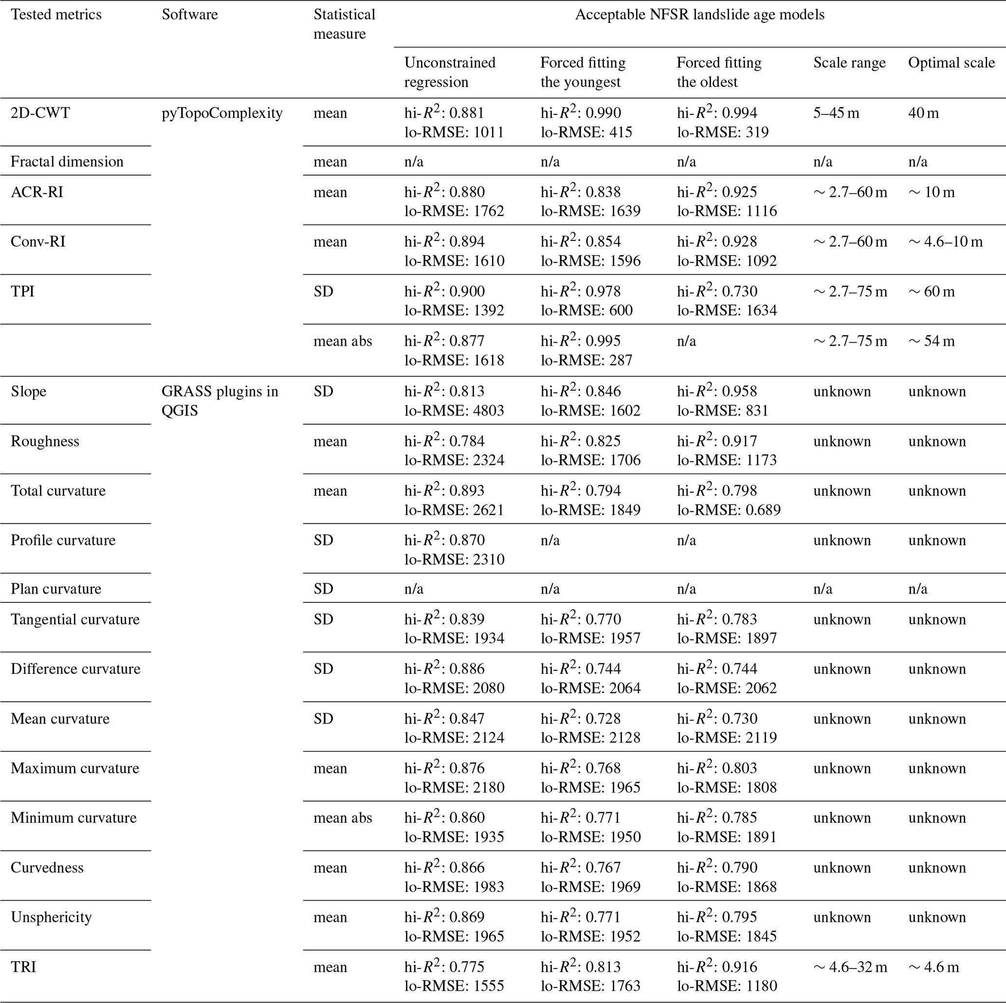
SD: standard deviation; abs: absolute values; 2D-CWT: wavelet coefficient (C) of two-dimensional continuous wavelet transform analysis; ACR-RI: arc–chord ratio rugosity index; Conv-RI: conventional rugosity index; TPI: terrain position index; TRI: terrain ruggedness index; n/a: unavailable because there is no strong relationship between depositional age and that complexity metric; unknown: unknown due to the lack of multiscale analysis capability in the GRASS plugins; NFSR: North Fork Stillaguamish River; hi-R²: the highest coefficient of determination of the linear regression (higher means better predictability); lo-RMSE: the lowest root-mean-square error (in years) of the linear regression (lower means better predictability).

Appendix B: Notation

A	Upstream drainage area [m2]
Ac	Contoured area (i.e., true geometric surface area) within a square window of Δ2 [m2]
Ap	Planimetric area within a square window of Δ2 [m2]
C	Resultant wavelet coefficient of 2D-CWT analysis [m−1]
D	Hillslope diffusivity [m2 yr−1]
E	Erosion rate [m yr−1]
K	Channel erodibility coefficient (units vary with m and n) [m0.5 yr−1 when m=0.5 and n=1]
m	Exponent of drainage area (A) in stream power equation
N	Number of terms in the Taylor expansion of hillslope sediment flux equation
n	Exponent of channel slope (Ssp) in stream power equation
p,P	Lag distances ($p=\mathrm{1},\mathrm{\dots },P$) along the one-dimensional topological profile for variogram analysis [m]
qs	Two-dimensional vector of the sediment flux per unit slope width at the surface
r,R	Length steps ($r=\mathrm{1},\mathrm{\dots },R$) along the one-dimensional topological profile for variogram analysis [m]
Sc	Asymptotic maximum hillslope gradient
Shd	Two-dimensional vector of topographic downslope gradient at each grid point
Shd	Hillslope gradient (i.e., the magnitude of Shd)
Ssp	Channel slope
s	A wavelet-scale parameter for 2D-CWT analysis
t	Time [year(s)]
x	Distance in easting direction of each grid cell in the DEM raster [m]
y	Distance in northing direction of each grid cell in the DEM raster [m]
z	Distance in up direction (i.e., elevation) of each grid cell in the DEM raster [m]
$\stackrel{\mathrm{‾}}{z_{\text{nb}}}$	Mean elevation of grid cells surrounding each grid point within a square window of Δ2 [m]
α	Coefficient of the ideal power-law one-dimensional variogram function
β	Exponent of the ideal power-law one-dimensional variogram function
γ1	One-dimensional variogram function
Δ	Designated window size for spatial analysis (number of grids times δ) [m]
δ	Grid spacing of the DEM raster [m]
λ	Fourier wavelength of the wavelet function ψ [m]
ψ	Mexican hat wavelet (i.e., 2D Ricker or Marr wavelet) function
Ω	Threshold of channel erosion [m yr−1]