Modeling active layer thickness in permafrost rock walls based on an analytical solution of the heat transport equation, Kitzsteinhorn, Hohe Tauern Range, Austria

The active layer thickness (ALT) refers to the seasonal thaw depth of a permafrost body and in high alpine environments represents an essential parameter for natural hazard analysis. The aim of this study is to model ALT based on bedrock temperature data measured in four shallow boreholes (SBs, 0.1 m deep) in the summit region of the Kitzsteinhorn (Hohe Tauern Range, Austria, Europe). We set up our heat flow model with temperature data (2016–2021) from a 30 m deep borehole (DB) drilled into bedrock at the Kitzsteinhorn north face. For modeling purposes, we assume one-dimensional conductive heat flow and present an analytical solution of the heat transport equation through sinusoidal temperature waves resulting from seasonal temperature oscillations (damping depth method). The model approach is considered successful: in the validation period (2019–2021), modeled and measured ALT differed by only 0.1 ± 0.1 m, with a root mean square error (RMSE) of 0.13 m. We then applied the DB-calibrated model to four SBs and found that the modeled seasonal ALT maximum ranged between 2.5 m (SB 2) and 10.6 m (SB 1) in the observation period (2013–2021). Due to small differences in altitude (∼200 m) within the study area, slope aspect had the strongest impact on ALT. To project future ALT deepening due to global warming, we integrated IPCC climate scenarios SSP1-2.6 and SSP5-8.5 into our model. By mid-century (∼2050), ALT is expected to increase by 48 % at SB 2 and by 62 % at DB under scenario SSP1-2.6 (56 % and 128 % under scenario SSP5-8.5), while permafrost will no longer be present at SB 1, SB 3, and SB 4. By the end of the century (∼2100), permafrost will only remain under scenario SSP1-2.6 with an ALT increase of 51 % at SB 2 and of 69 % at DB.

1 Introduction

Permafrost is defined as ground (soil or rock and the water contained therein) that remains below 0 °C for at least two consecutive years (Harris et al., 1988) and is warming on a global scale (Biskaborn et al., 2019). In steep environments, such as the European Alps, warming-induced permafrost degradation is capable of destabilizing slopes and rock walls (Gruber et al., 2004; Gude and Barsch, 2005; Fischer et al., 2006; Gruber and Haeberli, 2007; Krautblatter et al., 2013). Consequently, permafrost degradation is considered as one of the main causes for natural hazards in high-alpine areas and is expected to play a significant role in triggering a wide spectrum of mass movements ranging from debris flows (Stoffel et al., 2014), to medium-scale rockfalls (Legay et al., 2021) to large-scale rock avalanches such as recently witnessed at the Piz Cengalo at the Swiss-Italian border (Walter et al., 2020) or in 2023 at the Fluchthorn (Austria). In general, European mountain permafrost is characterized by ground temperatures just slightly below the freezing point (warm permafrost), and as a result is highly climate sensitive (Harris et al., 2009). Direct ground temperature measurements have shown, in some parts very fast, warming in the European Alps within recent decades (Etzelmüller et al., 2020).

The active layer thickness (ALT) refers to the ground's thaw depth during the summer season. The seasonally thawed active layer is not permafrost by definition, but is a key parameter of permafrost bodies (Harris et al., 1988; Michaelides et al., 2019). In periglacial landscapes, geomorphological, ecological, hydrological, and pedological processes take place almost exclusively within the active layer (Hinzman et al., 1991; Harris et al., 2009). ALT evolution over time thus represents a critical variable for hazard management and prevention, but also to accurately quantify greenhouse gas release from permafrost soils (Miner et al., 2022). Microbial activity and the decay of organic matter is restricted to the active layer. Consequently, ALT data provide required information to investigate carbon–climate feedbacks in earth system models (Mishra et al., 2017). They are also required for land-use planning and construction on permafrost to warrant foundation stability and to avoid infrastructure damage (Hjort et al., 2022). In high-mountain regions exceptional rockfall activity has been observed as a direct response to the thickening or new formation of the active layer during hot summers, which potentially exposes deep-seated failure planes to positive temperatures (e.g., Allen and Huggel, 2013; Ravanel et al., 2017). Due to its broad relevance across many disciplines, the Global Climate Observing System (GCOS, 2021) has recognized the ALT as an “essential climate variable” (ECV), i.e., as a parameter that critically contributes to the characterization of Earth's climate (GCOS, 2021). ALT data are collected in a global database (GTN-P – Global Terrestrial Network for Permafrost; Biskaborn et al., 2015), which reveals a worldwide trend towards ALT deepening (Biskaborn et al., 2019; Streletskiy et al., 2020; Kaverin et al., 2021).

Complex mountain topography (altitude, slope aspect, inclination) significantly modifies the amount of incoming solar radiation received by the ground surface. It thus has a pronounced effect on surface net energy input and leads to a high spatial variability of subsurface temperatures (Haeberli et al., 2010; Gubler et al., 2011). As a result, ALT varies strongly at the same elevation, ranging from a few meters to more than 10 m (PERMOS, 2023). ALT can be precisely recorded through temperature measurements in deep boreholes. High-alpine drilling works are, however, technically challenging, expensive, and time-consuming, and only provide point recordings with limited spatial representation. The implementation of shallow boreholes (SBs) to record near-surface temperature (e.g., at 0.1 m depth), however, is simpler and allows significantly more measurement points (Hartmeyer et al., 2012), yet provides no direct ALT recordings due to an insufficient penetration depth. In this study, we used near-surface temperature data (0.1 m depth), which is widely available in permafrost regions, to simulate ALT based on the heat transport equation.

A comprehensive overview of various permafrost heat flow modeling approaches is provided in the review paper by Riseborough et al. (2008). So far, numerous studies of lowland (e.g., Burn and Zhang, 2009; Etzelmüller et al., 2011) and mountain permafrost (e.g., Engelhardt et al., 2010; Hipp et al., 2012) have simulated heat flow and ALT using one-dimensional (1D) numerical models, which are well suited to handle heterogenous material properties. For the first time, we present here an analytical solution to the heat transport equation for 1D ALT modeling in permafrost-affected rock walls (borehole scale). Analytical solutions provide a direct mathematical description of the relationship between variables and therefore offer a concise, process-based understanding of how (modified) input parameters impact the studied system. This is of particular relevance in global-warming-related sensitivity analyses to estimate the extent to which changes in input parameters (e.g., rising temperatures) impact the result of a model without the need for extensive simulations. Following De Vries (1963), we analytically solved the heat transport equation through sinusoidal thermal waves that propagate into the subsurface. A 6 year dataset from a 30 m deep borehole (DB) at the Kitzsteinhorn (Austria) served as a data base for model calibration and validation. The model was then used to simulate present-day ALT at four SBs (0.1 m deep) located in the same study area, assuming identical thermal properties due to highly similar bedrock properties. In addition, we integrated IPCC (Intergovernmental Panel on Climate Change) climate projections (IPCC, 2023) into our model to simulate the ALT for the middle and the end of the century. The new approach was applied to a single mountain (Kitzsteinhorn summit pyramid), but is well suited to modeling ALT at larger scales in steep bedrock environments.

2 Study area

The Kitzsteinhorn is part of the Hohe Tauern mountain range in the central Eastern Alps (Austria). The highest point is at 3203 m a.s.l. ($\mathrm{47}\mathit{°}{\mathrm{11}}^{\prime }{\mathrm{17}}^{\prime \prime }$ N, $\mathrm{12}\mathit{°}{\mathrm{41}}^{\prime }{\mathrm{15}}^{\prime \prime }$ E). Because of the relative singularity of the mountain massif and a pyramidal summit structure, the study area is well suited to investigate the influence of slope aspect and elevation on ground temperature. The climate at the Kitzsteinhorn, which is located just north of the main alpine ridge, is characterized by humid, high-alpine weather conditions (Otto et al., 2012). In the vicinity of the study area (<2 km), three weather stations are located at different altitudes. The stations at Glacier Plateau (GP) and Kammerscharte (KS) are closest to the boreholes investigated in this study, and annual air temperatures at these two stations are highly similar (Table 1). Minimum temperatures occur in January and February, maximum temperatures in July and August.

Table 1 Weather data from three nearby (<2 km) weather stations: Alpincenter (AC), Gletscherplateau (GP), and Kammerscharte (KS). MAAT: mean annual air temperature (period 2011–2021).

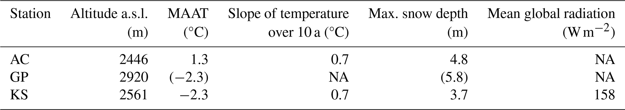
Values for GP are given in brackets due to gaps in the period 2018–2020; NA: not available.

In the study area, permafrost distribution was simulated using the empirical–statistical model “Permakart 3.0”, which estimates permafrost probability using a topo-climatic key for the Hohe Tauern mountain range (Schrott et al., 2012). Based on this simulation, permafrost can be expected with a high probability (>75 %) for north-facing rock wall sections in the summit region. In contrast, no significant permafrost occurrence is expected on the south-facing mountain slopes (Fig. 1).

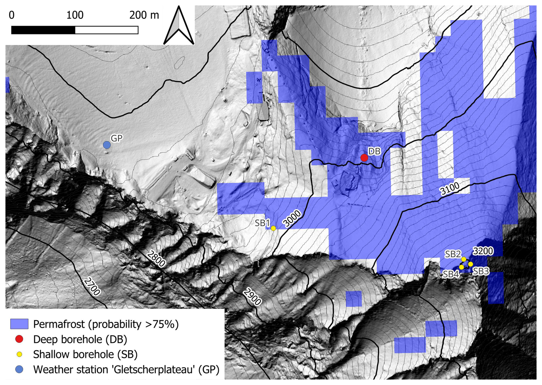
Figure 1 Borehole locations for temperature logging in the Kitzsteinhorn study area. The thermal model used to estimate active layer thickness (ALT) was calibrated and validated on the deep borehole (DB). Permafrost probability, derived from the empirical–statistical model “Permakart 3.0” (Schrott et al., 2012), is high for north-facing rock slope sections in the summit region.

Most of the bedrock in the study area is made up of gray-blue (freshly fractured) and yellow-brown (with incipient weathering) calcareous mica schist (Krainer, 2005). Tectonic stress in combination with intense physical weathering has led to the formation of joints with large apertures (Hartmeyer et al., 2012). Optical borehole imaging carried out at the deep borehole immediately after drilling showed joint size apertures of a few millimeters up to several centimeters (usually <5 cm) in the first couple of meters of the borehole. With increasing depth, the calcareous mica schist becomes more compact. Due to the schistosity, dipping steeply (∼45°) towards north, the rock has an anisotropy for water and heat transport. To quantify bedrock pore volume, seven core samples from the study area (Fig. D1) were weighed after 6 weeks of water saturation and after drying at 105 °C over 24 h to achieve a constant weight. The resulting effective porosity (ϕ_eff), which includes only the hydraulically connected pores (Sass, 2005) ranged from 0.3 %–0.4 % (Table D1). Furthermore, the sum of connected and unconnected pores was quantified by determining the samples' matrix volume (V_m) with a helium pycnometer (AccuPyc II, Micromeritics Instrument Corp., USA). The derived (total) porosity (ϕ) ranged from 0.4 %–1.0 %.

The study area hosts a long-term geoscientific monitoring project (“Open-Air-Lab Kitzsteinhorn”) which was initiated in 2010 and investigates the impact of global warming on permafrost thaw and rock stability based on a combination of subsurface, surface, and atmospheric measurements (Hartmeyer et al., 2012, 2020a, b). The present study is based on the existing research infrastructure and uses bedrock temperature data from a 30 m deep borehole (DB) and four SBs (0.1 m deep; Table 2, Fig. 1). DB is situated approximately 50 m below the local cable car top station in a thermally undisturbed, north-facing rock slope section with a 45° average gradient. The SBs were selected based on slope aspect, altitude, accessibility, and data availability (numerous DB sites in the area could not be used for the present study due to significant data gaps related to lightning strike damage). SB 2 (NW), SB 3 (ENE), and SB 4 (SE) are located in the immediate vicinity of the Kitzsteinhorn summit. Due to their almost identical altitude (∼3200 m a.s.l.) this SB trio is well suited to specifically study the impact of slope aspect on ALT. SB 1 (similar slope aspect to SB 2) and DB are situated ∼200 vertical meters below SB 2–4 and represent an interesting contrast to investigate altitudinal effects.

Table 2 Borehole locations and temperature logging depths.

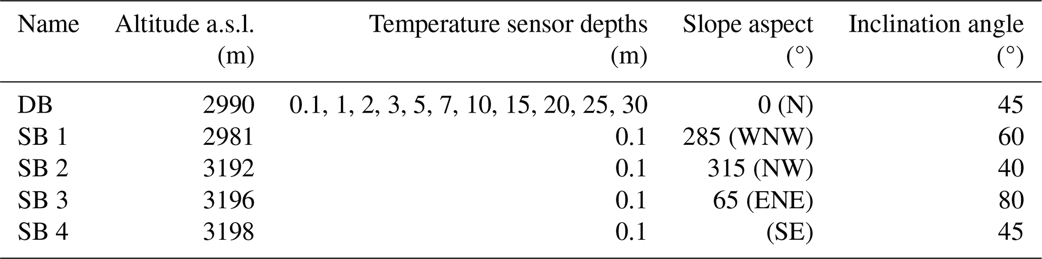
Altitude a.s.l. refers to the borehole mouth. The boreholes were drilled perpendicular to the local inclination angle (DB: deep borehole; SB: shallow borehole).

3 Material and methods

3.1 Temperature logging and data processing

The deep borehole (DB) was drilled with air rotary drilling equipment (diameter 90 mm) to a depth of 30 m (Fig. 2a and b). The borehole was then instrumented with an innovative temperature measurement system consisting of a PVC casing with brass segments at the designated sensor depths (Hartmeyer et al., 2012). Upon insertion of the thermistor chain, all temperature sensors establish direct contact with the casing's brass segments. Due to the high thermal conductivity of the brass segments (∼110 $\mathrm{W}{\mathrm{m}}^{-\mathrm{1}}{\mathrm{K}}^{-\mathrm{1}}$) this setup enables excellent thermal coupling between the temperature sensors and the surrounding bedrock. The annulus was filled with concrete to avoid water entry and potential ice formation. This most likely has a negligible effect on heat conduction between temperature sensors and ambient rock for the following reasons: (i) due to the 45° drilling angle the entire casing rests on the borehole “floor,” the bottom side of the casing is therefore in permanent physical contact with the surrounding bedrock; (ii) thermal conductivity differs only slightly between concrete (∼2 $\mathrm{W}{\mathrm{m}}^{-\mathrm{1}}{\mathrm{K}}^{-\mathrm{1}}$) and schists (∼3 $\mathrm{W}{\mathrm{m}}^{-\mathrm{1}}{\mathrm{K}}^{-\mathrm{1}}$; Talebi et al., 2020; Balkan et al., 2017). Temperature inside the DB is measured with high-precision Pt100 thermistors with an accuracy of ±0.03 °C between −50 and 400 °C (Platinum Resistance Temperature Detector L220, $\mathrm{1}/\mathrm{10}$ B, Heraeus Sensor Technology^®, DE).

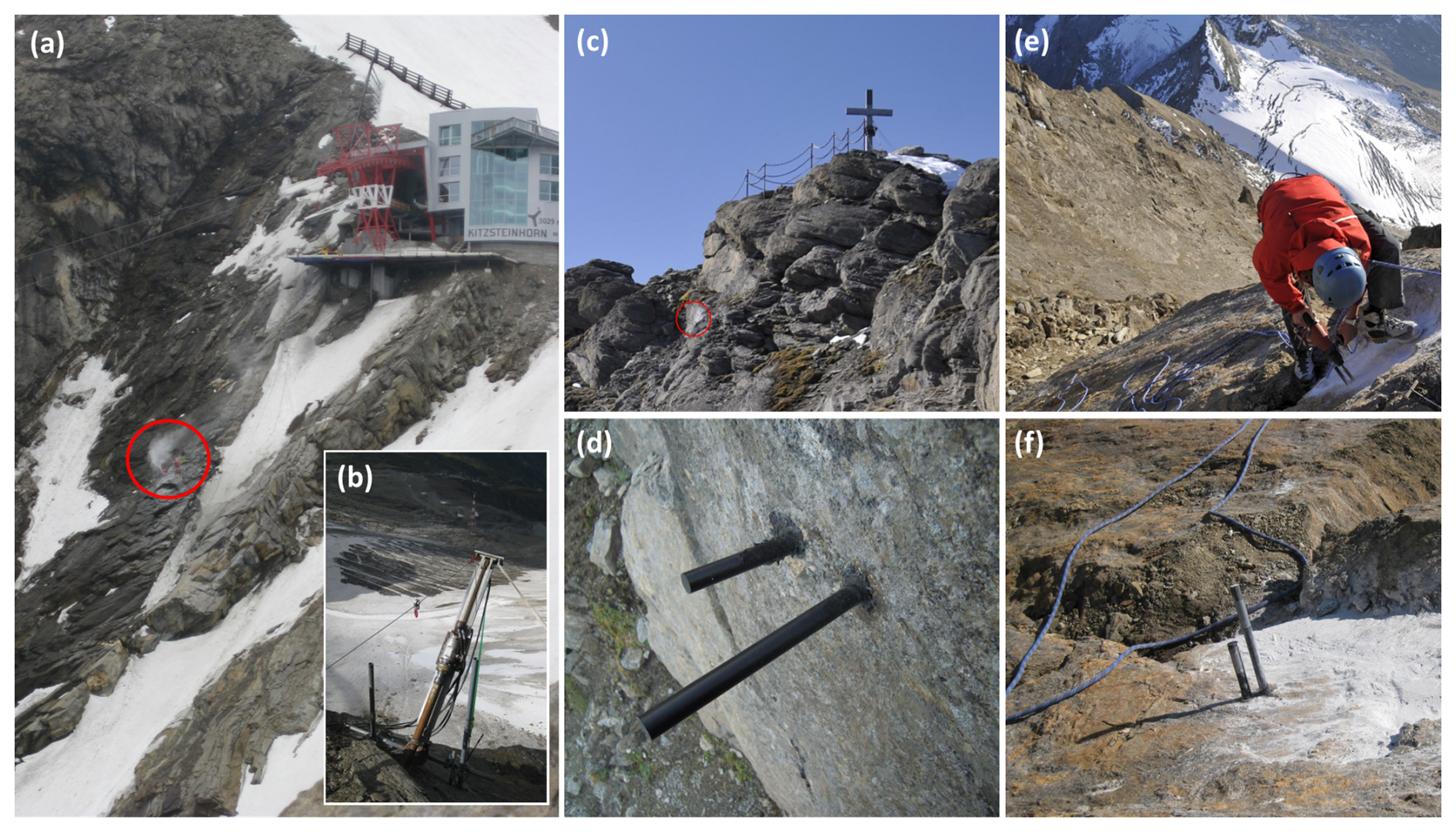
Figure 2 (a) Section of the Kitzsteinhorn north face, with the red circle marking the DB drilling site (7 July 2011). (b) Drilling equipment at DB (17 August 2011). (c) Location of SB 3 below the Kitzsteinhorn summit, with the red circle marking the SB 3 drilling site (6 October 2011). (d) Close-up of SB 3 (31 July 2013). (e) Drilling works at SB 4 (5 October 2011). (f) Close-up of SB 4 (5 October 2011). (All photos taken by Ingo Hartmeyer.)

In addition to the DB, we used ground temperature data measured in four shallow bedrock boreholes (SBs), which were drilled to a depth of 0.1 m (diameter 18 mm). All SB locations are characterized by (i) a compact rock mass without significant joints, (ii) a uniform microtopography (“clean” slope aspect), and (iii) the absence of an unconsolidated sediment cover (Fig. 2). The temperature sensors used (iButton^®, DS1922L, Maxim Integrated Products^®, USA) were glued to PVC rods (17 mm diameter) and inserted into the SBs. After insertion, the borehole entrance was sealed watertight with silicone. The sensors consist of a button cell (steel housing) with an integrated computer chip, real-time clock, and temperature sensor with an accuracy of ±0.5 °C within the temperature range −10 to 65 °C. Extensive empirical testing with iButtons^®, however, yielded an absolute sensor accuracy of ±0.21 °C, underlining their suitability for high-quality thermal monitoring (Hubbart et al., 2005).

For model development (calibration and validation), DB daily mean temperature was used for the period 1 January 2016 to 31 December 2021. Daily mean values were determined based on 12 measurement points per day. Temperature data were spline-interpolated (Δz=10 cm) for better depth resolution between measurements. Due to polynomial adjustments of the spline interpolation, positive interpolation values (<0.1 °C) between two negative measurement values occurred in 39 cases. Since these interpolation values were not realistic, they were set to 0 °C. The depth z (m) and time t (d) of the year where temperature T(z,t) was above 0 °C were estimated from the measured and interpolated depth- and time-dependent temperature data; daily thaw depths were subsequently derived. Model applications at the SBs were based on temperature records in the period 1 January 2012 to 31 December 2021; however, large data gaps existed in some cases. Temperature in the SBs was recorded every 3 h (hourly measurements could not be implemented due to limited memory space on the iButton^®) and resulted in eight measurement points per day for daily mean temperature calculations. (Note that throughout the study the mathematical plus-minus sign (±) between two values stands for standard deviation.)

3.2 Thermal modeling

Conduction was assumed to be the only transport mechanism of heat flow, thus neglecting convection and latent heat release. Conductive heat transport can be described by the heat transport equation, which describes temperature change as a function of space and time (Williams and Smith, 1993):

$$\begin{array}{}\text{(1)}& {\displaystyle \frac{\partial T}{\partial t}}=\mathit{\alpha }{\displaystyle \frac{{\partial }^{\mathrm{2}}T}{\partial z^{\mathrm{2}}}},\end{array}$$

with $\partial T/\partial t$ being the first derivative with respect to time (Δt (s)), α the thermal diffusivity (m² s⁻¹), and ${\partial }^{\mathrm{2}}T/\partial z^{\mathrm{2}}$ the second derivative with respect to position in terms of depth (Δz (m)). The thermal diffusivity α (m² s⁻¹) is defined as the quotient of the thermal conductivity λ ($\mathrm{J}{\mathrm{s}}^{-\mathrm{1}}{\mathrm{m}}^{-\mathrm{1}}\mathrm{°}{\mathrm{C}}^{-\mathrm{1}}$) and the specific volumetric heat capacity C_V ($\mathrm{J}{\mathrm{m}}^{-\mathrm{3}}\mathrm{°}{\mathrm{C}}^{-\mathrm{1}}$):

$$\begin{array}{}\text{(2)}& \mathit{\alpha }=\mathit{\lambda }/C_V.\end{array}$$

In our study, the heat transport equation was solved following an analytical approach: under the assumption of a homogeneous ground, a harmonic sinusoidal temperature oscillation, and a mean ground temperature (T_m) that is constant with depth (z), the heat transport equation (Eq. 1) could be solved in one dimension (z). The periodic temperature profile on the surface (z=0) can be described as a function of time with the following sine function (DeVries, 1963):

$$\begin{array}{}\text{(3)}& T_{\mathrm{s}}=T_{\mathrm{m}}+A_{\mathrm{s}}\sin \left[\left({\displaystyle \frac{\mathrm{2}\mathit{\pi }}{P}}\right)(t-t_{\mathrm{m}})\right],\end{array}$$

where T_s is the time-dependent temperature at the surface (°C), T_m is the mean temperature at the surface in an annual or daily cycle, A_s is the temperature amplitude on the ground surface (°C), P is the period length (s), t is the time in the annual or daily cycle (s), and t_m (s) is the time in the period when T_s=T_m (during the rise in temperature within a period). Given the set constraint of a constant mean ground temperature at each depth, a time-dependent temperature function for arbitrary depths could be established by using the sinusoidal function from Eq. (3):

$$\begin{array}{}\text{(4)}& T_{(t,z)}=T_{\mathrm{m}}+A_{\mathrm{s}}{\exp }^{\left(\frac{-z}{d}\right)}\sin \left[\left({\displaystyle \frac{\mathrm{2}\mathit{\pi }}{P}}\right)(t-t_{\mathrm{m}})-{\displaystyle \frac{z}{d}}\right],\end{array}$$

where T_(t,z) is the temperature (°C) that depends on time t (s) and depth z (m), d stands for the damping depth (m) and denotes the depth at which A_s has been damped to 37 %, while A_z denotes the damped amplitude at depth z. This extended temperature function can be used to simulate the amplitude damping and phase shift for any arbitrary depth. The damping depth is the fundamental parameter for the propagation of periodic temperature oscillations into depth and is related to the thermal diffusivity α over the period length P:

$$\begin{array}{}\text{(5)}& d=\sqrt{\left({\displaystyle \frac{\mathit{\alpha }P}{\mathit{\pi }}}\right)}.\end{array}$$

Equation (5) shows that besides the thermal diffusivity α, the period length is determining the damping depth. The expected damping depth in the annual cycle is greater than in the daily cycle by a factor of 365^0.5=19.1. If the damping depth is known, the thermal diffusivity can be calculated by converting Eq. (5) as follows:

$$\begin{array}{}\text{(6)}& \mathit{\alpha }={\displaystyle \frac{\mathit{\pi }}{P}}\cdot d^{\mathrm{2}}.\end{array}$$

When using temperature measurements at two or more depths, the damping depth can be derived from the phase shift (d_phase) and the amplitude damping (d_amplitude). In the ideal case of a harmonic temperature oscillation, d_phase equals d_amplitude. Both values can be obtained graphically by analyzing temperature measurements at a minimum of two depths (z₁, z₂), identifying extreme values of the temperature waves and the time offset between phases (t₁, t₂). For our analysis, the maximum of the temperature wave was chosen as the defining temporal marker. By multiplying the slope by the factor $P/\left(\mathrm{2}\mathit{\pi }\right)$, d_phase can be calculated,

$$\begin{array}{}\text{(7)}& d_{\text{phase}}={\displaystyle \frac{P}{\mathrm{2}\mathit{\pi }}}\cdot {\displaystyle \frac{(z_{\mathrm{1}}-z_{\mathrm{2}})}{(t_{\mathrm{1}}-t_{\mathrm{2}})}},\end{array}$$

while for the calculation of d_amplitude, the depth (z₁, z₂) is plotted against the natural logarithm of the amplitudes (A_z1, A_z2), with the slope equal to the value of d_amplitude:

$$\begin{array}{}\text{(8)}& d_{\text{amplitude}}={\displaystyle \frac{(z_{\mathrm{1}}-z_{\mathrm{2}})}{\ln \left(A_{z\mathrm{1}}\right)-\ln \left(A_{z\mathrm{2}}\right)}}.\end{array}$$

As the annual thaw process and its maximum depth for estimating ALT were the focus of this study, the high-frequency daily temperature oscillations were neglected. A phase length of 365 d was assumed, resulting in a period length of 365×86 400 s. Values for temperature at depth were calculated in a model via Eq. (4) with Δz=0.1 m and Δt=24 h. The chosen depth of 0.1 m, as a near-surface boundary condition, offers the advantage that temperature is undisturbed by turbulent heat flows on the ground surface. Furthermore, daily temperatures were smoothed with a moving average of 5 d. The year-specific mean temperatures in 0.1 m depth (T_m) were calculated using smoothed values. Therefore, the values of T_m differ minimally from the calculated mean annual ground temperature (MAGT) in 0.1 m depth, which was calculated without curve smoothing. Ground temperatures and the annual thaw process in the summer are influenced by the previous winter (Dobinski, 2011). Therefore, the amplitudes were calculated based on half the difference in T_min and the T_max in the preceding summer months. Then t_m was determined as the day in each annual phase when T_(t,z) first exceeded the value of T_m in the annual cycle. Since temperature oscillations at 0.1 m depth are very heterogeneous (even after smoothing), t_m was averaged from the 6 years investigated.

For model calibration (periods 2016 to 2018), the damping depth was adjusted (d_calibrated) to get the best match of the thawing process. For model validation (periods 2019 to 2021), the values of daily thaw depths were tested using the Nash–Sutcliffe efficiency coefficient (NSE; Nash and Sutcliffe, 1970). The NSE is a quality criterion for model efficiency of time series, and it penalizes deviations more severely for high values than for small values. The values of the NSE can range from negative infinity to one, where one represents a perfect model fit. An NSE value greater than zero indicates that the model performs better than the mean of the observed data. In accordance with Hipp et al. (2012), for successful modeling we assume a threshold value of >0.7. After the maximum of the annual thaw depth, the model showed large deviations from the measured values in each of the 6 years, poorly representing the onset of the autumnal freezing process, which does not impact the modeling of the thawing process, which was the focus of our modeling approach. The modeled daily thaw depths were therefore only used to describe the thawing process and were modified on the day of maximum thaw depth by setting it to 0 m. The main emphasis of the model is not on the daily, but the annual maximum thaw depths (ALT), for which the temporal precision on a daily scale plays a minor role. Therefore, we assume a root mean squared error (RMSE) <0.2 m between the measured and modeled ALT during the validation period for the modeling to be considered successful. The calculation of the damping depths from the phase shift over the annual temperature maxima (Eq. 7) and the amplitude damping (Eq. 8) helped to re-evaluate d_calibrated to get a better interpretation of the model's robustness.

To be able to apply the model to the SBs, a basic assumption was that the damping depth is identical to the calibrated damping depth (d_calibrated) determined at the DB, because the subsurface consisted of calcareous mica schist with highly similar properties at all locations. Climate projections were implemented by manipulating T_m following climate scenarios SSP1-2.6 and SSP5-8.5 (IPCC, 2023, Table SPM.1). When applying climate scenario SSP1-2.6, surface temperature is projected to increase by 1.6 °C and by 2.4 °C under SSP5-8.5 by mid-century (2041–2060), while by the end of the century (2081–2100), an increase of 1.8 °C is projected under scenario SSP1-2.6 and 4.4 °C under SSP5-8.5, respectively.

4 Results

4.1 Ground temperatures at the deep borehole

Temperature measurements at different profile depths are shown in Fig. 3a in the form of temperature oscillations of daily mean values. At 0.1 m depth, large overlaps of the annual temperature oscillations with the daily high-frequency temperature oscillations can be seen as pronounced noise. With increasing profile depth, the oscillations became more harmonic as short-term atmospheric temperature fluctuations lost influence. Each year, there was a short period of time at the onset of the autumnal freezing process when temperatures dropped below 0 °C, during which ground temperatures cooled more slowly and, in some cases, remained nearly constant for a short time period (zero-curtain effect). The zero-curtain effect was strongest at 3 m depth. At a depth of 30 m, the effect of the annual oscillations on the subsurface temperatures became almost negligible since the annual oscillation amplitudes had been almost completely damped. During the study period (2016–2021), the annual mean temperature minimum and maximum at this depth were −1.78 ± 0.04 °C and −1.75 ± 0.05 °C, respectively, and the seasonal temperature variations were less than 0.1 °C, indicating that the zero-annual amplitude (ZAA) was reached (Williams and Smith, 1993). Table 3 provides characteristic values of the temperature wave at 0.1 m depth. The temperature data, interpolated over depth (z) up to 5 m, are shown in Fig. 3b. For greater depths up to 30 m, the interpolated values are shown in Fig. A1 and the yearly trumpet diagrams in Fig. B1.

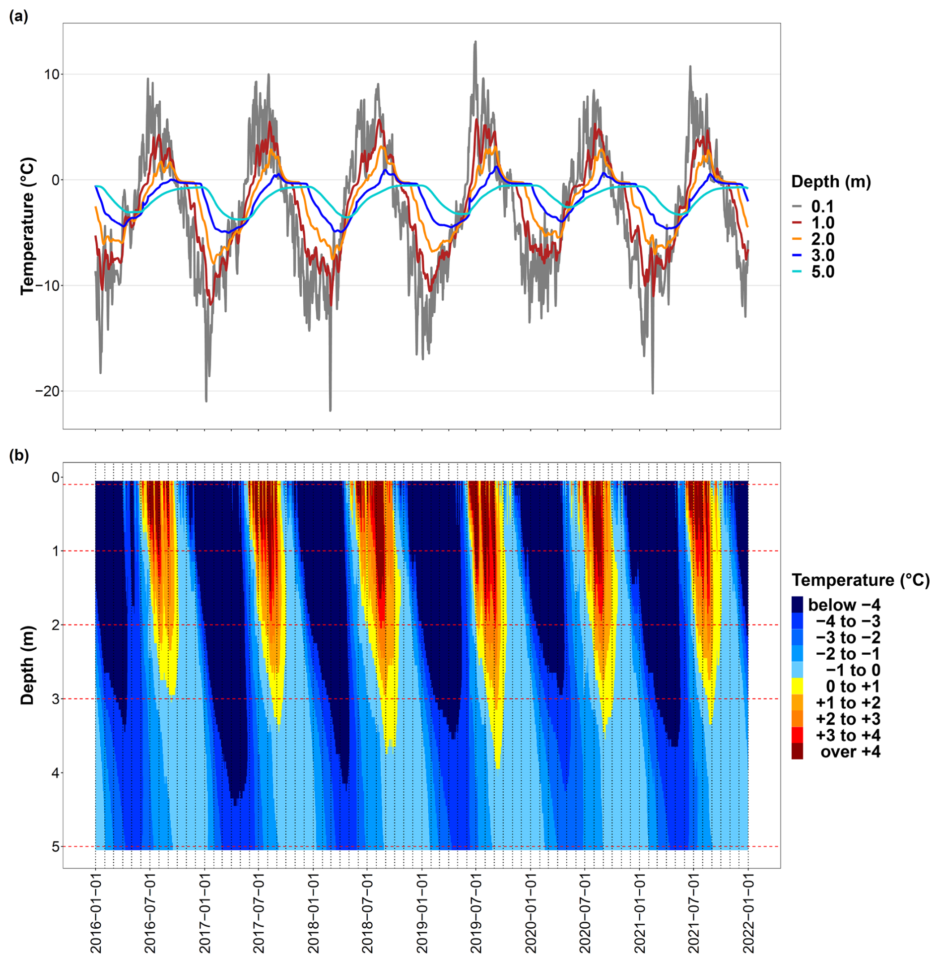
Figure 3 Temperature data and thawing process at the deep borehole (DB). (a) Measured ground temperature (daily mean values) at different depths. (b) Interpolated temperature data over depth and time (spline) as temperature classes. The red dashed cross lines refer to the depths at which temperature was measured (sensor depth).

Table 3 Characteristic values of the annual temperature wave at 0.1 m depth at the north-facing deep borehole (DB).

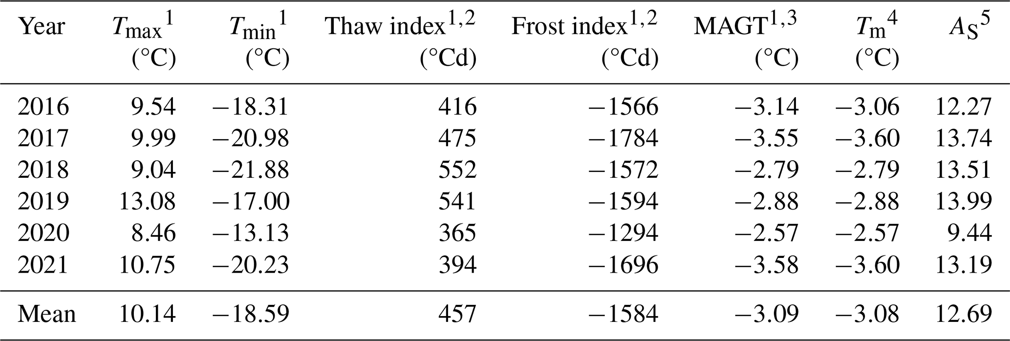
¹ Values calculated without curve smoothing. ² The thaw index is the temperature sum of all temperature values (daily averages) >0 °C. Accordingly, the frost index is the temperature sum of all temperature values (daily averages) <0 °C. ³ MAGT: mean annual ground temperature, calculated based on daily mean temperatures. ⁴ T_m is the mean annual ground temperature used to drive the analytical model and calculated based on a 5 d moving average of the daily mean temperature. ⁵ A_s is the amplitude at 0.1 m depth used to drive the analytical model calculated from half the distance between the extreme values (T_max and T_min) of the annual temperature wave after curve smoothing (5 d moving average).

Within the active layer, the mean annual ground temperature (MAGT) increased with depth (Fig. 4a). The mean thermal offset was 1.23 ± 0.23 °C between 0.1 and 3 m depth (within the active layer) and 1.42 ± 0.29 °C between 0.1 and 5 m depth. Accurate calculation of the damping depth from the phase shift (d_phase) was only possible for 2 years (2017 and 2018) and across three measurement depths, due to inharmonic temperature oscillations in the other years. As shown in Fig. 4b, the phase shift increased proportionally with depth, which is consistent with theory. In contrast, calculating the damping depth from the amplitude damping (d_amplitude) was possible for all years. Down to a depth of 3 m, the amplitude damping was rather homogeneous in depth (Fig. 4c). This indicates that thermal diffusivity was nearly constant down to that depth and that there were no significant depth-dependent differences (e.g., due to water saturation changes). It also indicates that amplitudes were exponentially more damped with increasing depth, as expected from theory. Between 3 and 5 m depth, the amplitudes were less damped due to a higher thermal diffusivity. Here, the thermal diffusivity α_amplitude calculated from amplitude damping was 0.89 ± 0.22 × 10⁻⁶ m² s⁻¹ on average over 6 years. For modeling the annual thaw process and ALT, the thermal diffusivity between 0.1 and 3 m (within the active layer) is more important.

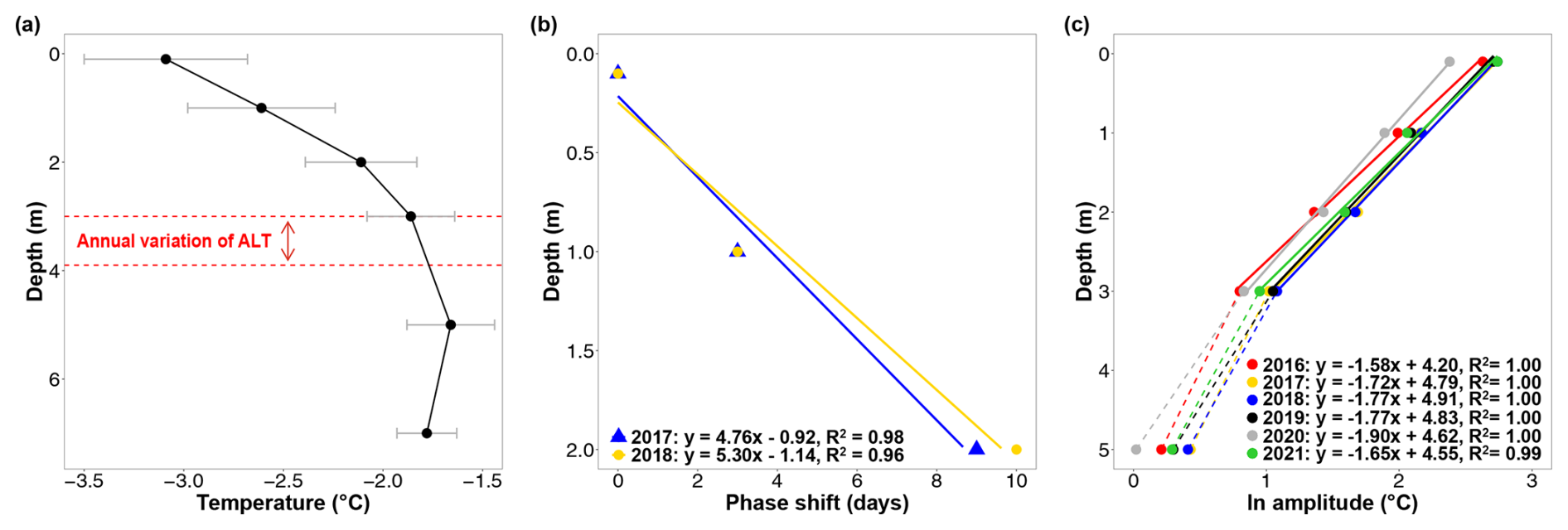
Figure 4 (a) Mean annual ground temperature (MAGT) at different depths from 2016 to 2021. Due to sensor failure, data from 2020 and 2021 are missing at a depth of 7 m. Error bars represent the standard deviation of the interannual variations, and the two red-dashed lines indicate the maximum and minimum variations of the active layer thickness (ALT). (b) Phase shift of the annual temperature wave with depth and the corresponding regression lines. Due to inharmonic oscillations, this could only be calculated over three depth levels and for only 2 years. (c) Damping of the annual temperature amplitude (natural logarithm (ln) of the temperature amplitude) with depth, along with the corresponding regression lines. Amplitude damping down to a depth of 3 m was highly consistent (R²≈1), which is critical in terms of magnitude for wave thermal propagation into the subsurface. The scattered lines show the amplitude damping between 3 and 5 m depth (not included for calculating regression lines), i.e., within the permafrost. The amplitude damping between active layer and permafrost was lower than in the profile above.

Table 4 summarizes the estimated damping depths and calculated thermal diffusivities of the active layer, where the values of d_phase were larger than those of d_amplitude. Two basic theoretical assumptions for the analytical solution of the heat equation (Eq. 4) warranted a critical assessment, which is why the thermal diffusivities calculated via Eq. (6) could only be regarded as approximations: first, the MAGT was only constant to a rough approximation due to the thermal offset with depth. Second, the investigated temperature waves do not describe harmonic oscillations. This could already be seen in Fig. 3a and was further confirmed by the fact that d_phase was 0.97 m larger than d_amplitude. The damping depth calibrated via the modeling process (d_calibrated) was 2.4 m and thus lay within the interval of d_phase and d_amplitude and relatively close to the mean value of d_phase and d_amplitude, which was 2.2 m.

Table 4 Damping depths from phase shift (d_phase) and amplitude damping (d_amplitude), and the corresponding calculated thermal diffusivities (α_phase, α_amplitude).

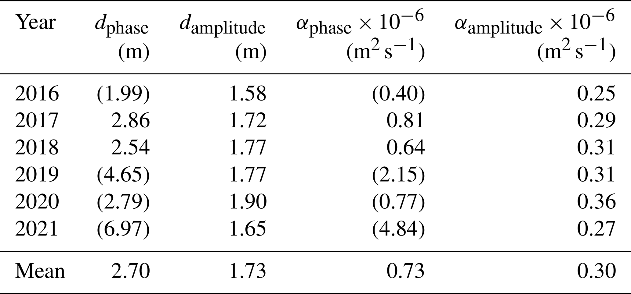
The values of d_phase without brackets were calculated between 0.1 and 2 m depth using linear regression over three depths (0.1, 1, 2 m). In contrast, the values of d_phase in parentheses were only calculated over two depths (1–2 m) without linear regression and were not included in the mean value calculation due to high uncertainty. The values of d_amplitude were calculated using linear regression over four depths (0.1, 1, 2, 3 m). To calculate the thermal diffusivity α, a period length (P) of 365 d was assumed.

4.2 Modeling active layer thickness at the deep borehole

The thawing process was successfully modeled based on daily values. During the validation period, the NSE was 0.79 (0.36 without model adjustment in the onset of the autumnal freezing period; see Sect. 3.2), exceeding the required threshold of >0.7 for successful modeling (Fig. 5a and b). The main modeling focus was the annual values of ALT. In 2016 (calibration period), the model showed the largest deviation from the measured value (Fig. 5a). In that year, the surface-penetrating amplitude was also damped the most (Fig. 4c) and α_amplitude was consequently the smallest (Table 4). For the remaining years, ALT could be modeled with satisfactory accuracy over the entire study period. In the validation period (three data pairs), the RMSE was 0.13 m, well below the required maximum threshold (<0.2 m), indicating successful modeling, and a close match between measured and modeled ALT values (Fig. 5c).

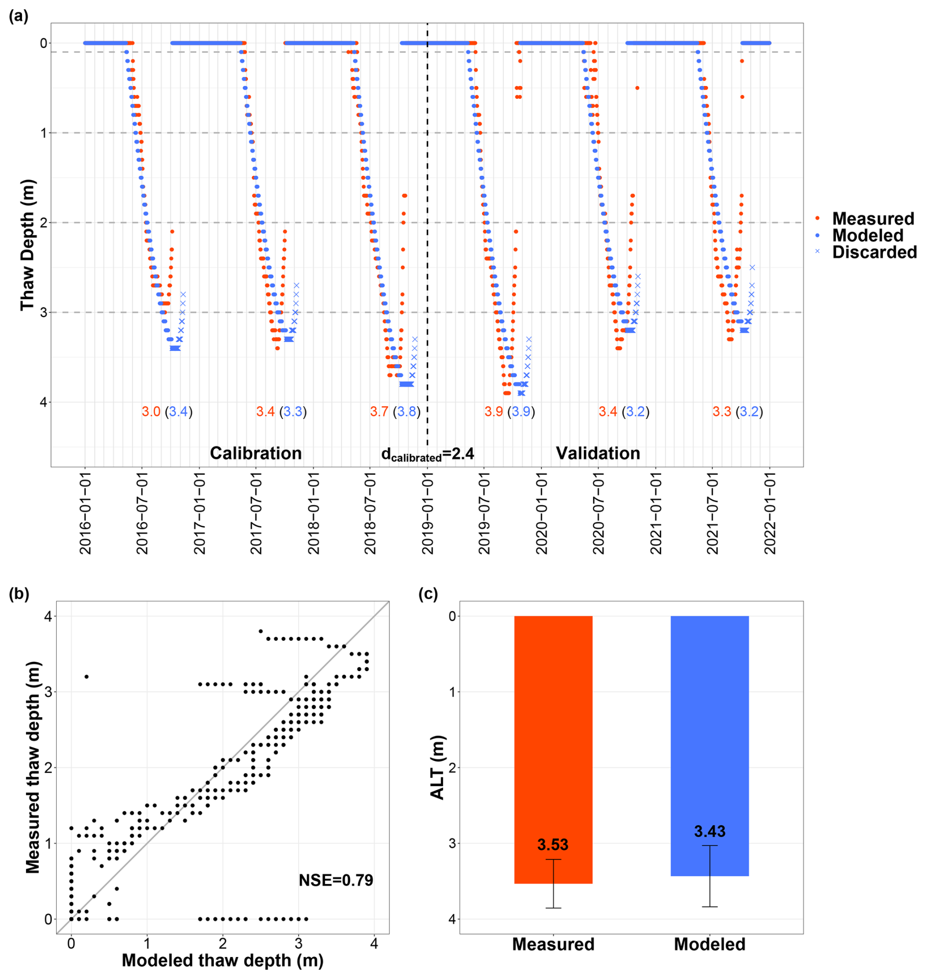
Figure 5 (a) Daily measured and modeled thaw depths at the deep borehole (DB). The calibrated damping depth (d_calibrated) expresses the thermal diffusivity for thermal wave propagation with depth. The onset of the autumnal frost process could not be represented well, so modeled values for the time after the annual thaw depth maximum were discarded and replaced by the value zero. The red (measured) and blue (modeled) numbers represent the annual values of the active layer thickness (ALT). The dashed horizontal lines indicate the depths at which temperature was measured (sensor depth). (b) Scatterplot of daily measured and modeled thaw depths for the validation period; gray line = line of equality; NSE = Nash–Sutcliffe efficiency coefficient. (c) Mean values of the measured and modeled ALT of the validation period; the error bars show the standard deviation.

4.3 Spatial and future projection of active layer thickness

Table 5 shows ALT values for the studied deep borehole (DB) and the four shallow boreholes (SBs). The west- (SB 1), east- (SB 3), and south-facing (SB 4) boreholes (Table 2) were the warmest (Appendix C). At SB 3, five out of seven modeled years showed a positive MAGT calculated with a sliding average for analytical modeling (T_m; see Sect. 3.2); no consecutive years with a negative T_m were found. This indicates that permafrost was not present there. Permafrost was present at SB 1 and SB 4, but 1 year with a positive T_m was also observed at each of the two sites. In contrast to SB 1 and SB 4, which had similarly high ALT values, the two north-facing boreholes (DB and SB 2) showed a much smaller ALT. In direct comparison, the ALT at SB 2 was 0.5 ± 0.2 smaller than at DB (average of 2016 to 2019).

Table 5 Measured (deep borehole = DB) and modeled (shallow borehole = SB) values of the annual maximum thaw depths in meters.

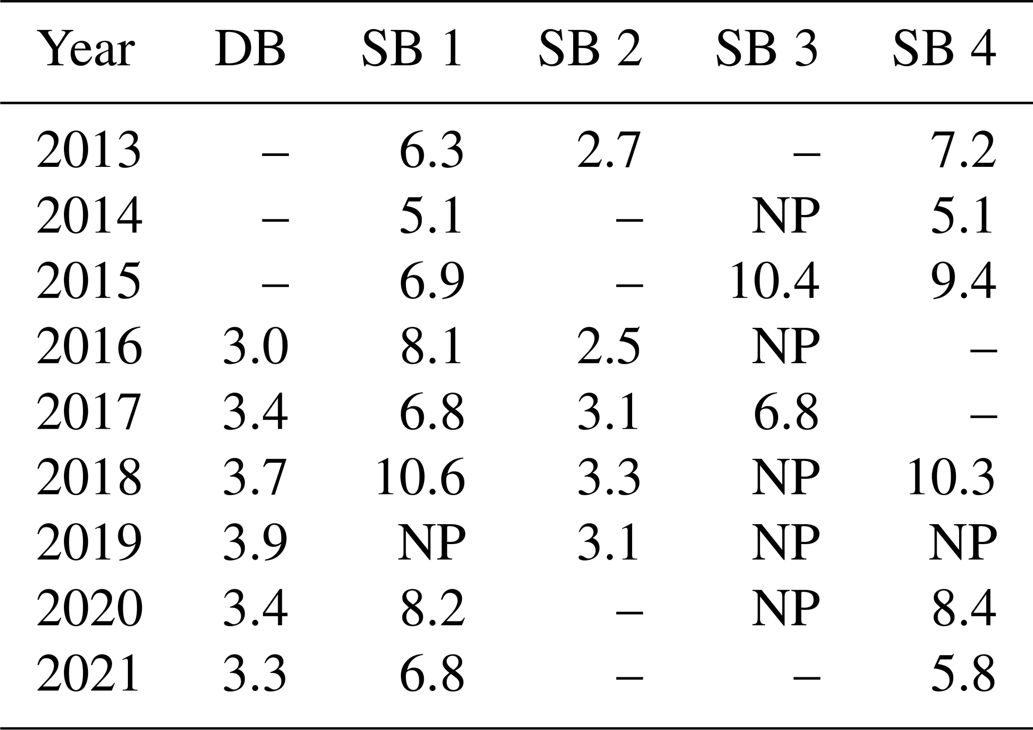
NP denotes no permafrost; (–) indicates data gaps due to measurement failures.

It has to be noted that the model results do not reflect potential lateral heat flow between SB sites. In reality, such heat flows would certainly occur between the closely grouped trio SB 2–4, which would significantly reduce the high ALT variability between the sites. Modeled ALT values therefore should be interpreted as idealized representations of their respective slope aspect not affected by three-dimensional (3D) topography effects.

Following SSP1-2.6, permafrost will no longer be present at SB 1, SB 3, and SB 4 by mid-century after an increase in T_m. Projections of the future ALT could only be made for the coldest north-exposed boreholes DB and SB 2 (Fig. 6). Towards mid-century, the model showed an increase in the ALT of 48 % under SSP1-2.6 and 76 % under SSP5-8.5. Towards the end of the century, permafrost at SB 2 can only be expected under scenario SSP1-2.6 with an ALT increase of 51 %. At the slightly warmer DB, the model showed a 62 % increase in the ALT under SSP1-2.6 and a 128 % increase under SSP5-8.5 toward mid-century. Toward the end of the century, permafrost at DB can only be expected under scenario SSP1-2.6 with a 69 % increase in the ALT.

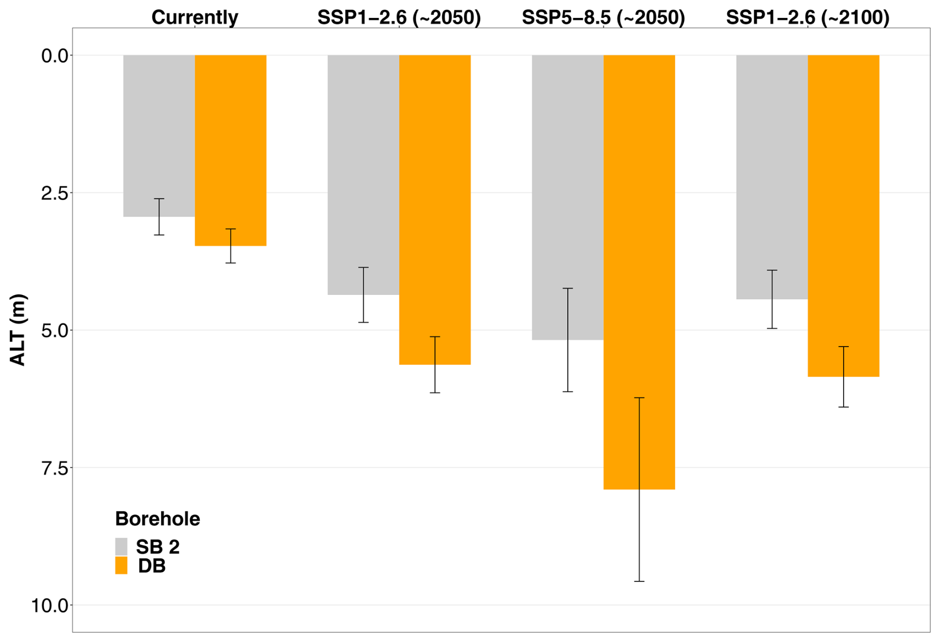
Figure 6 Projections of future active layer thickness (ALT) assuming scenarios SSP1-2.6 and SSP5-8.5 for mid-century, and regarding only SSP1-2.6 for the end of the century, at the deep borehole (DB) and shallow borehole 2 (SB 2). Towards the end of the century, permafrost can only be expected to occur in these two coldest, north-facing boreholes under scenario SSP1-2.6. The current ALT was calculated on the basis of all measured values during the study period, whereby the years included in the calculation were different in some cases (see Table 5). The colored bars show the mean values, the error bars the standard deviation.

5 Discussion

5.1 Ground temperatures at the deep borehole

Mean annual ground temperature (MAGT) rises with increasing depth within the active layer. This positive thermal offset of the MAGT with depth is surprising. An opposite (negative) thermal offset is a well-known phenomenon in polar regions (Burn and Smith, 1988; Romanovsky and Osterkamp, 1995; Smith and Riseborough, 2002) and was also already detected in mountain (bedrock) permafrost (Hasler et al., 2011), usually caused by a seasonal variation of the water saturation and its phase changes in the subsurface (Gruber and Haeberli, 2007). These variations cause the cooling front to usually penetrate the profile more deeply than the heating front, resulting in a negative thermal offset. However, Hasler et al. (2011) also observed a positive thermal offset within the active layer for one out of nine temperature observations in mountain (bedrock) permafrost.

At the deep borehole the positive thermal offset was likely caused by (i) convective heat flow due to significant subsurface meltwater flow during the thaw period, combined with (ii) an increase in thermal diffusivity due to increased water saturation with depth: at the onset of each thaw season (around June), we observed small, sharp temperature jumps at 2, 3, and 5 m depth, typically by a few tenths of a degree. These abrupt changes can only be attributed to fluid heat flow (convection) in joints and not by conduction-driven warming. This observation is consistent with optical scan data from the deep borehole, which demonstrates open, surface-parallel (∼45°) joints along the natural schistosity of the bedrock (calcareous mica schist) that form ideal pathways for subsurface lateral water flow. Recent geoelectrical and piezometric measurements from the Kitzsteinhorn confirm these assumptions and demonstrate the temporary presence of liquid subsurface water (Offer et al., 2025). In addition, the zero-curtain effect observed in the measured temperature waves, which is caused by release of latent heat during the phase change from water to ice (Outcalt et al., 1990), became more pronounced with increasing depth and was strongest at 3 m depth within the active layer. At the end of the thaw period, water saturation at depth was therefore increased.

Depth-dependent damping of annual amplitudes was remarkably homogeneous, and consequently no large changes are to be expected for vertical heat transport over the depth range studied. However, this refers to the damping of annual amplitudes and therefore does not necessarily exclude temporary water flow, which is likely to be responsible for the observed thermal offset. Within the permafrost body, i.e., below the active layer, amplitude damping was less pronounced. This is most likely related to the phase change of joint and pore water, since ice has a thermal diffusivity roughly five (James, 1968) to eight times (Oke, 1987; Garratt, 1994) higher than liquid water.

5.2 Modeling active layer thickness at the deep borehole

We successfully modeled ALT with an analytical solution of the heat transport equation based on near-surface temperature data (0.1 m depth). The accuracy of the modeled ALT was satisfactory. During the validation period (three data pairs, 2019–2021), the RMSE is 0.13 m, well below the required threshold (<0.2 m; see Sect. 3.2), indicating successful modeling. The largest deviation between measured and modeled ALT was observed for 2016 (calibration period), with a value of 0.4 m. In that year, the surface-penetrating temperature amplitudes were damped the most, and the calculated thermal diffusivity (α_amplitude) was the smallest during the study period. In line with that, the largest differences between the calibrated damping depth (d_calibrated) and the damping depth calculated from amplitude damping (d_amplitude) were also observed in 2016. No significant structural changes are expected in the bedrock of the calcareous mica schist over the study period. Therefore, it is reasonable that a lower joint and pore water content decreased thermal conductivity (Kim and Oh, 2019) and thus α_amplitude, and as a result caused the largest model deviations in that year. The thawing process was successfully represented based on daily values, with an NSE of 0.79, which is well above the required threshold (>0.7; see Sect. 3.2), further demonstrating the model's reliability. In contrast, the onset of autumnal active layer freezing was not well represented, likely due to the model's inability to account for altered thermal conductivity during phase changes.

While joint and pore water certainly had some influence (thermal offset and a zero-curtain effect within the active layer), the combined evidence from the (i) remarkable homogeneous damping of temperature amplitudes with depth (Fig. 4c), (ii) smooth temperature change over time and depth without abrupt jumps (apart from small temperature jumps at 2–5 m depth at the onset of each thaw season), and (iii) excellent model results from a model approach that is exclusively conduction-based, clearly indicates that conduction is the dominant heat transfer mechanism for local ALT formation. Laboratory tests of local calcareous mica schist core samples demonstrate an effective porosity of only 0.3 %–0.4 % (see Sect. 2 and Appendix D). Based on this low porosity we assume that the effect of latent heat transport is only marginal and has no significant effect on ALT formation, which thus supports the validity of excluding latent heat effects from our model.

For the application of the analytical solution of the heat transport equation, two basic assumptions must be considered critically: first, the MAGT was not constant with depth (z) or was constant only as a very rough approximation. Second, the annual temperature waves did not describe harmonic oscillations. Temporal variability of weather conditions is the main reason for the deviation of annual air and ground temperature oscillations from an ideal sinusoidal pattern (Rajeev and Kodikara, 2016). Nevertheless, the good calibration and validation possibilities at DB permitted a relatively robust estimation of the calibrated damping depth (d_calibrated). In ideal harmonic oscillations, the values of d_amplitude and the damping depth derived from phase shift (d_phase) are approximately equal. This was not the case in our study; however, d_calibrated (2.2 m) fell within the range of d_phase and d_amplitude and was relatively close to their mean value (2.4 m). This indicates a high plausibility that d_calibrated can physically describe the vertical conductive heat transport for modeling the thawing process.

5.3 Spatial and future projection

Following model development with data from the DB, we applied the model to the shallow boreholes and integrated IPCC climate scenarios for future ALT simulations. The chosen depth of 0.1 m, as a near-surface boundary condition, offers the advantage that temperature is undisturbed by turbulent heat flows on the ground surface – furthermore, this depth inherently accounts for the effect of any potential snow cover. Our modeling approach did not take into account topography-induced 3D effects on the ALT; instead, we considered the SBs as idealized representatives of their slope aspect, which are not affected by lateral subsurface heat flow from other sides of the summit pyramid. Due to the study area's uniform lithology, we furthermore assumed that thermal properties at the SBs did not significantly differ from the DB, and that d_calibrated can be transferred to the SBs.

In the study area, slope aspect is the dominant topographic factor influencing ALT due to small elevation differences between the investigated boreholes (∼200 vertical meters). As a result, the smallest ALT (2.5–3.9 m) was found at the two north-facing boreholes DB and SB 2, which are both characterized by clear permafrost conditions. Large ALT values between 5 and 10 m were found at SB 1 and SB 4. Under current climatic conditions no permafrost is indicated for SB 3; the subsurface, however, could still contain relict permafrost produced by cooler conditions in the past. Somewhat surprisingly, apart from 2019, the south-facing borehole SB 4 is slightly colder (Fig. C1, Table C1) and thus has a higher permafrost probability than the east-facing borehole SB 3. This is most likely related to differences in rock wall gradients and their impact on local, small-scale snow cover patterns. The south-facing borehole SB 4 is located in a moderately steep rock wall section that hosts a small, thick snowpack during winter, spring, and early summer. While this insulation efficiently prevents the propagation of cold winter temperatures into the subsurface (warming effect), it also leads to a significant delay of seasonal warming (cooling effect) as compared to the east-facing SB 3, which is exposed to direct sunlight the entire year and, due to its steep gradient (∼80°), absorbs significant amounts of solar radiation even at low sun angles (winter season).

While slope aspect has been demonstrated here as a key factor for ALT evolution, this example illustrates that the topo-climatic disposition (slope aspect, slope gradient, elevation, topographic shading) can potentially be altered by local snow cover effects. The discussed influence of slope aspect is therefore straightforward only under the assumption of a uniform snow cover regime. Here, it is important to add that small-scale (∼ a few m²) snow cover effects have a pronounced influence on ALT model results, due to their dependence on temperature measurements carried out just 0.1 m below the rock surface. Consequently, our approach overestimates ALT sensitivity to small-scale snow cover variations, as the real seasonal ALT values result from thermal forcing over larger areas. This case emphasizes the significance of selecting representative sites for SB measurement and demonstrates the challenge of reconciling processes across different spatial scales.

ALT projection under scenario SSP5-8.5 suggests that, by mid-century, mountain permafrost will only be present at the north-facing boreholes, with a significant increase in ALT. Toward the end of the century, however, permafrost is expected to disappear entirely, even at these two coldest boreholes, under this scenario. However, uncertainties in the future projection exist, particularly related to future snow cover patterns and the insulating properties of the snow cover, which leads to seasonal decoupling of atmospheric and ground surface temperatures. Despite these uncertainties, a key conclusion transferable from this projection to other permafrost regions is that a larger initial ALT (DB: 2.9 compared to SB 2: 3.5) will also lead to a larger increase in ALT for the same temperature rise (regarding SSP5-8.5 for mid-century, SB 2: 56 %, DB: 128 %). This shows that in warm permafrost, even small changes in temperature cause large increases in ALT, which has significant implications for rock and slope stability. Study results from the Western Alps point to increased rockfall activity along the lower permafrost boundary, i.e., in regions with (already) large ALT. Rockfall documentation from Switzerland demonstrates a late-summer peak in rockfall activity in regions with warm permafrost around 3000 m a.s.l. (Kenner and Phillips, 2017) and analyses of a century-long inventory of slope failures from the central European Alps (France, Italy, Switzerland) indicate increased mass wasting in low-lying permafrost regions (Fischer et al., 2012). As global warming is expected to continue or even accelerate, this trend will most likely be reinforced over the next decades. Warming-induced upward migration of the lower permafrost boundary may result in a slight altitudinal shift of rockfall activity, while active layer thickening will most likely activate deeper failure planes and cause larger rockfall volumes – and will require significantly deeper foundations for constructions on permafrost.

5.4 Potential applications of analytical ALT modeling

Despite limitations in accurately modeling ground temperature on a daily scale due to the neglection of latent heat, convection, and altered thermal conductivities during phase changes, our approach demonstrates for the first time that ALT in steep bedrock environments can be effectively modeled using a simple, time- and cost-efficient method. The chosen analytical solution to the heat conduction equation adequately captures the local thermoregime and overcomes the constraints of numerical models in terms of accuracy when relying on a limited number of field measurement points, computational costs for simulation runs, and reliable parameter optimization and identification. Unlike numerical approaches, our method allows for straightforward and fast predictions of ALT under varying boundary conditions (idealized model forcing) without requiring expertise in numerical modeling. Estimating ALT based on near-surface bedrock temperature, combined with analytical modeling, thus offers a practical and powerful tool that could be integrated into expert systems for bedrock permafrost regions. As the study area does not exhibit highly specific site conditions that would distinguish it from other steep bedrock environments, our findings are likely applicable to other active layers in predominantly conduction-driven systems (bedrock).

Due to the widespread availability of near-surface bedrock temperature data, our ALT model approach can be readily applied at numerous other high-alpine sites with adequate temperature datasets and similar boundary conditions.

Low computational demands, along with the absence of complex and highly site-specific calibrations, furthermore hold the theoretical potential for large-scale application, e.g., at the scale level of an entire mountain range. This would, in a first step, require the development of a near-surface bedrock temperature model, for example following an empirical–statistical approach based on key topographic parameters verified by local bedrock temperature data. Using such a model, large-scale estimations of ALT could be performed, akin to previous studies that employed similar approaches to model the probability of permafrost occurrence (Schrott et al., 2012). While an ALT model of this type would involve considerable inaccuracies related to the modification of the ALT through snow cover dynamics and 3D topography effects, it could serve as a valuable tool for quantitative permafrost and natural hazard assessment in complex, high-alpine terrain.

6 Conclusions

The active layer thickness (ALT) in mountain permafrost, an increasingly critical factor for natural hazard management, is particularly responsive to climate change. This is especially true for steep permafrost rock walls, which are highly sensitive to air temperature fluctuations due to their typically thin snow cover and low subsurface ice content (limited pore volume), which reduces the delaying effect of latent heat processes. In the present study, we used borehole temperature data from the summit region of the Kitzsteinhorn (central Eastern Alps, Austria) to model ALT. We draw the following conclusions.

• To model ALT, we analytically solved the conductive heat transport equation through sinusoidal thermal waves that propagate into the subsurface. A 6 year dataset from a 30 m deep bedrock borehole was used for model calibration and validation. So far, simulations of the ALT (bedrock permafrost) have been based on numerical models; the present study reports the first analytical solution to the heat transport equation to model ALT in permafrost rock walls (borehole scale) and offers a concise, process-based understanding of how (modified) input parameters impact the studied system.

• Measured and modeled ALT values were highly consistent: during the validation period (2019–2021), modeled and measured ALT at the deep borehole (DB) differed by only 0.1 ± 0.1 m, with a root mean square error (RMSE) of 0.13 m, well below the required maximum threshold (<0.2 m), indicating successful modeling. Additionally, the thawing process was accurately represented based on daily values, with a Nash–Sutcliffe efficiency coefficient (NSE) of 0.79, which is well above the required threshold (>0.7), further demonstrating the model's reliability.

• We used the developed thermal model to simulate ALT at four shallow boreholes (SBs, 0.1 m deep) located in close proximity and found that the modeled ALT ranged between 2.5 m (SB 2) and 10.6 m (SB 1) in the observation period (2013–2021). Due to small differences in altitude (∼200 m) within the study area, slope aspect had the strongest impact on the ALT; however, this effect can potentially be modified by snow cover effects.

• Under the more moderate SSP1-2.6 scenario, by mid-century ALT is expected to increase by 48 % at SB 2 and by 62 % at DB, while permafrost will no longer exist at SB 1, SB 3, and SB 4.

• The impact of a temperature increase on ALT is more pronounced when the initial ALT is higher. This suggests that in warm permafrost, even small rises in temperature can lead to substantial increases in ALT, which has significant implications for rock and slope stability.

• In contrast to permafrost soils, which have higher porosity and water content, latent heat appears to play a secondary role in the annual ALT evolution of bedrock permafrost with very low pore volumes. This condition makes the use of this relatively simple modeling approach possible.

• With its mathematical simplicity, lack of complex parameterization, and the widespread availability of near-surface temperature data, our model is directly applicable to a wide range of other steep bedrock sites. By incorporating topography-based estimates of near-surface ground temperatures, ALT could be modeled at larger spatial scales in the future. Integrating latent heat exchange and altered thermal conductivities through phase changes and the effects of advective heat transport in joint and pore water could be useful improvements of the presented analytical modeling approach, especially for higher porous media and wet conditions where latent heat flow may play a more prominent role.

Appendix A: Measured and interpolated temperature data at the deep borehole

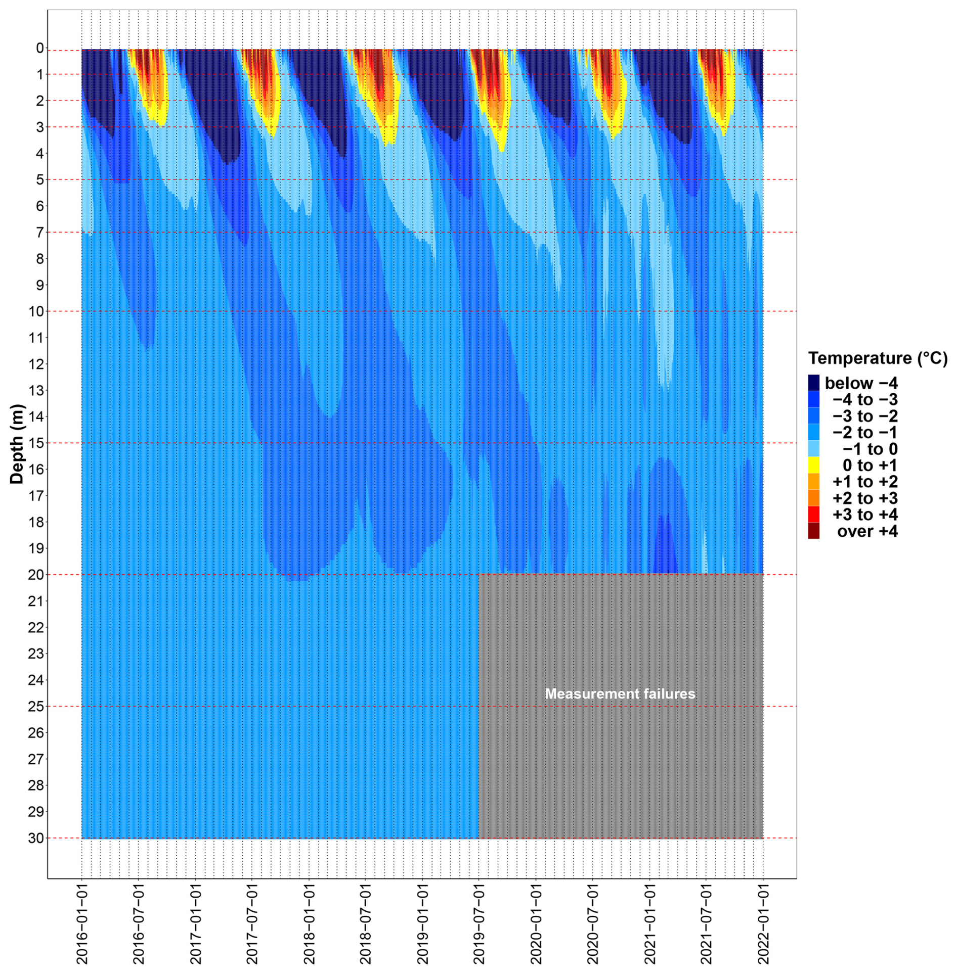
Figure A1 Interpolated temperature data over depth and time (spline) as temperature classes. The red dashed cross lines refer to the depths at which temperature was measured (sensor depth). In the gray filled area, the values could not be displayed accurately due to measurement gaps. The temperature sensor at 7 m depth has also failed since 14 June 2020, which is why the interpolation values between 5 and 10 m may be less precise from then on.

Appendix B: Yearly trumpet diagrams for the deep borehole

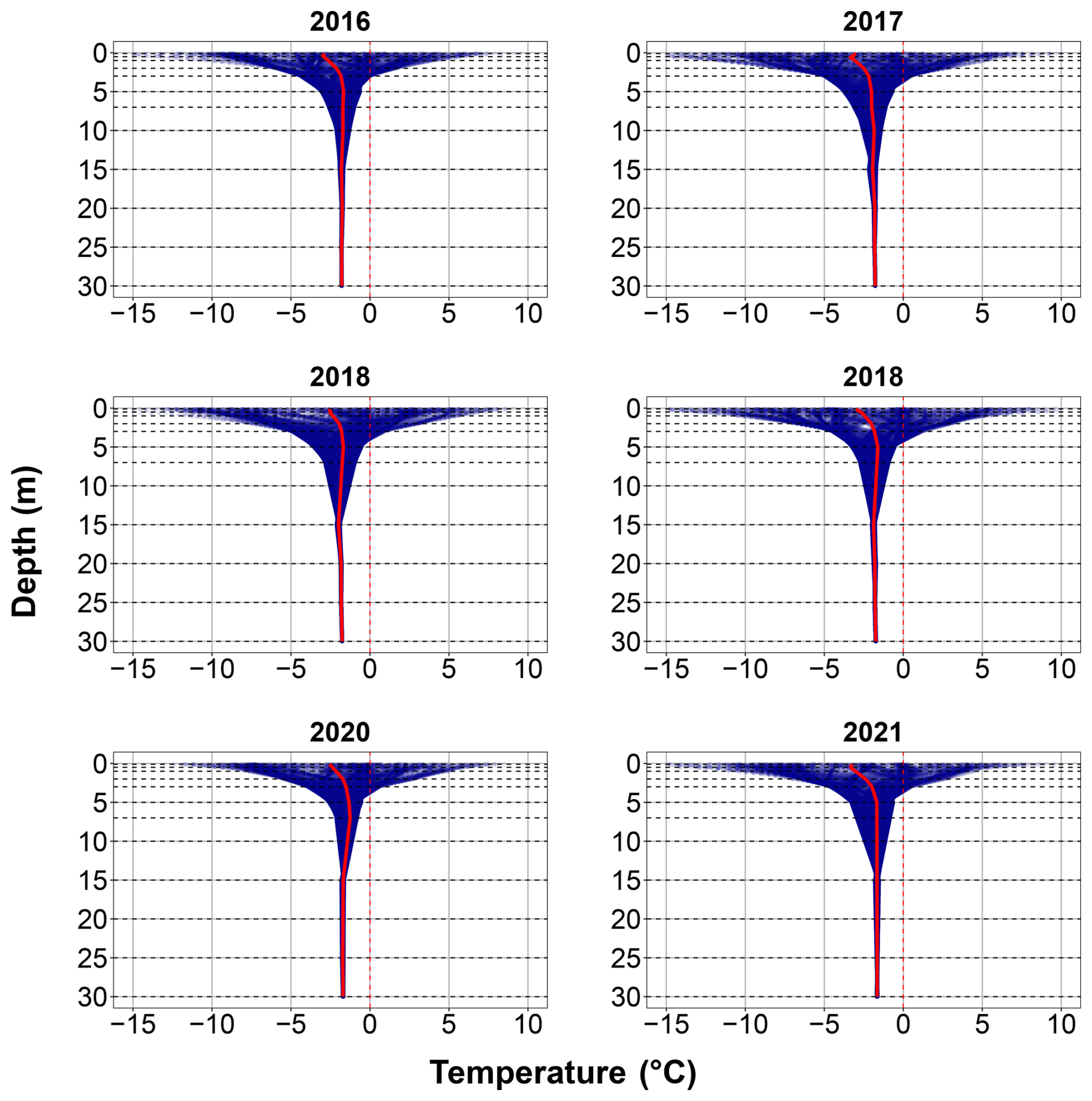
Figure B1 Yearly trumpet diagrams (depth vs. temperature) for the deep borehole (DB) based on daily mean temperature (2016–2021). Sensor depths are indicated by dotted horizontal lines. Temperature values between sensor depths is derived from linear interpolation. Solid, red line represents annual mean temperature.

Appendix C: Temperature data at the four shallow boreholes

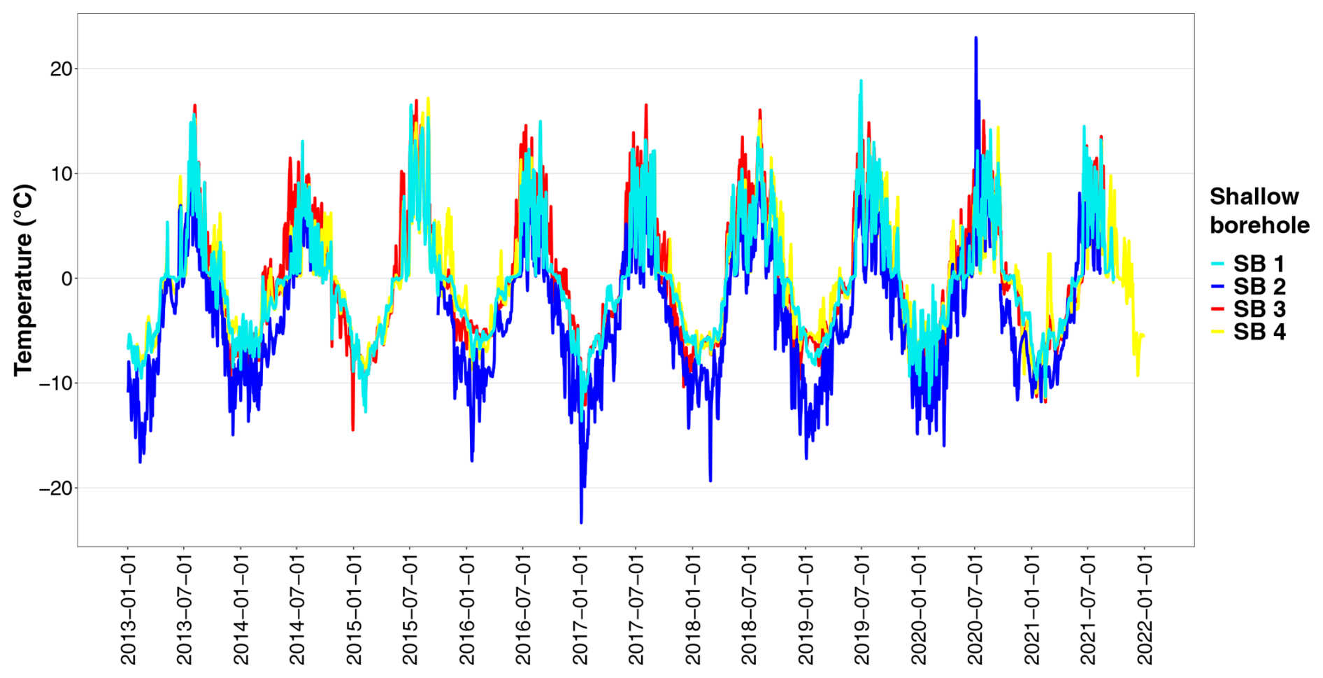
Figure C1 Measured ground temperature (daily mean values) at the shallow boreholes (SBs) investigated. In some cases there were large gaps in the data, in which case the temperature lines are shown as interrupted.

Table C1 Values for the analytical modeling, calculated from the temperature wave at a depth of 0.1 m in °C.

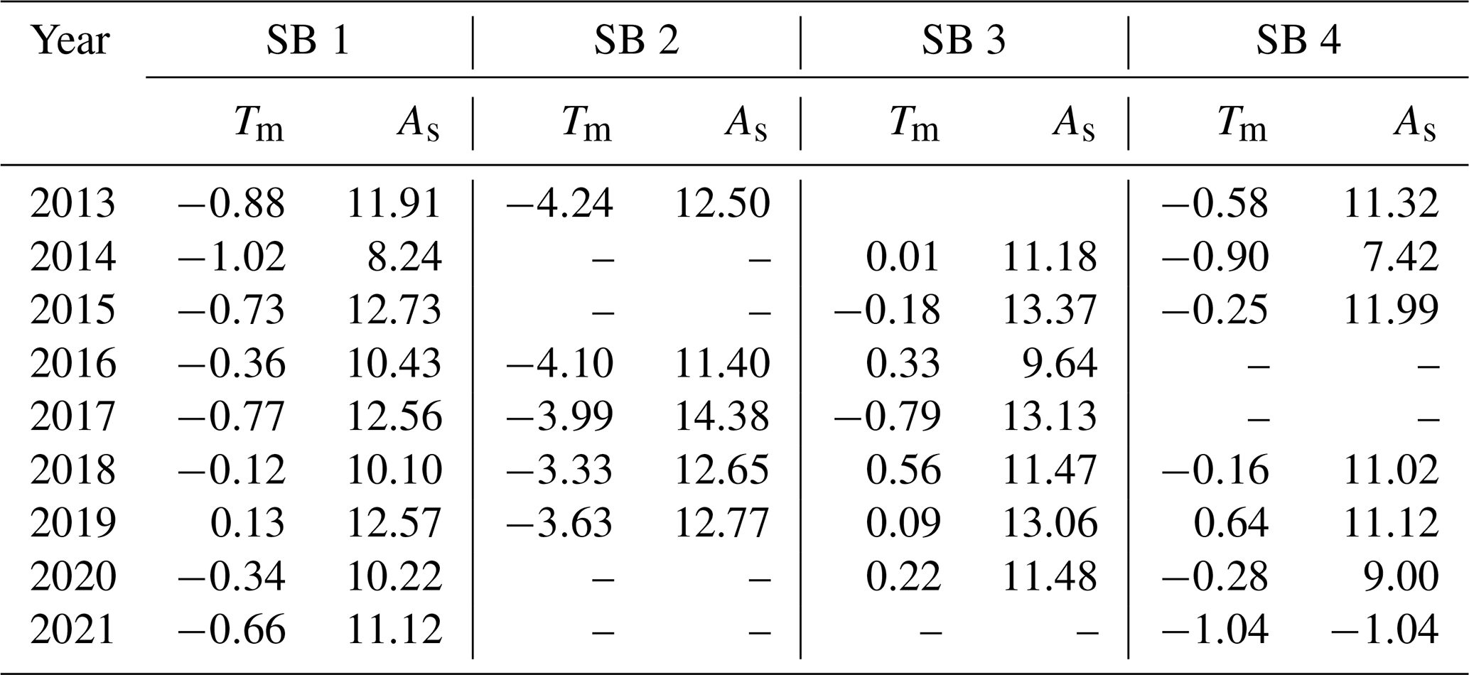
The temperature wave (daily averaged temperatures) was smoothed with a moving average of 5 d. T_m is the mean annual ground temperature and A_s is the temperature amplitude calculated from half the distance between the extreme values (T_max and T_min) of the annual temperature wave; a dash (–) indicates data gaps due to measurement failures. Both model parameters served as surface boundary conditions for analytical modeling.

Appendix D: Determination of porosity values on local core samples

Table D1 Characteristics and physical properties of calcareous mica schist core samples.

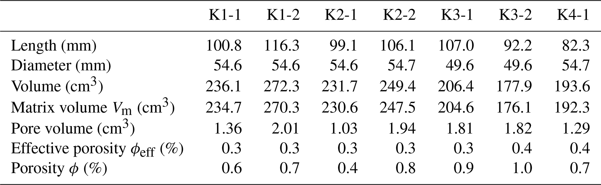
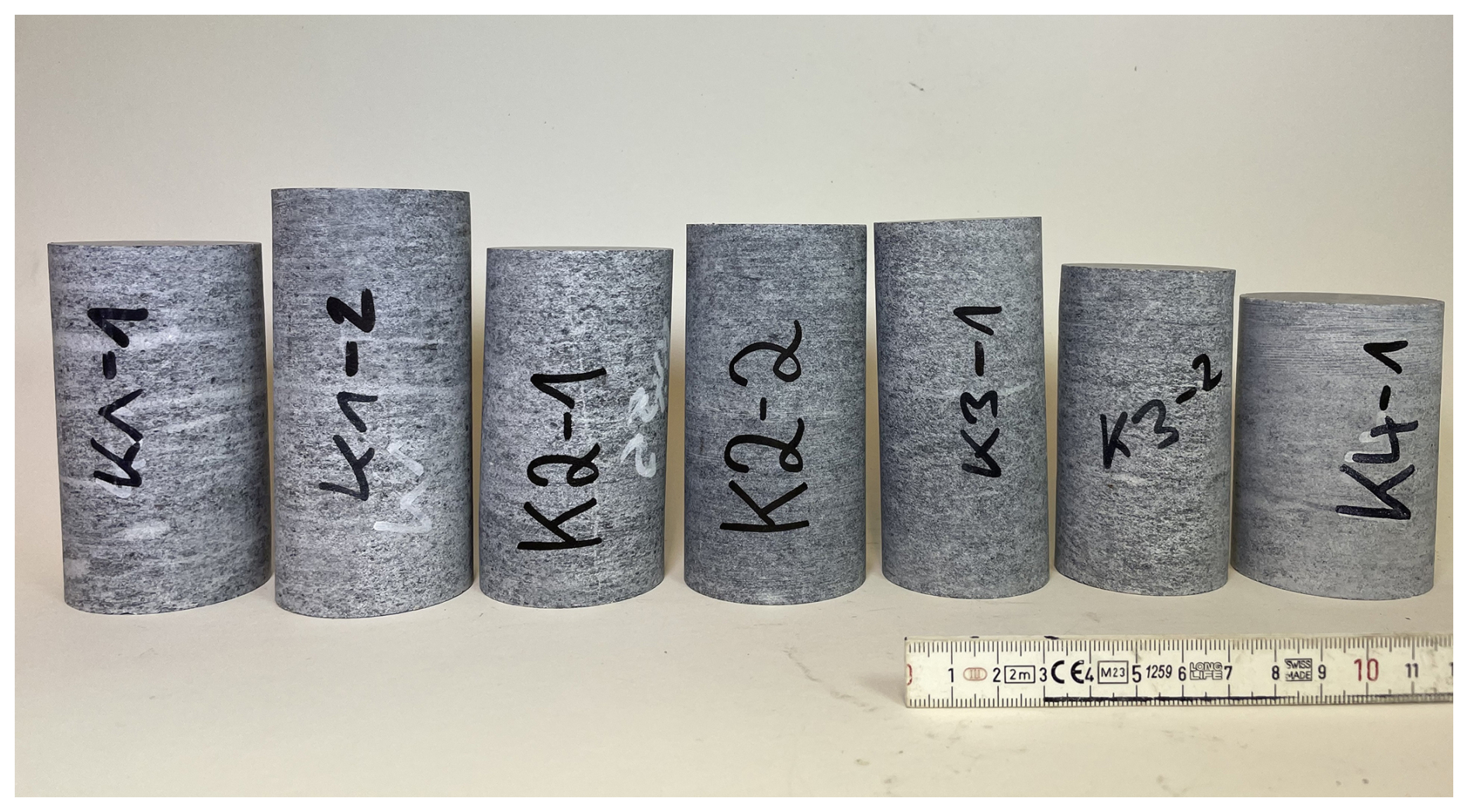
Figure D1 Photograph of seven calcareous mica schist cores used for porosity tests. (Photo taken by Maike Offer.)