Translating deposition ages into erosion rates: inverse landscape evolution modelling and uncertainty analysis

Soil erosion is a significant threat to agricultural food production. Determination of erosion rates is essential for quantifying land degradation, but it is challenging to determine temporally dynamic erosion rates over long time scales. Optically Stimulated Luminescence (OSL) dating can provide temporally-resolved deposition rates by determining the last moment of daylight exposure of buried colluvial deposits. However, these deposition rates may differ substantially from the actual hillslope erosion rates.

In this study, hillslope erosion rates were derived from OSL-based deposition ages through inverse modelling with soil-landscape evolution model ChronoLorica. This model incorporates geochronological tracers into simulations of soil mixing and redistribution. The model was applied to a closed catchment in north-eastern Germany, which has experienced tillage erosion over the last 5000 years. Previously reconstructed pre-erosion topography and land-use history, with known uncertainties, allowed for an uncertainty analysis to quantify the impacts of various sources of uncertainty on the model output.

The inverse modelling provided local tillage parameters for different land-use phases that aligned well with a global compilation from comparable studies. The simulated erosion and deposition rates, which increased by two order of magnitude over time, correspond well with independent age controls at both the catchment and point scales. On average, deposition rates were 1.5 times higher than the erosion rates, with recent increases up to five times, indicating that deposition rates cannot be used as direct proxies for erosion rates. The uncertainty analysis showed that the initial topography was the dominant source of variance in the model output, followed by land-use history and model parameters. Reconstruction of these initial and boundary conditions with their uncertainty is essential for representing uncertainty in model output and avoiding overconfidence in the model. This study demonstrates the suitability of ChronoLorica for upscaling experimental geochronological data to better understand landscape evolution in agricultural settings.

1 Introduction

Soil erosion is one of the main threats to agricultural land and food provision, because it reduces agricultural productivity by loss of fertile soil (Rhodes, 2014). Soil erosion is not only a problem of recent times. Already in the prehistoric, the first land use activities, such as deforestation and manual hoeing, triggered soil loss by removing the protective vegetative cover and loosening up the soil (Dreibrodt et al., 2010; Vanwalleghem et al., 2017). With developments in agricultural practices and an increase in food demand, agricultural activity and consequently soil erosion increased over time. In current intensively managed landscapes, where land use is heavily mechanized, averaged rates of soil loss can exceed 15 t ha⁻¹ a⁻¹ (Nearing et al., 2017).

Historical anthropogenic erosion rates were significantly lower compared to modern-day rates, yet their cumulative impact over centuries of agricultural use may have contributed substantially to overall land degradation. It is inherently challenging to resolve temporally dynamic erosion rates over long time scales, especially in systems where land use and erosion rates have changed over time (Loba et al., 2022). Geochronometers such as radionuclides can provide erosion rates that are averaged over timescales that depend on their half-lives, such as cosmogenic nuclides (Granger and Schaller, 2014), or on the moment of introduction in the landscape, such as fallout radionuclides (Mabit et al., 2008; Peñuela et al., 2023). Other geochronometers, such as radiocarbon dating or optically stimulated luminescence (OSL) dating do have the ability to provide temporally resolved rates by dating layers from different depths. However, these techniques provide deposition rates instead of erosion rates, as they rely on deposited or buried material. These deposition rates can act as proxies for erosion rates, but will also be affected by other factors, such as the ratio between erosional and depositional area, the sedimentological connectivity of the hillslope and the capacity to store sediments in depositional locations. Deposition rates can therefore deviate substantially from the actual erosion rates, which could lead to erroneous evaluation of land degradation.

In this work, deposition ages determined with OSL dating will be translated into erosion rates using inverse landscape evolution modelling. OSL dating measures the built-up luminescent signal in soil minerals (often quartz or feldspar), that accumulates due to ionizing radiation in the subsurface and incoming cosmic radiation. The luminescence signal resets when the soil particle is exposed to daylight and is therefore a proxy for the duration of burial (Murray and Roberts, 1997). Advances in numerical soil-landscape evolution models enable the tracing of geochronometers such as OSL particles and radionuclides with simulated mixing and transport processes over decadal to millennial timescale (e.g. Furbish et al., 2018; Van der Meij et al., 2023). Through inverse modelling, soil mixing and erosion rates could be derived from OSL ages. For transient landscapes, such as agricultural landscapes, such a modelling exercise requires detailed information on the major erosion processes that occur in the landscape, the initial shape of the terrain and land use history during the evolution of the landscape (Tucker and Hancock, 2010; Perron and Fagherazzi, 2012; Finke et al., 2015). These initial and boundary conditions come with uncertainty, especially when they have to be reconstructed beyond timespans where observations are available. This uncertainty should be quantified and incorporated in simulations of soil and landscape evolution to better convey our confidence in the model results (Perron and Fagherazzi, 2012; Minasny et al., 2015). Through comparison with independent data and age controls, the validity of the calibrated parameters and their uncertainty can be tested (Temme et al., 2017).

The objectives of this paper are to test (1) whether OSL-based deposition ages can be translated into erosion rates through inverse soil-landscape evolution modelling, (2) how these rates are affected by uncertainties from initial conditions, boundary conditions and calibrated parameters, and (3) how the reconstructed rates compare to rates derived from other geochronological methods. The simulations were performed with soil-landscape evolution model ChronoLorica, which couples geochronological tracers to simulations of soil redistribution (Van der Meij et al., 2023).

2 Study area

2.1 Site description

The study area is the agricultural landscape laboratory CarboZALF-D (Fig. 1, Sommer et al., 2016). This site is located in the young morainic landscape in north-eastern Germany, which formed after the last glacial retreat in the Weichselian around 19 ka ago (Lüthgens et al., 2011). The parent material is illitic, calcareous glacial till. Annual rainfall is around 480 mm and annual mean temperature is 8.7 °C. The first agricultural practices started around ∼ 5 ka ago, with intensification in the last 1000 years (Kappler et al., 2018; Van der Meij et al., 2019; Öttl et al., 2024). The area remained under agricultural use until it was converted into a landscape laboratory in 2010. Now, only certain sections are still cultivated.

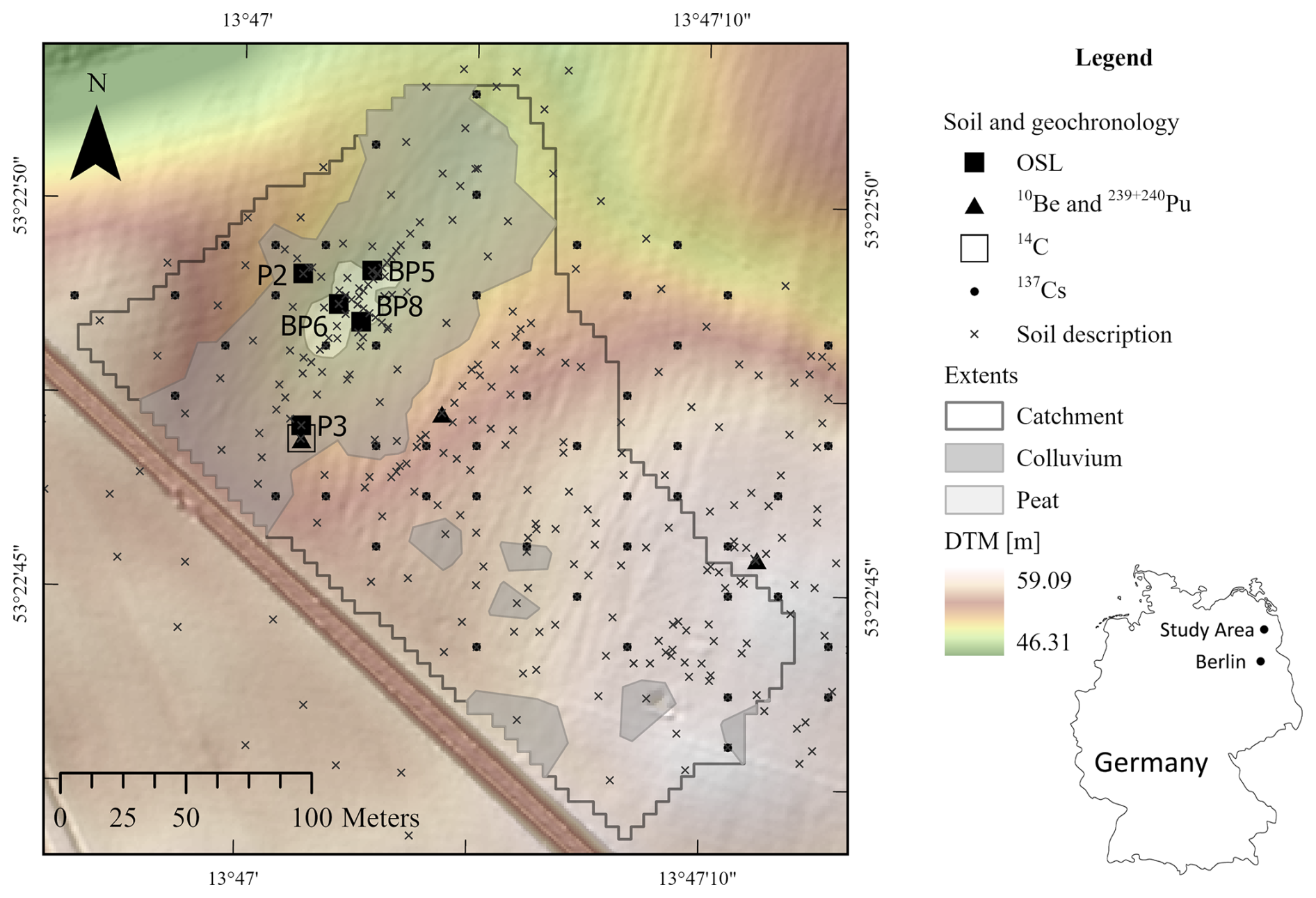
Figure 1 Map of the study area CarboZALF-D, showing the locations where the geochronological samples and soil descriptions were taken. The grey shaded areas indicate where colluvium and peat are currently present.

CarboZALF-D is a closed kettle hole catchment, meaning that almost all eroded sediments are stored in the central depression, providing unique opportunities for studying erosion processes and landscape reconstruction. This includes a reconstruction of the paleo-topography before anthropogenic erosion using truncation of soil profiles (Van der Meij et al., 2017), determination of deposition rates and patterns using optically stimulated luminescence (Van der Meij et al., 2019), determination of short-term and long-term erosion rates using ^239+240Pu and meteoric and in-situ ¹⁰Be (Calitri et al., 2019), and determination of recent erosion rates using ¹³⁷Cs (Aldana Jague et al., 2016). Altogether, this resulted in a large geochronological dataset covering different spatial and temporal scales (Fig. 1).

2.2 Landscape evolution at CarboZALF-D

CarboZALF-D underwent a complex landscape evolution. Van der Meij et al. (2019) identified five different periods of plough use and land-use intensity (Table 1) and dated 32 OSL samples from five different locations in the colluvium (Figs. 1 and 2). Based on the datings and land-use history, they could identify two distinct layers of colluvium (Fig. 2). The first layer of old colluvium, with ages from 5 ka up to 300 a, was deposited at the fringes of the colluvium, but did not reach into the central kettle hole. This centre area was probably too wet for agricultural practices, as identified by the peaty layer that is still present under the colluvium. Following drainage at the start of the 19th century to increase agricultural acreage, the central depression became accessible for agricultural practices. Continued erosion in the catchment, including re-erosion of the old colluvium, led to the deposition of a younger layer of colluvium in the central depression, that also covered the older colluvium at the fringes (Fig. 2). With modernization of agricultural tools and increased tractive power, recent erosion rates far exceed the (pre-)historical erosion rates (Sommer et al., 2008; Van der Meij et al., 2019). Overall, the hillslopes experienced an average erosion of 30 cm and the colluvial layers are on average 51 cm thick (Van der Meij et al., 2017). Most erosion occurred where the slope gradients increased around the central depression. The upper parts of the slope experienced less erosion. Deposition mainly occurred in the central depression, but there are also small colluvial patches located on the hillslopes. The reconstructed elevation changes are provided in Fig. 5a.

Table 1 Overview of reconstructed land management history at CarboZALF-D. Periods of different plough uses with corresponding mixing depths and their uncertainties are indicated. Modified from Van der Meij et al. (2019).

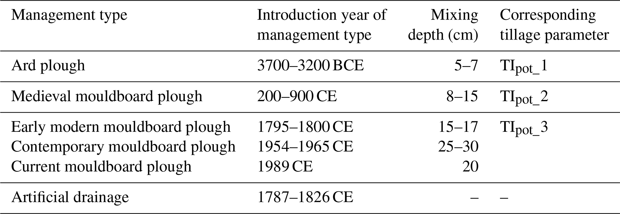
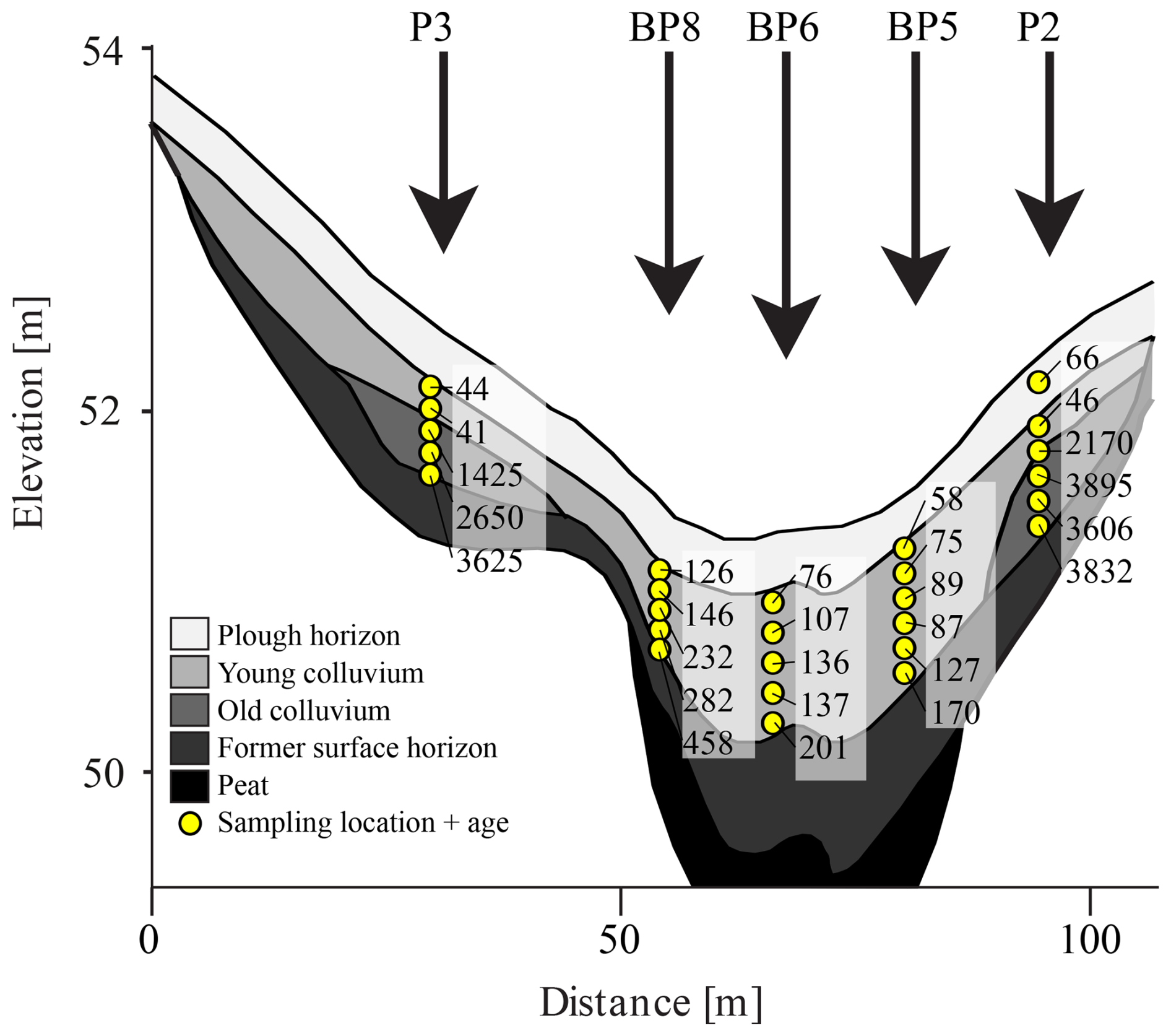
Figure 2 Positions of the OSL sampling locations projected on a SE–NW transect through the colluvial infilling of the depression. The indicated ages, corresponding to the modes of the measured age distributions, were used for the inverse modelling in this study.

The CarboZALF-D catchment was split by a railroad constructed around 1900 CE. The southwestern part of the catchment is relatively flat and most soil profiles are still intact (Van der Meij et al., 2017). Therefore, the assumption in this paper is that that part didn't contribute substantially to the build-up of the colluvium in the central depression. It was therefore left out of the analysis.

2.3 The erosion processes

In the young morainic landscape of north-eastern Germany, tillage is currently the dominant erosion process and played a substantial role in the past as well (Aldana Jague et al., 2016; Van der Meij et al., 2019; Wilken et al., 2020; Öttl et al., 2024). This is best expressed in the erosion and deposition patterns, with most intensive erosion on convex hillslopes and deposition in concave positions (De Alba et al., 2004), which are observed in current agricultural landscapes and in comparable long-term (> 240 a) forested landscapes (Van der Meij et al., 2017; Calitri et al., 2020, 2021). These findings indicate that diffusive soil transport, caused by tillage erosion, has been the dominant erosion process in the study area. There are no visible traces of water erosion in the sediments, probably due to reworking of the sediments after deposition by tillage. Therefore, and to facilitate the modelling exercise, tillage is considered the sole erosion process in this study.

3 Methods

3.1 ChronoLorica

3.1.1 Model architecture

Soil-landscape evolution model ChronoLorica was used for simulating the landscape evolution (Van der Meij and Temme, 2022; Van der Meij et al., 2023). ChronoLorica is based on soil-landscape evolution model Lorica (Temme and Vanwalleghem, 2016), with the addition of a geochronological module. This module couples the soil and landscape forming processes to the redistribution of different geochronometers, in this case particle ages that are analogous to OSL ages. The landscape surface is represented by a raster-based elevation model. Below each raster cell there is a pre-defined number of soil layers. Inside each layer, the model keeps track of five texture classes (gravel, sand, silt, clay, fine clay). Changes in the mass of the soil constituents due to additions or removals is converted into a change in layer thickness and consequently elevation of the surface through the bulk density. The original Lorica model uses a pedotransfer function from Tranter et al. (2007) to calculate bulk density. This function predicts bulk densities of 1570 ± 40 kg m⁻³ for the parent material of CarboZALF-D, which is a systematic underestimation of measured bulk densities of 1720 ± 110 kg m⁻³ (Van der Meij et al., 2017). Therefore, a constant bulk density of 1720 kg m⁻³ was applied in this study. A more detailed description of the model architecture can be found in Temme and Vanwalleghem (2016) and Van der Meij et al. (2023).

The model results a three-dimensional representation of the soil landscape at different timesteps. This representation includes information on geochronometers at different depths, which facilitates comparison between simulated and measured depth functions of luminescence ages. This is not possible with most other landscape evolution models that only consider two-dimensional landscape surfaces without depth information.

3.1.2 Process descriptions

In ChronoLorica, tillage is simulated as a two-part process. The first part addresses the soil mixing. Over the range of the plough depth pd [m], soil layers are completely homogenized. This includes the mineral soil, organic components, stocks of radionuclides and particles with OSL ages.

The second part addresses lateral soil translocation by tillage. Tillage erosion and deposition follows a linear diffusion-type equation (Eq. 1, Govers et al., 1994). The transport of tilled material to a lower-lying neighbouring cell (TI_local, [m]) is a function of the potential tillage parameter TI_pot [–], local slope Λ_local [m m⁻¹] and the plough depth pd. TI_pot is distributed over all lower-lying neighbouring cells J, proportional to their slopes Λ_j.

$$\begin{array}{}\text{(1)}& {\mathrm{TI}}_{\mathrm{local}}={\mathrm{TI}}_{\mathrm{pot}}{\displaystyle \frac{{\mathrm{\Lambda }}_{\mathrm{local}}}{{\sum }_{j=\mathrm{1}}^J{\mathrm{\Lambda }}_j}}\times {\mathrm{\Lambda }}_{\mathrm{local}}\times \mathrm{pd}\end{array}$$

This formulation was used instead of the conventional diffusion Equation from Govers et al. (1994), because it explicitly considers the effect of plough depth on tillage redistribution. In Govers et al. (1994), this is included in the tillage transport coefficient k_til. Both equations are equivalent and can be transformed into each other through a bulk density and plough depth value. The model works with an annual timestep. After every tillage operation, the elevation model is updated with the additions and removals of soil materials. This also affects the slope gradients, which will be different in each calculation step.

ChronoLorica's particle age module keeps track of the location of a finite number of OSL particles throughout the simulations. The fate of the OSL particles is coupled to the sand fraction in the model, which is the fraction that is commonly selected for OSL dating. The age of the OSL particles increases with one year for every simulation year. The age of particles present in the surficial bleaching layer is reset to 0 every simulation year. Because the model works with a finite number of particles, a stochastic approach is used to determine whether an OSL particle is transported from a layer together with the bulk sediment. The uncertainty of this stochastic approach is constrained by simulating a large number of particles (∼ 150) per layer. The probability that a particle is transported by vertical or lateral redistribution processes (P_transport) is equal to the mass of redistributed sand [kg] divided by the total mass of sand in the source layer [kg] (Eq. 2).

$$\begin{array}{}\text{(2)}& P_{\mathrm{transport}}={\displaystyle \frac{\text{sand redistributed}}{\text{total sand present}}}\end{array}$$

3.1.3 Parametrization

The parent material of the soils was based on average parent material properties from CarboZALF-D soils (53 % sand, 34 % silt, 13 % clay, Van der Meij et al., 2017). The initial topography was derived from reconstructions based on soil profile truncations and colluvial additions to the current landscape (reconstruction 2c in Van der Meij et al., 2017). The initial soil profiles were 2 m deep, consisting of 40 layers of 5 cm. The amount of OSL particles was set to ∼ 150 grains per layer and the bleaching depth was set to 5 mm, which was based on model-based estimates (Furbish et al., 2018) and is in line with light penetration depths in rocks (0–15 mm, Meyer et al., 2018). Simulations were 5000 years with an annual timestep, through which plough depth and tillage intensity changed based on values in Table 1 and the calibrated tillage intensities (Sect. 3.2). To mimic the two-stage landscape evolution at CarboZALF-D, the central kettle hole, with the size of the current peat extent, was only included in the last ∼ 200 years, following the artificial drainage. Model output was provided every 100 years during most of the simulations and every 10 years after the artificial drainage.

3.2 Inverse modelling

The unknown parameter in the tillage equation (Eq. 1) is the potential tillage parameter TI_pot. This parameter was calibrated using the OSL dates from Van der Meij et al. (2019) through inverse modelling. Samples taken from the soil buried below the colluvium were excluded, leaving 27 OSL samples from five locations (Fig. 2). To account for changes in TI_pot in time, the periods of different management types were aggregated to three periods with each their own potential (but unknown) tillage rate TI_pot (Table 1). For each period, the average introduction year and plough depth were used in the inverse modelling. The first period is the ard plough period, from the start of the simulations (3000 BCE) until 550 CE, with seven OSL dates covering this timeframe. The second period is the Medieval mouldboard plough, lasting until 1800 CE. There are no OSL dates that fall in this period, probably because sediments from this period located on the fringes of the depression have been re-eroded when the central depression was reclaimed. It was still possible to calibrate a TI_pot for this period based on the total amount of sediments that was required for filling the central depression without eroding the fringes beyond where the OSL dates from period 1 were located. The final period lasted until the end of the simulations and represents the use of the modern mouldboard plough. For this period 20 OSL dates were available.

Due to the intensive mixing during erosion, transport and deposition, the OSL-age distributions show a clear mode that corresponds to the depositional event (Van der Meij et al., 2019). Therefore, the model was calibrated on the modal ages of the age distributions. For each OSL sample, the equivalent layer at the same location and same depth in the simulated soil landscape was identified and the mode of its simulated age distribution was derived. For samples for which there was no equivalent layer, for example due to too thinly simulated colluvium, a dummy age of two times the simulation time was used to ensure that such an error was penalized heavily. The three TI_pots were calibrated by minimizing the mean absolute error (MAE) between the modes of the measured and simulated age distributions.

3.3 Uncertainty analysis

There are several sources of uncertainty in this inverse modelling exercise, stemming from model set-up, model input and calibration and model evaluation (Perron and Fagherazzi, 2012; Temme et al., 2017; Skinner et al., 2018). It is uncommon in landscape evolution studies to address all these sources of uncertainty, as there is often limited or no information to quantify their uncertainty. The CarboZALF-D area provides a unique setting for assessing the effects of uncertain initial and boundary conditions and parameter sets on model output, as the initial and boundary conditions are reconstructed and their uncertainties are well-known, the landscape evolution is complex but only subject to one main process and there is independent data for verifying the calculated erosion and deposition rates.

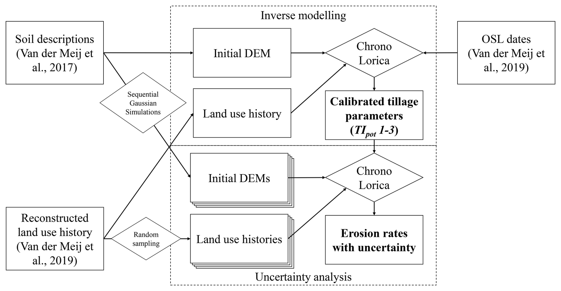
Figure 3 Workflow for the inverse modelling and uncertainty analysis in this study. Rectangles indicate data sources or results, while diamonds indicate methods and calculation steps.

In this study, I performed an uncertainty analysis to quantify the contributions of uncertainty from initial conditions, boundary conditions and the calibrated parameters on the model outputs (Fig. 3). The effect of other sources of uncertainty on the model outputs are discussed in Sect. 5.

For the reconstructed initial topography, 10 realizations of interpolated soil and colluvium thickness (Van der Meij et al., 2017) were made using Sequential Gaussian Simulation with the gstat package version 2.1-1 (Pebesma and Gräler, 2023), which randomly samples unique initial landscapes from within the interpolation uncertainty. For the boundary conditions, 10 land use histories with corresponding plough depths were randomly sampled from the values in Table 1, assuming uniform distributions for each range of values. For the model parameters, the 10 parameter sets for TI_{pot_}2 and TI_{pot_}3 that resulted the lowest calibration errors were selected. Variation in TI_{pot_}1 was not considered, as this parameter showed a clear optimal value, while the other parameters showed similar results for different parameter sets. The combination of the different initial topographies, land use histories and parameter sets produced 1000 unique model runs, which were used to quantify the sources of uncertainty and to present the mean and error ranges of rates of landscape change.

An ANOVA (analysis of variance) was conducted to quantify the contribution of the different sources of uncertainty to the variance in total erosion and total deposition. The analysis considered three groups of parameters, representing the initial conditions, boundary conditions and the parameter sets. These groups were used as independent variables in a linear model, with the total erosion or total deposition as dependent variable. The Sum of Squares of the ANOVA was then used to calculate the relative contributions of each group to the total variance. Assumptions of normality and homoscedasticity for the linear model and the ANOVA were tested with residual plots and QQ plots and were met.

3.4 Model evaluation

The simulated topographical changes and erosion and deposition rates from ChronoLorica were evaluated with different geochronological and erosion datasets. The simulated spatial patterns of erosion and deposition in the calibrated model run were compared with reconstructed elevation changes from Van der Meij et al. (2017). The simulated erosion and deposition rates resulting from the uncertainty analysis were compared with rates derived from OSL, ¹⁰Be, ¹³⁷Cs, ^239+240Pu and ¹⁴C data (Aldana Jague et al., 2016; Calitri et al., 2019; Van der Meij et al., 2019). The comparison of these rates was performed on a catchment scale and on a point scale for specific sampling locations.

4 Results

4.1 Model calibration

Figure 4a–e show the measured and calibrated age-depth profiles for all sampling locations for the model run with the lowest mean absolute error (MAE). The calibrated depth profiles follow the measured profiles, although some profiles are overall younger than simulated (P3, BP5), whereas other profiles are overall older than simulated (BP8). The mean absolute error (MAE) is highest for P2 and P3, where ages from the old colluvium were present (250 and 399 a). For the profiles from the central colluvium (BP5-8), the MAE ranges from 7–75 a. There is a good overall fit between the simulated and calibrated ages, with a MAE of 160 a and an R² of 0.96 (Fig. 4f). For the fringe positions P2 and P3, the simulated colluvium thickness is 6 to 14 cm shallower than observed, while the profiles in the central depression generally have a thicker simulated colluvium than observed (0, 7 and 17 cm).

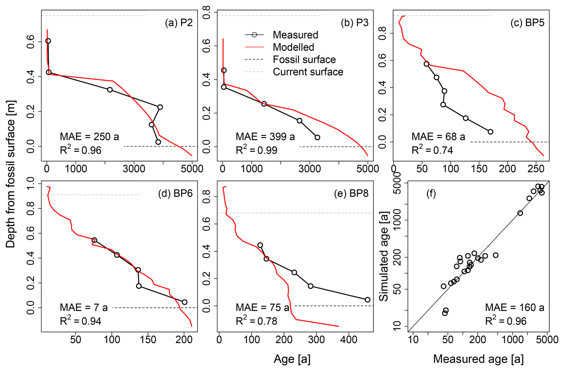
Figure 4 (a–e) Depth plots showing the modes of the measured and simulated ages of the calibration run with the lowest error for the different sampled profiles. The horizontal dashed lines indicate the observed levels of the fossil surface below the colluvium and the current soil surface. Mean absolute error (MAE) and R² are reported for all profiles. (f) Scatter plot of measured versus simulated ages. Note the logarithmic axes.

Since OSL particle tracing operates as a stochastic process, the distribution and ages of particles will be different between runs. To assess the impact of this on the calibration, a simulation was performed multiple times using the same parameter set. This resulted in a relative error of 0.2 % in the calibration error and had no discernible effect on the overall calibration outcomes.

Table 2 Results of the calibration of the tillage parameters for the different land-use periods. The spread in the parameters shows the calibration results from the 10 best runs, which were subsequently used in the uncertainty analysis. The corresponding k_til parameters were calculated using the ploughing depths from Table 1 and the bulk density of 1720 kg m⁻³. The last column shows median and 95 % confidence intervals of the reference values for tillage transport coefficient k_til compiled by Öttl et al. (2024), for similar plough types.

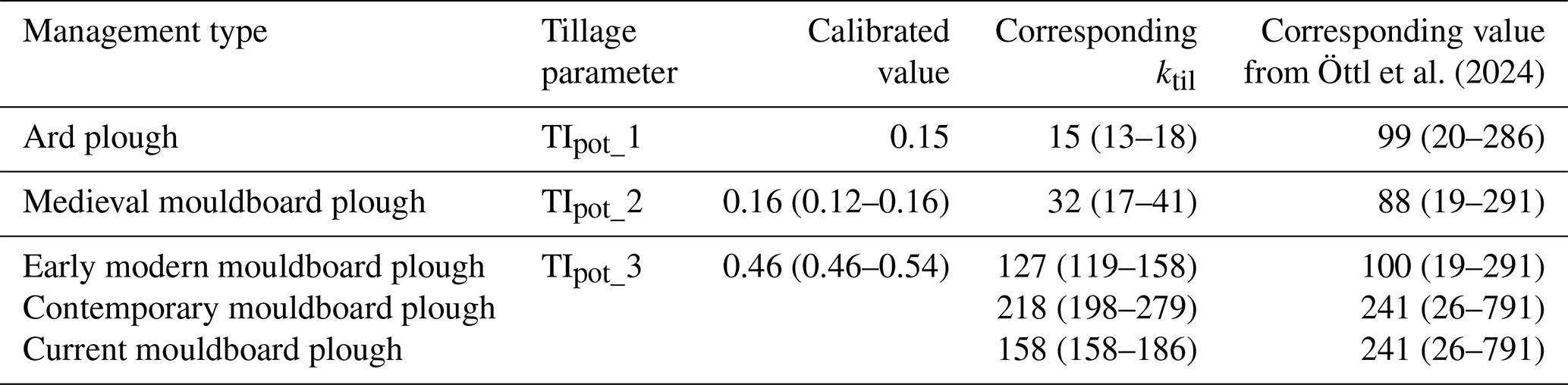
Table 2 shows the calibrated values for the tillage parameters for the different land-use periods. The parameters show an increase through time, with 0.15 for the period of the ard plough, 0.16 for the period of the Medieval mouldboard plough and 0.46 for the period of the modern mouldboard plough. The spread reported for TI_{pot_}2 and TI_{pot_}3 indicates the values for the 10 model runs with the lowest errors. The errors of these runs were within 2 % of the lowest error. The error ranges are not normally distributed and the model run with the lowest error has values at the edges of these ranges. Parameter sets from the 10 best runs were used in the subsequent uncertainty analysis. The corresponding k_til values were calculated for each land-use period, using the bulk density of 1720 kg m⁻³ and the reconstructed plough depths (Table 1). These values also show an increase through time, with a small decrease in the most recent period. The intensity in the ard plough period and Medieval mouldboard period were 7 % and 15 % of the contemporary tillage intensity.

Compared to the compilation of k_til values from Öttl et al. (2024), the k_tilcalibrated for the ard plough falls below the reported values (Table 2). The other plough types fall within the reported intervals, where the Medieval mouldboard plough is at the lower end and the more recent mouldboard ploughs have values comparable to the reported medians.

4.2 Reconstructed and simulated elevation changes

The simulated elevation changes with ChronoLorica resemble the reconstructed elevation changes by Van der Meij et al. (2017) (Fig. 5a, b). The extent of the central colluvium is smaller in the simulations, while the size of depositional areas on the hillslope is slightly larger. The differences between the reconstructed and simulated elevation changes (Fig. 5c) indicate that the elevation changes due to erosion were more similar between the reconstruction and simulation, compared to the elevation changes by deposition. Overall, absolute differences in simulated and reconstructed elevation were 16 cm on average, with greater overall erosion and deposition in the reconstructed map compared to simulated map.

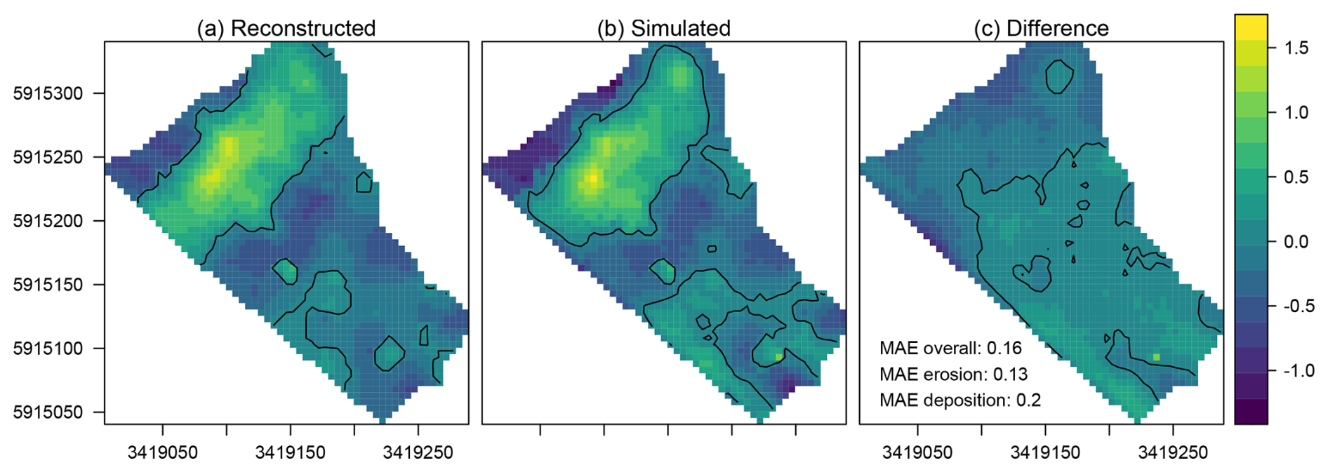
Figure 5 Elevation changes derived from (a) reconstructions with field data (Van der Meij et al., 2017), (b) the calibrated simulations and (c) the difference between both maps (simulated minus reconstructed). Contour lines indicate elevation differences of 0 m.

4.3 Erosion and deposition rates

The simulated erosion and deposition rates vary by two orders of magnitude over the simulation time, following changes in the land-use history (Fig. 6a). The catchment-averaged erosion and deposition rates (solid lines) start with 0.4 mm a⁻¹ at the start of the simulations and drop an order of magnitude during the period of ard ploughing. The transition to the period of the Medieval mouldboard plough shows an increase of the rates to 0.08 mm a⁻¹. The rates in the period of the modern mouldboard plough are again much higher, in the order of 4 mm a⁻¹. The 95th percentiles of elevation change (dashed lines) show the same trend, but with rates of 3–4 times higher than the catchment-averaged rates. The rates start around a millimetre per year at the start of the simulations after which they drop to 0.1 mm a⁻¹. During the Medieval mouldboard plough period, the rates are around 0.2 mm a⁻¹ and increase 1 to 5 mm a⁻¹ in the Modern mouldboard plough period, with a peak of up to 1 cm a⁻¹ just after the transition to this final phase.

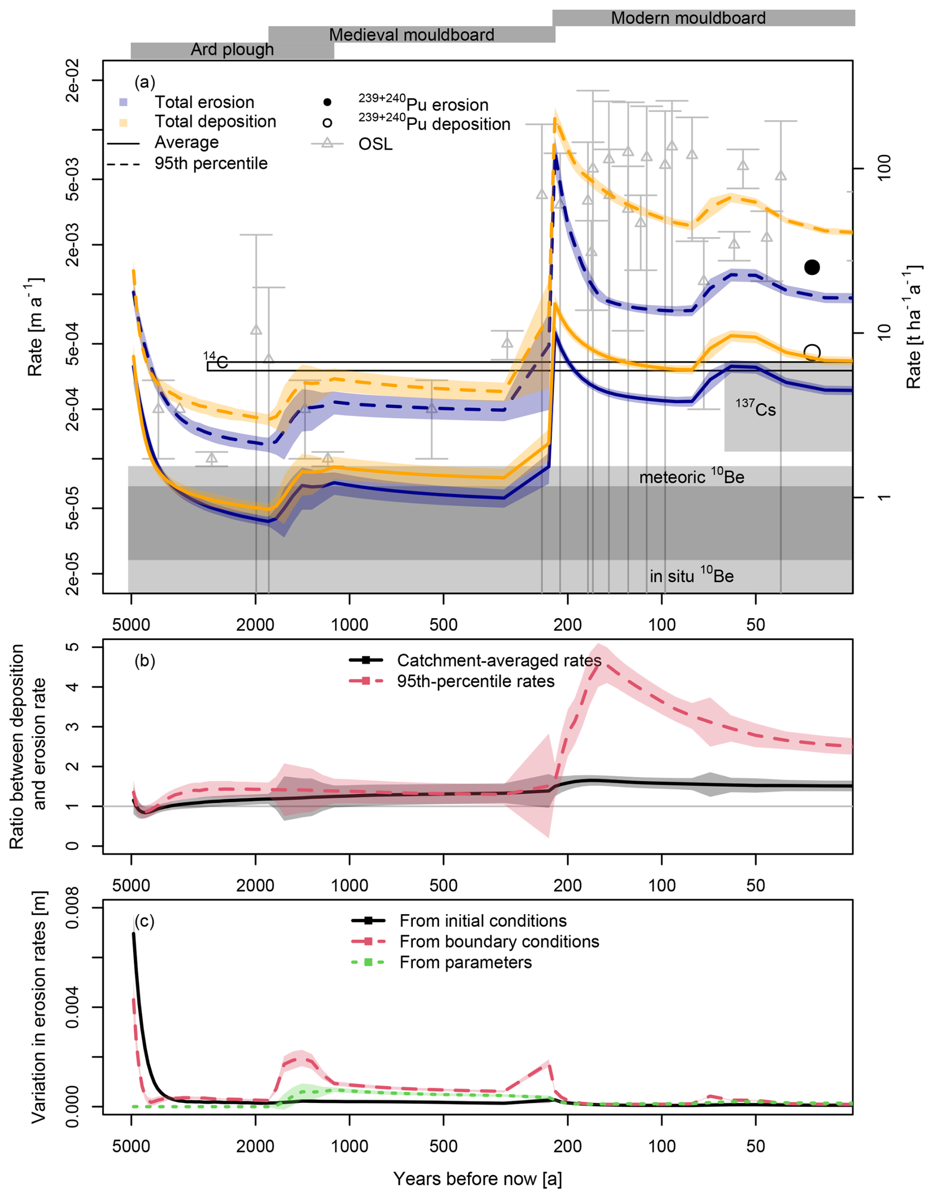
Figure 6 (a) Compilation of simulated and measured erosion and deposition rates. Simulated rates are provided in the blue (erosion) and orange (deposition) uncertainty bands and lines, for the catchment-averaged rates (solid lines) and the 95th percentile of erosion and deposition rates to represent severe erosion and deposition locations (dashed lines). Experimental data is provided with either rectangles representing their representative periods and corresponding rates with uncertainty, or as point information. Closed rectangles and symbols represent erosion rates, while open rectangles and symbols represent deposition rates. All provided uncertainties are 1σ intervals, except for ¹³⁷Cs (80 % interval). (b) Ratio between deposition and erosion rates, for catchment-averaged and 95th-percentile rates, provided with mean and 1σ uncertainty. Numbers larger than 1 indicate higher deposition rates. (c) Time-resolved variation in erosion rates coming from uncertainties in initial conditions, boundary conditions and calibrated parameters, expressed as the standard deviation in catchment-averaged erosion rates. Note the logarithmic x axis and y axis in panel (a).

With the exception of the first ∼ 1000 years, deposition rates are 1–1.5 times higher than erosion rates (Fig. 6b). In the last ∼ 220 years, following the drainage and cultivation of the central depression, catchment-averaged deposition rates are about 2 times as high as the erosion rates, while the 95th-percentile deposition rates can increase up to five times as high as the erosion rates.

On the catchment scale, rates derived from the experimental geochronological data follow the same trends as the simulated rates (Fig. 6a). In-situ and meteoric ¹⁰Be, representing averaged erosion over the entire period that this landscape exists, show rates in and below the lower regions of the simulation. The recent catchment-averaged rate derived with ¹³⁷Cs is in the same order of magnitude as simulated catchment-averaged erosion and deposition rates from that same period. Rates derived with OSL and ^239+240Pu lean towards the higher end of the simulated rates. The 95th-percentile deposition rate curve follows the same temporal trend as the OSL-derived rates, and falls largely inside the uncertainty of these rates.

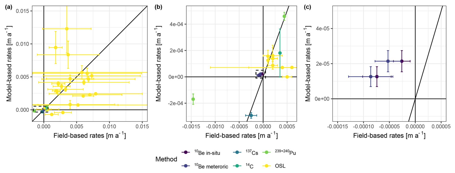
Figure 7 Point-based comparison of erosion (negative) and deposition rates (positive) for experimental, field-based data and model simulations for the corresponding locations in the landscape. The rates are represented with mean and 1σ errors. Field-based rates were derived or calculated from their original publications (See Sect. 3.4), while model-based rates were derived from the 1000 model runs performed as uncertainty analysis. (a) Overview of all available data. (b) Close-up of the data around the origin of the graph. Location of this close-up is indicated with the dashed rectangle in panel (a). (c) Close-up on the ¹⁰Be-derived rates. Location of this close-up is indicated with the dashed triangle in panel (b). The diagonal lines represent the identity lines, where field-based rates and model-based rates are identical.

On a point scale, model-derived erosion and deposition rates provide similar values as those derived from experimental data from the same locations in the landscape over the entire range of erosion and deposition rates (Fig. 7). For the OSL-derived rates, most field-based and model-based rates fall within 1σ or 2σ errors. There are some rates that are either overestimated or underestimated by the model. There are two samples where the model-derived rates show a different sign (erosion instead of deposition). The order of magnitude of OSL-derived rates ranges from 10⁻⁴ to 10⁻¹ m a⁻¹. ¹⁰Be-derived rates show larger deviations between model- and field-based rates. The order of magnitude is similar (10⁻⁵ to 10⁻⁴ m a⁻¹), but the sign of the field-based rates indicates erosion instead of deposition. Rates derived from ¹⁴C and ¹³⁷Cs fall within 1σ errors with their modelled counterparts. The same goes for deposition rates derived with ^239+240Pu, while erosion derived with ^239+240Pu show higher field-based rates than model-based rates. Rates derived from these latter geochronometers are in the order of 10⁻⁴ to 10⁻³ m a⁻¹.

4.4 Uncertainty analysis

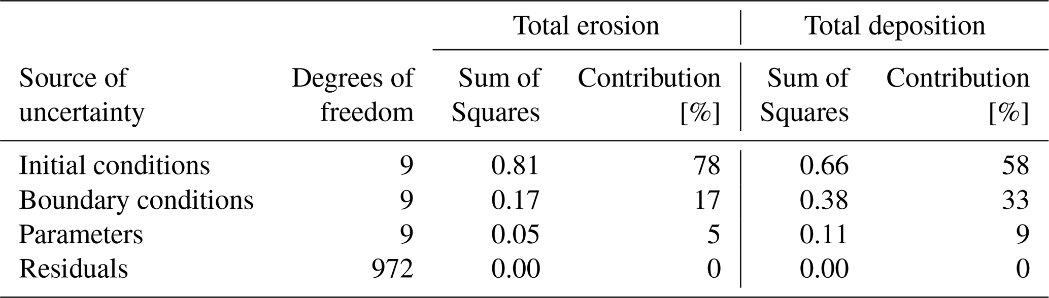
The uncertainty band around the erosion and deposition rates has a relatively constant width through time, except during the switch from one plough regime to the next, which is especially evident for the uncertain transition from ard to Medieval mouldboard period (Fig. 6a). On average, the relative standard error is about 11 % of the erosion and deposition rates. According to the ANOVA (Table 3), variation in initial conditions explains the majority of variance in the total erosion rates (78 %) and total deposition rates (58 %).Variation in boundary conditions and parameter sets contribute to a smaller degree to the variance, but play a larger role in explaining the variance in total deposition (33 % and 9 %) compared to total erosion (17 % and 5 %). There is no residual variance in the ANOVA models.

Table 3 Results of the ANOVAs to test the contributions of each source of uncertainty to the variance in total erosion and total deposition. Both tests were significant with P values ≪ 0.001. The contributions to the total variance were calculated by dividing the Sums of Squares by the total Sum of Squares.

The sources of uncertainty also show different temporal patterns. Variation in initial conditions mainly affect uncertainty in erosion rates at the start of the simulations, while its effect decreases exponentially over time (Fig. 6c). Variation in boundary conditions shows some initial variation that also decreases exponentially, before it increases again during changes of land-use periods. Variation in the parameter sets starts to affect variation in the predictions from Medieval mouldboard plough onwards, as the varied parameters correspond to this and subsequent periods. Variation caused by the parameter sets is overall lower than that caused by the boundary conditions.

5 Discussion

In this research I derived hillslope erosion rates from OSL-based deposition ages through inverse erosion modelling with the ChronoLorica model. I first calibrated the model on spatiotemporal OSL dates, followed by an uncertainty analysis to quantify different sources of uncertainty. Finally, I compared the modelled rates of landscape change with independent data. Several sources of uncertainty are present in this study. These sources are (i) the calibration process, (ii) model inputs such as initial and boundary conditions and model parameters, (iii) evaluation data and (iv) model formulations, simplifications and assumptions. Here, I discuss the different steps taken in this research and their outputs, how these may have been influenced by the different sources of uncertainty, and how these uncertainties could be addressed in future studies.

5.1 Calibration on spatiotemporal OSL data

In this study, I calibrated the ChronoLorica model on 27 OSL dates from Van der Meij et al. (2019), which were taken from five different locations (Figs. 1 and 2). The calibration was done using modal ages of the experimental and simulated age distributions. This works well in the case of tilled sediments, as the intensive reworking of the sediments at the source, during transport and after deposition produces well-bleached populations of particles (Van der Meij et al., 2019). In contrast, other hillslope sediments often contain unclear age signals due to poor bleaching (Fuchs and Lang, 2009) or particles with younger or older ages due to biological soil mixing (Bateman et al., 2003). By selecting the modal age of the distributions in this study, the well-bleached population of grains is targeted, while incompletely bleached or bioturbated particles were excluded. ChronoLorica accounts for post-depositional mixing in its tillage simulations as well. As a result, the simulated age distributions represented the same ages as the measured age distributions, facilitating calibration using their modal ages. For applications of the ChronoLorica in settings with poor bleaching or more intense bioturbation, it is necessary to simulate additional processes that influence bleaching and redistribution of OSL particles before a meaningful comparison with experimental data can be made. In addition, experimental and simulated age distributions may require more sophisticated statistical approaches, such as age models (Galbraith and Roberts, 2012), to derive a representative age for calibration.

There is an overall good fit between the measured and modelled ages with a mean absolute error (MAE) of 160 years, but there are also spatial differences in the calibration performance (Fig. 4). The model overestimated ages for profile BP5, and underestimated them for profile BP8, both located at the edges of the central depression. Profile BP6, located in the centre of the depression, shows a very good fit of experimental and simulated ages, with a MAE of just 7 years. The discrepancies for BP5 and BP8 could be due to the uncertainties in estimating the extent of the wet central part of the depression, which was based on the present-day occurrence of peat in the subsurface. This extent determines the start and rates of deposition in these locations, so any uncertainty in its estimation affects the timing of the deposition process. Although the extent was estimated using a high soil sampling density (Fig. 1), errors could have been introduced by interpolation of these observations or by the loss of peat in previously peated soils.

CarboZALF-D experienced a complex, multi-staged deposition history, which was identified by high-resolution temporal and spatial sampling (Van der Meij et al., 2019). Calibration on the spatially distributed OSL therefore helped capture both temporal and spatial dynamics in the deposition process, which enabled calibration of tillage parameters for distinct phases of landscape evolution. While calibration on data from a single location might have yielded a more precise calibration line, it would be based on a smaller dataset and overlook spatial variations in the deposition process, which are essential to understand the pre-historical erosion and deposition processes in CarboZALF-D. A spatially distributed sampling design, like the one used in this study, will not only help to interpret landscape evolution through interpretation of the OSL ages (e.g. Van der Meij et al., 2019), but also enhance the representativeness of the point-based OSL samples for reconstructing erosion and deposition on a landscape scale through inverse modelling. I recommend that future studies prioritize a spatially distributed sampling design over a high vertical resolution, as this can provide valuable insights in process dynamics which are otherwise overlooked.

The spatiotemporal calibration of the model resulted in three potential tillage parameters for three phases of landscape evolution. The parameters can be recalculated into the more commonly used tillage transport coefficient k_til by multiplying the tillage parameter with the plough depth and bulk density. The k_til parameters from this study align with those compiled by Öttl et al. (2024), except for the ard plough (Table 2). This discrepancy can be attributed to the fact that the compiled values are based on studies of modern-day tillage erosion, likely using more efficient ards, in steep-sloped areas, whereas CarboZALF-D has flat to moderately sloped terrain. The similarities between the other k_til values show that, through inverse modelling with ChronoLorica, limited geochronological data can provide accurate local estimates of prehistorical and recent tillage erosion parameters.

5.2 Erosion and deposition rates

5.2.1 Evaluation of model results

The inverse modelling provided spatial and temporal variations in erosion rates, based on the deposition ages derived from OSL dating (Fig. 6a). Pre-industrial catchment-averaged erosion rates were in the same order of magnitude as natural soil production rates and erosion rates under present-day conservation agriculture, but exceed erosion rates under natural vegetation (∼ 1 t ha⁻¹ a⁻¹; Alewell et al., 2015; Minasny et al., 2015; Nearing et al., 2017). Erosion rates under the modern mouldboard plough are almost an order of magnitude higher (5–10 t ha⁻¹ a⁻¹), with local extreme erosion rates ranging up to 100 t ha⁻¹ a⁻¹. These rates are consistent with erosion rates under conventional agriculture (Minasny et al., 2015; Nearing et al., 2017).

The close alignment between OSL-derived deposition rates and model-derived deposition rates (10⁻⁴ to 10⁻¹ m a⁻¹) was to be expected, as these data were used to calibrate the model and the OSL-derived rates contain a large uncertainty (Fig. 7). The simulated rates match with independent age controls as well, both on a catchment scale (Fig. 6a) as well as on a point scale (Fig. 7), over a range of different values. This is the case for low rates of long-term erosion and deposition determined with ¹⁰Be and ¹⁴C (10⁻⁵ to 10⁻⁴ m a⁻¹), as well as higher recent rates determined with fallout radionuclides ¹³⁷Cs and ^239+240Pu (10⁻⁴ to 10⁻³ m a⁻¹). It is important to note that these experimental rates also have inherent uncertainties and limitations. For instance, the models used to calculate rates from in-situ and meteoric ¹⁰Be produced erosion rates, even though the samples were taken from stable and depositional landscape positions (Calitri et al., 2019). Similarly, high erosion rates derived with ^239+240Pu were obtained from a site that was considered to be stable as well. The use of ¹³⁷Cs inventories to estimate erosion and deposition rates also face criticism, as the underlying assumptions are often unmet, particularly the estimation of reference inventories needed to calculate erosion and deposition (Parsons and Foster, 2011). While a well-designed sampling scheme could yield accurate estimates of the reference inventory (Mabit et al., 2013), this remains a source of uncertainty. Finally, geochronological samples are often taken from characteristic locations where erosion or deposition is evident, for example in locations with thick colluvium or completely eroded soils. These samples will provide relatively high erosion or deposition rates, which are not necessarily representative for the entire catchment. This is also apparent in Fig. 6a, where most OSL- and ^239+240Pu-derived rates correspond to the 95th-percentile rates, but not to the catchment-averaged rates. There is thus a risk of overestimating erosion or deposition rates when relying only on samples from these characteristic locations. Through landscape evolution modelling, these rates can be translated into catchment-averaged rates to better represent overall land degradation.

Despite these limitations, the experimental and model-derived rates have the same order of magnitude, within their margins of error. This agreement is unlikely to shift due to uncertainties associated with the reference methods and inverse modelling. Therefore, the provided erosion and deposition rates, along with their associated uncertainty, can be considered realistic rates of landscape evolution at CarboZALF-D across different land management practices and timescales.

5.2.2 Comparison of simulated erosion and deposition rates

The simulated deposition rates are almost always higher than the erosion rates (Fig. 6b), which confirms the hypothesis that the deposition rates cannot be used as proxies for erosion rates. In the period up to the artificial drainage, the ratio of deposition rates and erosion rates of ∼ 1.5 reflects the ratio between the size of the erosional and depositional areas in the catchment. This makes sense from a mass balance perspective, because the eroded material all accumulates in the depositional area in this catchment (Van der Meij et al., 2017). The artificial drainage increased the size of the depositional area by a small amount. However, the deposition-erosion ratio did not decrease in a similar manner, but instead increased up to 5. The large increase in topographic gradients towards the centre of the depression triggered re-erosion of the previously deposited material on the fringes of the depression and resulted in very high deposition rates in the previously uncultivated centre, shifting the balance between erosion and deposition rates. These high deposition rates comprise the largest part of the OSL-derived deposition rates from Van der Meij et al. (2019).

These findings indicate that indeed deposition rates do not represent hillslope erosion rates. Ratios between eroding and depositional areas could be used to recalculate erosion rates into deposition rates, but special attention should be given to other environmental factors that could affect the balance of these rates. These factors include changes in land management, shifts in erosion and deposition patterns, and the balance between sediment storage within the catchment and exported sediment, a common consideration for most other catchments.

5.3 Uncertainty analysis

Models are highly sensitive to uncertainties in their initial and boundary conditions and parameter sets, as these propagate through the model simulations and affect the accuracy of the model outcomes (Perron and Fagherazzi, 2012; Temme et al., 2017; Skinner et al., 2018). In this study, the reconstructed initial topography appeared to be the dominant source of variance in the model output (Table 3). This is in line with other soil and landscape evolution studies that found that models are more sensitive to uncertainty from initial conditions than from boundary conditions or process formulations (Perron and Fagherazzi, 2012; Keyvanshokouhi et al., 2016). The influence of initial conditions was most prominent at the start of the simulations and reduced to a low constant value as the simulations progressed (Fig. 6c). This could point to equifinality in the simulations, where different initial landscape states can result in similar end states (Peeters et al., 2006; Nicholas and Quine, 2010). This suggests that, while initial topography may not significantly influence the final topography, it plays a key role in determining the erosion and deposition rates required to reach that final state.

In this study, the boundary conditions were represented by the reconstructed agricultural history (Table 1). In landscapes with more dominant water erosion, the model would also require reconstructed climate and precipitation as input. This will introduce additional uncertainty as these reconstructions are often very uncertain as well (e.g. Mauri et al., 2015), which might shift the balance between the contribution of initial and boundary conditions to the overall uncertainty in the model output.

The uncertainty analysis highlights the importance to represent different sources of uncertainty in landscape evolution modelling, as these uncertainties can have a significant effect on the resulting rates of landscape change. It appears to be especially important to reconstruct pre-erosion topography, as this is a major source of uncertainty. In steady-state landscapes, the current topography can be used as a proxy for historical topography, as it is not changing over time. However, this does not apply to transient landscapes, where topography and soil depths are continually adjusting to shifts in boundary conditions, such as land-use or climate change. This is particularly true in tilled systems, where diffusive transport gradually smoothens the landscape, reducing elevation differences and topographic gradients, and consequently erosion rates, over time (De Alba et al., 2004). Using the current-day topography to represent historical conditions transient landscapes may thus underestimate past erosion rates and lead to overconfidence in the model output. Depending on the landscape, initial topography can be reconstructed using soil or sediment descriptions (Vermeer et al., 2014; Van der Meij et al., 2017), by removing erosional features through topographic interpolation (Bergonse and Reis, 2015) or through backward erosion modelling (Peeters et al., 2006; Temme et al., 2011), where each method has its own challenges and limitations. Reconstruction of boundary conditions can be based on climate and vegetation reconstructions or demographic and archaeological proxies. The main challenge here is that the uncertainty increases and the spatiotemporal resolution decrease with reconstructions further back in time (Mauri et al., 2015; Li et al., 2023), and therefore may not accurately reflect conditions at a specific location. Despite these challenges, it is crucial to quantify these uncertainties in model inputs to avoid overconfidence in the model output and to communicate the inherent uncertainties clearly.

Although the uncertainty analysis in this study involved 1000 model runs, equivalent to ∼ 4000 CPU hours, only a limited amount of variation in the model inputs was explored. By simulating unique combinations of 10 variations of initial conditions, boundary conditions and parameter sets, the effects of each variation could be isolated (e.g. Fig. 6c). This functional uncertainty analysis was sufficient to capture the main sources of variability and provides valuable insights into the model behaviour within the tested parameter space. A Monte-Carlo-based uncertainty analysis, where each model run uses unique values for model inputs, could be used to further explore the range of input variability and its impact on model outputs.

5.4 Study limitations

Several assumptions and unresolved sources of uncertainty were not covered in the uncertainty analysis. These limitations and their effects on the model results are discussed here.

5.4.1 Model set-up

ChronoLorica is a reduced-complexity model, where the complex geographical system is simplified by reducing the number of processes, variables and spatial and temporal resolution of the model domain. Reduced-complexity models aim to capture the key processes, while reducing computational and data demands (Hunter et al., 2007; Marschmann et al., 2019). In the case of this study, the model works with an annual timestep, relatively large cell sizes of 5 m and simulates a simplified tillage process with lumped parameters as input in order to simulate landscape evolution over 5000 years using the available data and within reasonable calculation times.

This reduced complexity introduces uncertainties in the model output. The tillage parameter, for example, includes effects of soil properties, management type, tillage speed and direction. Other approaches separate these effects into individual parameters to better represent effects of tillage direction in relation to slope (e.g. Quine and Zhang, 2004). Although such a representation better represents the physics behind tillage and can help to develop more sustainable tilling practices, it is not possible to accurately estimate these parameters for (pre-)historical tillage erosion based on the available data and the uncertain initial and boundary conditions without the risk of overfitting the model. By providing a range of plausible tillage parameters and k_til parameters based on the calibration and land-use reconstruction (Table 2), the uncertainty in this parameter is acknowledged and considered in the simulations.

Uncertainties stemming from model formulations and simplifications can be addressed by performing ensemble simulations using different tillage erosion models, similar to studies with different landscape evolution models (e.g. Temme et al., 2011). Through such a comparison, strengths and weaknesses of different models and their formulations can be identified for different spatial and temporal scales of simulation.

5.4.2 Exclusion of part of the catchment

The CarboZALF-D catchment was split by a railroad at the start of the 20th century, isolating the southwestern part of the catchment (Fig. 1). This area, which is relatively flat and contains mostly non-eroded soil profiles (Van der Meij et al., 2017), was excluded from the simulations under the assumption that it did not contribute significantly to overall erosion and deposition rates. Most OSL sampling locations were also situated away from the railroad, ensuring they were influenced primarily by the rest of the catchment. Any contribution of the isolated part to the overall sediment budget would at most have caused a slight overestimation of pre-historical erosion rates. For rates after 1900, this effect is negligible, as the simulated catchment corresponds to the remaining catchment area.

5.4.3 Effects of water erosion

The available data at CarboZALF-D did not allow for separate calibration of water erosion in the area, even though this process likely played a role, especially when the field was fallow. Water-transported sediments would have been deposited in the same areas as tilled sediments, and later reworked by tillage activities. As a result, any evidence of water erosion in the colluvial archive is overwritten by the dominant tillage process, making it impossible to calibrate the water erosion process with the available data. Tillage erosion has been the dominant erosion process in landscapes such as CarboZALF-D, both recently as historically (Van Oost et al., 2005; Wilken et al., 2020; Öttl et al., 2024). Therefore, the results of this study should be interpreted as representing total erosion in the catchment, with tillage erosion as the primary contributor.

6 Conclusions

This study presents a modelling exercise aimed at determining (pre-)historical tillage erosion rates in a kettle hole catchment in north-eastern Germany, which has been subjected to agricultural use for nearly 5000 years. For this area, a large geochronological dataset and reconstructed initial topography and land-use history including uncertainty were available. The study has two components: (i) derivation of erosion rates from OSL-based deposition ages through inverse landscape evolution modelling with the ChronoLorica model, and (ii) an uncertainty analysis to quantify the impacts of various sources of uncertainty on the model output.

The inverse modelling provided tillage intensity parameters for three distinct phases of land use, which were in line with a global compilation of parameters from comparable studies. Erosion rates increased by nearly two orders of magnitude, from 10⁻⁵ to 10⁻⁴ m a⁻¹ during pre-historic ard ploughing, to 10⁻⁴ to 10⁻³ m a⁻¹ in recent times, with extreme rates up to 10⁻² m a⁻¹. Deposition rates were on average 1.5 times higher than the erosion rates, but increased to up to five times higher in recent times, indicating that deposition rates cannot be directly used as proxies for erosion rates. The simulated rates match well with the independent age controls, both on point and catchment scale, over a range of different values. These findings show that inverse landscape evolution modelling can provide accurate local estimates of tillage intensity, as well as realistic estimates of rates of landscape evolution for different time periods and land management practices.

The relative standard error on the erosion rates was on average 11 %. The uncertainty analysis showed that the reconstructed initial topography had by far the largest effect on total model variance, followed by the reconstructed land-use history and the calibrated tillage parameters. This underscores the importance of reconstructing these initial and boundary conditions for an accurate representation of uncertainty in model predictions and to prevent overconfidence in the model results.

Overall, this study demonstrates the suitability of ChronoLorica for upscaling geochronological data in space and time and for assessing sources of uncertainty in landscape evolution modelling. The model provides a comprehensive framework for estimating temporally varying erosion and deposition rates in transient landscapes.