Curvature-based pebble segmentation for reconstructed surface meshes

Accurate segmentation of pebbles in complex 3D scenes is essential to understand sediment transport and river dynamics. In this study, we present a curvature-based instance segmentation approach for detecting and characterizing pebbles from 3D surface reconstructions. Our method is validated using high-resolution full 3D models, allowing for a quantitative assessment of segmentation accuracy. The workflow involves reconstructing a sandbox scene using available open-source or commercial software packages; segmenting individual pebbles based on curvature features; and evaluating segmentation performance using detection metrics, primary axes estimation, 3D orientation retrieval, and surface area comparisons. Results show a high detection precision (0.980), with segmentation errors primarily attributed to under-segmentation caused by overly smooth surface reconstructions. Primary axis estimation via bounding box fitting proves more reliable than ellipsoid fitting, particularly for the A and B axes, while the C axis remains the most challenging due to partial occlusion. 3D orientation estimation reveals variability, with cumulative errors ranging from less than 5° to more than 45°, highlighting the difficulty in retrieving full orientations from incomplete segments. Surface area metrics indicate that our approach prioritizes precision over recall, with 9 out of 10 test pebbles achieving intersection-over-union values above 0.8. In addition, we introduce a Python-based segmentation tool that provides detailed morphological and color-based metrics for each detected pebble. Our findings emphasize the potential of 3D analysis over traditional 2D approaches and suggest future improvements through refined segmentation algorithms and enhanced surface reconstructions.

1 Introduction

The characteristics of eroded material on hillslopes, river channels, and sedimentary deposits inform us about the physical, biological, and chemical mechanisms of sedimentary transport. Tectonic, climatic, hydrologic, and geomorphic driving forces generate a given size and shape distribution. By studying these distributions in time and space, we can gain insight into universal processes across different scales (e.g., Domokos et al., 2015, 2020; Szabó et al., 2015; Novák-Szabó et al., 2018). In particular, there is great interest in the size and shape distribution of pebbles in gravel-bed rivers, which can unravel downstream fining processes (e.g., Paola et al., 1992; Ferguson et al., 1996; Domokos et al., 2014; Miller et al., 2014; Lamb and Venditti, 2016), help us manage resources (e.g., Kondolf and Wolman, 1993; Kondolf, 1997; Grant, 2012), and calibrate transport and erosion models (e.g., Sklar et al., 2006; Attal and Lavé, 2006).

Accurate empirical measurements are paramount when studying pebbles. In traditional grain sieving, a sample of the local population is passed through progressively finer sieves, and the weight of the sample left behind on each sieve is measured. Then, the relative weight of each sieve-determined size class is converted into a percentage of that size. Considering the pebbles as approximating ellipsoids, this size is defined by the long a axis or intermediate b axis, and conversion factors from square holes are used to retrieve axes parameters (Bunte and Abt, 2001). The main alternative to sieving is manual measurement with rulers or calipers (e.g., Wolman, 1954; Wohl et al., 1996). Manual measurement with calipers provides a continuous distribution of grain sizes but requires subjective determination of axis length in the field by an operator and is generally a time-intensive process leading to small sample sizes. Particle templates are sometimes used instead of calipers, which can increase speed but, again, lead to binned measurements (Bunte and Abt, 2001).

Recently, (semi-)automated image segmentation (e.g., Detert and Weitbrecht, 2012; Buscombe, 2013; Purinton and Bookhagen, 2019), sometimes referred to as photo-sieving (Ibbeken and Schleyer, 1986), has become a popular alternative to manual measurement. For 2D image segmentation methods (as opposed to image texture methods; cf. Purinton and Bookhagen, 2019), it is typical to use the ellipse model to retrieve a and b axes (e.g., Graham et al., 2005). These methods can lead to much larger sample sizes in far less time than manual measurement (e.g., Purinton and Bookhagen, 2021), but this is complicated by partially buried material, lighting, irregular pebble shapes, and image quality, all leading to high uncertainties (Graham et al., 2010; Purinton and Bookhagen, 2021; Chardon et al., 2022; Mair et al., 2022). Many recent studies have also explored the utility of machine learning (convolutional neural networks) for measuring pebbles on 2D imagery (Buscombe, 2020; Soloy et al., 2020; Takechi et al., 2021; Lang et al., 2021; Chen et al., 2022; Mair et al., 2024), but these techniques require significant calibration and training data, and their universal applicability is yet to be determined. Furthermore, we note that any pebble shape determination on a 2D projected plane will likely suffer from an additional bias introduced by tilting the pebble, such that the c axis is not pointing directly upwards (cf. Fig. 1).

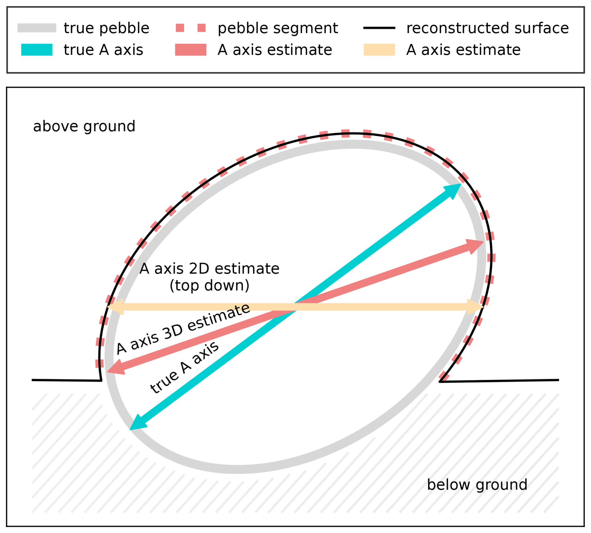
Figure 1 Schematic cross section (side view) highlighting the differences between 2D and 3D A-axis estimates and the true A-axis length. By design, a 2D estimate will underestimate the axis length as soon as the true axis is tilted. However, a 3D estimate can underestimate the axis length as well if crucial parts of the pebble are below the ground or not well reconstructed.

Pebble shapes are determined from simple a-, b-, and c-axis ratios (Krumbein, 1941); descriptors like platy, bladed, or elongated (cf. Bunte and Abt, 2001); and equations based on axis measurements (e.g., sphericity $=(b\cdot c/a^{\mathrm{2}}{)}^{\mathrm{1}/\mathrm{3}}$; Bunte and Abt, 2001). However, such metrics are based on the ellipsoid model, which reduces the entire shape of the pebble to three-axis measurements and may also be prone to uncertainty caused by subjective manual measurements or the 2D projection bias of the tilted grain. The ellipsoid model does not take advantage of the full, irregular pebble surface. Some authors have expanded on axis measurements to look at roundness and curvature of the pebble surface but often measured in a 2D image projection (e.g., Durian et al., 2007; Roussillon et al., 2009; Miller et al., 2014; Cassel et al., 2018) and less frequently from a 3D model (Hayakawa and Oguchi, 2005; Domokos et al., 2014; Fehér et al., 2023). The proliferation of point-cloud data in geosciences, spurred on by the widespread adoption of low-cost structure from motion with multi-view stereo processing (SfM-MVS; Smith et al., 2015) of photographs, has ushered in a new age of 3D environmental analysis (Eltner et al., 2016). Whereas lidar point clouds may be expensive and/or time-consuming to collect and require co-registration of different views, point clouds from SfM-MVS can be quickly gathered with a consumer-grade camera and provide a 3D triangle mesh model of the object from various sides without the need for point-cloud co-registration (cf. Fig. 2). However, the accuracy of SfM-derived point clouds or triangle meshes depends on several parameters, including image quality, image direction and orientation, number of images, and image contrast (Smith et al., 2015; Carrivick et al., 2016). An assessment of the accuracy of the SfM point cloud for millimeter-scale pebble measurements has not been performed but is required to assess measurement-related uncertainties. In this study, we estimate the necessary number of photos for a surface reconstruction with sub-millimeter accuracy.

Point clouds and triangle mesh surfaces allow accurate axis measurements by avoiding the 2D projection bias and allow measurement of additional 3D parameters in addition to axis lengths, like volume and surface area, which cannot be calculated in 2D.

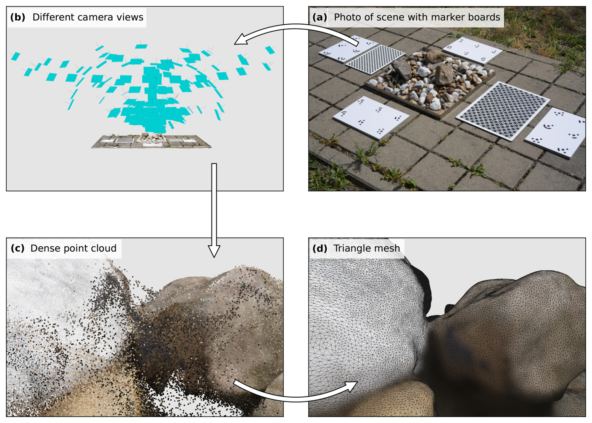
Figure 2 Reconstructed high-resolution triangle mesh as a 3D pebble model using structure from motion (SfM). (a) Overview photo of the entire scene that is also used in the SfM reconstruction. (b) Visualization of all camera views used. (c) Resulting high-resolution unfiltered dense point cloud and (d) the corresponding triangle mesh, zoomed in to reveal the individual triangles.

Point clouds have already been used to measure grain size on riverbeds but primarily via their texture, or roughness, which can be related to average grain size rather than a full distribution (e.g., Brasington et al., 2012; Rychkov et al., 2012; Westoby et al., 2015). An exciting prospect is the segmentation of individual grains from a mesh or point cloud, allowing for a partial 3D model of every visible pebble down to a measurement limit determined by the model accuracy. Walicka and Pfeifer (2022) presented a method based on random forest classification and then clustering to segment grains, and Steer et al. (2022) presented a method that segments the point cloud into watersheds to obtain grain boundaries. These methods provide reasonable segmentation results, although both have several parameters that must be set, and the performance remains qualitative.

We are motivated by these developments to present another approach and algorithm for 3D segmentation for grain-size analysis based on triangle meshes. A mesh is a network structure consisting of vertices connected by triangle edges. The vertices are XYZ point positions in 3D space, and together with corresponding triangles a continuous surface is defined explicitly. This also circumvents common pitfalls in the estimation of surface normals. Each triangle has a well-defined surface normal, and typically vertex normals are then computed by the average of all normal vectors of triangles touching that vertex. Meshes are an inherent output product of SfM processing and provide a convenient data structure for high-resolution surface analyses. In this study, we propose segmenting pebbles from a reconstructed scene based on the mean curvature of the corresponding triangle mesh, which we derive via the divergence of normals (cf. Fig. 3). Each triangle in a triangle mesh is a plane with a well-defined normal vector. Although pebbles are not always fully convex, they are well bounded by concave parts in reconstructed surfaces. This is the key assumption in our segmentation approach (see Sect. 2.4).

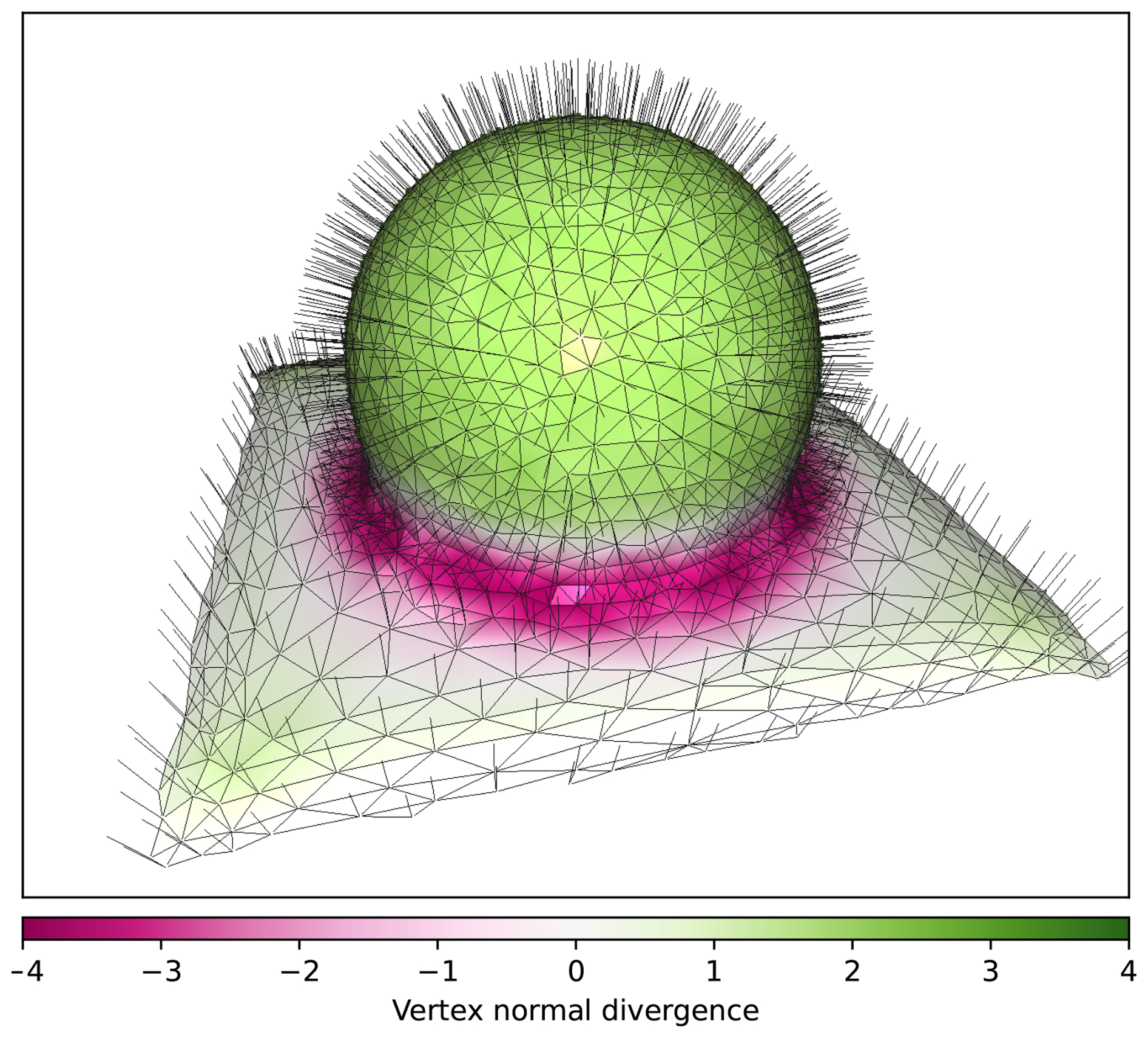
Figure 3 Coarse triangle mesh of a sphere partially buried in a flat surface. Each triangle is connected to three vertices with vertex normals. The mesh is colored by the vertex normal divergence, with diverging or convex parts being in shades of green, whereas converging or concave parts are colored in shades of purple.

2 Material and methods

2.1 Material

For our experiments, we used a 0.5 m × 0.5 m stainless steel sandbox filled with fine sand obtained from a hardware store. To facilitate accurate scaling and alignment of the reconstructed 3D models, we placed calibration chess boards and custom-made boards designed with special markers for automatic detection by Agisoft Metashape (cf. Fig. 2).

To validate the accuracy of our 3D surface reconstruction, we created a structured formation by stacking colored table tennis balls in sand in the above-mentioned sandbox. These spheres provide an ideal test case for evaluating the geometric fidelity of the reconstructed surface, as their known size and smooth curvature allow for precise error analysis.

However, the final sandbox setup consisted of a fully populated scene containing 318 pebbles with diverse color, size, and angularity (cf. Fig. 2a), including 10 numbered pebbles for which we have full 3D models. This scene represents a realistic and complex test case for evaluating our segmentation approach under natural occlusions. Photos were taken outside during daylight conditions, and no artificial light sources were used. Light-colored grains with calcitic lithologies range from 40 to 60 mm in size, while mixed quartzitic lithologies range from 16 to 32 mm in size. The surface reconstruction and segmentation results from this test form the core of our analysis. We did not rearrange the pebbles to test different packing and sorting configurations, which could be a focus for future work with the proposed segmentation algorithm.

2.2 Camera and photo capture

We used a Sony alpha6000 (ILCE-6000 v3.20) with 24MP (6000 × 4000 pixels) and a fixed 35 mm lens (Sony E 35 mm F1.8) to generate full 3D reconstructions of the 10 individual pebbles. We used the same camera for the reconstruction of the table tennis scene. We used a Sony alpha7III (ILCE-7RM3) with 42.2MP (7952 × 5304 pixels) with a fixed lens (Sony FE 35 mm F1.8) for the sandbox pebble scene. Although the Sony alpha7III has a larger number of pixels, we did not observe relevant quality differences between the 24MP and 42MP reconstructions because the images were taken from close range.

For the reconstruction of the table tennis scene and the pebble sandbox scene, we used several marker boards as a scale (cf. Fig. 2). We created A4-sized boards with 6 numbered markers that can be automatically detected by software. The distances of the markers were 12 cm in the x and y directions. We used four boards, one on each side, with a total of 24 markers to scale and orient photos. In addition to markers used by Agisoft Metashape, we used camera calibration boards by calib.io to scale reconstruction within OpenMVS and perform camera calibration experiments. We note the benefit of multiple marker boards in the scene to guide photo alignment during the SfM process and to expedite camera optimization routines.

2.3 3D surface reconstruction

Since we propose to count, measure, and characterize river pebbles in virtual reality, we need to retrieve 3D reconstructions of real scenes. This is convenient with modern open-source structure-from-motion (SfM) and multi-view stereo (MVS) software such as OpenMVG/OpenMVS (Moulon et al., 2016; Cernea, 2020) or commercial software such as Agisoft Metashape (Metashape, 2018). The software processes a set of photos from a scene of interest by performing a bundle adjustment to estimate camera parameters and positions, with a following multi-view stereo depth-map generation to retrieve a dense RGB-colored point cloud of the scene. This point cloud can also be converted to a triangle mesh, which is more useful because it provides an explicit surface. Our segmentation approach requires a triangle mesh that can be generated directly from MVS software or calculated from an existing point cloud using surface reconstruction techniques such as Poisson surface reconstruction (Kazhdan et al., 2006).

For the 3D surface reconstruction of our sandbox scene and individual pebbles, we employed an incremental structure-from-motion (SfM) and multi-view stereo (MVS) pipeline using the open-source software OpenMVG and OpenMVS. This workflow enabled the generation of dense point clouds and reconstructed meshes from input images. In the following, we outline the key steps used in the reconstruction process. The incremental SfM pipeline in OpenMVG was used to compute camera poses and a sparse point cloud. After obtaining the camera poses and sparse point cloud from OpenMVG, we performed dense reconstruction and meshing using OpenMVS's DensifyPointCloud and ReconstructMesh commands. This workflow allowed us to obtain high-resolution 3D models of both the entire sandbox scene and individual pebbles.

As an alternative, we tested the 3D surface reconstruction with the commercial software Agisoft Metashape. The quality of the output point clouds of Agisoft Metashape and OpenMVS is largely comparable, and we do not intend to provide a quality comparison. Instead, we only present an alternative approach using familiar, paid software. We note that the triangle meshes produced by OpenMVS have higher resolution, i.e., more and smaller triangles, and are therefore used throughout this study. However, for the case of many photos taken from a short distance, the differences are not important for the segmentation.

Our alternative tests rely on Agisoft Methashape (Version 2.1.2) to align, bundle-adjust, and generate dense point clouds. After photo import, we detect markers and add scale bars. Automatic marker detection allows for faster alignment of photos without accurate GNSS photo tags. We filter-detected SIFT features (called tie points in Metashape) and remove unreliable matches. We use projection error, reconstruction uncertainty, and projection accuracy to iteratively remove tie points with large covariances and generate a homogeneous covariance distribution. Bundle adjustment (camera optimization) is performed after each tie-point removal step. We calculate depth maps (or dense point clouds) only after sufficient filtering of the tie points. We emphasize the importance of a clean tie-point dataset before proceeding to the depth-map generation. The accuracy of the point cloud largely depends on an accurate estimation of camera positions, which is achieved during the bundle adjustment step.

Agisoft Metashape allows the generation of meshes directly from depth maps, and we suggest directly exporting meshes as PLY files for further processing. However, the mesh generation within Metashape performs smoothing and filtering steps to reduce the number of vertices. You may be required to customize the number of vertices that you want. If you decide to use point clouds, we suggest exporting points with normals to speed up the mesh generation step via Poisson reconstruction.

2.4 Curvature-based segmentation

Our curvature-based mesh segmentation algorithm offers an efficient approach to identifying and isolating convex parts within a 3D mesh. The process begins by computing the mean curvature for each triangle in the mesh, distinguishing between concave, convex, and flat regions (cf. Figs. 3 and 4b). Triangles with concave curvatures are discarded, leaving only those with convex or zero curvature. The retained regions are grouped into connected components (cf. colored parts in Fig. 4c) and refined through post-processing steps, such as topological hole filling, to ensure continuity and erosion to eliminate thin bridges that might otherwise connect distinct pebbles. Finally, the components are filtered based on their sphericity, removing predominantly flat segments. This ensures that the resulting segments consist of convex regions that may include flat areas but maintain an overall curved structure. These pre-processing and filtering steps make the algorithm ideal for isolating meaningful convex features in complex geometric data (cf. colored segments in Fig. 4d).

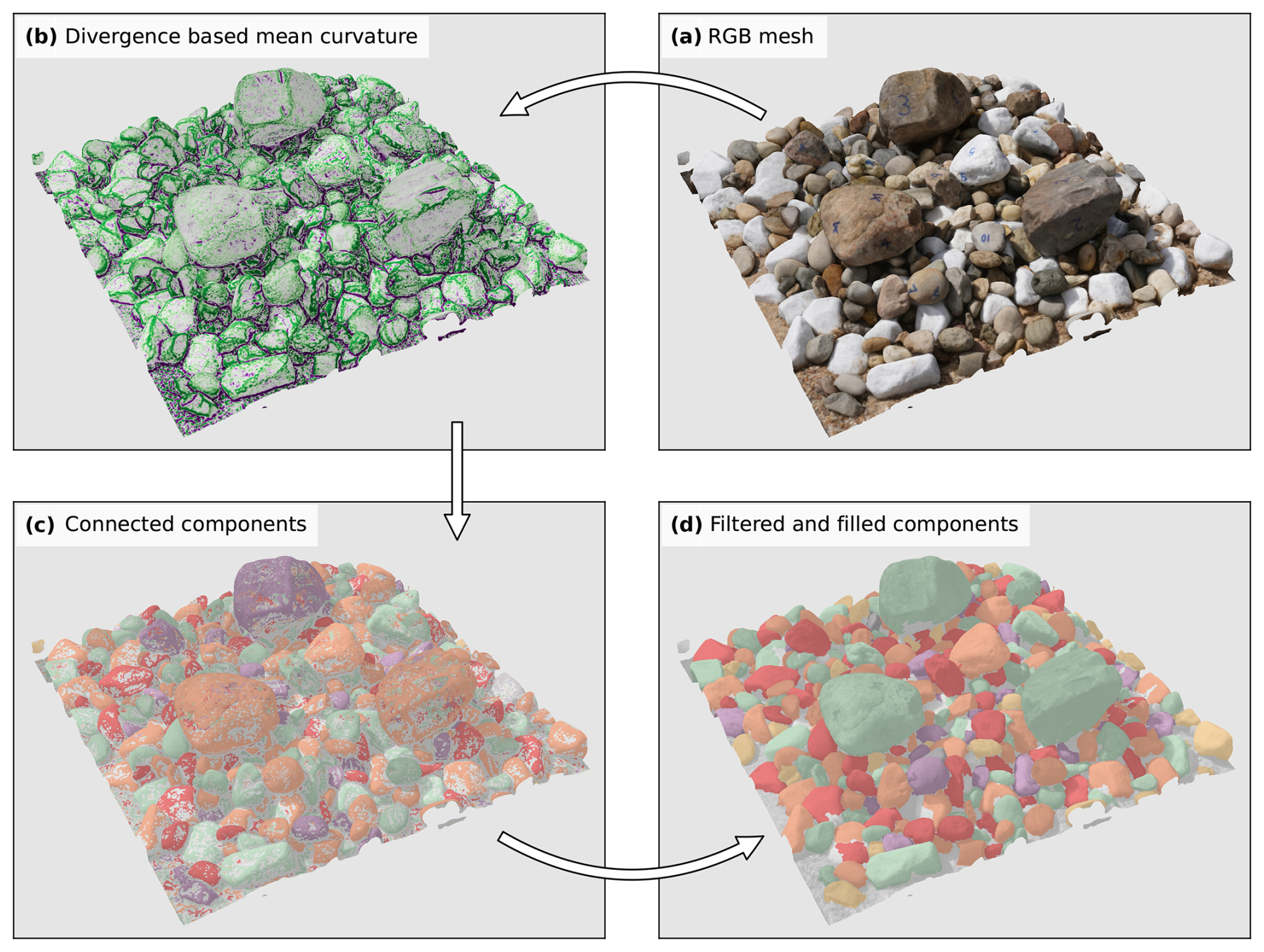
Figure 4 Workflow pipeline for the 0.5 m × 0.5 m test sandbox filled with sand and pebbles, including the 10 numbered pebbles for which we also have full 3D models that we can match into the scene. First, a 3D triangle mesh is reconstructed from RGB photos (a). RGB information is only used for visualization. Second, the mean curvature is computed from the divergence of mesh vertex normals (b). Third, all concave parts (purple) of the mesh are removed, and the remaining parts (green and white) are labeled as connected components (c). Fourth, the components are filtered based on size and sphericity, as well as topologically filled to retrieve the final pebble segments (d). Colors in (c) and (d) are only for differentiating segments.

At the core of our segmentation algorithm is an accurate and robust method for estimating mean curvature, which is derived from the divergence of the normal field (Eq. 1). Conceptually, the divergence of surface normals provides a clear distinction between surface types: diverging normals indicate convex regions, while converging normals correspond to concave surfaces. Mathematically, mean curvature H relates to surface normals n in 3D in the following way:

$$\begin{array}{}\text{(1)}& \mathrm{2}H=-\mathrm{\nabla }\cdot \mathit{n}.\end{array}$$

Our normal field, though inherently defined only on the mesh surface, is extended into the surrounding 3D space using inverse distance interpolation. The divergence at a point is computed as

$$\begin{array}{}\text{(2)}& \mathrm{\nabla }\cdot \mathit{n}={\displaystyle \frac{\partial n_x}{\partial x}}+{\displaystyle \frac{\partial n_y}{\partial y}}+{\displaystyle \frac{\partial n_z}{\partial z}},\end{array}$$

where n represents the interpolated normal field. For each vertex, the normal field around it is calculated using inverse distance weighting from nearby triangle normals. Each triangle in a triangle mesh is a plane with a well-defined normal vector. The partial derivatives for the divergence computation are estimated using finite differences, requiring offset positions along the x, y, and z axes. The offsets are automatically determined as twice the mean distance to the 25 nearest neighbors of the triangle, ensuring local adaptivity. Results are robust to changes in the number of 25 neighbors. If the number is much larger, it will introduce a smoothing of the curvature field. Generally, this number should be as small as possible while still retaining good statistics for the offset as the mean distance. This extension of the surface normal field into 3D enables a precise computation of the divergence, which serves as the basis of mean curvature H estimation (cf. Eq. 1). Finally, each vertex has its own curvature estimate, which can be extended to triangles by averaging the three vertex curvatures corresponding to that triangle, making it either convex, concave, or flat. Pebbles are mostly convex (H<0) or flat and should always have a boundary on the surface with concave mean curvature (H>0).

In our segmentation algorithm, post-processing steps such as hole filling, erosion, and dilation are implemented directly for triangle meshes, drawing inspiration from well-established concepts in mathematical morphology and image analysis. Although these techniques are widely available for image-based data, we are unaware of software that provides equivalent functionality for triangle meshes, prompting us to develop our own implementation. Here, triangles play the role of pixels, enabling these operations to be adapted to 3D geometry.

For hole filling, instead of permanently discarding triangles with concave curvature, we initially mark them for potential removal. During post-processing, holes are detected topologically by identifying connected components among the concave triangles. If a set of concave triangles is found to be touching only a single segment, it is classified as a hole in that segment and merged back with it. This ensures that holes within otherwise convex regions are accurately filled.

Erosion is performed by iteratively removing triangles from a segment if they are adjacent to other triangles already marked for removal. This approach allows for the progressive thinning of segments by peeling away layers of triangles. Dilation, the reverse process, adds triangles back to a segment if they are adjacent to the segment and were previously marked for removal. This optional step helps mitigate over-shrinking caused by erosion while ensuring that new additions do not connect previously distinct segments. These operations, tailored specifically to triangle meshes, enable precise refinement of convex segments while preserving their structural integrity and topological boundaries. For a very high quality mesh with clear and not smoothed-out curvatures between pebbles, erosion and dilation would not be required because the pebbles would be well separated by concave curvatures.

We provide the Python source code and Jupyter Notebook guides in a GitHub repository that explain pre-processing and filtering steps with multiple examples.

2.5 Validation using high-resolution full 3D models

In addition to reconstructing the entire sandbox scene containing sand and river pebbles, we also generated separate high-resolution full 3D models for 10 marked and numbered pebbles from the scene. A full 3D model is a model that represents the object from all sides. Each of these pebble models was independently reconstructed using a dedicated set of photos captured under controlled conditions. For this process, the pebbles were placed against a white background and rotated to ensure full coverage. Each dataset consisted of 66 to 158 photographs taken from very short distances, resulting in very high resolution full 3D triangle mesh models with average triangle areas ranging between 0.003 and 0.009 mm² (cf. Fig. 5).

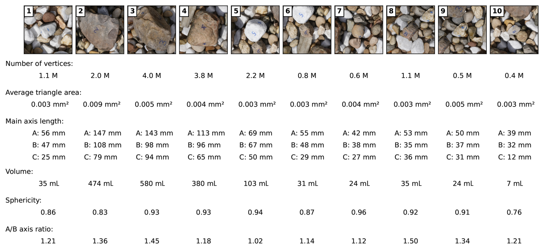
Figure 5 Overview of 10 individual reference pebbles with various characteristics of their corresponding full 3D model. These models are globally matched into the scene with all remaining pebbles and sand and can be compared to pebble segments from our algorithm. Pebbles are shown in a top-down view as being matched into the scene.

Individual pebble models exhibit a diverse range of sizes and shapes, some containing approximately half a million vertices and others reaching up to 4 million vertices (Fig. 5). This variety ensures a broad representation of the geometries, enhancing their utility as benchmarks. The primary purpose of these detailed pebble models is to align them with the reconstructed sandbox scene and to compare the retrieved pebble segments with these high-resolution full 3D models, which serve as the ground truth. This allows us to evaluate the segmentation algorithm’s accuracy in identifying and reconstructing individual pebbles within the scene.

Additionally, these full 3D high-resolution models provide an independent means of validating the overall scene reconstruction. By comparing the integrated, lower-resolution pebble representations within the scene to their corresponding high-resolution counterparts, we can further assess the fidelity of the reconstruction process. This dual-purpose approach strengthens the reliability of the reconstructed sandbox scene while offering robust ground-truth data for testing segmentation accuracy.

After segmentation of the real scene, we align these full 3D models with the reconstructed sandbox scene using the Fast-Point-Feature-Histogram-based fast global registration method (Rusu et al., 2009; Zhou et al., 2016). This alignment ensures accurate positioning of the full 3D high-resolution pebble models within the reconstructed scene, providing a reliable basis for comparison.

Once aligned, we evaluate the segmentation approach using several metrics derived from the retrieved pebble segments in the scene and their corresponding full 3D models. These metrics focus on both geometric and structural aspects, ensuring a comprehensive assessment:

• Pebble dimensions (A, B, and C axes): The primary axes of each pebble, denoted as A (longest), B (intermediate), and C (shortest), are extracted from both the segmented pebbles and the full 3D models. The comparison of these axes provides insights into the accuracy of the shape and size representation in the segmentation process.

• 3D orientation (yaw, pitch, and roll): The orientation of each pebble is evaluated using the yaw, pitch, and roll angles. These angles describe the rotation of the pebbles in 3D space and are compared between the segmented pebbles and their full 3D counterparts to assess alignment accuracy. While the full 3D counterparts are matched into the scene, their internal datum derived via principal component analysis (PCA) might vary with one of the segments due to hidden parts in the scene.

• Surface area metrics (intersection over union, precision, and recall): To evaluate how well the segmented pebble surfaces correspond to the ground truth, i.e., the high-resolution full 3D models, we compute the intersection over union (IoU), sometimes also referred to as Jaccard index. This measures the overlap between the retrieved surface area of a segmented pebble and its corresponding full 3D model, normalized by the union of both surface areas. Additionally, precision and recall are calculated to quantify the accuracy and completeness of the retrieved surface area. Precision reflects the proportion of correctly identified pebble surfaces within the segmentation, while recall indicates the proportion of the ground truth surface correctly captured in the segmentation. Note that all surface area metrics are computed in 3D and not in a 2D projection. Surface area estimations are computed at the level of individual triangles in the triangle mesh. Each triangle has a 2D planar surface area in 3D space.

For the validation of pebble dimensions, we focus on the primary axes, A (longest), B (intermediate), and C (shortest). As a first step, the A axes of the real pebbles were measured using calipers prior to their inclusion in the sandbox. These measurements were used to scale the corresponding full 3D high-resolution models, ensuring an accurate physical correspondence between the models and the real-world pebbles.

The other two axes, B and C, were estimated from the full 3D models by fitting a bounding box aligned to each model's internal datum or coordinate system (cf. Fig. 6). This coordinate system is derived from the pebble's geometry using PCA, ensuring alignment to its primary axes. For consistency, the same bounding box approach was used to estimate the A, B, and C axes of the pebble segments from the reconstructed scene. The differences between the axes derived from the segmented pebbles and those of the full 3D models were then calculated to evaluate the accuracy of the segmentation.

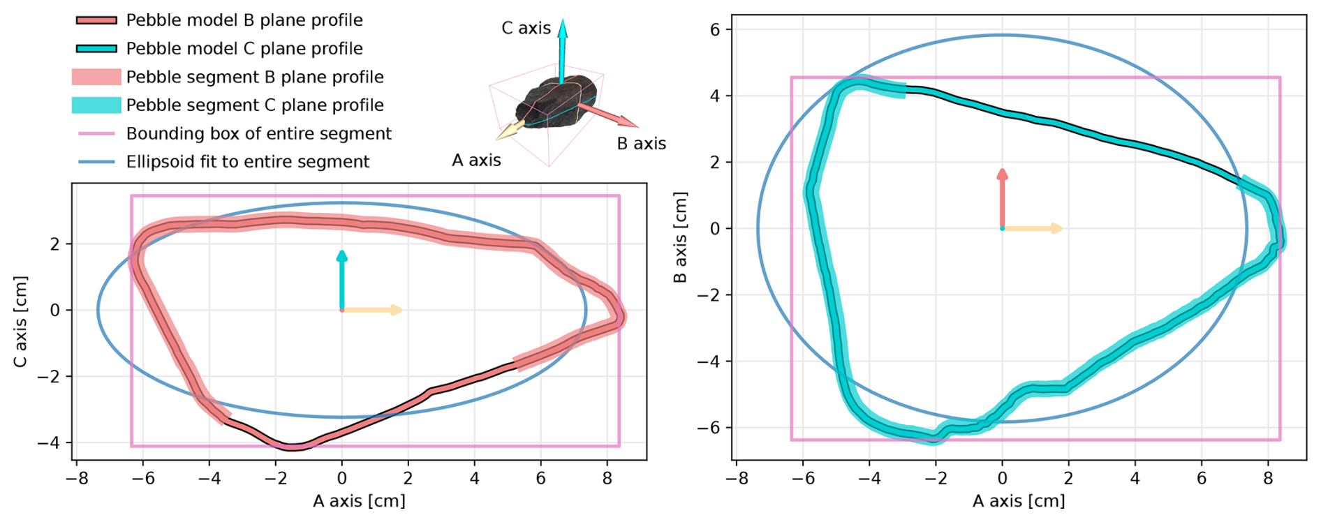
Figure 6 Illustration of the difference between the bounding box and ellipsoid-based main axis length estimation for pebble number 2. Shown are B-plane profiles on the left-hand side and C-plane profiles on the right-hand side for the segment from a reconstruction (incomplete profiles) as well as from the full 3D model.

In addition to the bounding box method, we also estimated the primary axes of the pebble segments using ellipsoid fitting, a common technique in the literature for approximating pebble dimensions (e.g., Steer et al., 2022). This method involves fitting an ellipsoid to the segmented pebble and using its semi-principal axes as proxies for the A, B, and C axes (cf. Fig. 6). However, our results show that the bounding box method generally produces more accurate estimations with lower deviations from the full 3D models.

Although pebble orientations have not been widely studied, they have the potential to reveal important information about river flow dynamics, riverbank collapses, and pebble movements. Our primary objective in this validation is to assess whether pebble orientations can be accurately estimated from typically incomplete segments of pebbles within the reconstructed scene.

To evaluate orientation accuracy, we compare the internal datum of the full 3D models with that of the corresponding pebble segments. The internal PCA-derived datum for each model and segment identifies the primary axes of the object and aligns them with a local coordinate system. This orientation of a local coordinate system (cf. Fig. 7) provides the basis for comparing yaw, pitch, and roll angles between the full 3D models and their segmented counterparts.

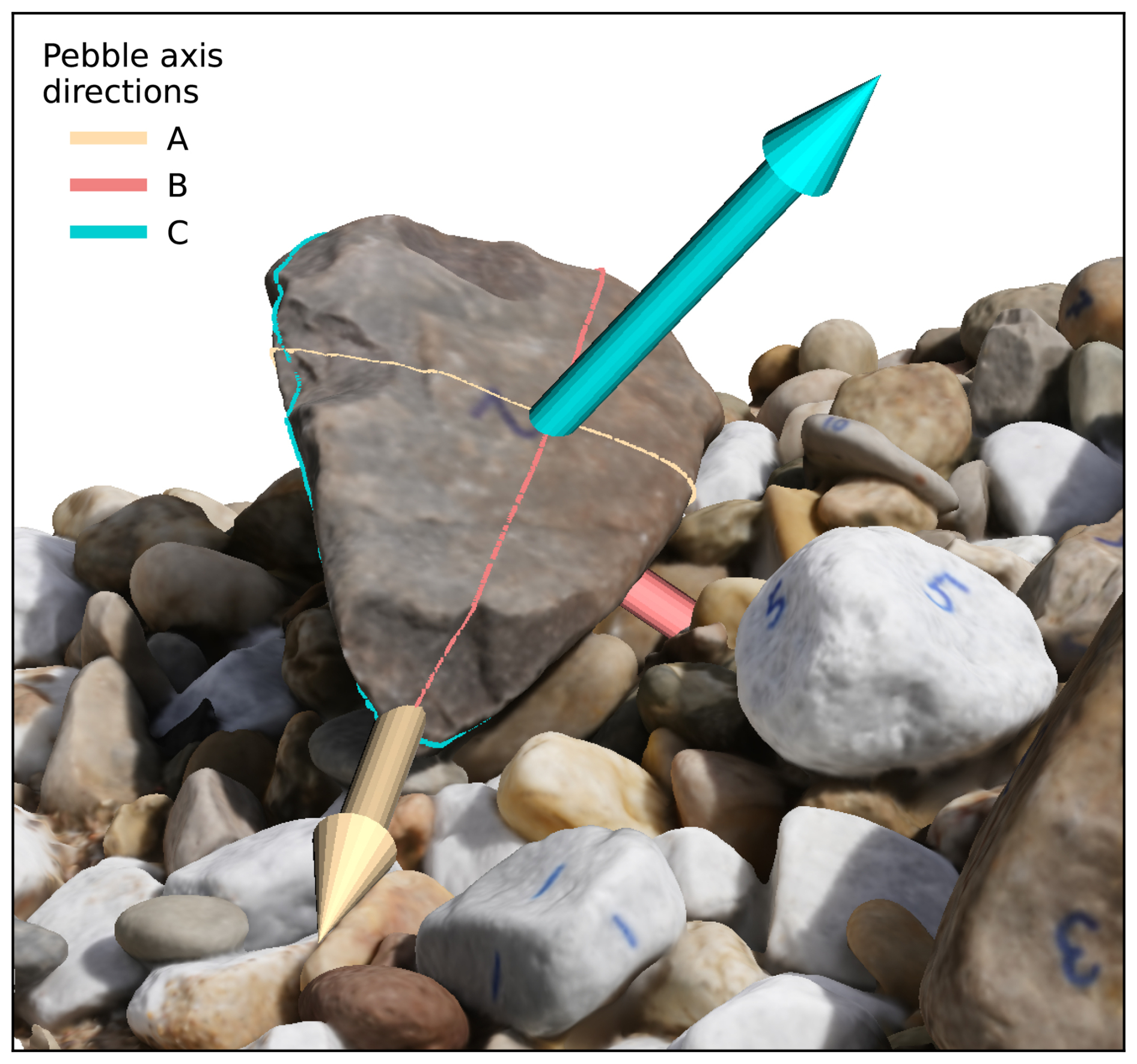
Figure 7 Illustration of pebble main axis directions and the internal datum of the pebble number 2. Pebbles can be characterized by a xyz position of the centroid, as well as the orientation of its main axes in terms of three rotations: roll, pitch, and yaw.

For the validation of our segmentation approach using surface area metrics, we also leverage the high-resolution full 3D models of the pebbles. These 10 models contain complete surface information, including portions of the pebbles that cannot be recovered from the reconstructed scene, as they may be hidden behind other pebbles or buried in sand. Consequently, our segmentation approach can only recover the visible portion of each pebble present in the scene.

To address this limitation, we first determine the retrievable part of each full 3D model by applying a distance threshold of 2 mm. This threshold identifies the triangles in the scene's mesh that are within 2 mm of the surface of 1 of the 10 full 3D models. The resulting region represents the best-case segment – the portion of the full 3D model that is theoretically recoverable from the scene. This best-case segment serves as a reference for evaluating the segmentation.

For comparison, we overlay the best-case segment with the corresponding segmented region obtained from our algorithm. Each triangle in the scene is then categorized as one of the following: true positive is a triangle that belongs to both the segmented region and the best-case segment. False positive is a triangle that belongs to the segmented region but not to the best-case segment. False negative is a triangle that belongs to the best-case segment but is missing from the segmented region.

Using these classifications and the fact that each triangle has a 2D surface area in 3D, we compute the total surface areas true positive (TP), false positive (FP), and false negative (FN) (cf. Fig. 8). From these areas, we derive the following metrics:

$$\begin{array}{}\text{(3)}& {\displaystyle }\text{precision}={\displaystyle \frac{\mathrm{TP}}{\mathrm{TP}+\mathrm{FP}}}\text{(4)}& {\displaystyle }\text{recall}={\displaystyle \frac{\mathrm{TP}}{\mathrm{TP}+\mathrm{FN}}}\text{(5)}& {\displaystyle }\text{IoU}={\displaystyle \frac{\mathrm{TP}}{\mathrm{TP}+\mathrm{FP}+\mathrm{FN}}}.\end{array}$$

Figure 8 Schematic cross section (side view) of a pebble segment and its reconstructed surface area, highlighting the true positive region (TP), false negative region (FN), and false positive region (FP), from which precision, recall, and intersection over union (IoU) are calculated.

This evaluation framework ensures that the performance of our segmentation approach is rigorously assessed in terms of its ability to accurately recover the retrievable portion of each pebble. By comparing these metrics across multiple pebbles, we can quantify both the strengths and limitations of the segmentation algorithm and identify areas for potential improvement.

3 Results

3.1 3D scene reconstruction accuracy

Although modern digital cameras capture photos in unprecedented detail, 3D scene reconstructions will never be perfect. For segmenting and measuring pebbles, it is important to know how accurate a reconstruction is, what parameters influence the quality, and how. For a control on that, we prepared a 0.5 m × 0.5 m steel sandbox with sand and table tennis balls. In total, we took 68 photos of that sandbox from various angles (cf. Fig. 9). From this set of photos, we made three separate reconstructions: one with only 8 of the top-down view photos (cf. Fig. 10a), another with 18 of the still relatively top-down view photos (cf. Fig. 10b), and a third with all 68 photos (cf. Fig. 10c). We apply our segmentation routine for all three reconstructions and generate a single triangle mesh for each table tennis ball. Since table tennis balls are manufactured as spheres with a radius of exactly 20 mm, the geometry is known precisely, and we can compare segments from reconstructions. We compare by least-squares fitting the model of the sphere to each triangle mesh segment, which provides us with a radius for every vertex of that mesh segment. We use those to calculate a distribution of radii for each reconstructed table tennis ball (cf. Fig. 10). The more narrow and centered the distribution is around the true radius of 20 mm, the better.

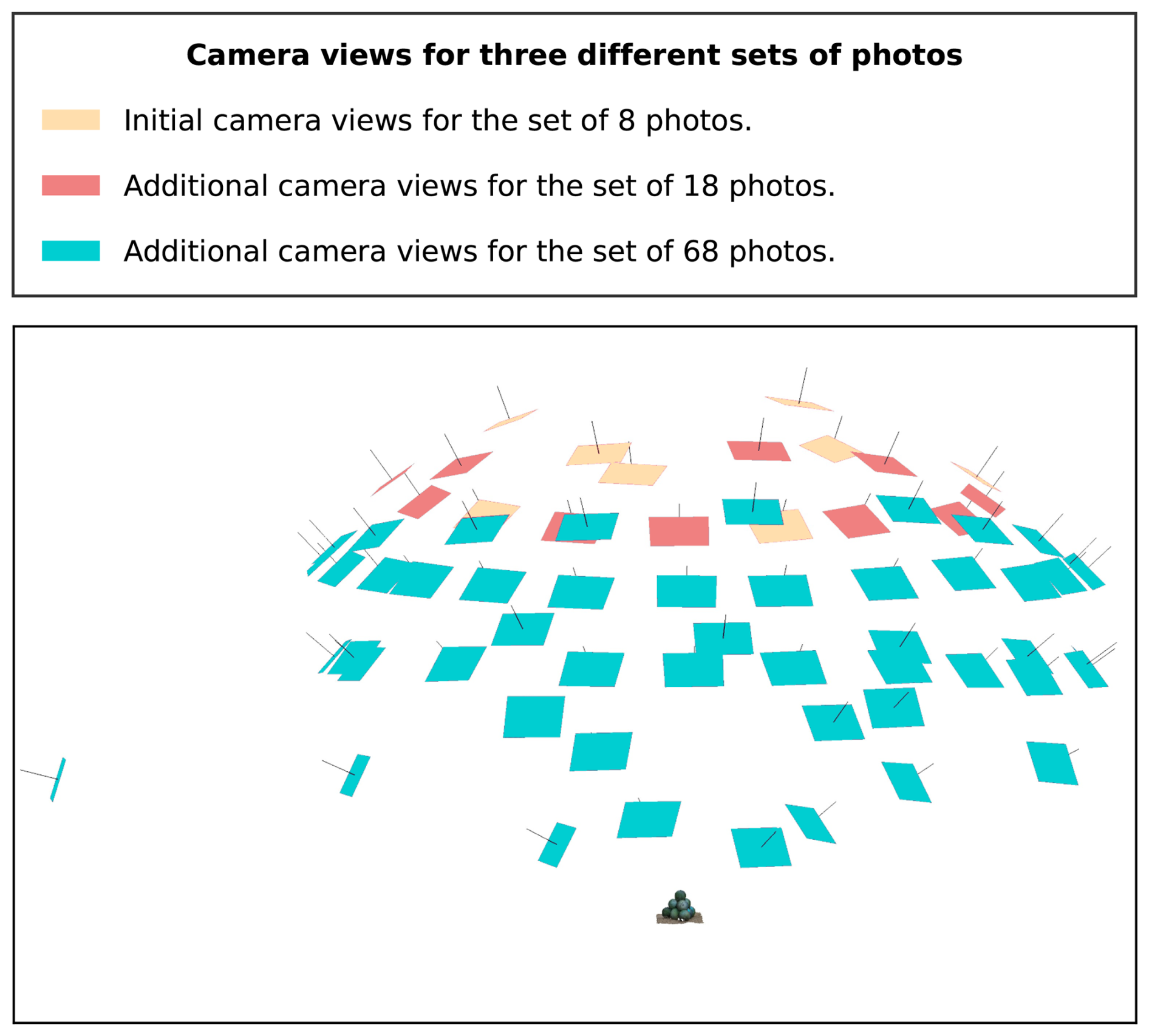
Figure 9 Visualization of the 68 different camera views for the table tennis validation setup. Photos are grouped into three sets for the analysis of reconstruction accuracies. Although top-down views are crucial, additional, more oblique views can increase the reconstruction accuracy tremendously (cf. Figs. 10 and 11).

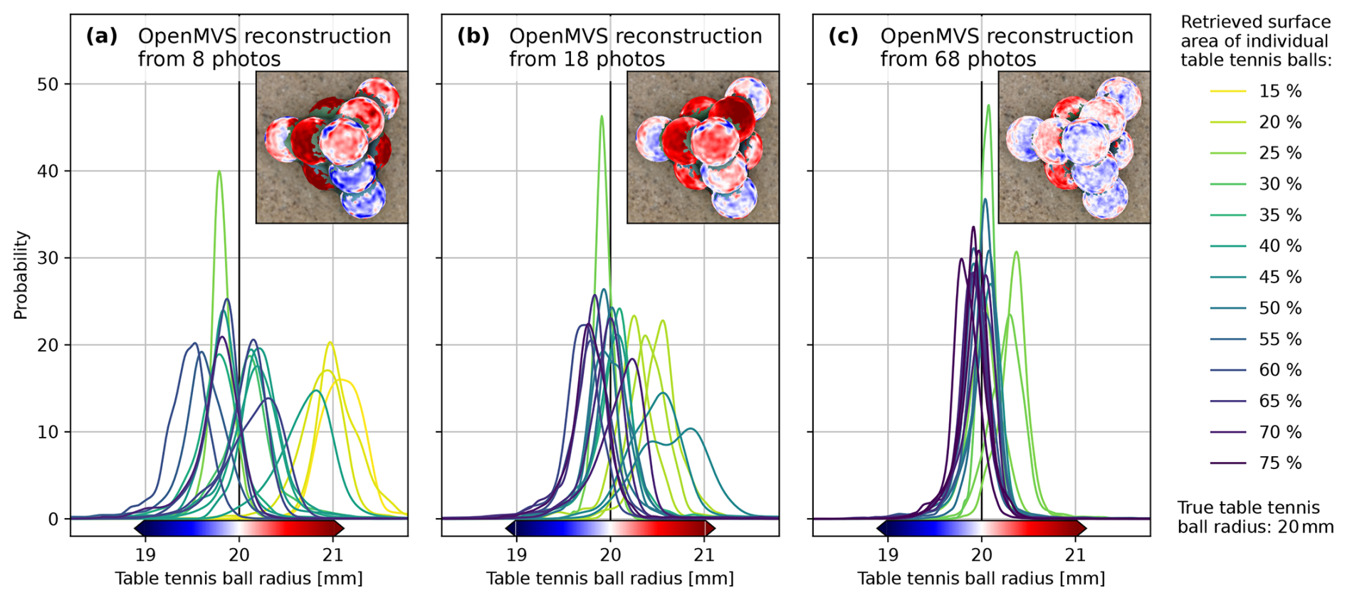
Figure 10 Reconstruction accuracy calculated for the number of photos used. Results for 8 (a), 18 (b), and 68 photos (c) from a real scene with 17 table tennis balls with radius 20 mm. All are individually segmented using our approach, and mesh vertices of a segment are used to least-squares fit the model of a sphere. Depending on the residuals of this model, each vertex corresponds to a slightly different radius, leading to a distribution of radii for each segment. These radius distributions are shown in shades of yellow to blue depending on the retrieved surface area of the true, full table tennis ball. The most complex part of the scene is a stack of 10 table tennis balls, shown in insets. Here, segments are colored according to radius residuals. The more photos used, the smaller the residuals, and the more narrow and centered around the true radius of 20 mm the radius distributions get. For 68 photos, most radii are well constrained within the interval of 20.0±0.5 mm, constituting an uncertainty of about 2.5 %.

As expected, reconstructions are more accurate if more photos with varying perspectives are used. This is reflected in a more accurate confirmation of the radii of table tennis balls with more photos. For a maximum of 68 photos, all radius distributions are more or less centered around 20 mm and well confined between 20.0±0.5 mm. The accuracy can also be quantified by the root mean square error (RMSE) of the radii of the table tennis balls. With 8 photos from near-nadir positions, a single table tennis ball has an RMSE of above 1 mm; for 68 photos, all table tennis ball radii are well confined with an RMSE of below 0.4 mm; i.e., RMSE is below 2 % (cf. Fig. 11).

Overall, this makes photogrammetry a viable option for 3D surface reconstruction of river pebbles if the density of photos matches the required accuracy. In our segmentation application scene of the same sandbox filled with sand and pebbles, we use 157 photos for 3D surface reconstruction. Hence, we can expect an even more accurate surface reconstruction compared to the table tennis experiment.

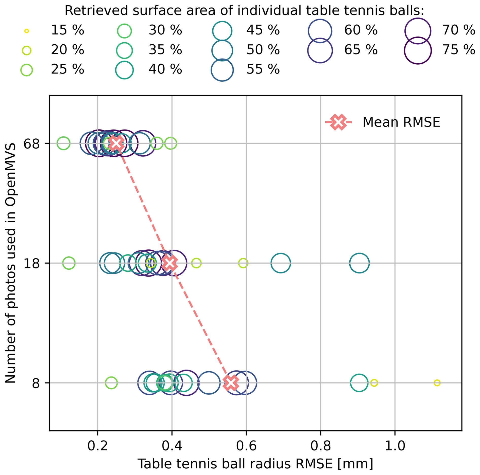
Figure 11 From the same experiment of Fig. 10 the reconstruction accuracy is shown in terms of root mean square error (RMSE) of model residuals. Each segment is represented by a circle in shades of yellow to blue. The color and size indicate the retrieved surface area of the segment. Better-represented segments tend to be closer to the mean RMSE. The latter is going down with an increase in photos used, but generally, the RMSE goes towards zero. For the best case of 68 photos, the RMSE is below 0.4 mm for all segments.

3.2 Detection of pebbles in the scene

The first segmentation result concerns the detection accuracy of all pebbles in the reconstructed sandbox scene. A pebble is considered successfully detected (true positive) if it is represented by a distinct segment (cf. Fig. 12). False positives occur due to over-segmentation, where a single pebble is represented by multiple segments, while false negatives arise from small pebbles being missed or multiple pebbles being grouped into a single segment (cf. Fig. 12 red circles).

In our reconstructed scene, which contains 318 visible pebbles, we measure 297 true detection positives, 6 false detection positives, and 21 false detection negatives. From these counts, we calculate the following metrics for detection performance:

• detection precision: $\frac{\mathrm{297}}{\mathrm{297}+\mathrm{6}}=\mathrm{0.980}$,

• detection recall: $\frac{\mathrm{297}}{\mathrm{297}+\mathrm{21}}=\mathrm{0.934}$,

• detection F1 score: $\frac{\mathrm{2}\times \mathrm{297}}{\mathrm{2}\times \mathrm{297}+\mathrm{21}+\mathrm{6}}=\mathrm{0.957}$.

These results demonstrate the effectiveness of the segmentation approach, with high precision indicating a low rate of over-segmentation and strong recall highlighting the ability to identify most pebbles in the scene.

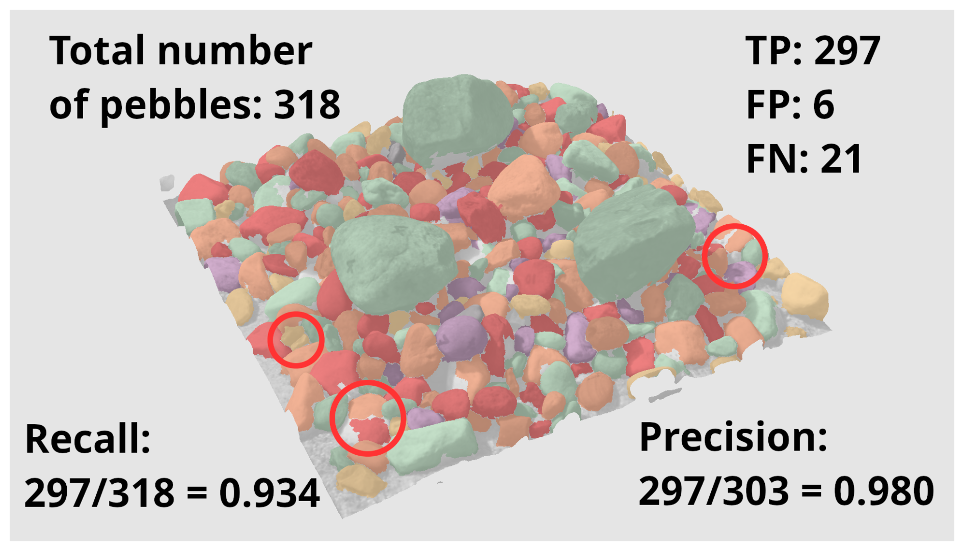
Figure 12 From this specific example scene of 318 pebbles, 297 were correctly identified (true positives, TP); i.e., 21 pebbles were missed (false negatives, FN). However, due to over-segmentation, 6 additional false pebbles were detected (false positives, FP). This gives us a precision of 0.980, a recall of 0.934, and an F1 score of 0.957. Red circles highlight a missing segment, an over-segmented pebble, and a case of under segmentation, i.e., a single segment for two pebbles.

3.3 Estimation of primary axes for full 3D pebbles

The second segmentation result focuses on the estimation of the primary axes (A, B, and C) for the 10 pebbles in the scene that correspond to our full 3D models of them. We compare two methods for estimating these axes: the bounding-box method and ellipsoid fitting (cf. Fig. 13).

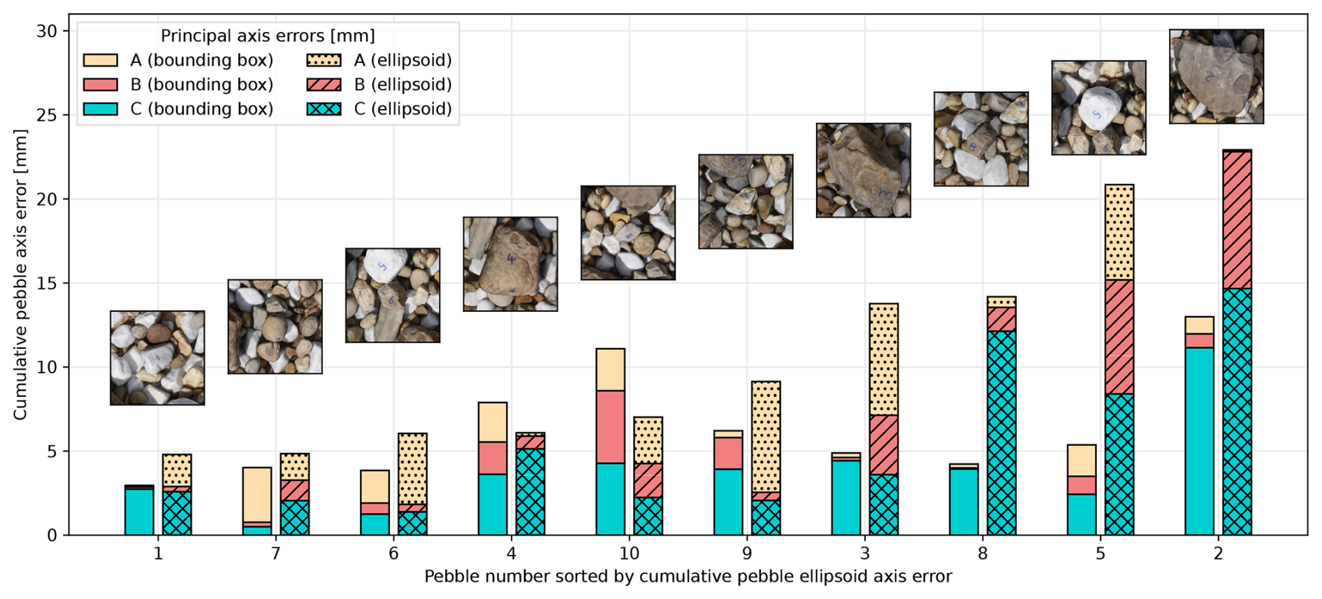
Figure 13 Comparison of ellipsoid and bounding box derived principal axis errors. For 10 archetypical pebbles, full 3D models were matched into the scan of a real scene also containing these pebbles. After segmentation and principal axis estimation from bounding boxes or ellipsoid fits, segment axes are compared to their true full 3D model axes. Axis estimations from bounding boxes are most often more accurate than those retrieved from ellipsoid fits.

When analyzing the cumulative axes errors (sum of A, B, and C errors) across the 10 pebbles, the bounding box method had lower cumulative errors compared to the ellipsoid fitting method in eight of the 10 pebbles. The smallest cumulative error was well below 0.5 cm and was achieved using the bounding box method for pebble no. 1. The largest cumulative error occurred with the ellipsoid fitting method for pebble no. 2 and was larger than 2 cm. Across both methods, errors were dominated by inaccuracies in estimating the C axis (shortest axis), indicating a consistent challenge in resolving this dimension.

These results confirm that the bounding box method provides more accurate and reliable axis estimations than ellipsoid fitting, particularly for pebbles with complex or irregular shapes.

3.4 Estimation of 3D orientations

The third result evaluates the accuracy of 3D orientation estimations (yaw, pitch, and roll angles) for the 10 full 3D pebbles in the scene (cf. Fig. 14 for an example). Orientation errors are highly variable across the pebbles, with cumulative angle errors ranging from below 5° to above 45° (cf. Fig. 15). The smallest cumulative orientation error (<5°) was observed for pebble no. 7, and the largest (>45°) occurred for pebble no. 5. Five pebbles had cumulative angle errors of 20° or less, while the remaining five exhibited larger errors.

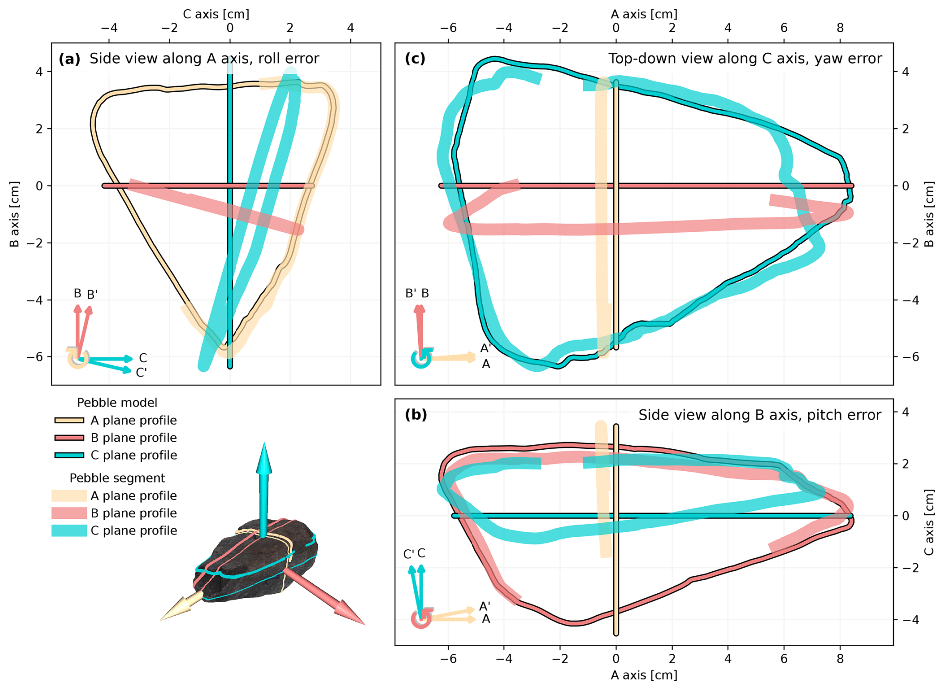
Figure 14 Orientation errors for pebble no. 2 as an example. Orientations retrieved from segments are generally different from orientations of full 3D models. We define orientation in terms of yaw, pitch, and roll angles and differences in these as orientation errors. The roll error is visible in the side view along the A axis (a), the pitch error in the side view along the B axis (b), and the yaw error in the top-down view along the C axis (c).

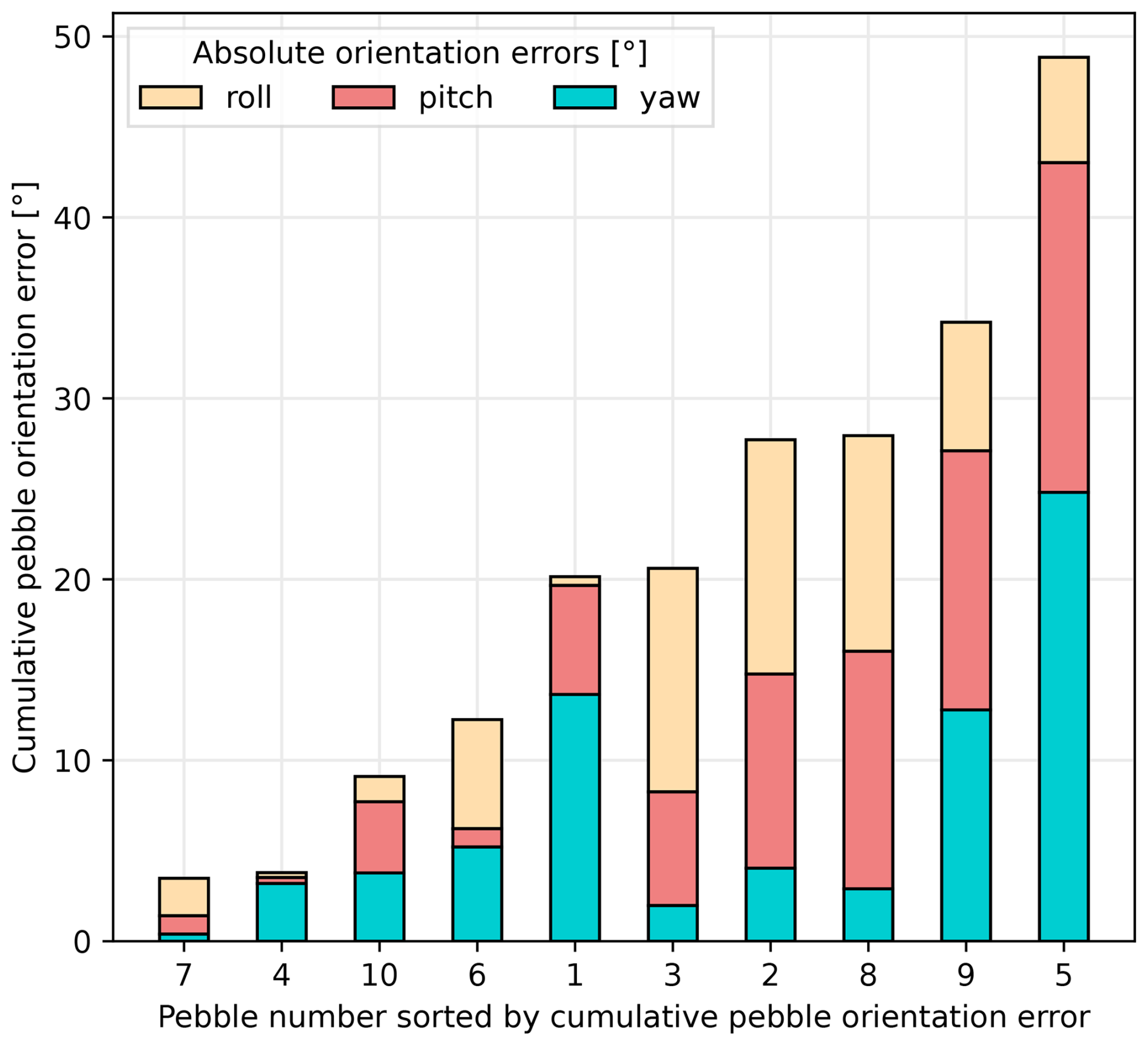
Figure 15 Cumulative absolute pebble orientation errors for the 10 numbered pebbles. While cumulative errors reach almost 50°, orientations of individual axes are always below 30°, which is about 17 % of the maximum error of 180°.

3.5 Surface area metrics

The fourth result focuses on our surface area metrics precision, recall, and intersection over union (IoU) for the 10 full 3D pebbles. Overall, the results are highly encouraging (cf. Fig. 16). For 9 of the 10 pebbles, precision, recall, and IoU values exceeded 0.8. Pebble no. 2, which had the lowest IoU, still achieved a very high precision value (close to 1), although its recall was above 0.75. If IoU values are ordered from lowest to highest, pebble no. 2 has the lowest IoU (<0.8) and pebble no. 7 the largest IoU close to 0.95 (cf. Fig. 16).

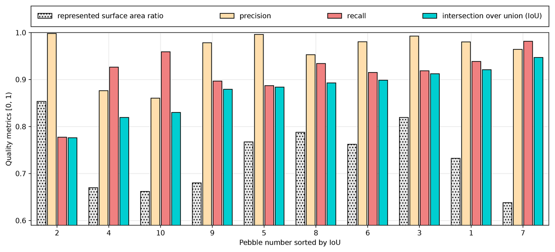
Figure 16 Segmentation quality in terms of precision, recall, and IoU of the segmented surface area versus the represented surface area in the scene. Pebbles are sorted by IoU. Not all pebbles are represented equally; some have a higher surface-area ratio than others. Although pebble no. 2 has the best-represented surface area ratio, it has the worst recall and IoU. On the other hand, pebble no. 7 has the worst surface-area ratio but the best recall and IoU.

A notable observation is that our segmentation approach tends to optimize precision over recall, as the majority of pebbles exhibit higher precision values. However, for pebbles no. 7, 4, and 10, recall values are higher than precision. Interestingly, these three pebbles also have the smallest cumulative orientation errors, suggesting a possible link between accurately recalling segments and correctly estimating orientations.

4 Discussion

Our proposed curvature-based mesh segmentation algorithm, combined with validation using high-resolution full 3D models as the ground truth, demonstrates strong potential for accurately segmenting and characterizing pebbles in complex 3D scenes. Such scenes are successfully reconstructed using structure-from-motion (SfM) and multi-view stereo (MVS) software with the required accuracy if a sufficient number of photos are taken from various perspectives. This discussion highlights key insights derived from our segmentation analysis, explores challenges, and considers implications for future applications and research.

4.1 Detection performance

The segmentation approach achieved high detection accuracy, with a precision of 0.980, a recall of 0.934, and an F1 score of 0.957 for the detection of 318 visible pebbles in the reconstructed sandbox scene. These metrics indicate that the algorithm effectively minimizes false positives caused by over-segmentation and false negatives caused by under-segmentation or missed pebbles. In particular, the number of false positives (6) is significantly lower than the number of false negatives (21). False positives are mostly due to over-segmentation, where a single pebble is incorrectly split into multiple segments. In contrast, false negatives arise from under-segmentation or missed detections, often caused by small pebbles being overlooked or multiple pebbles being merged into a single segment.

Both types of error are likely influenced by the quality of the surface reconstruction. A highly smoothed mesh of the scene leads to washed-out features, making it difficult for the segmentation approach to identify boundaries between pebbles or the boundary around a small pebble. The worse the quality of the reconstructed surface, the smoother the curvatures, resulting in a reduced segmentation performance. Addressing this limitation may require enhancing the surface reconstruction process to preserve finer geometric details.

We emphasize the need for a high-quality mesh to accurately segment pebbles. The mesh quality is mostly related to the distance the photos are taken and their direction. While drone-based acquisition with low flight height and near-nadir camera perspective will result in good orthomosaics, the 3D segmentation approach will require oblique views to capture the vertical component of pebbles. An alternative to airborne acquisition is mast-mounted cameras in 2–4 m height (Purinton and Bookhagen, 2021).

4.2 Primary axes estimation

The bounding box method outperformed ellipsoid fitting in estimating primary axes in 8 out of 10 cases, demonstrating its robustness, particularly for irregular pebble shapes. The dominance of C-axis errors in cumulative errors underscores the challenge of accurately estimating this axis, which is often the shortest and most affected by incomplete segmentation. This difficulty arises because pebbles typically rest flat in the scene, meaning their bottom portions are often obscured by sand or other pebbles. Consequently, the mesh of the scene usually only represents the top and sides of pebbles, making it harder to estimate the shortest axis.

4.3 3D orientation estimation

Estimating 3D orientations (yaw, pitch, and roll) remains a challenging task, especially when segments are incomplete due to occlusions or burial in sand. The variability in orientation errors across pebbles, ranging from less than 5° to more than 45°, reflects the sensitivity of principal component analysis (PCA)-based methods to incomplete surface data. Interestingly, there appears to be no clear relationship between pebble size and orientation errors. Instead, the variability in errors is likely influenced by pebble shape, geometry, and possibly surface area recall. Orientation and primary axis estimation errors are also not independent. The five pebbles with the largest cumulative orientation errors are also those with the largest cumulative primary axes errors. Despite these challenges, the strong correlation between high recall and accurate orientation estimation, as observed for pebbles no. 7, 4, and 10, suggests that prioritizing recall during segmentation can improve orientation accuracy. This relationship merits further exploration, particularly in the context of applications, where pebble orientation is critical for understanding sediment dynamics. The orientation estimations for some pebbles, such as no. 7, were remarkably accurate.

A key challenge in 3D orientation estimation arises from the incomplete nature of the pebble segments in the real scene. Significant portions of the full 3D models are often occluded by other pebbles or sand in the reconstructed scene, which can lead to discrepancies between the two orientation estimates. The less a pebble is exposed, the greater the orientation error. In other words, as pebble exposure decreases, orientation errors increase. Despite this, our results indicate that the orientation estimates are generally robust.

In contrast to traditional methods based on orthomosaics or 2D projections, our approach retrieves complete 3D orientations and not just one orientation angle. For example, while yaw can sometimes be estimated from orthomosaics if the C axis is perfectly aligned with the nadir, any slight tipping of the C axis leads to the underestimation of yaw. Pitch and roll are completely irretrievable from 2D data. Our method, by leveraging the internal datum derived from PCA, ensures a more accurate and comprehensive representation of pebble orientations in three dimensions.

4.4 Surface area metrics and representation

The evaluation of surface area metrics such as precision, recall, and IoU revealed that our segmentation approach tends to optimize precision over recall. For 9 out of 10 pebbles, all three metrics exceeded 0.8, demonstrating the algorithm's ability to capture retrievable segments with high fidelity. Notably, pebble no. 2, with the lowest IoU, still achieved near-perfect precision, highlighting the segmentation algorithm’s tendency to avoid under-segmentation at the expense of slightly lower recall.

Interestingly, the three pebbles with recall greater than precision – pebbles no. 7, 4, and 10 – also had the smallest orientation errors and lowest represented surface area ratios. This finding underscores the importance of ensuring that segments accurately represent the portions of pebbles visible in the scene mesh. In addition, we computed the represented surface area ratio, which measures the proportion of the full 3D pebble model that is present in the scene mesh. This ratio was lowest for the same three pebbles (no. 7, 4, and 10) that showed the smallest cumulative orientation errors. This suggests that it may be more critical for a segment to accurately recall the part of a pebble represented in the scene, rather than for the pebble to have a high surface area ratio in the reconstructed scene. Future refinements could explore adaptive thresholds for balancing precision and recall, potentially leading to improved performance across all metrics.

4.5 Example application of the segmentation software

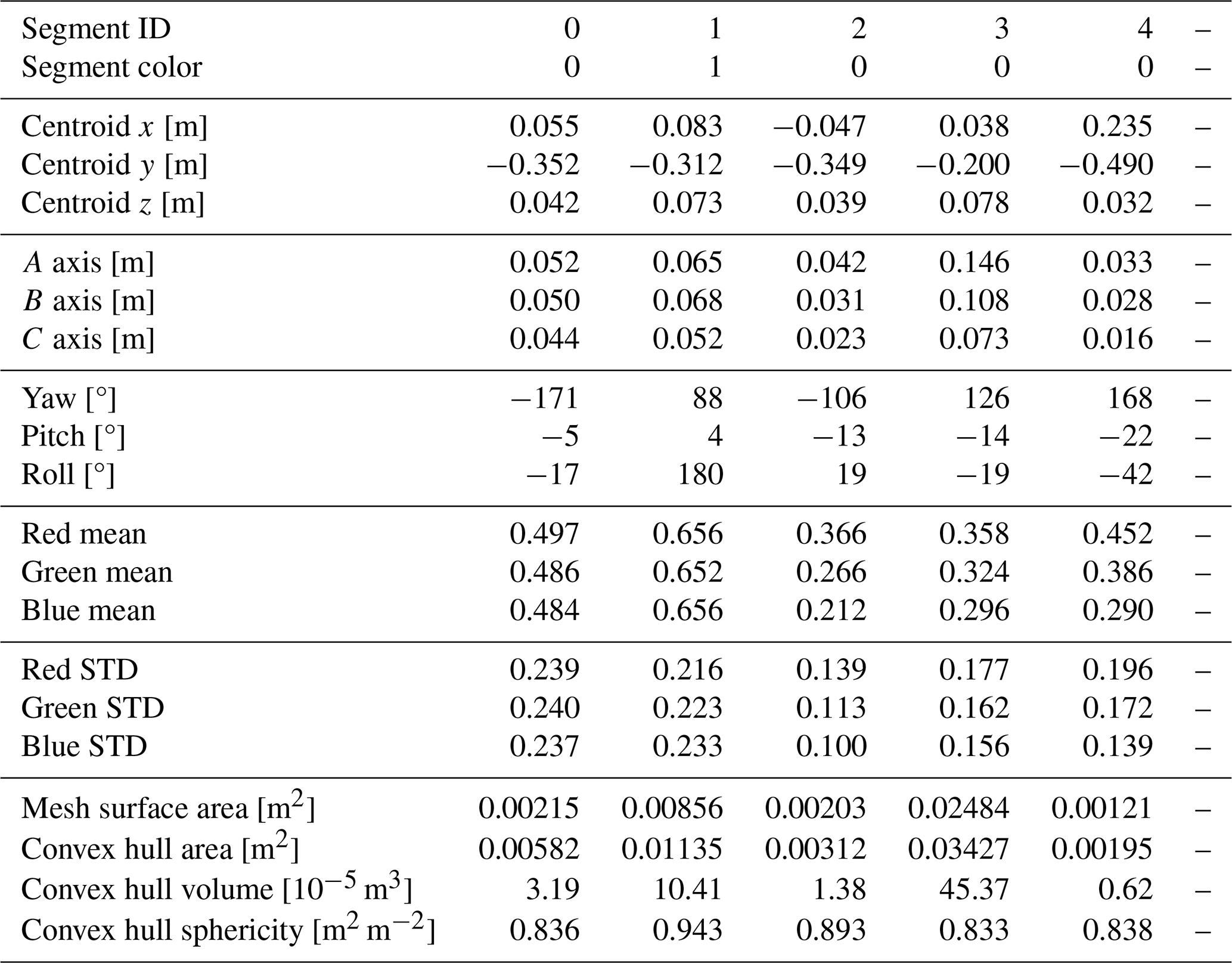
To illustrate the practical utility of our segmentation approach, we apply our Python software to the sandbox scene and demonstrate the resulting segmentation and quantitative analysis. While surface reconstructions from many high-resolution images often require hours of computation on a modern desktop computer with a GPU, our Python software for segmenting such a surface reconstruction takes less time by an order of magnitude in comparison. The software performs instance segmentation and generates a table (see Table 1) where each segmented pebble is assigned various attributes:

• segment ID: a unique identifier for each pebble;

• segment color: a locally unique identifier useful for visualization, derived via graph coloring;

• centroid (X, Y, Z): mean coordinates of the segment;

• A, B, and C axes: derived using the bounding-box method for efficiency and accuracy;

• yaw, pitch, and roll: pebble orientation in degrees;

• color statistics: mean and standard deviation values for the red, green, and blue channels extracted from the mesh;

• surface metrics: segment surface area, convex hull surface area, convex hull volume, and convex hull sphericity.

Table 1 Example output in table format from the Python software. Each segment ID denotes an individual pebble segment from our curvature-based algorithm.

As an example analysis, we estimate and visualize the distributions of A-, B-, and C-axis lengths across the segmented pebbles (cf. Fig. 17). The resulting histograms estimated using logarithmic binning highlight the variability in pebble sizes, providing insights into grain-size distribution within the scene. This example demonstrates the broader potential of our methodology, offering a detailed, automated way to extract and analyze pebble attributes from 3D reconstructions.

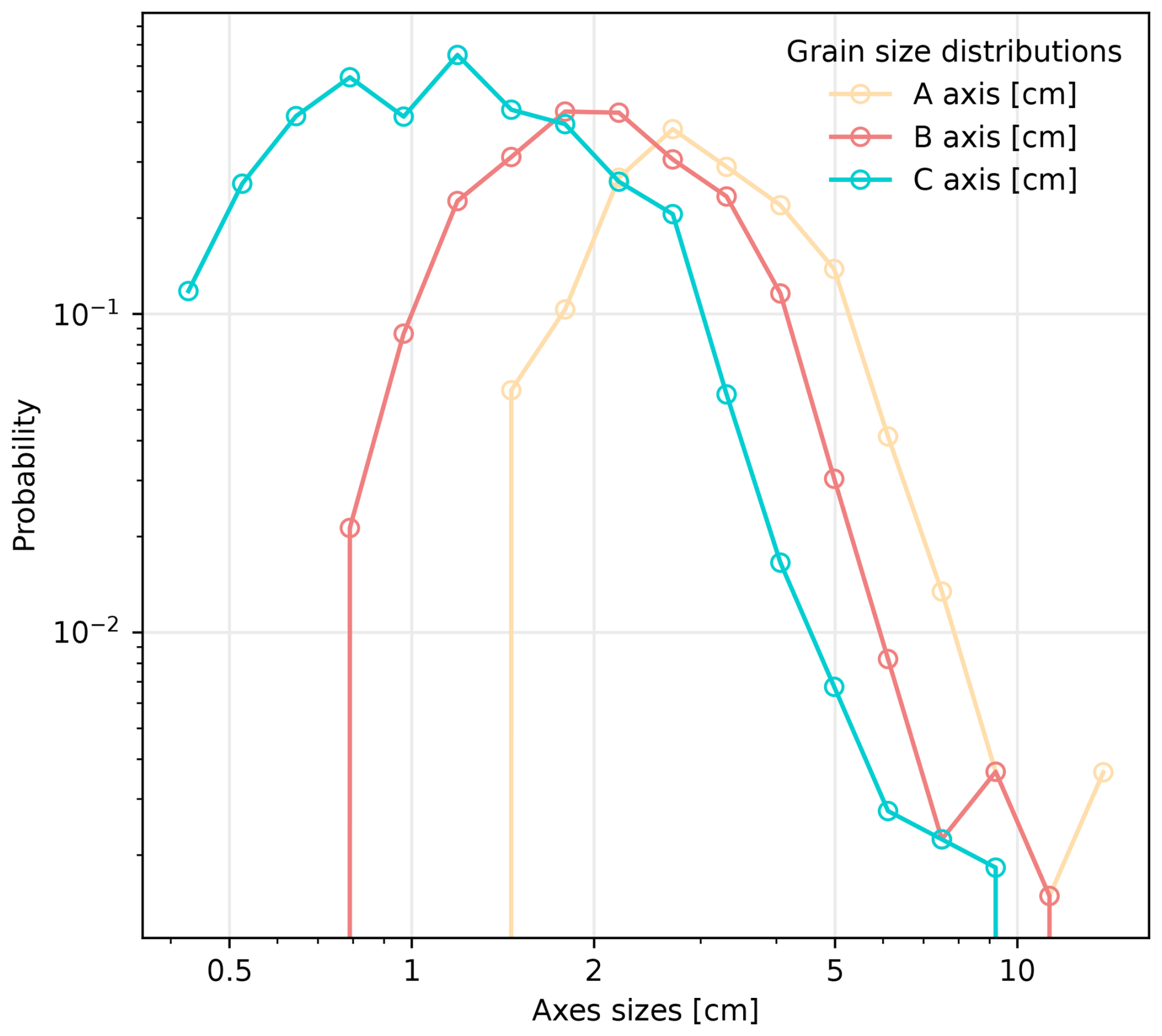
Figure 17 Example analysis of the sandbox scene and its corresponding grain-size distributions estimated by histograms with logarithmic binning for the A-, B-, and C-axes lengths as computed by our Python software and available on GitHub.

4.6 Implications and future directions

Our findings have several implications for riverine and sedimentological studies. The ability to accurately segment and characterize pebbles, including their primary axes and 3D orientations, provides valuable data for the understanding of river flow dynamics, sediment transport, and depositional processes. Additionally, the use of high-resolution full 3D models as a validation tool ensures rigorous assessment of segmentation accuracy, setting a standard for future research in this domain.

However, challenges remain, particularly in handling highly irregular shapes, small pebbles, and occlusions. Integrating complementary data sources, such as RGB color or hyperspectral information, could enhance segmentation robustness. Further, refining the algorithm’s component-based approach to segmentation could improve its ability to handle complex topologies in the mesh. In particular, more advanced techniques used in image segmentation approaches, such as random walks, will likely outperform our approach.

Finally, while our approach focuses on pebbles, its underlying principles are broadly applicable to other domains requiring curvature-based segmentation of 3D meshes, such as isosurfaces in medical imaging, size and orientation of speleothems in caves and karst, and trees in a forest. Future work could explore these applications, expanding the algorithm’s impact beyond sedimentology.

5 Conclusions

The precision of point cloud or triangle mesh surface reconstructions depends on the number of photos. With near-field photo acquisitions, we constrain uncertainties using table tennis balls to an RMSE of below 2 % in the ideal case of 68 photos. With only eight nadir photos, it is only below 6 %.

We present a Python pipeline for our curvature-based mesh segmentation to delineate individual pebbles from a 3D scene. Our test field with 318 individual pebbles inside a 0.25 m² sandbox indicates a high detection accuracy, with segmentation errors primarily linked to under-segmentation due to overly smooth surface reconstructions. Bounding-box-based primary axis estimation proves to be more reliable than an ellipsoidal fit for the A and B axes, while C-axis estimation remains challenging due to occlusions. Surface area metrics highlight the trade-off between precision and recall, with our approach favoring precision.

Compared to 2D approaches, 3D pebble segmentation provides a more complete representation of individual pebbles. 3D pebble segments allow for the estimation of all three primary axes and orientations, including the possibility of retrieving surface or volumetric parameters.

We emphasize the need for a high-quality mesh that can be derived from multiple photo views from varying angles to successfully segment pebbles. Future work should focus on refining segmentation algorithms and improving surface reconstruction fidelity to enhance accuracy and applicability.