Parameter estimation of river incision models of soft sedimentary rocks – a case study on the Kamikita Coastal Plain, northeast Japan

Understanding river incision model is crucial for predicting long-term landscape evolution. For the bedrock channel incision model (detachment-limited (DL) model: erosion rate E=KA^mSⁿ where A is drainage area, S is channel gradient), parameters (K, m, and n) can be estimated via slope-area analysis if E is known. Using ¹⁰Be denudation rate, previous studies globally compiled the parameter values for variable lithology. However, limited data availability for soft sedimentary rock restricts the applicability of global compilation. In addition, measuring the ¹⁰Be concentration in sedimentary rock is challenging in humid and tectonically active regions. To address this, slope-area analysis was conducted in the Kamikita Coastal Plain, Japan, where lithology (Miocene to Pleistocene sedimentary rocks) and uplift rate (∼ 0.2 mm yr⁻¹ for the past 300 ka) are assumed to be uniform. River incision rates were derived approximately from widely distributed marine terraces (MIS 5e–11). For six target rivers, DL-like behaviour was confirmed in the limited areas located upstream of the alluvium distribution. The reference concavity $m/n$ was 0.44 ± 0.10, typical for steady-state channels. Across the $m/n$ range of 0.4–0.6, the exponent n consistently exhibited nonlinearity ranging between 1.14 to 1.34, which is consistent with the previous global compilations. This observed nonlinearity likely reflects transient landscape responses to past sea-level changes, which generated slope-break knickpoints at similar elevations. Finally, the estimated erosion coefficient K (10⁻⁵–10⁻⁶) agreed with the global relationship with unconfined compressive strength q_u ($K\propto \mathrm{1}/q_{\mathrm{u}}^{\mathrm{2}}$), supporting the significant influences of bedrock lithology on K.

1 Introduction

Prediction of long-term landscape evolution is indispensable for social planning and infrastructure management, such as radioactive waste repositories, mine waste deposits, and landfills. In several fields, long-term assessments spanning 10⁴–10⁵ years are required to confirm geological stability; for instance, carbon dioxide capture and storage (∼ 10 000 years: IPCC, 2005; Alcalde et al., 2018) and radioactive waste disposal (100 000 years for intermediate-level waste: e.g., SSM, 2008; NRA, 2021). To ensure reliable risk assessment for these facilities, including the evaluation of future erosion depths and their effects on groundwater flow systems, past landscape evolution since the Late Quaternary (i.e., the last glacial–interglacial cycle since 125 ka) must be elucidated. Among various landscape processes, river incision is one of the main drivers of landscape evolution and can cause considerable vertical erosion (e.g., Whipple, 2004). Therefore, a quantitative understanding of river incision models and their parameters is essential for robust long-term projections of erosion depth.

River incision models are broadly classified into two types: the detachment-limited (DL) model and the transport-limited (TL) model. The DL model assumes that all particles eroded by the river are immediately removed from the system. The long-term river incision rate E [L T⁻¹] is controlled by shear stress or stream power per unit width on the bed (e.g., Howard and Kerby, 1983; Howard, 1994; Whipple and Tucker, 1999). Under idealized circumstances, E is described as a simple function of both channel slope S [–] and upstream drainage area A [L²] as follows (stream power incision model):

$$\begin{array}{}\text{(1)}& E=K{A}^m{S}^n,\end{array}$$

where m and n are positive constants ($\mathit{\theta }=m/n$ is the concavity index). K [L^1−2m T⁻¹] is the erosion coefficient reflecting the combined influences of bed erodibility, climate and downstream changes in channel hydraulic geometry. On the other hand, the TL model assumes that sediment flux Q_s [L² T⁻¹] transported by the river is limited by its transport capacity (Henderson, 1966; Hergarten, 2020):

$$\begin{array}{}\text{(2)}& Q_{\mathrm{s}}\propto A^{m+\mathrm{1}}{S}^n.\end{array}$$

The values of S and A can be easily calculated based on digital elevation model (DEM). Therefore, if E is known and the environment (i.e., tectonics, lithology, and climate) is uniform, the river incision parameters (m, n, and K) can be estimated from the field data and the DL model (e.g., Kirby and Whipple, 2012; Lague, 2014). When using data from rivers with different drainage areas, a reference concavity θ_ref, generally the regional mean of observed θ, is used for comparison purposes.

In recent decades, river incision parameters have been estimated in various regions (e.g., Kirby and Whipple, 2012; Lague, 2014; Harel et al. 2016; Hilley et al., 2019; Adams et al., 2020; Desormeaux et al., 2022; Hu et al., 2023; Marder and Gallen, 2023; Ott et al., 2023) and global compilations have been conducted using this data. For example, Lague (2014) estimated the parameters for 10 basins globally distributed and found that n ∼ 2 (ranging from 1 to 4) using θ_ref = 0.45. Harel et al. (2016) compiled the parameter values at 59 study areas of various lithology, climatic, and tectonic settings. Using θ_ref = 0.5, a mean (±1σ) n of 2.7 (±2.9) was suggested. Moreover, Haag and Schoenbohm (2025) indicated that the global compiled K in Harel et al. (2016) is inversely proportional to the square of unconfined compressive strength q_u: $K\propto \mathrm{1}/q_{\mathrm{u}}^{\mathrm{2}}$.

However, there are two problems with the above studies. First, previous research (q_u ≥ 15 MPa: Haag and Schoenbohm, 2025) lacks data of soft sedimentary rocks. This is especially important for tectonically active regions like Japan where over 50 % of the surface geology consists of Paleogene and Neogene sedimentary rocks (NUMO, 2021). Nevertheless, river incision parameters and its relationship with q_u have not been discussed for soft sedimentary rocks with q_u = 1–10 MPa. Second, previous parameter estimations have primarily relied on basin average denudation rates derived from cosmogenic radionuclides (CRN), such as beryllium-10 (¹⁰Be) in quartz grains from river sediments. However, it is difficult to measure the ¹⁰Be concentration for sedimentary rocks in humid and tectonically active regions like Japan due to the lack of quartz and the diversity of topographic deformation and sedimentation-erosion processes (AIST, 2016). In such regions, the ¹⁰Be measurement is appropriate for quartz-rich rocks, such as granite (e.g., Takahashi et al., 2023). Furthermore, CRN-derived denudation rates typically reflect relatively short-term durations, which are roughly inversely proportional to the incision rate (Lal, 1991). Therefore, CRN-derived denudation rates reflect average timescales of 10⁵ years in active regions with erosion rates of several mm kyr⁻¹, but only 10²–10³ years in tectonically active regions with several m kyr⁻¹ erosion (von Blanckenburg, 2006). Another conventional approach is to assume a topographic steady state (e.g., Snyder et al., 2000; Kirby and Whipple, 2001; Duvall et al., 2004). However, many environments have not yet attained a steady state (Bishop et al., 2005; Campforts and Govers, 2015; Vanacker et al., 2015; Armitage et al., 2018). Especially in coastal areas, the landscape has been drastically changed due to periodic sea-level change. Thus, as Lague (2014) noted, deriving locally measured incision rates from dated terraces remains one of the least potentially biased methods for quantifying long-term incision. However, only a few studies (e.g., Lague, 2014) address this issue by using reach incision rates based on strath terraces.

To address these issues, we performed slope-area analysis in the Kamikita Coastal Plain, Japan, where bedrock lithology (sedimentary rocks of Miocene to Pleistocene) and uplift rate are assumed to be uniform. Parameter values were estimated based on river incision rates approximately derived from marine terraces (Marine Isotope Stages (MIS) 5e, 7, 9, and 11) widely distributed in the area. First, we estimated the validity range of the DL model and θ for six target rivers. Then, we estimated the river incision parameters using the erosion rates approximately evaluated from the marine terraces. Finally, we confirmed the validity of the estimated parameter values by comparing them with those from previous global compilations.

2 Study area

The Kamikita Plain in northeast Japan is a vast coastal plain approximately 30 × 50 km², located along the coastline of Pacific Ocean (Fig. 1a). In this region, Middle and Late Pleistocene marine terraces are widely preserved at multiple levels (Fig. 2a): the Takadate terrace (MIS 5e), the Tengudai terrace (MIS 7), the Shichihyaku terrace (MIS 9), and the higher terrace (MIS 11) (AIST, 2016). The chronology has been estimated using various techniques: sediment rate chronology (Miyauchi, 1985; Koike and Machida, 2001), optically stimulated luminescence (AIST, 2015, 2016), and tephra and phytolith stratigraphy (Kuwabara, 2004, 2007, 2009; Matsu'ura et al., 2019). Based on these previous studies, Matsu'ura et al. (2019) concluded that the uplift rate of the Kamikita Plain (around Lake Ogawara) has been constant at approximately 0.2 mm yr⁻¹ over the last 300 ka.

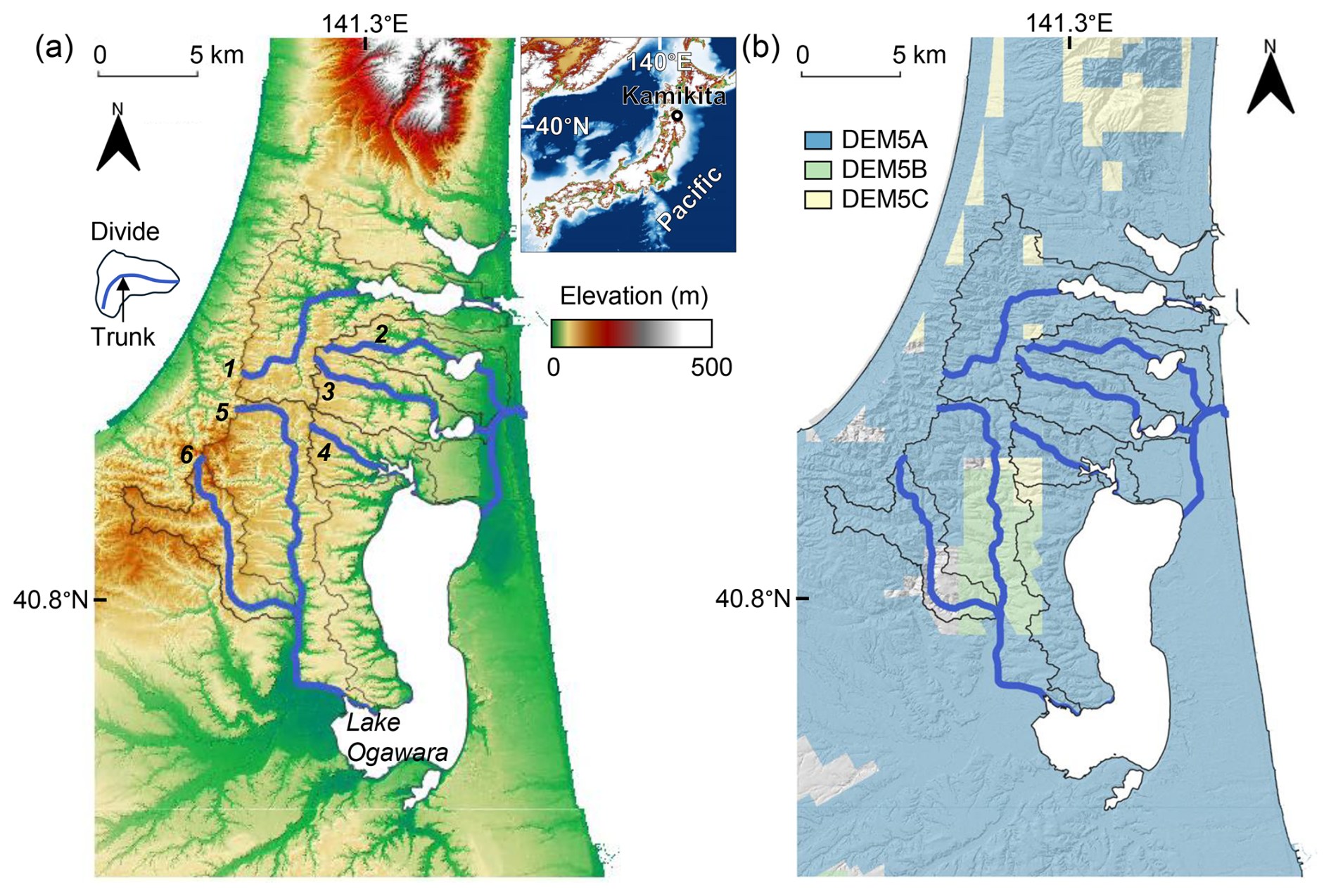
Figure 1 (a) Topography and (b) provided area of 5 m DEM by Geospatial Information Authority of Japan. For area where 5 m DEM is not provided, 10 m DEM was used.

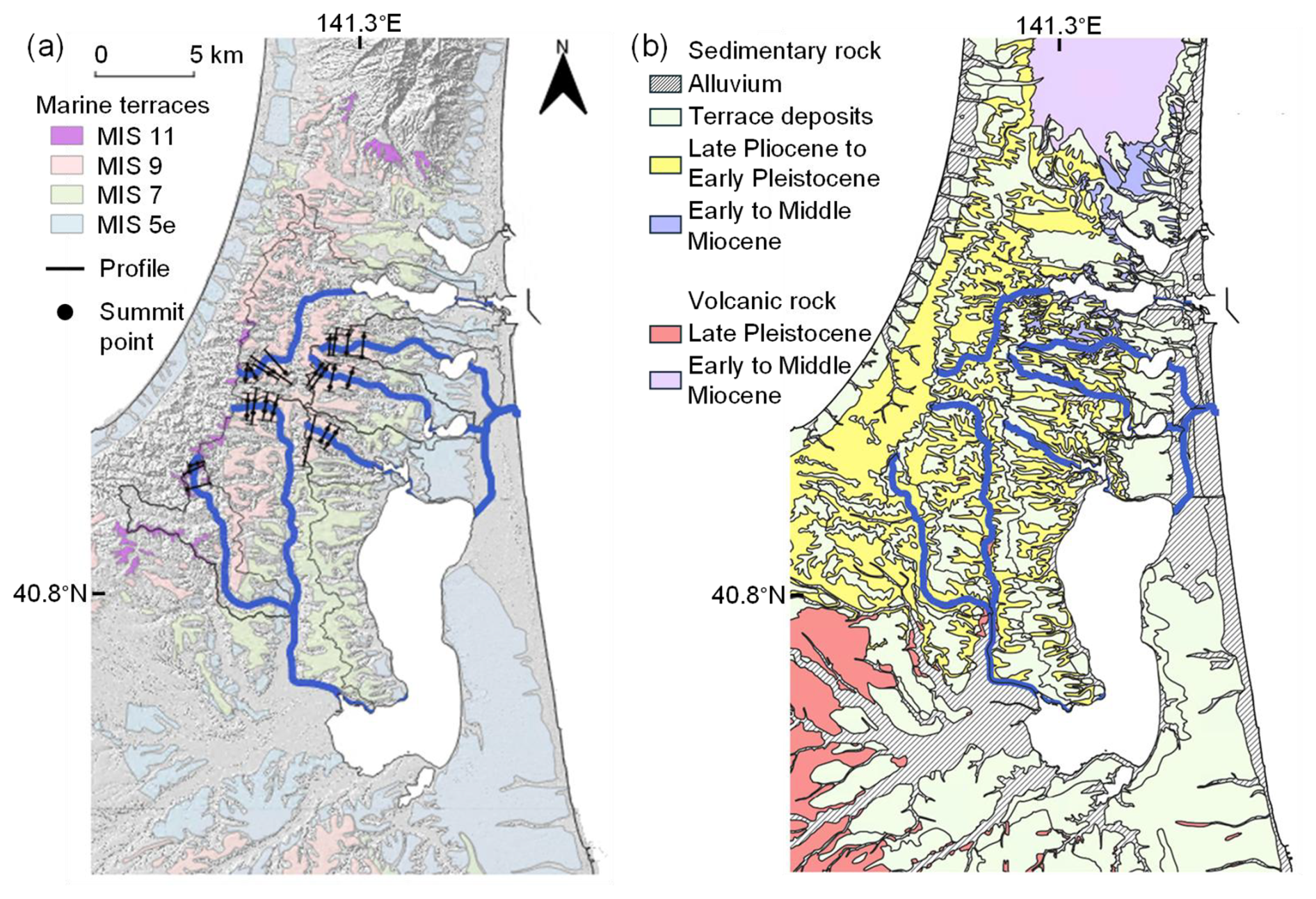
Figure 2 (a) Marine terraces and (b) geology of the study area. Marine terraces are based on Koike and Machida (2001). Geological map is based on the 1 : 200 000 scale geologic map (AIST, 2025). The summit levels extracted from profiles of the marine terrace surfaces were used for erosion rate estimates. Geological units are based on Kudo (2020).

Geological units of the Kamikita Plain are summarised by Kudo et al. (2020) (Fig. 2b). Bedrock was formed in the early to middle Miocene: the Takahoko Formation, sedimentary rock (16.6–13.1 Ma), which is mainly composed of pumice tuff, sandstone, and mudstone (Inohara et al., 2008), and the Tomari Formation, volcanic rock (16.6–15 Ma), characterized by basaltic to andesitic lavas and pyroclastic rocks (Kudo et al., 2020). Sedimentary rock units of late Pliocene to early Pleistocene, the Hamada Formation and the Katchi Formation, which primarily consist of sandstone and siltstone (Nemoto and Ujiie, 2009), overlay the bedrock. These sedimentary rocks are covered by terrace deposits of middle to late Pleistocene and alluvium. The mean annual rainfall in this region is around 1300 mm (JMA, 2026).

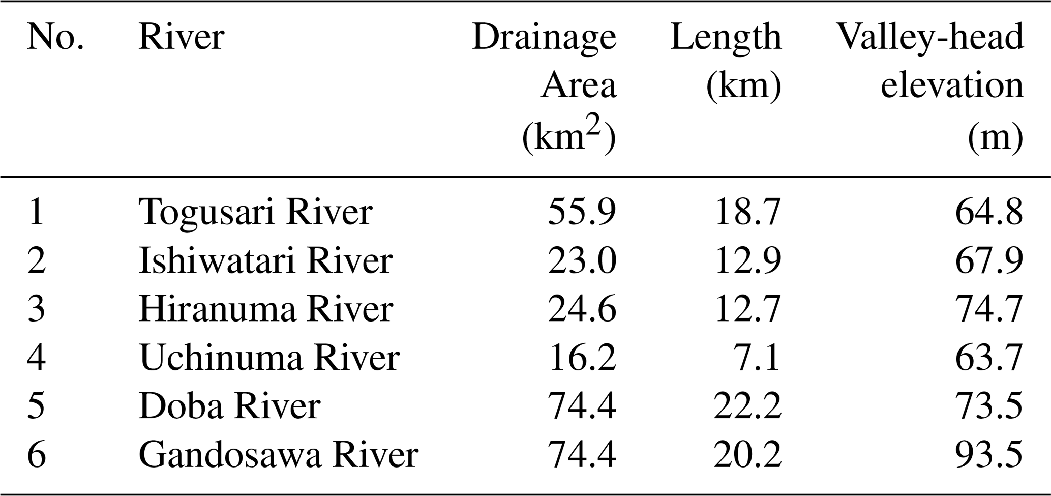
The Continental Divide is located in the western part of the study area. The valleys are deep on the west side of the divide and shallow on the east side. The rivers on the east side dissect the marine terraces and flow into the Pacific Ocean. Downstream the rivers, coastal lagoons such as Lake Ogawara are located, which were formed by sea-level fall during the Last Glacial Maximum and by subsequent development of sandbanks during the post-glacial period. In this study, we examined six streams flowing into the Pacific Ocean (1: the Togusari River, 2: the Ishiwatari River, 3: the Hiranuma River, 4: the Uchinuma River, 5: the Doba River, 6: the Gandosawa River) (Table 1), whose lithologic (sedimentary rock of Miocene to Pleistocene) and tectonic conditions (uplift rate ∼ 0.2 mm yr⁻¹) can be assumed to be uniform. Note that the rivers No. 2–6 are tributaries of the Takase River, which has a drainage area of 867 km² (MLIT, 2006) and flows from the Hakkoda Mountains located west of the study area. Volcanic rocks are distributed throughout the region and the tectonics differ from that of the Kamikita Plain; therefore, the Takase River was excluded from the scope of this study.

Table 1 Target rivers. Drainage area and length include coastal lagoons.

3 Methods

As previous research has shown (e.g., Whipple and Tucker, 2002; Whipple, 2004), most bedrock channels are mixed bedrock-alluvial channels partially covered by alluvium. In this case, the river profile consists of colluvial, bedrock, and alluvial sections (Fig. 3a). Empirical evidence suggests that many river profiles across different geological settings follow a power-law relationship between S and A, known as Flint's law (Hack, 1957; Morisawa, 1962; Flint, 1974):

$$\begin{array}{}\text{(3)}& S=k_{\mathrm{s}}{A}^{-\mathit{\theta }},\end{array}$$

where k_s [L^2θ] is the steepness index. The detachment-limited stream power incision model (Eq. 1) also predicts a similar slope-area scaling. Under the assumptions that K is constant (e.g., spatially uniform lithology and climate) and E has been measured (e.g., Hilley et al., 2019), the parameters in Eq. (1) can be inferred from k_s ($=(E/K{)}^{(\mathrm{1}/n)}$) and θ ($=m/n$) estimated using Eq. (3), without measuring stream power directly.

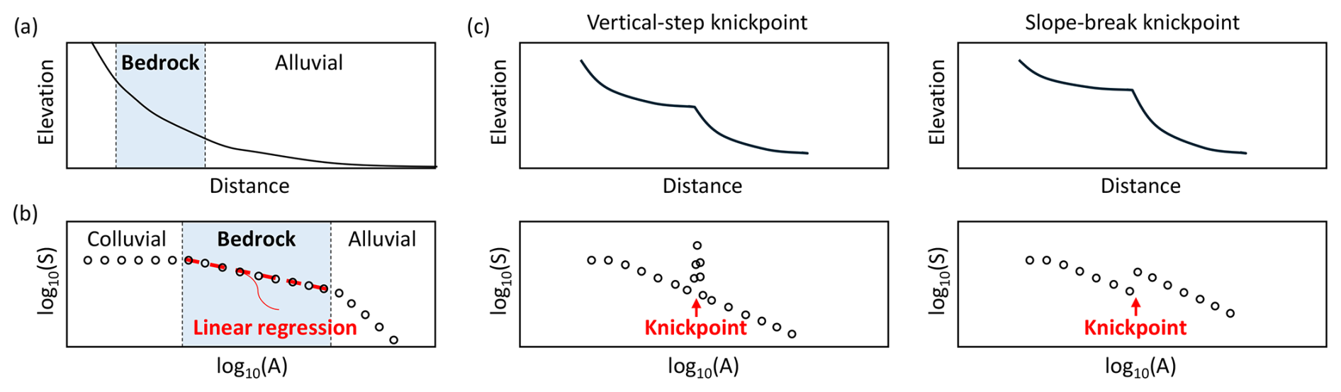
Figure 3 Schematic of (a) river profile, (b) slope-area plot, and (c) knickpoints (revised from Snyder et al., 2000, and Whipple et al., 2013).

Equation (3) implies that in detachment-limited reaches, the log-transformed slope-area plot can be fitted with a linear regression (Fig. 3b). Since channel transitions from bedrock to alluvial (i.e., DL to TL) or colluvial processes typically cause changes in channel slope (e.g., Whipple and Tucker, 1999, 2002; Stock et al., 2005), sections can be identified using the slope-area plot (Wang et al., 2017). Above a critical drainage area (A_c), colluvial processes, such as debris flows and land sliding, are dominant (Wobus et al., 2006). BelowA_c, the fluvial processes dominate. Both the bedrock and alluvial sections exhibit a descending gradient with increasing drainage areas (Whipple and Tucker, 2002). However, the transition to alluviated conditions causes a sudden reduction in channel gradient (Wobus et al., 2006).

Channels may contain knickpoints, which can be classified into two categories: vertical-step knickpoints and slope-break knickpoints (Fig. 3c). Vertical-step knickpoints correspond to sudden changes in elevation, such as waterfalls, and can be identified as spikes on the slope-area plot. These knickpoints are generally caused by channel-scale heterogeneities such as bounding faults (e.g., Kirby and Whipple, 2012; Liu et al., 2020).

Herein, we focused on slope-break knickpoints because they represent channel response to regional-scale perturbations, such as lithologic heterogeneity and sea-level fall (e.g., Haviv et al., 2010; Kirby and Whipple, 2012; Boulton, 2020). Unlike vertical-step knickpoints, these features mark a fundamental shift in the channel gradient, leading to abrupt changes in flow conditions. By identifying these slope-break knickpoints, we can evaluate how regional-scale factors influence river incision parameters.

This study estimated river incision parameters in three consecutive steps. First, sections exhibiting DL-like behaviours were identified from slope-area plots. Their validity was confirmed by comparing them with the alluvium distribution. We used a 5 m gridded digital elevation model (DEM), which is provided by the Geospatial Information Authority of Japan (Fig. 1b). Three types of 5 m DEM collected by different methods were combined: DEM5A (airborne LiDAR measurements), DEM5B and DEM5C (photogrammetry). There is also a 10 m DEM covering the entire country, which is created by interpolating topographic contour map with 10 m intervals. However, such a DEM can cause problems, such as artificial knickpoints due to interpolation errors or short-circuit meander bends in a river profile (Wobus et al., 2006). Therefore, we used the higher-resolution 5 m DEM. In areas where 5 m DEM is not available, such as the southeastern part of the Doba River and the middle of the Gandosawa River, 10 m DEM was bilinearly resampled to 5 m point spacing. Using the ArcHydrology toolbox (Tarboton et al., 1991), streams were extracted by applying a D8 flow routing algorithm and the trunk was defined from the Horton-Strahler number. To circumvent noise, previous research (Wobus et al., 2006; Whipple et al., 2007) has indicated that DEM-derived river profiles require the implication of some smoothing algorithms, such as a moving-window average. Furthermore, calculating the averaged channel slopes at a certain elevation interval or logarithmic bins of drainage area (log-bin averaging) was suggested (e.g., Snyder et al., 2000; Wobus et al., 2006). In previous studies utilizing the USGS 10 m DEM (root mean square error = 2.44 m; Gesch, 2007), Wobus et al. (2006) used moving-window sizes of 200 or 400 m, whereas Whipple et al. (2007) suggested an optimal window size of 250 m. The DEM datasets used herein possess a maximum measurement error (standard deviation) of 5 m, with specific accuracies ranging from 0.3 m (DEM5A), 0.7 m (DEM5B), 1.4 m (DEM5C), to 5 m (10 m DEM) (GIA, 2026). To ensure analytical consistency across the entire catchment and account for the largest measurement error, we smoothed elevation data using a 500 m moving window and calculated averaged slopes on 5 m contours and log-bin averaged slopes. We verified that no artificial knickpoints were generated at DEM tile boundaries.

In the second step, we calculated the channel concavity index from the integral approach within the detachment-limited reaches (Perron and Royden, 2013):

$$\begin{array}{}\text{(4)}& {\displaystyle }\mathit{\chi }=\underset{x_{\mathrm{b}}}{\overset{x}{\int }}{\left({\displaystyle \frac{A_{\mathrm{0}}}{A\left(x\right)}}\right)}^{\mathit{\theta }}\mathrm{d}x,\text{(5)}& {\displaystyle }z\left(x\right)=z\left(x_{\mathrm{b}}\right)+{\left({\displaystyle \frac{E}{K{A}_{\mathrm{0}}^m}}\right)}^{\mathrm{1}/n}\mathit{\chi }=z\left(x_{\mathrm{b}}\right)+\left({\displaystyle \frac{k_{\mathrm{s}}}{A_{\mathrm{0}}^{\mathit{\theta }}}}\right)\mathit{\chi },\end{array}$$

where x [L] is the horizontal upstream distance from an outlet; x_b [L] is the distance at the outlet (in this study, x_b = 0); and z [L] is elevation. The validity of the bedrock sections identified by slope-area plots is confirmed again by the linearity of χ plot. As shown in Eqs. (3) and (5), local k_sn values and their channel-averaged values can be calculated either from (1) the slope-area approach (e.g., Wobus et al., 2006; Scherler et al., 2014) or (2) the slope of χ plots (hereafter k_{sn_χ}: e.g., Perron and Royden, 2013; Gailleton et al., 2019). The slope-area approach preserves local signals associated with knickpoints, whereas k_{sn_χ} is comparatively smoother and less sensitive to noise (Gailleton et al., 2019). Previous studies have compared these two approaches (e.g., Scherler et al., 2014; Neely et al., 2017) and demonstrated that the choice of method should depend on the context and objective of a study. In this study, we primarily used local k_sn ($=S{A}^{{\mathit{\theta }}_{\mathrm{ref}}}$) and its channel-averaged values derived from the slope-area approach (e.g., Takahashi et al., 2022). This is because our objectives include investigation of the transient steepening and lithological signals associated with slope-break knickpoints, which may be partially smoothed in k_{sn_χ} despite its lower sensitivity to noise. For channel-averaged k_sn, k_{sn_χ} was additionally calculated to evaluate the robustness of the results.

Using a reference basin area of A₀ = 1 m², the concavity index (θ) and knickpoint locations were estimated using a statistical segment-fitting algorithm (Mudd et al., 2014). In this algorithm, the optimal θ is evaluated in χ space by minimizing the corrected Akaike Information Criterion (AICc) across all possible contiguous channel segments.

$$\begin{array}{}\text{(6)}& \mathrm{AICc}=\mathrm{AIC}+{\displaystyle \frac{\mathrm{2}k(k+\mathrm{1})}{N-k-\mathrm{1}}},\mathrm{AIC}=\mathrm{2}k+{\displaystyle \frac{RSS}{{\mathit{\sigma }}_z^{\mathrm{2}}}}\end{array}$$

where N is the number of channel nodes, s is the number of segments (k=2s), RSS is the residual sum of squares between data points and regression lines, and σ_z is the standard deviation of elevation measurements, including geomorphic noise. In this study, we used DEM5A (standard deviation: 0.3 m) in detachment-limited reaches, and σ_z was conservatively set to 0.6 m. A bootstrapping method was employed with 1000 independent trials to evaluate the robustness of the results. In this method, channel nodes were randomly skipped using a uniform distribution ranging from 0 to 2×n_sk. Following Gailleton et al. (2019), n_sk was set to 1. θ_ref was determined using a collinearity test that minimized the sum of AICc values across all analyzed rivers. Because χ profiles were segmented into channel reaches of unequal length, channel-averaged k_{sn_χ} was calculated as the stream-length-weighted mean of segment slopes to avoid overrepresentation of short reaches. Knickpoints were defined as boundaries between adjacent segments. Knickpoint type was classified using the slope ratio of regression lines (S_ratio) and elevation difference (Z_jump) across these boundaries: large Z_jump with a minimal change in S_ratio indicates a vertical-step knickpoint, whereas a significant change in S_ratio with negligible Z_jump indicates a slope-break knickpoint. In accordance with Gailleton et al. (2019), knickpoints were extracted using the optimal θ specific to each river. To remove minor knickpoints, we applied thresholds of Z_jump = 5.0 m and S_ratio = 0.2. These values are broadly consistent with those used in previous studies: Neely et al. (2017) applied a minimum knickzone height of 5 m for 10 m DEM, and Gailleton et al. (2019) used a threshold of $\left|\mathrm{\Delta }{k}_{\mathrm{s}n}\right|$ (the difference in slope of regression lines) = 0.8 for k_sn values ranging from 0.5 to 5.0.

In the third step, the values of n and K were estimated. Within the detachment-limited reaches, the relationship between E and k_sn is expressed as:

$$\begin{array}{}\text{(7)}& E=K{k}_{\mathrm{s}n}^n.\end{array}$$

Taking the natural logarithm of Eq. (7) allows n and K to be estimated via the regression analysis of E and k_sn (e.g., Leonard et al., 2023):

$$\begin{array}{}\text{(8)}& \ln \left(E\right)=n\ln \left(k_{\mathrm{s}n}\right)+\ln \left(K\right),\end{array}$$

where n and ln (K) represent the slope of the regression line and the intercept, respectively. River terraces are not identified in the study area (Koike and Machida, 2001). Since the target rivers incising marine terraces have smooth and concave-up profiles, long-term incision rate E was approximately calculated based on the height of marine terraces:

$$\begin{array}{}\text{(9)}& E=\left(z_{\mathrm{t}}-z_{\mathrm{r}}-d\right)/T_{\mathrm{t}},\end{array}$$

where z_t [L] is the summit level of the marine terrace; z_r [L] is the present river profile; d [L] is the thickness of tephra and loess; and T_t [T] is the formation age of the river. The summit level of the marine terrace was reconstructed by interpolating the highest elevations from multiple topographic profiles extracted from preserved marine terrace surfaces (Fig. 2a; see Figs. S1–S6 in the Supplement for detailed maps and profiles). Where summit levels were comparable on both banks of the river, their average value was used. T_t was approximated as the terrace age where valley head is located.

Table 2 Probability distribution used for uncertainty analysis of erosion rate.

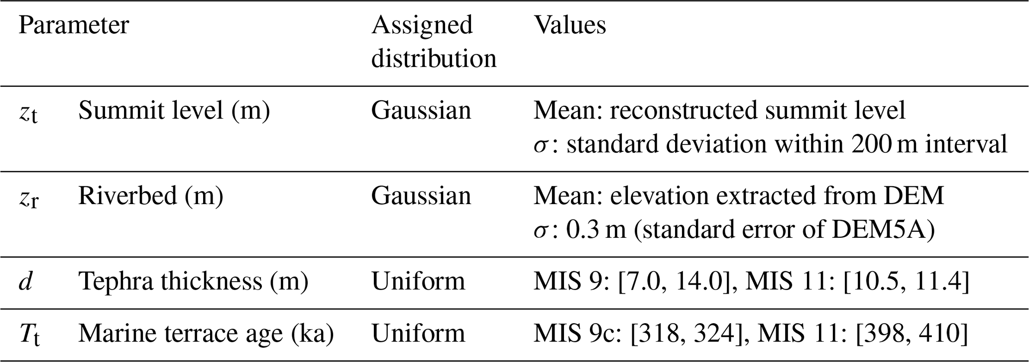
To ensure spatial consistency, E and k_sn were compared at equal intervals of 200 m along the river channels, following the approach for parameter estimation using strath terraces by Lague (2014). To account for uncertainties in E (Eq. 9), a Monte Carlo simulation with 100 000 iterations was performed based on the inherent probability distribution of all input parameters (Table 2). Elevation uncertainty was modeled as a Gaussian distribution based on DEM precision (0.3 m for DEM5A) in the detachment-limited reaches. The uncertainties in terrace age (T_t) and tephra thickness (d) were represented using uniform distributions derived from field observations.

T_t values were adapted from those reported by Matsu'ura et al. (2019) for the Kamikita Coastal Plain: 398 to 410 ka (MIS 11), 318 to 324 ka (MIS 9c), 230 to 235 ka (MIS 7e), 212 to 220 ka (MIS 7c), and 116 to 132 ka (MIS 5e). Furthermore, d values were derived from observed data of tephra layers and loam (tephric loess) in the study area. The main tephra layers are as follows (Kudo, 2023): Hakkoda second-stage (Hkd2: 0.19–0.29 Ma) and White Pumice (WP: 210 ka) erupted from the Hakkoda Volcano; Orange Pumice (OrP: 166 ka) and Towada-Ofudo (To-Of: 36 ka) erupted from the Towada Volcano; and Toya (106 ka) erupted from the Toya Volcano. Based on outcrop observations at seven locations, AIST (2015, 2016) has identified the tephra and loam thickness as 11.4 m (sampled at Onadesawa) and 10.5 m at Kanaya for MIS 11; 14 m at Shichihyaku and 7 m at Kamiyoshita for MIS 9; 6 m at Hotozawa for MIS 7; 2 m or 4 m at Neinuma for MIS 5e (the outcrop locations: Fig. S7). For the MIS 5e marine terraces, Koike and Machida (2001) indicated that the thickness of cover deposit layers is 2 m at four points to 3 m at one point. Note that Kudo (2023) provides an approximate estimate of the spatial distribution of tephra thickness for the Towada Volcano. However, this information is not provided for other volcanoes. Accordingly, a uniform thickness was assigned to each terrace stage (Table 2). This Monte Carlo approach enables the evaluation of the parameter reliability by accounting for uncertainties in summit level, riverbed elevation, tephra thickness, and marine terrace age.

4 Results

4.1 Channel profiles

Longitudinal river profiles, slope-area plots, and χ plots for six rivers are shown in Fig. 4. A_cr is confirmed at ∼ 0.1 km² for all rivers, which is consistent with earlier studies (e.g., Montgomery and Foufoula-Georgiou, 1993; Stock and Dietrich, 2003; Wobus et al., 2006). In the slope-area plots (Fig. 4b), all rivers exhibit an approximately linear descending gradient with increasing drainage areas. The gradients suddenly reduce around A = 1–10 km² upstream of the alluvium distribution. This is consistent with previous research on mixed bedrock and alluvial channels (Snyder et al., 2000; Wobus et al., 2006, Wang et al., 2017), reflecting a transition to alluviated conditions due to the sea level rise during the Holocene. Therefore, the studied rivers are considered to be mixed bedrock and alluvial channels, and the sudden decrease in the channel gradient corresponds to the transition from erosive bedrock channels (DL) to depositional alluvial channels (TL).

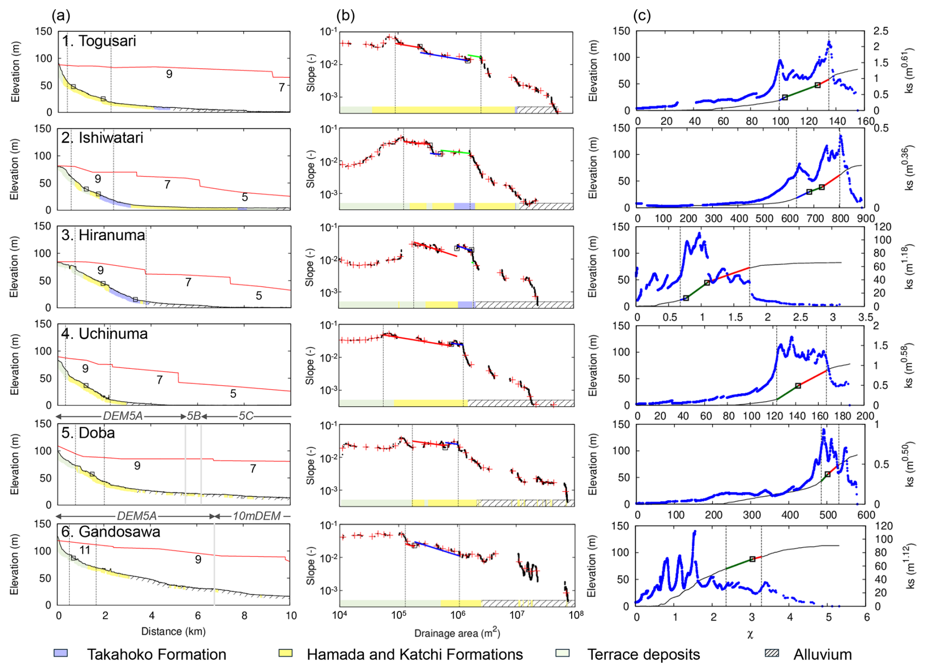
Figure 4 Stream profile analysis of the study area. (a) Longitudinal profile (black line) and the elevation of marine terraces (red line) with Marine Isotope Stages. Squares denote knickpoints. Gray lines for rivers No. 5 and 6 indicate the boundaries of DEMs other than DEM5A (LiDAR 5 m DEM). (b) Slope-area plot. Average channel slopes are calculated on 5 m contours (black point) and by the log-bin averaging method (red mark). (c) χ plot (black line) with k_s (blue point) based on the concavity of each river. In all graphs, dashed lines and color bold lines (red, blue, and green) correspond to the bedrock section and its regression line.

Table 3 Formation ages and concavity indices (with standard deviation).

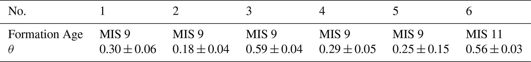
The θ values estimated for detachment-limited reaches are summarised in Table 3 and Fig. 5. The optimal θ values for each river range from 0.18 to 0.59 (Fig. S8 shows the AICc values). Meanwhile, θ_ref was estimated to be 0.44 ± 0.10 (standard deviation) using the collinearity test (Fig. 5b), which lies within the general range of steady-state channels (θ = 0.35–0.6: Kirby and Whipple, 2012) and closely aligns with the typical reference concavity of 0.45 (e.g., Wobus et al., 2006). Snyder et al. (2003) indicates that even considering sea-level changes, a quasi-steady-state condition has been achieved in the upper parts of the channel. Therefore, although the target rivers tend to fluctuate from their mouths to their divides reflecting sea-level change, it can be assumed that they have approached the quasi-steady state in the upstream section. However, as θ_ref can impact the estimation of river incision parameters, we evaluated k_sn using θ_ref values of 0.4, 0.5, and 0.6 to ensure robustness.

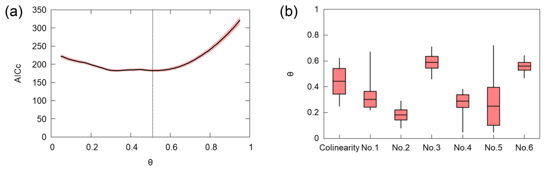
Figure 5 (a) AICc values for the regional collinearity test and (b) the distribution of optimal θ for regional and individual river basins. In panel (a), the solid line and shaded red area indicate the mean and ±1σ (standard deviation) interval for 1000 bootstrap trials. In panel (b), the whiskers indicate the range between minimum and maximum values, while the boxes represent the mean and ±1σ interval.

Table 4 and Fig. 6 show the extracted knickpoints and their locations on the map (Fig. 4c). All knickpoints are classified as slope-break knickpoints and do not correspond to the boundaries between different DEM datasets. Except for the second knickpoint of river No. 2, the knickpoints are not located near lithological boundaries. Instead, they are distributed at similar elevations (around E.L. 25 and 50 m). This suggests that they can be base-level-fall related upstream-migrating knickpoints. In the Sanriku Coast, approximately 50 km south of the study area, Ogami (2015) indentified upstream-migrating knickpoints in multiple rivers which were formed during the sea-level highstands during MIS 5e, 7, 9, and 11. The knickpoints in the study area may have been formed for the same reason. Note that in river No. 6, which formed earlier than the other rivers (MIS11), a knickpoint is observed at a higher elevation of 88 m. This knickpoint could have been formed during a preceding sea-level cycle.

Table 4 Extracted knickpoints.

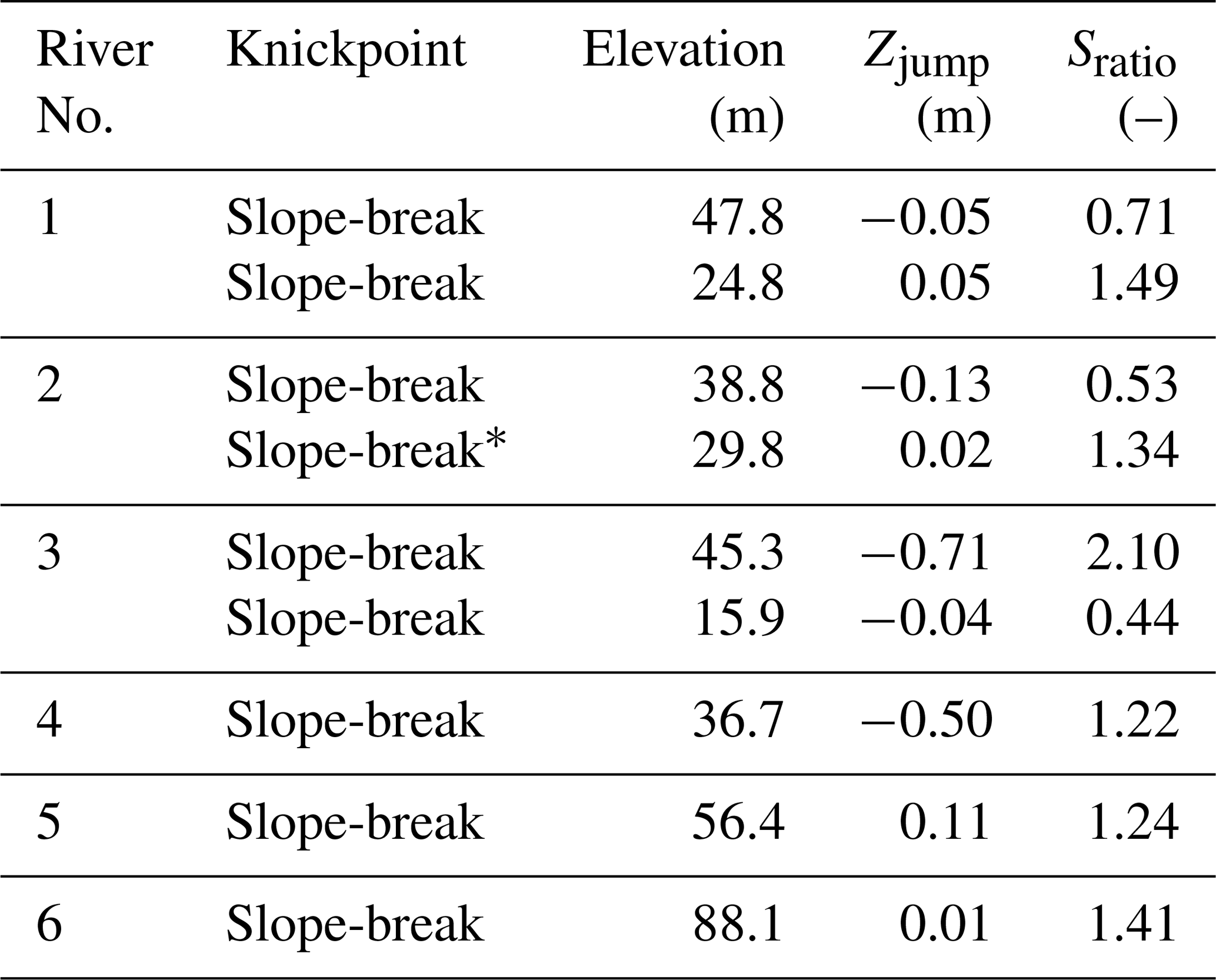
^∗ This knickpoint is located approximately 50 m upstream from the lithological boundary (Hamada/Katchi and Takahoko Formations) along the river channel.

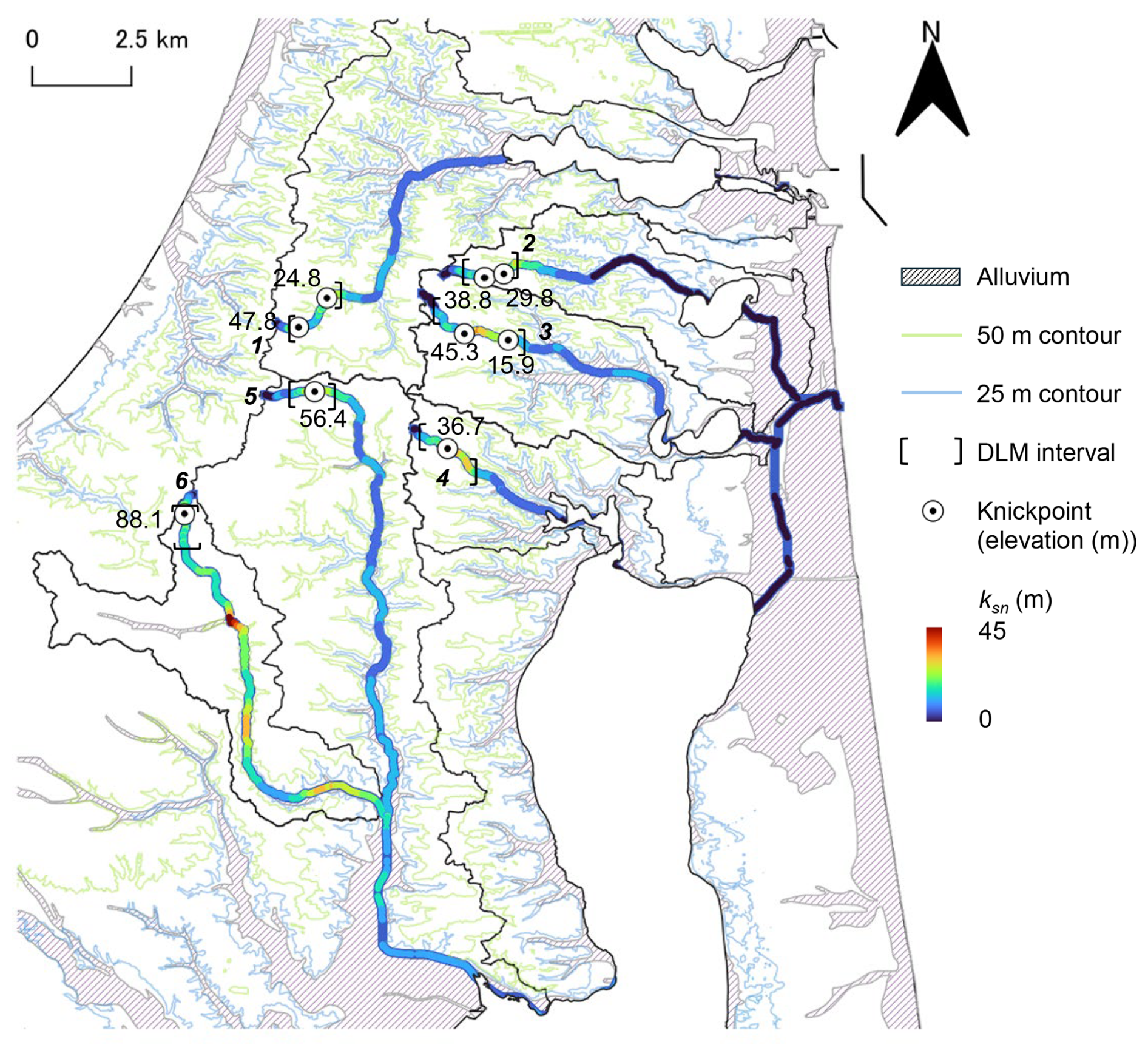
Figure 6 Knickpoints (points with elevation (m)) and 25 and 50 m contours (blue and green lines) within the detachment-limited reaches. Color along the rivers demonstrates k_sn (θ_ref = 0.5).

The second knickpoint of river No. 2 is located near the boundary between the Hamada and Katchi Formations and the Takahoko Formation (Fig. 4a). As discussed in Sect. 5.2, the Takahoko Formation exhibits higher N-values (80–137) compared with the Hamada and Katchi Formations (50–63). This contrast in rock hardness likely contributed to the formation of this lithological knickpoint. The same boundary is also located near the first knickpoint of river No. 3; however, because its elevation is close to 50 m, this knickpoint might be affected by both the lithological difference and sea-level changes.

4.2 River incision parameters

E and k_sn were compared at 200 m intervals along the river channels (Fig. 7a–c). A positive correlation between E and k_sn was observed across all θ_ref values. The correlation coefficient (R) increased with increasing θ_ref, ranging from 0.37 to 0.59. Across the range of θ_ref = 0.4–0.6, the estimated n values consistently indicated a nonlinear relationship (n > 1) and fell within a narrow range from 1.14 to 1.34. In contrast, the estimated K varied over a considerably wider range from 4.2 × 10⁻⁷ to 1.3 × 10⁻⁵. The 90 % confidence intervals for these parameters were n = [0.94, 1.28], [1.15, 1.46], and [1.10, 1.36], and K = [1.0 × 10⁻⁶, 2.9 × 10⁻⁶], [1.1 × 10⁻⁶, 2.9 × 10⁻⁶] and [2.5 × 10⁻⁷, 7.8 × 10⁻⁷] for θ_ref = 0.4, 0.5 and 0.6, respectively (Fig. 8 shows the results obtained at θ_ref = 0.5).

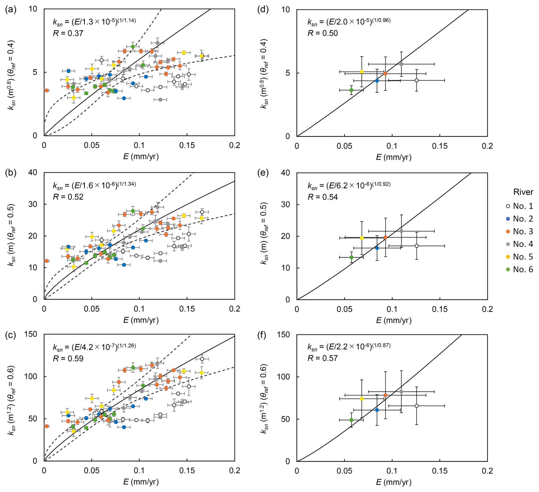
Figure 7 River incision rate versus channel steepness index k_sn within the detachment-limited reaches: (a–c) sampled at 200 m intervals and (d–f) averaged for each reach, both for θ_ref = 0.4, 0.5, and 0.6. Error bars denote ±1σ. The bold and dashed lines indicate the regression lines and their 90 % confidence intervals.

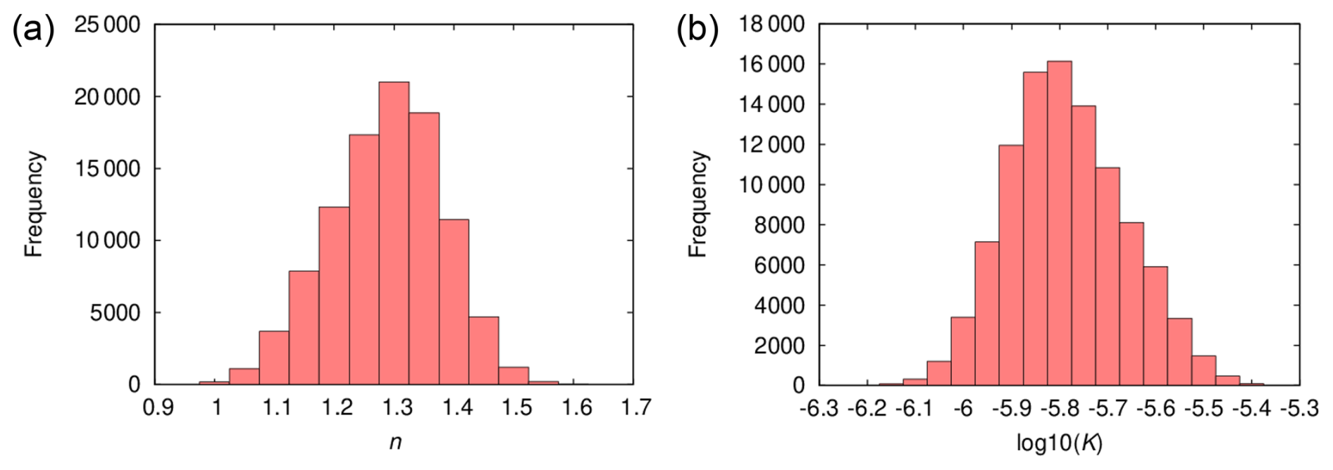
Figure 8 Probability distributions of n and K values estimated from 100 000 Monte Carlo simulations (θ_ref = 0.5).

Table 5 River incision parameters (n and K) and correlation coefficient estimated for each river (θ_ref = 0.5).

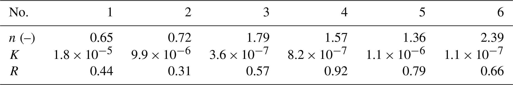
Table 5 shows the parameter values obtained for each river. Although a relatively high correlation could be confirmed for rivers Nos. 3–6 (R≥0.65), values of K vary by nearly one order of magnitude. Similarly, the values of n exhibited inter-river variability; n > 1 for rivers Nos. 3–6, whereas n < 1 for rivers Nos. 1 and 2.

5 Discussions

5.1 The value of n

In Sect. 4.2, the estimated values of n (1.14 to 1.34) indicate a nonlinear relationship (n > 1) between E and k_sn across θ_ref of 0.4–0.6. Specifically, for θ_ref = 0.5 and 0.6 where R≥0.5, the 90 % confidence interval for n lie entirely above 1.1. This nonlinear relationship is consistent with previous research conducted in various regions, where most estimates of n are between 1 and 2 (e.g., Ouimet et al., 2009; DiBiase et al., 2010; Lague, 2014; Harel et al., 2016; Campforts et al., 2020; Gallen and Fernandez-Blanco, 2021; Leonard et al., 2023). In addition, slope-break knickpoints occurred at similar elevations across multiple rivers, which do not correspond to boundaries of lithology or different DEM datasets.

Meanwhile, when we compared the averaged E and k_sn values within detachment-limited reaches, n was approximately 1 across all θ_ref values (n = 0.96, 0.92, and 0.87 for θ_ref = 0.4, 0.5, and 0.6; Fig. 7d–f). Furthermore, when river No. 1 was excluded and only tributaries within the same drainage area (the Takase River) were compared, n was 1.05 with a higher R of 0.79.

To evaluate the robustness of our results, we additionally compared the averaged E and k_{sn_χ}. Similar to previous studies (e.g., Scherler et al., 2014; Neely et al., 2017), channel-averaged local k_sn and k_{sn_χ} showed strong correlations (R² = 0.98–0.99; Fig. S9a–c). Compared with channel-averaged local k_sn, the use of k_{sn_χ} yielded slightly smaller n values (0.75–0.83; Fig. S9d–f). This result is consistent with Scherler et al. (2014) and likely reflects the comparatively smoother nature of k_{sn_χ}, which reduces the influence of localized transient steepening associated with slope-break knickpoints. Nevertheless, the overall trends remained unchanged regardless of the choice of k_sn: (1) the nonlinear relationship observed for local k_sn (n > 1) weakened toward n ∼ 1 when channel-averaged k_sn was used, and (2) excluding river No.1 improved the correlation among tributaries within the Takase River basin.

These results suggest that the observed nonlinearity is likely an apparent effect caused by the presence of migrating knickpoints triggered by sea-level change (Pavano, 2025), rather than reflecting the intrinsic physics of river incision processes. Although most rivers yield n > 1, river Nos. 1 or 2 exhibited n < 1. For river No. 1, n < 1 possibly reflects the differences in watershed and downstream boundary conditions. Unlike other tributaries that flow into the large Lake Ogawara within the Takase River basin (867 km²), river No. 1 has a small drainage area (55.9 km²) and flows into the small Takahoko pond. These contrasting base-level conditions can lead to different transient response at the catchment scale, causing fluctuations in n values. For river No. 2, the presence of a lithological boundary, where the downstream lithology is more erodible than upstream lithology, may result in a lower n value.

Nevertheless, the intrinsic physics of river incision processes may also contribute to the observed nonlinearity. Such physical factors include shear stress thresholds, plucking, channel-width effects, and sediment-flux-dependent incision processes such as abrasion, tool effects, and cover effects (Whipple et al., 2000; Gasparini and Brandon, 2011; Yamanishi and Naruse, 2026). The main target lithology comprises soft sedimentary rocks (q_u≤3 MPa, as discussed in Sect. 5.2), where the tool and cover effects of riverbed gravel are likely minimal due to rapid disintegration into fine sediments; however, two possibilities remain: shear stress threshold and abrasion. In the small-scale catchments, the base flow discharge may be insufficient to exceed the critical shear stress required for bedrock incision. In addition, the abundance of sand derived from soft bedrock may cause suspended-load abrasion, which theoretically supports n values of ∼ $\mathrm{5}/\mathrm{3}$ (Whipple et al., 2000). Note that the neglected effect of channel width is limited, since parameter estimation was performed in the limited upstream and midstream areas (Fig. 6). While the relative contributions of these transient responses and physical processes require further comprehensive investigation, the estimated parameters represent robust time-averaged behavior integrated over multi glacial–interglacial cycles.

5.2 The value of K

The value of K can vary by orders of magnitude due to lithology, climate, tectonics, hydraulic processes, and other environmental conditions (e.g., Murphy et al., 2016; DiBiase et al., 2018; Chen et al., 2019; Seybold et al., 2021). Among them, Haag and Schoenbohm (2025) confirmed a strong correlation (R² = 0.89) between global estimates for K based on ¹⁰Be erosion rates (Harel et al., 2016) and Schmidt hammer-derived lithologic erodibility (K∝L_E, $L_{\mathrm{E}}=q_{\mathrm{u}}^{-\mathrm{2}}$; Sklar and Dietrich, 2001; Turowski et al., 2023); where L_E is the lithologic erodibility (Campforts et al., 2020) and q_u is unconfined compressive strength (Fig. 9).

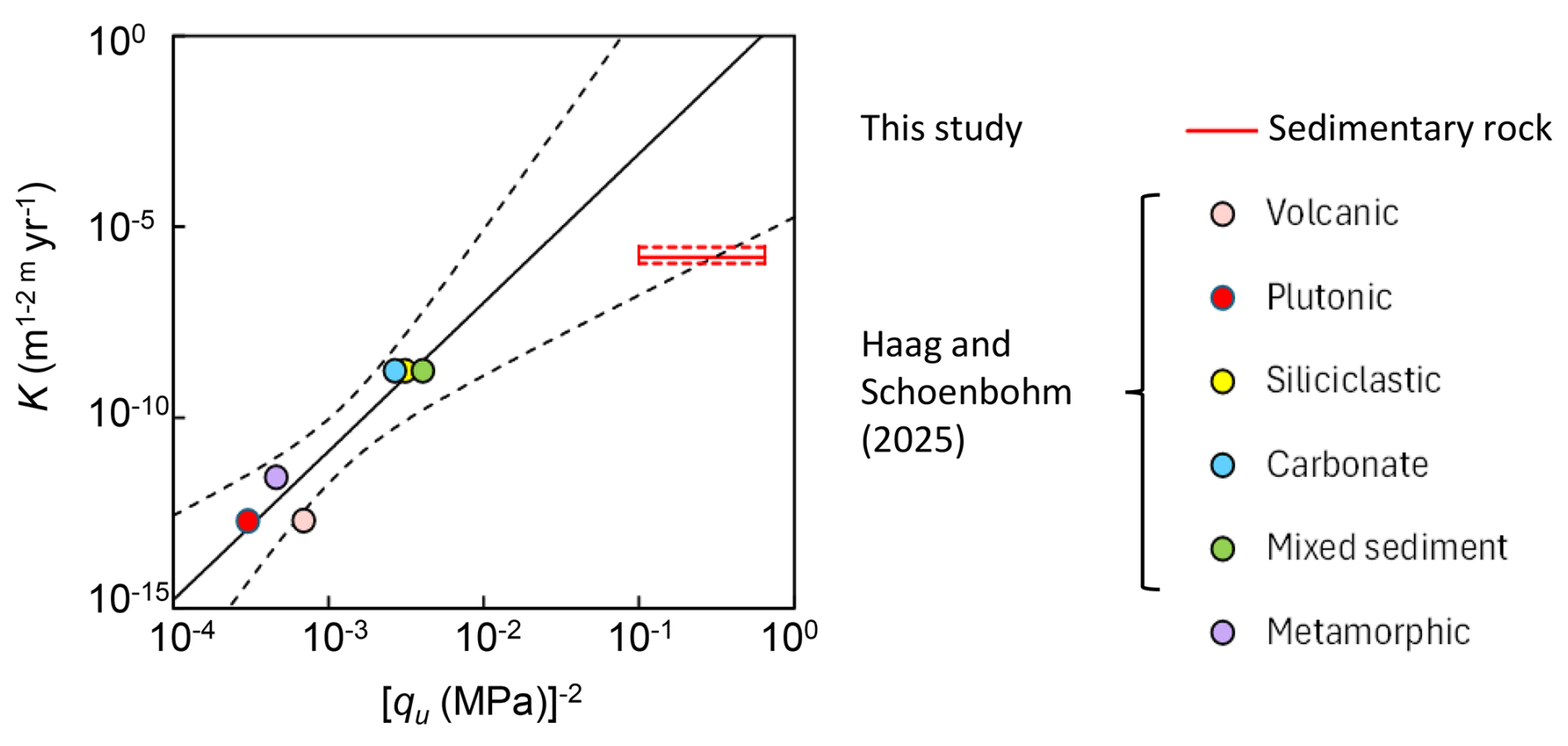
Figure 9 Comparison between the results of this study and data of Haag and Schoenbohm (2025) (color points) for unconfined compressive strength q_u and erosional coefficient K. The box plot shows the best estimate and 90 % confidence interval of our results based on the log-bin averaged data for all the rivers. The black line and dashed lines are the best estimate and 90 % confidence interval shown in Haag and Schoenbohm (2025).

In this section, estimates for K for this study and the relationship between K and q_u in Haag and Schoenbohm (2025) were compared at the same θ_ref of 0.5. In the study area, measured N-values from previous studies for each lithology are as follows (Onuma, 1972; Planning Bureau, Ministry of Construction, Japan, 1997): 25–41 for the terrace deposits, 50–63 for the Hamada and Katchi formations, and 80–137 for the Takahoko formation. We then converted the N-values to q_u (q_u = 25–50 N MPa: Japanese Geotechnical Society, 2015): 0.6–2.0 MPa for the terrace deposits, 1.2–3.1 MPa for the Hamada and Katchi formations, and 2.0–6.8 MPa for the Takahoko formation. For the Hamada and Katchi formations of which the studied rivers mainly consist, estimated values are almost within the 90 % confidence interval of the regression line of Haag and Schoenbohm (2025) (Fig. 9). In Sect. 4.2, the estimated K value was 1.6 × 10⁻⁶ [1.1 × 10⁻⁶, 2.9 × 10⁻⁶]. Although rock strength in this study is out of range of the previous study (q_u = 10–100 MPa), a strong correlation was observed between the results of this study and the data in Haag and Schoenbohm (2025) with R² = 0.84. This highlights the significant influence of bedrock lithology on K, as indicated by previous research (e.g., Campforts et al., 2020; Haag and Schoenbohm, 2025).

However, the results of this study underestimate K (the regression line) in the work of Haag and Schoenbohm (2025). This discrepancy is likely caused by three potential reasons. First, as discussed in Sect. 5.1, the influence of sea-level changes may lead to an underestimation of K. When comparing the average k_sn and E in the river section, which effectively smooths the transient knickpoint migration due to sea-level changes, the estimated K value increased to 6.2 × 10⁻⁶ [7.7 × 10⁻⁸, 5.1 × 10⁻⁴], approaching the relationship described by Haag and Schoenbohm (2025) (Fig. 9). Note that the estimated K value using k_{sn_χ} remains within the same order of magnitude as that estimated using channel-averaged local k_sn, differing by less than a factor of two (Fig. S9d–f).

Second, the discrepancy may arise from the use of present values of k_sn to compare with long-term average erosion rates. Since the target rivers have been formed gradually by incising the flat marine terraces, long-term average k_sn should be less than the present value. If the long-term average k_sn is half of present k_sn, the estimated K doubles without changing the n value.

Third, the cohesion of the main riverbed lithologies (the Hamada and Katchi Formations), which are semi-consolidated sedimentary rocks with q_u = 1.2–3.1 MPa that primarily consist of sandstone and siltstone (see Sect. 2), may function as a resistive factor. This cohesion increases the shear stress threshold and leads to the dissipation of stream power. Since standard mechanical indicators such as N-values often fail to fully capture the cohesive resistance inherent in these semi-consolidated units, the resulting K values may fall near the lower bound of the global relationship.

6 Conclusions

This study estimated the river incision parameters for soft sedimentary rock, which are lacking in previous global compilations. The study targeted the Kamikita Coastal Plain, where bedrock lithology (sedimentary rocks of Miocene to Pleistocene) and uplift rate (approximately 0.2 mm yr⁻¹ over the past 300 ka) are assumed to be uniform. Parameter values were estimated using slope-area analysis based on river incision rates approximately derived from marine terraces (MIS 5e, 7, 9, and 11) widely distributed in the area. A summary of the main results is as follows.

DL-like behaviour was confirmed in the limited upstream and midstream area (A ≥ 10⁵ m²) located upstream of the alluvium distribution for all rivers. Although the optimal θ value varied from 0.18 to 0.59 for each river, θ_ref was estimated to be 0.44 ± 0.10, which falls within the typical range for steady-state channels (0.35–0.6).

Across the θ_ref range of 0.4 to 0.6, exponent n consistently exhibited a nonlinear relationship, ranging between 1.14 and 1.34, which aligns with the previous global compilation of 1 to 2. This nonlinearity can be due to past sea-level changes, causing slope-break knickpoints at similar elevations.

For target rivers consisting mainly of late Pliocene and early Pleistocene sedimentary rock, erosion coefficient K was estimated to be 10⁻⁵–10⁻⁶ m^0.1 yr⁻¹. Estimated K is almost within 90 % confidence interval of the previous global relationship with unconfined compressive strength q_u ($K\propto \mathrm{1}/q_{\mathrm{u}}^{\mathrm{2}}$). This supports the significance of bedrock lithology on K, as previously reported (e.g., Campforts et al., 2020; Haag and Schoenbohm, 2025).

These results represent long-term average erosion trends integrated over multiple glacial–interglacial cycles (since MIS 9 or 11). Consequently, the estimated n and K values are considered to reflect integrated values that account for past temporal variations in external forcing, such as climate and sea-level changes. For long-term safety assessments, such as those required for radioactive waste disposal, these parameters serve as a basis for time-dependent simulations of future landscape evolution over a glacial–interglacial cycle (∼ 10⁴ to 10⁵ years). Such simulations can be implemented using mixed DL and TL models, incorporating these time-varying external forcing and additional geomorphic processes, such as hillslope and coastal sediment transport (e.g., Salles et al., 2018). Using the estimated n and K values as the baseline, this approach could enable the reliable prediction of not only the maximum erosion depth, but also the spatial distribution of erosion across the site and its subsequent effects on groundwater flow systems. To further verify the estimated parameters, our next step will be the reproduction of past landscape evolution by numerical landscape evolution models using mixed DL and TL models.