Discrete differential geometry of fluvial landscapes

Geomorphology as a discipline is defined by the use of topographic form to understand surface processes on Earth and other planets. In practice this requires drawing connections between quantitative metrics of surface geometry and rates of erosion and deformation, to understand the spatial partitioning of different erosion processes and the feedback between them. Curvature, perhaps the most fundamental way to measure and categorize surfaces of any kind, also appears explicitly in many erosion models and is therefore of significance to geomorphology. However, there is ambiguity in how curvature of discretely sampled topographic surfaces such as digital elevation models is defined and calculated. In this study we use a formal surface theory approach to compute intrinsic and extrinsic curvature metrics, and associated shape-class distributions, of approximate steady-state fluvial topography of the Oregon Coast Range, USA. We develop a workflow, including careful spectral filtering to isolate wavelengths of interest, that provides a nuanced view of landscape geometry that is consistent and accurate across steep landscape regions. Two invariants of the curvature tensor – the mean and Gaussian curvatures – reveal systematic structure of topographic geometry in channel and ridge networks that captures transitions between hillslope, debris flow, and fluvial process regimes. Mean curvature and associated shape classes are equipartitioned between concave-down and concave-up elements, forming complementary branching structures that span the landscape. These results suggest that formal surface theory approaches could prove valuable in improving process regime identification from digital elevation data in fluvial landscapes.

1 Introduction

The Earth's surface contains multi-scale signatures of the processes that have shaped it. Over length scales of 10²–10⁴ km, long-wavelength relief tracks patterns of lithospheric deformation and isostasy (Wieczorek, 2015) with relief generally increasing with the horizontal scale of measurement (Turcotte, 1987). The resulting gravitational gradients drive surface erosion that shapes the landscape at finer scales (Perron et al., 2008; Hooshyar et al., 2020; Bonetti et al., 2020) through a combination of diffusive (Fernandes and Dietrich, 1997), advective (Whipple and Tucker, 1999), and stochastic mass transport (Furbish et al., 2009).

In the spirit of reductionism, geomorphic studies often focus on regions where a single erosion process is assumed dominant. There are many established approaches to partitioning the landscape into process domains (Montgomery and Foufoula‐Georgiou, 1993; Shary, 1995; Jasiewicz and Stepinski, 2013). However, compartmentalization comes at the risk of oversimplifying interactions between processes. For example, the transition from hillslopes to fluvial channels commonly occurs in topographic hollows where gullies begin to incise. Here, interactions between hillslope and fluvial processes influence both long-term landscape evolution (Reneau and Dietrich, 1991) and short-term mass motions that are of interest for hazard prediction (Yanites et al., 2025). As another example, the transition from curved hilltops to linear hillslopes spans a geometric transition that requires accurate quantification of both slope and curvature with changing surface orientation (Roering et al., 1999). As digital elevation models (DEMs) become increasingly high resolution in space and multitemporal (Crosby et al., 2020), there are growing opportunities to understand landscapes holistically using quantitative tools that are accurate and informative across all regions of the landscape.

The potential of differential geometry for DEM processing has already been established in several parallel earth science disciplines. For example, similar methods have been used in modeling of topographic stresses relevant to critical zone processes (Moon et al., 2017), of sheet joint development on bedrock surfaces (Martel, 2011), and the structure of bedrock folds (Mynatt et al., 2007; Pearce et al., 2006). Topographic contour curvature has also been recognized as a key ingredient for scale-independent computation of flow accumulation and its role in landscape evolution models (Bonetti et al., 2018, 2020). However, widespread adoption of these techniques has been slow, perhaps because of a conceptual disconnect between resultant metrics of topographic geometry and area-space landscape partitioning frameworks that are at the core of landscape evolution theory.

With this in mind, here we develop a landscape classification workflow based on invariants of the curvature tensor. This extracts underutilized geometric information from topographic surfaces, and provides a self-consistent means of calculating all common topographic metrics on discretely sampled DEMs that is robust against distortions that arise from derivative calculations on steep, complex surfaces (Bergbauer and Pollard, 2003; Minár et al., 2020). We apply our method to topography of the Oregon Coast Range, a well-studied example of near-steady-state fluvial landscape dynamics with characteristic ridge/valley topography.

The use of curvature in geomorphology

The connection between surface process rates and curvature was recognized as early as the late 19th century when work by G.K. Gilbert and W.M. Davis suggested connections between hillslope convexity and rates of denudation in mountain terrains (Gilbert, 1877; Davis, 1892). Efforts to define topographic structure predate these observations, however. As has been pointed out in Bonetti et al. (2018), topographic curvature has been studied since at least the middle nineteenth century. Arthur Cayley (1859) used topographic contours to show that watershed bounding ridges are composed of “summits” (we will term these structures “domes”) connected by “knots” (we will call these “saddles”) such that each ridge line contains one more “summit” than “knot”. He argued that “immits” (we will call these “basins”) would be similarly connected by bridging saddle structures such that there is one more “immit” than connecting saddle. James Clerk Maxwell (1870) similarly argued that the Earth's surface could be sorted into four shape classes; “hills” (domes), “dales” (basins), “passes” connecting hills (antiformal saddles), and “bars” connecting dales (synformal saddles), such that there will always be one more dale than bar, and one more hill than pass, thus reaching the same topological conclusion as Cayley regarding the connectivity of surface shape classes.

Today, several curvature-based metrics are used for surface classification and as an ingredient in mechanistic transport laws. As examples of classification, Shary (1995) derived 12 curvature metrics which were used in a landscape partitioning scheme, and Passalacqua et al. (2010) used geodesic curvature of topographic contours in combination with drainage area thresholding to extract channel networks from DEMs. Bonetti et al. (2018) showed that curvature is intimately connected to accumulation of overland flow, Minár et al. (2020) presented an extensive list of land surface curvature metrics and proposed links to topographic equilibrium, and Schmidt et al. (2003) derived curvature metrics using 2-D polynomial fits of topography for GIS applications. Such classification schemes have proven useful in surface process studies (Sofia, 2020) and for mapping topographic characteristics of hazard susceptibility (Luu et al., 2024) and land use (Riza et al., 2022).

In mechanistic erosion models, curvature arises from continuity requirements as the divergence of a gradient driven sediment flux law (Culling, 1960; Fernandes and Dietrich, 1997). Curvature, often approximated as ∇²z where z is surface elevation, is thus used as a quantitative proxy for spatial variation in erosion rates (Hurst et al., 2012). At the scale of orogenic provinces, erosion rates are proportional to long-wavelength surface curvature, scaled by an empirical diffusivity constant (Watts, 2001; Ruh, 2020). At finer spatial scales, curvature-driven diffusion of ridges (Andrews and Bucknam, 1987; O'Hara et al., 2019) is overtaken by advective transport as drainage area increases, and sediment is transported by concentrated overland flow within the fluvial network (Whipple and Tucker, 1999).

We present a formal differential geometry approach that extracts geometric information from the curvature tensor directly, providing a self-consistent means of evaluating topographic form across process domains. Comparing invariants of the curvature tensor to upstream drainage area A, a quantity that underlies empirical scaling relations (Hack et al., 1957) and process regimes (Flint, 1974; Montgomery and Buffington, 1997; Kirby and Whipple, 2012) provides an intuitive description of river basin development. This approach also makes a quantitative connection between the early landscape organization theories of Maxwell and Cayley and drainage area analysis methods common in fluvial geomorphology today.

2 Oregon Coast Range study site

We test our method of geometric classification in the central Coast Range, USA, a forearc landscape of the Cascades subduction zone. Our study area (Fig. 1) is a suite of ∼ 10 km² basins that host fluvial and debris flow channel networks between the Umpqua and Smith River basins near Reedsport, Oregon. Bedrock in this study area is composed entirely of the Tyee Formation (Baldwin, 1961; Beaulieu and Hughes, 1975), a 3 km thick suite of accreted Eocene turbidites that was subject to uplift during the Miocene (McNeill et al., 2000; Wells et al., 2014) and continues to be uplifted today with long-term rates ranging from 0.05 to over 0.4 mm yr⁻¹ (Kelsey et al., 1996; Personius, 1995).

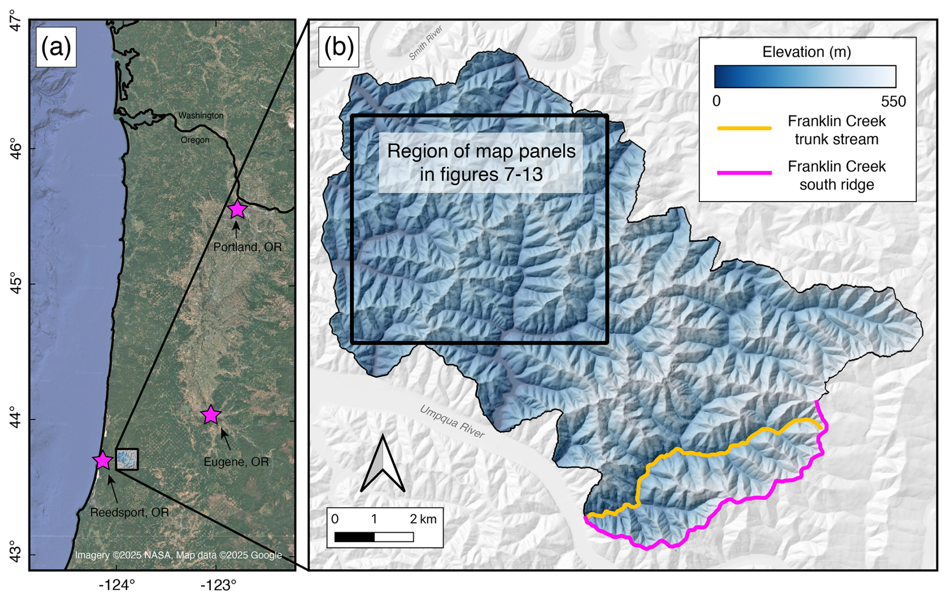
Figure 1 Map of study area. (a) Overview map of Cascadia coastal region showing the location of our study site. Satellite imagery is from Google Earth, accessed through QGIS XYZ tiles on 13 June 2025 (© 2025 Google. Map data licensed under the Google Maps/Google Earth Terms of Use; https://maps.google.com/help/terms_maps/, last access: 13 June 2025). (b) Elevation map of study area showing location of the Franklin Creek trunk stream and southern ridge of Franklin Creek basin analyzed in Sect. 5.3. Black outline shows region of focused maps in Figs. 8–14.

The Coast Range has long been studied as an archetypal steady-state landscape due to its uniform ridge-valley topography (Dietrich and Dunne, 1978; Montgomery, 2001) and correlations between drainage averaged erosion rates, uplift rates, and topographic proxies for erosion rate (Reneau and Dietrich, 1991; Heimsath et al., 2001; Struble et al., 2024). We focus on a small portion of the Coast Range with little variation in lithology (Baldwin, 1961; Beaulieu and Hughes, 1975) or climate (Daly et al., 2008). Owing to the relatively gentle dip of the bedrock, this area is not subject to deep-seated landslides that interrupt characteristic ridge-valley terrain in other portions of the Coast Range (LaHusen et al., 2020).

3 Definitions of curvature

3.1 Intrinsic versus extrinsic curvatures

Curvature formally refers to a class of mathematical operations that quantify deviations of a surface (or, more generally, a manifold) from flatness (Needham, 2021). Differential geometry and tensor calculus were in part developed to describe these operations (Pesic, 2007). Intrinsic curvatures are independent of coordinate system and can be calculated using only local surface information (Needham, 2021). Extrinsic curvatures are defined with respect to the ambient space in which the surface is embedded, and thus depend on the choice of external reference frame (Struik, 1950; O'Neill, 2006).

On DEMs, the accurate calculation of either intrinsic or extrinsic curvatures requires careful consideration of coordinates to avoid distortions that come from projection of topography onto a map grid. The effects of projection can be seen in Fig. 2, which compares the distances and angles of a map projection (Fig. 2a) to those of the same grid lines overlaying the 3-D surface (Fig. 2b). In the map-view representation, the E-W and N-S grid lines are perpendicular and evenly spaced. If one were to define displacement vectors dx and dy emanating from point p along these grid lines, their combination would create a resultant displacement ds^′ ending at point q^′. In Fig. 2b, however, displacement vectors du and dv, which connect p to the same points on the surface as dx and dy respectively, are not perpendicular and their combination results in a displacement (ds) that maps to a different point (q). Neighboring grid cells therefore have non-uniform dimensions and form non-orthogonal angles.

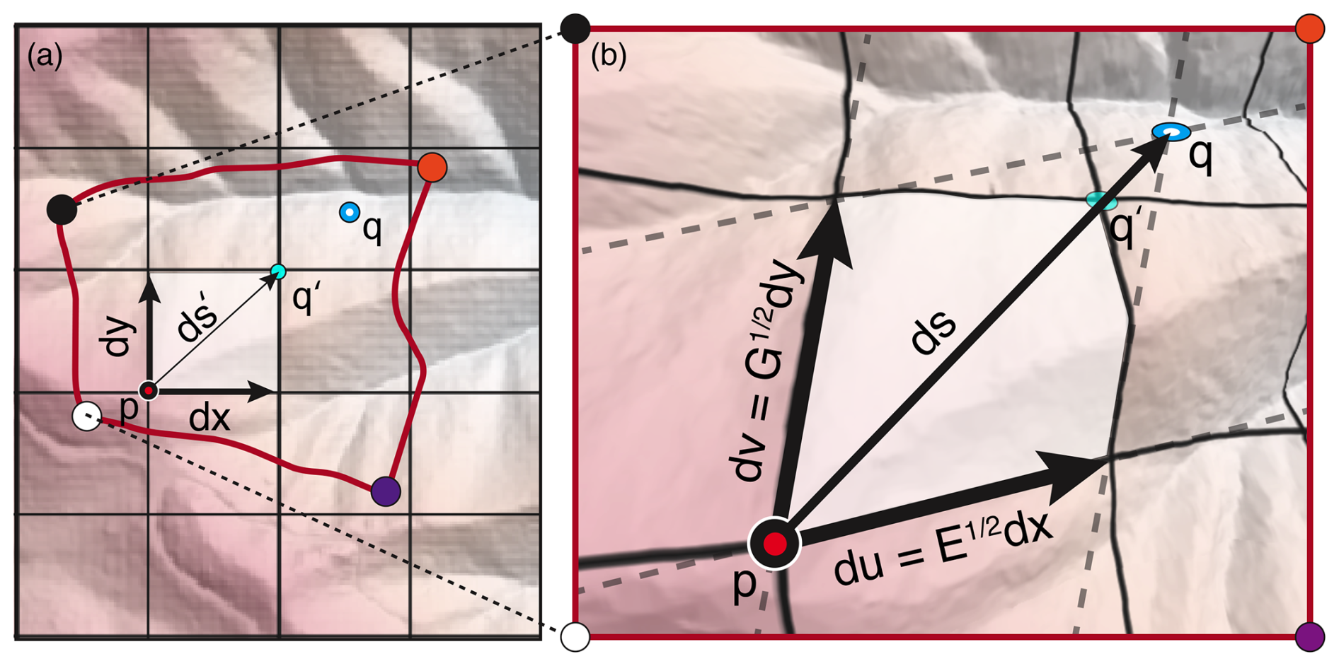
Figure 2 Difference between distances and angles measured on a map projection versus on the surface. (a) Map projection of DEM including map grid defined by E-W and N-S lines with grid spacing dx and dy. The red line corresponds to the rectangular outline in the adjacent panel. (b) DEM viewed as a 2-D manifold embedded in a 3-D space. Dashed lines show a locally defined uv coordinate system that follows x and y curves on the map projection, but which are not orthogonal or of equal length due to surface distortion. E and G are coefficients of the first fundamental form, and ds is the displacement vector that results from moving one grid space along each of these coordinate vectors.

Thus, accurate geometric calculations on topography require viewing a DEM not as a regular grid, but as a set of irregularly spaced data points sampling a surface, an approach that is similar in spirit to how elevation data are treated in landscape evolution models (Tucker et al., 2001). To accurately define a surface, distances and angles between grid cells are not treated as uniform quantities – they are computed locally within a reference frame defined at each point, reflecting the variation in surface geometry across the domain. This specific problem of topographic projection was recognized by Euler in 1775 and motivated the work of Gauss, who, roughly fifty years after Euler's observation, established the mathematical framework for accurate geometric classification of surfaces (Gauss, 1902; Needham, 2021). Using an approach similar to Gauss, we derive both intrinsic and extrinsic topographic curvature metrics built on invariant surface quantities.

3.2 Curvature invariants and related shape classes categories

At any point on a twice-differentiable surface, there exist two perpendicular directions along which the minimum and maximum normal curvatures occur (O'Neill, 2006). Between these directions, the curvature varies smoothly as

$$\begin{array}{}\text{(1)}& \mathit{\kappa }\left(\mathit{\theta }\right)=k_{\mathrm{1}}{\cos }^{\mathrm{2}}\mathit{\theta }+k_{\mathrm{2}}{\sin }^{\mathrm{2}}\mathit{\theta },\end{array}$$

where the extrema k₁ and k₂ are called the principal curvatures and θ is an angular direction measured within the surface tangent plane. Equation (1), known as Euler's Theorem, shows that the principal curvatures can be used to calculate normal curvature along any surface direction.

The principal curvatures can be used to calculate two other useful invariant quantities that will be more central to our analysis; the “mean” and “Gaussian” curvatures. The mean curvature, an extrinsic quantity, follows directly from Euler's Theorem and is the value about which the curvature oscillates as a function of angle on the surface (Eq. 1). While it can be calculated as the average curvature of any two perpendicular paths, we define it in terms of the principal curvatures as

$$\begin{array}{}\text{(2)}& K_{\mathrm{M}}={\displaystyle \frac{k_{\mathrm{1}}+k_{\mathrm{2}}}{\mathrm{2}}}.\end{array}$$

The Gaussian curvature (K_G) can be defined as the product of the principal curvatures

$$\begin{array}{}\text{(3)}& K_{\mathrm{G}}=k_{\mathrm{1}}{k}_{\mathrm{2}}.\end{array}$$

This value is intrinsic, meaning it is unchanged under isometric transformations and does not depend on the actual shape of the surface in space. Instead K_G captures a more subtle quality: the degree of stretching or bending required to deform a flat plane so that it conforms to the surface (O'Neill, 2006). Note that the units of K_G (m⁻²) are not the same as K_M (m⁻¹).

The mean and Gaussian curvatures together uniquely determine the local geometry as one of eight distinct shape classes (Bergbauer and Pollard, 2003; Fig. 3). Since the Gaussian curvature is the product of the two principal curvatures, it is positive only when k₁ and k₂ have the same sign. Positive K_G thus correlates to either domes or basins, though we cannot discern which from K_G alone. If K_G is negative, then k₁ and k₂ have opposing signs and the surface is locally a saddle. As with positive K_G, the orientation in space cannot be determined from this intrinsic quality. In cases where either k₁ or k₂ is equal to zero, K_G is also zero. Such shapes comprise a class of “developable surfaces”, which are intrinsically flat and can be formed from a plane without altering surface area. Curvature thresholding to extract developable forms (Mynatt et al., 2007) is a promising approach for classifying landforms. However, we do not explore this further here.

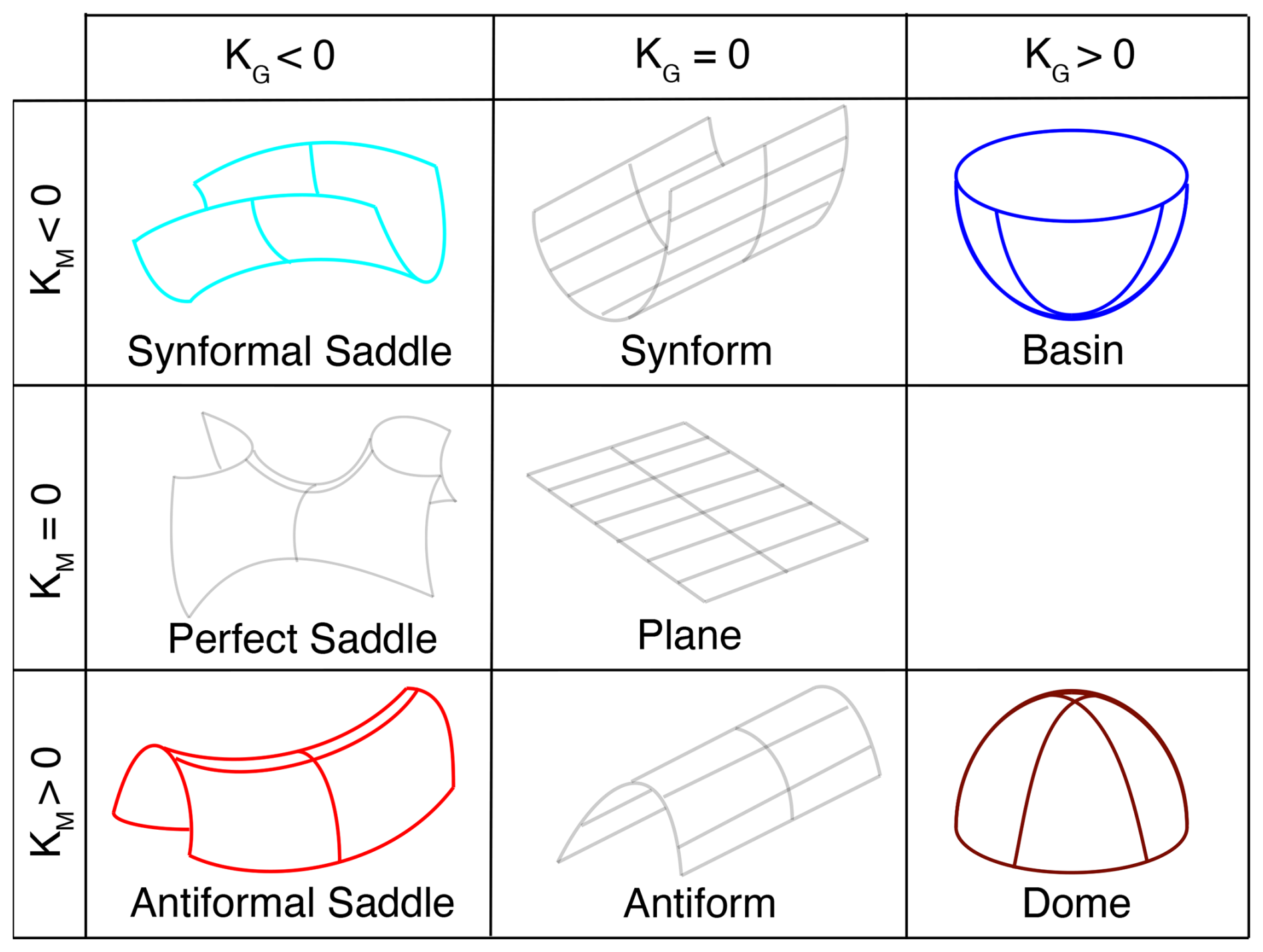
Figure 3 Shape classes into which points on the surface can be sorted based on the signs of the mean (K_M) and Gaussian (K_G) curvatures. In this analysis we focus on those classes that can be assigned based on raw curvature values, which are synformal saddles, antiformal saddles, basins, and domes, and do not include developable surfaces or perfect saddles. Modified from Mynatt et al. (2007).

The orientation of a shape is an extrinsic quantity that can be determined from the mean curvature, allowing us to put geometric classifications based on K_G into a landscape reference frame. This requires an arbitrary choice of positive curvature direction, which we choose to be positive for downward concavity consistent with differential geometry implementations in structural geology (Bergbauer and Pollard, 2003). K_M is positive in two cases: when both k₁ and k₂ are positive, or when the higher-magnitude curvature (k₁) is positive. This means that points in the landscape with K_M>0 are concave down and are locally either domes or antiformal saddles. Similarly, if K_M is negative, then the surface must be predominantly concave up and is either a basin or synformal saddle. More generally, the sign of the mean curvature allows us to differentiate between the divergence and convergence of surface gradient vectors.

3.3 Finding the principal curvatures

Defining curvature rigorously on discretely sampled topography requires accounting for changes in surface orientation between neighboring points, and how that change is scaled by non-uniform distances on a complicated surface. Our derivation of principal curvatures largely follows Struik (1950), though we point to complementary references throughout. A position on the surface is defined as the endpoint of a position vector parameterized by uv-coordinates such as those shown in Fig. 2b, but referenced to a Cartesian basis as

$$\begin{array}{}\text{(4)}& \mathit{r}(u,v)=r_{\mathrm{1}}{\widehat{\mathit{e}}}_{\mathrm{1}}+r_{\mathrm{2}}{\widehat{\mathit{e}}}_{\mathrm{2}}+r_{\mathrm{3}}{\widehat{\mathit{e}}}_{\mathrm{3}}\end{array}$$

where the ${\widehat{\mathit{e}}}_i$ are unit vectors corresponding to easting, northing, and elevation, and u and v are coordinates following any two intersecting curves on the surface. In this case the uv-coordinates follow the lines on the map-view grid, but we do not assume orthogonality on the surface. The square of the infinitesimal arc-length between points is given by

$$\begin{array}{}\text{(5)}& \mathbf{I}={\mathrm{ds}}^{\mathrm{2}}=\mathrm{d}\mathit{r}\cdot \mathrm{d}\mathit{r}=E\mathrm{d}{u}^{\mathrm{2}}+\mathrm{2}F\mathrm{d}u\mathrm{d}v+G\mathrm{d}{v}^{\mathrm{2}}\end{array}$$

where $E=\frac{\partial \mathit{r}}{\partial u}\cdot \frac{\partial \mathit{r}}{\partial u}$, $F=\frac{\partial \mathit{r}}{\partial u}\cdot \frac{\partial \mathit{r}}{\partial v}$, and $G=\frac{\partial \mathit{r}}{\partial v}\cdot \frac{\partial \mathit{r}}{\partial v}$ (the metric coefficients) quantify the proportionality of distances measured on the surface to distances in the Cartesian reference frame. They can also be used to calculate the ratio of area on the surface to pixel area as $\mathit{\alpha }=\sqrt{EG-F^{\mathrm{2}}}$, a quantity we will use to calculate intrinsic drainage areas in our analysis (Sect. 4).

Equation (5), known as the first fundamental form or surface metric formula, is used to calculate distances and areas on the surface. This in turn can be used to scale topographic curvatures. Curvatures are calculated as a change in surface orientation along a path, defined as

$$\begin{array}{}\text{(6)}& \mathbf{II}=\mathrm{d}\mathit{r}\cdot \mathit{N}=e\mathrm{d}{u}^{\mathrm{2}}+\mathrm{2}f\mathrm{d}u\mathrm{d}v+g\mathrm{d}{v}^{\mathrm{2}},\end{array}$$

where $e=\frac{{\partial }^{\mathrm{2}}\mathit{r}}{\partial u^{\mathrm{2}}}\cdot \mathit{N}$, $f=\frac{{\partial }^{\mathrm{2}}\mathit{r}}{\partial u\partial v}\cdot \mathit{N}$ and $g=\frac{{\partial }^{\mathrm{2}}\mathit{r}}{\partial v^{\mathrm{2}}}\cdot \mathit{N}$ (the curvature coefficients) are the projection of directional curvatures onto a unit normal vector

$$\begin{array}{}\text{(7)}& \mathit{N}={\displaystyle \frac{\frac{\partial \mathit{r}}{\partial u}\times \frac{\partial \mathit{r}}{\partial v}}{\left|\frac{\partial \mathit{r}}{\partial u}\times \frac{\partial \mathit{r}}{\partial v}\right|}}.\end{array}$$

Equation (6) is called the second fundamental form, and measures changes in the orientation of the tangent plane in the direction of ds. Combining the information in Eqs. (5) and (6) as

$$\begin{array}{}\text{(8)}& \mathit{\kappa }=-{\displaystyle \frac{\mathbf{II}}{\mathbf{I}}}=-{\displaystyle \frac{\mathrm{d}\mathit{r}}{\mathrm{ds}}}\cdot {\displaystyle \frac{\mathrm{d}\mathit{N}}{\mathrm{ds}}}=-{\displaystyle \frac{e\mathrm{d}{u}^{\mathrm{2}}+\mathrm{2}f\mathrm{d}u\mathrm{d}v+g\mathrm{d}{v}^{\mathrm{2}}}{E\mathrm{d}{u}^{\mathrm{2}}+\mathrm{2}F\mathrm{d}u\mathrm{d}v+G\mathrm{d}{v}^{\mathrm{2}}}}\end{array}$$

allows us to fully characterize the local shape of a surface in 3-D space. The coefficients of the second fundamental form (e, f and g; Eq. 6) are the directional curvatures where e and g correspond to curvature along the E-W and N-S grid lines respectively, and f is a cross term that accounts for directional covariance. These values are scaled by the coefficients of the first fundamental form (E, F, and G; Eq. 5), which maps lengths on the coordinate grid to lengths on the surface.

The directions of the principal curvatures can be found algebraically by defining a parameter $\mathit{\lambda }=\mathrm{d}v/\mathrm{d}u$ and rewriting Eq. (8) as

$$\begin{array}{}\text{(9)}& \begin{array}{rl}\mathit{\kappa }\left(\mathit{\lambda }\right)& ={\displaystyle \frac{e\mathrm{d}{u}^{\mathrm{2}}+\mathrm{2}f\mathit{\lambda }\mathrm{d}{u}^{\mathrm{2}}+g{\mathit{\lambda }}^{\mathrm{2}}\mathrm{d}{u}^{\mathrm{2}}}{E\mathrm{d}{u}^{\mathrm{2}}+\mathrm{2}F\mathit{\lambda }\mathrm{d}{u}^{\mathrm{2}}+G{\mathit{\lambda }}^{\mathrm{2}}\mathrm{d}{u}^{\mathrm{2}}}}\\ & ={\displaystyle \frac{e+\mathrm{2}f\mathit{\lambda }+g{\mathit{\lambda }}^{\mathrm{2}}}{E+\mathrm{2}F\mathit{\lambda }+G{\mathit{\lambda }}^{\mathrm{2}}}}.\end{array}\end{array}$$

Since the principal curvatures correspond to extrema where $\mathrm{d}\mathit{\kappa }/\mathrm{d}\mathit{\lambda }=\mathrm{0}$ we differentiate Eq. (9) with respect to λ and set the result equal to zero giving

$$\begin{array}{}\text{(10)}& \begin{array}{rl}{\displaystyle \frac{\mathrm{d}\mathit{\kappa }}{\mathrm{d}\mathit{\lambda }}}=& \left(E+\mathrm{2}F\mathit{\lambda }+G{\mathit{\lambda }}^{\mathrm{2}}\right)(f+g\mathit{\lambda })\\ & -\left(e+\mathrm{2}f\mathit{\lambda }+g{\mathit{\lambda }}^{\mathrm{2}}\right)(F+G\mathit{\lambda })=\mathrm{0},\end{array}\end{array}$$

a quadratic equation in λ whose roots correspond to the principal curvature directions. Recalling that $\mathit{\lambda }=\mathrm{d}v/\mathrm{d}u$ these values can be equated to angles in our local uv-coordinate system and can thus reference principal curvature orientations within the map-view grid.

Magnitudes of the principal curvatures are found through a similar approach. Since $\mathrm{d}\mathit{\kappa }/\mathrm{d}\mathit{\lambda }=\mathrm{0}$ along the principal directions, Eqs. (9) and (10) are combined to give a simpler expression for the curvature

$$\begin{array}{}\text{(11)}& \mathit{\kappa }={\displaystyle \frac{f+g\mathit{\lambda }}{F+G\mathit{\lambda }}}.\end{array}$$

Recognizing that

$$\begin{array}{}\text{(12)}& E+\mathrm{2}F\mathit{\lambda }+G{\mathit{\lambda }}^{\mathrm{2}}=(E+F\mathit{\lambda })+\mathit{\lambda }(F+G\mathit{\lambda })\end{array}$$

and

$$\begin{array}{}\text{(13)}& e+\mathrm{2}f\mathit{\lambda }+g{\mathit{\lambda }}^{\mathrm{2}}=(e+f\mathit{\lambda })+\mathit{\lambda }(f+g\mathit{\lambda }),\end{array}$$

Eq. (10) can be rearranged to show

$$\begin{array}{}\text{(14)}& \mathit{\kappa }={\displaystyle \frac{f+g\mathit{\lambda }}{F+G\mathit{\lambda }}}={\displaystyle \frac{e+f\mathit{\lambda }}{E+F\mathit{\lambda }}}.\end{array}$$

The two expression for curvature given by Eq. (14) are rearranged as

$$\begin{array}{}\text{(15)}& f-\mathit{\kappa }F+\mathit{\lambda }(g-\mathit{\kappa }G)=\mathrm{0}\end{array}$$

and

$$\begin{array}{}\text{(16)}& e-\mathit{\kappa }E+f-\mathit{\kappa }F=\mathrm{0},\end{array}$$

respectively. Multiplying Eqs. (15) and (16) by du (with $\mathit{\lambda }=\mathrm{d}v/\mathrm{d}u$) we arrive at a system of linear equations in our original uv-coordinate system

$$\begin{array}{}\text{(17)}& \left[\begin{array}{cc}e-\mathit{\kappa }E& f-\mathit{\kappa }F\\ f-\mathit{\kappa }F& g-\mathit{\kappa }G\end{array}\right]\left[\begin{array}{c}\mathrm{d}u\\ \mathrm{d}v\end{array}\right]=\left[\begin{array}{c}\mathrm{0}\\ \mathrm{0}\end{array}\right].\end{array}$$

This has a non-trivial solution only if the determinant of the coefficient matrix is zero. The corresponding quadratic equation in κ

$$\begin{array}{}\text{(18)}& (EG-F^{\mathrm{2}}){\mathit{\kappa }}^{\mathrm{2}}-(gE-\mathrm{2}fF+eG)\mathit{\kappa }+(eg-f^{\mathrm{2}})=\mathrm{0}\end{array}$$

has roots that are the principal curvatures. By convention, we take the more positive of these roots to be k₁, while the less positive curvature is k₂.

4 Computing curvatures on gridded DEMs

4.1 Spectral filtering of gridded datasets

To calculate DEM curvatures, it is necessary to do some degree of smoothing to remove artifacts of the gridding process (Reuter et al., 2009; Bui and Glennie, 2023; Bater and Coops, 2009). We use 8.1 m resolution DEM data freely available through the National Map (https://apps.nationalmap.gov/downloader/, last access: 16 November 2024). While higher resolution LiDAR (Light Detection and Ranging) data are available in the study area, the coarser dataset is sufficient for resolving geometric trends and ridge-valley landforms at the scale of fluvial basins.

There are many established approaches to DEM smoothing, including b-spline fitting (Brigham and Crider, 2022), wavelets (Struble et al., 2024), selective denoising (Gallant, 2011), and TIN interpolation (Jordan, 2007). We choose to filter the data using a Discrete Fourier Transform (DFT; also a contribution of Gauss; Heideman et al., 1985), which decomposes discretely sampled signals into sums of harmonic functions. Smoothing is accomplished via low-pass filtering, where information at wavelengths smaller than a defined cutoff is removed. Fourier methods have been extensively applied in geomorphology toward the identification of characteristic process scales (Perron et al., 2008), landform classification (Booth et al., 2009), and the assessment of topographic controls on mass transport mechanics (Richardson and Karlstrom, 2019; Black et al., 2017; Crozier et al., 2018).

One challenge of Fourier methods is that harmonic functions do not naturally respect the finite nature of a DEM. Tapering of the data is thus required to obtain zero elevation at the boundaries prior to applying a DFT. It is common to accomplish this by convolving the DEM grid with a 2-D raised cosine (aka Hanning window), such that the resulting topography is equal to its actual value only at center of the grid, and approaches zero at the margins (Perron et al., 2008).

A downside of this approach is that it does not preserve the spectral power of landscape features. Fortunately, this effect can be minimized by first reflecting the topographic grid along each coordinate axis, then tapering the data only in reflected portions that fall outside the limits of the original DEM (Mcnutt, 1983; Harris, 1978). While spurious signals at wavelengths greater than the DEM are not eliminated, this windowing approach minimizes smaller scale distortion within the study area. We use a Tukey window (implemented as window2 in Matlab), which consists of a boxcar function convolved with a cosine taper along the margins (Harris, 1978).

The Discrete Fourier Transform (DFT) is calculated as

$$\begin{array}{}\text{(19)}& Z(k_x,k_y)=\sum _{p=\mathrm{0}}^{N_x-\mathrm{1}}\sum _{q=\mathrm{0}}^{N_y-\mathrm{1}}z\left(p\mathrm{\Delta }x,q\mathrm{\Delta }y\right)e^{-\mathrm{2}\mathit{\pi }i\left(\frac{k_{x}p}{N_x}+\frac{k_{y}q}{Ny}\right)},\end{array}$$

where N_x and N_y are the number of grid cells in each direction, p and q are array indices, Δx and Δy are the grid spacings in each direction, and k_x and k_y are the wavenumbers in the respective x and y directions (Perron et al., 2008). Each value in the output array given by the above equation is associated with a frequency in x and y directions with magnitudes

$$\begin{array}{}\text{(20)}& f_x={\displaystyle \frac{k_x}{N_x\mathrm{\Delta }x}},f_y={\displaystyle \frac{k_y}{N_y\mathrm{\Delta }y}}.\end{array}$$

These frequencies can then be used to define a radial frequency as

$$\begin{array}{}\text{(21)}& f_{\mathrm{r}}=\sqrt{f_x^{\mathrm{2}}+f_y^{\mathrm{2}}}.\end{array}$$

The DFT periodogram is then given by

$$\begin{array}{}\text{(22)}& P_f(k_x,k_y)={\displaystyle \frac{\mathrm{1}}{N_x^{\mathrm{2}}{N}_y^{\mathrm{2}}}}\left|Z\right(k_x,k_y){|}^{\mathrm{2}}\end{array}$$

Following Perron et al. (2008) we apply a half-Gaussian filter based on radial frequencies

$$\begin{array}{}\text{(23)}& F_{\mathrm{low}}=\left\{\begin{array}{ll}\mathrm{1},& f<f_{\mathrm{1}},\\ \exp \left(\frac{-(f-f_{\mathrm{1}}{)}^{\mathrm{2}}}{\mathrm{2}{\mathit{\sigma }}^{\mathrm{2}}}\right),& f\ge f_{\mathrm{1}},\end{array}\right.\end{array}$$

where $\mathit{\sigma }=\frac{\mathrm{1}}{\mathrm{3}}|f_{\mathrm{2}}-f_{\mathrm{1}}|$ is the standard deviation. The filter is convolved with the radial frequency spectrum before the filtered spectrum is reverse transformed and the original domain of the DEM is extracted from the windowed representation to yield a low-pass filtered raster of topography.

4.2 Selection of filtering scale

Once the landscape has been filtered, the invariant curvature metrics outlined in Sect. 3.2 and 3.3 are calculated on each DEM pixel. Curvature values are binned by drainage surface-area, calculated using the D-infinity algorithm (Tarboton, 1997) implemented in the TopoToolbox MATLAB function library (Schwanghart and Scherler, 2014), with pixel values weighted by the surface area ratio (α) defined in Sect. 3.3.

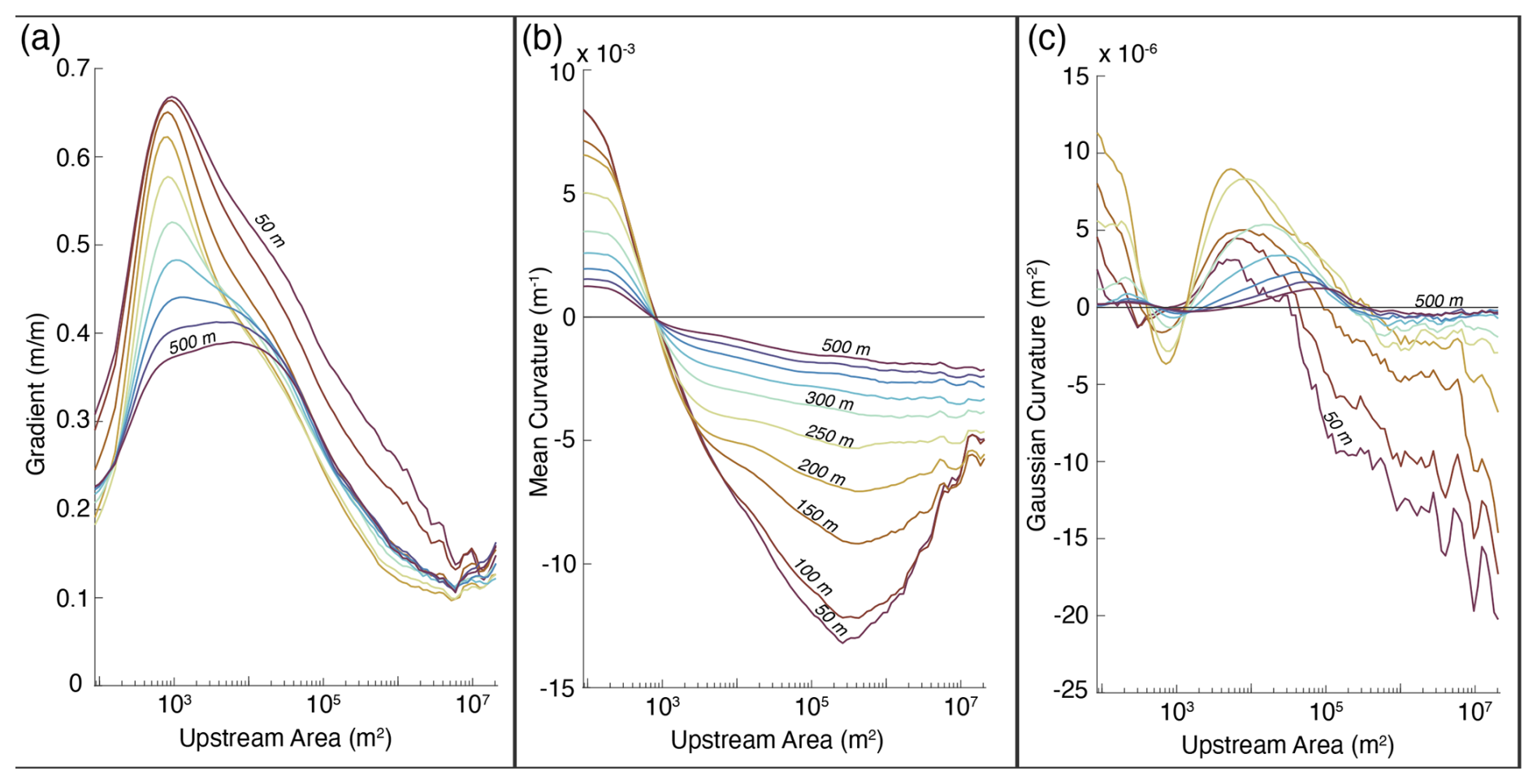
Figure 4 Surface geometry metrics binned by upstream drainage area for a range of low-pass filter cut-offs between 50 and 500 m calculated on 50 m intervals. (a) Gradient of tangent plane. (b) Mean curvature (K_M). (c) Gaussian curvature (K_G).

To explore the impact of low pass filter scale, we first smooth the landscape to 50 m, then increase the low-pass filter cutoff by increments of 50 up to 500 m and look for shifting patterns in the area-space evolution of topographic geometry (Fig. 4). While the magnitudes of curvature and slope vary with increased filtering, general trends in these metrics are similar across this range of filter cutoffs. This suggests that the filter cutoff parameter does not strongly alter landscape geometric structure. However, while the magnitudes of mean curvature decrease systematically with increasing filter cutoff, the main extrema in Gaussian curvature have the greatest magnitudes at a cutoff of 200 m, perhaps indicating a characteristic curvature scale in the landscape.

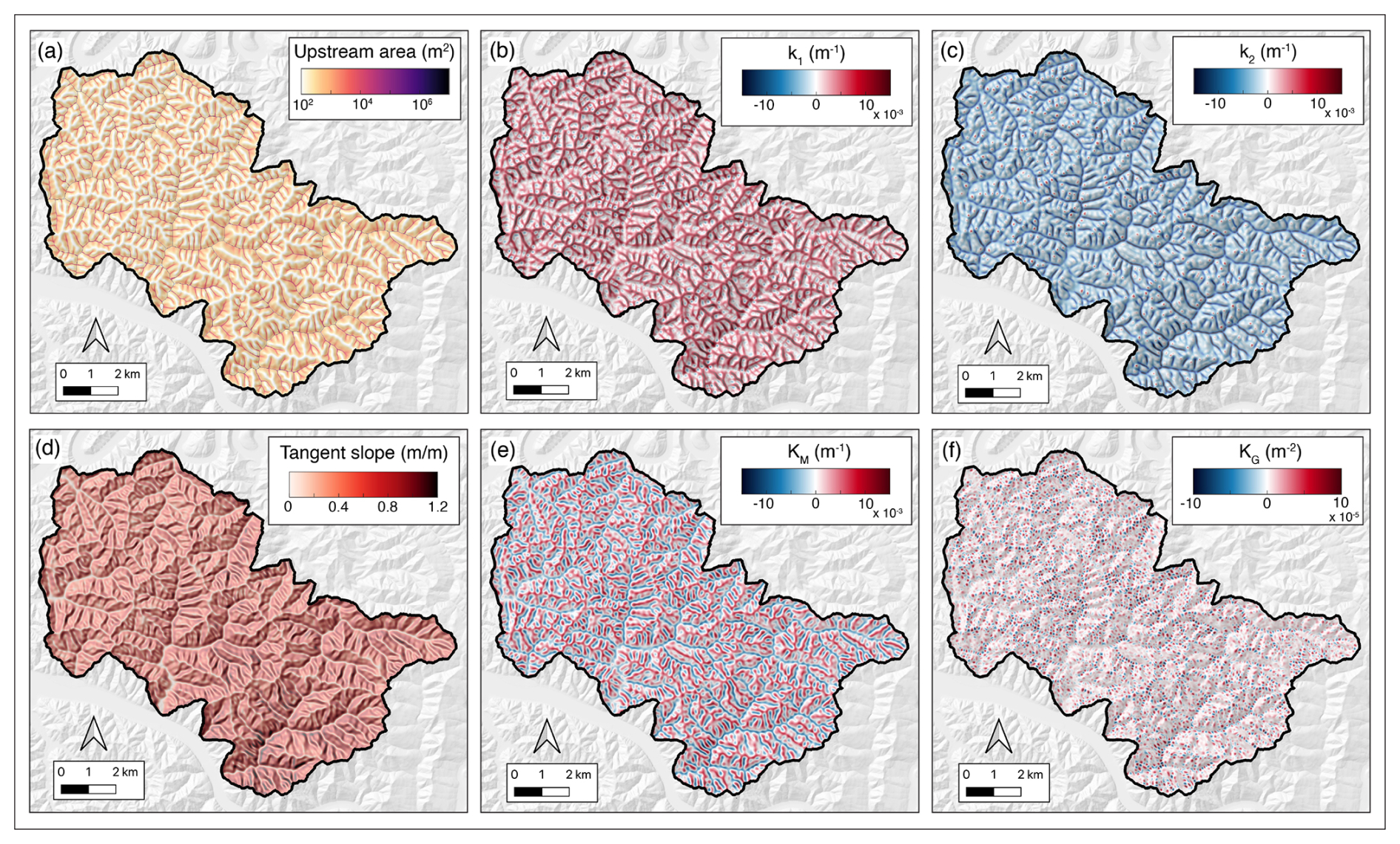
Figure 5 Map-view distributions of surface geometry metrics. (a) drainage area of grid points calculated with D-infinity algorithm. Pixels are weighted with area-ratio α to reflect drainage area on the topographic surface rather than the map-view projection. (b) First principal curvature (k₁). (c) Second principal curvature (k₂). (d) Slope of tangent plane (S_T). (e) Mean curvature (K_M). (f) Gaussian curvature (K_G).

Based on these observations, we perform all further analysis on topography low-pass filtered to 200 m. This filter scale allows us to identify landscape features that span hillslope and fluvial process regimes, but inhibits our ability to analyze topography at finer scales. Map-view distributions of mean and Gaussian curvatures, principal curvatures, tangent plane slope, and upstream drainage area for a DEM filtered to 200 m are shown in Fig. 5. The MATLAB code used to filter and compute curvatures on the landscape is publicly available (Klema and Karlstrom, 2026), in addition to a Python implementation (Schermer et al., 2026).

4.3 Comparison to common topographic metrics

In this work, we have proposed a geometrically self-consistent framework for defining topography through connection to formal surface theory. A benefit of intrinsic geometric methods is that they eliminate the projection distortion of surface properties computed in map-view, which is the most common way to calculate topographic slope and curvature. The severity of such projection distortion depends on the geometry of the surface itself, as map-view approximations are quite valid in low-slope regions but are less so in steep topography. Below, we compare our method to these common approaches and quantify where on landscapes the intrinsic geometric perspective is likely informative.

4.3.1 Comparison of mean and projected Laplacian curvatures

Formally, the Laplacian of a single-valued curved surface z(x,y) is given by the Laplace-Beltrami operator, which yields

$$\begin{array}{}\text{(24)}& \mathrm{2}{K}_{\mathrm{M}}=\mathrm{\nabla }\cdot \left({\displaystyle \frac{\mathrm{\nabla }z}{\sqrt{\mathrm{1}+|\mathrm{\nabla }z{|}^{\mathrm{2}}}}}\right)\end{array}$$

regardless of slope (O'Neill, 2006). Expanding Eq. (24) in a Taylor series about the point $|\mathrm{\nabla }z{|}^{\mathrm{2}}=\mathrm{0}$ gives

$$\begin{array}{}\text{(25)}& \mathrm{2}{K}_{\mathrm{M}}={\mathrm{\nabla }}^{\mathrm{2}}z-{\displaystyle \frac{\mathrm{1}}{\mathrm{2}}}\mathrm{\nabla }\cdot \left(|\mathrm{\nabla }z{|}^{\mathrm{2}}\mathrm{\nabla }z\right)+{\displaystyle \frac{\mathrm{3}}{\mathrm{8}}}\mathrm{\nabla }\cdot \left(|\mathrm{\nabla }z{|}^{\mathrm{4}}\mathrm{\nabla }z\right)-\mathrm{\cdots },\end{array}$$

which reduces to the Laplacian for a Euclidean metric (∇²z), as $\left|\mathrm{\nabla }z\right|\to \mathrm{0}$. Equation (25) is the basis for the small-slope approximation in geomorphology, wherein soil diffusion is taken as proportional to ∇²z on hilltops, and higher-order terms are associated with non-linear behavior on steep hillslopes (Andrews and Bucknam, 1987). The mean curvature, however, is valid regardless of slope and thus captures the geometry of both linear and non-linear hillslope regions. Figure 6 compares $\frac{\mathrm{1}}{\mathrm{2}}{\mathrm{\nabla }}^{\mathrm{2}}z$ calculated on a coordinate grid to the invariant mean curvature K_M. We first compare on a unit hemisphere (Fig. 6a–b) and then on binned topographic data in the Oregon Coast Range study site (Fig. 6c).

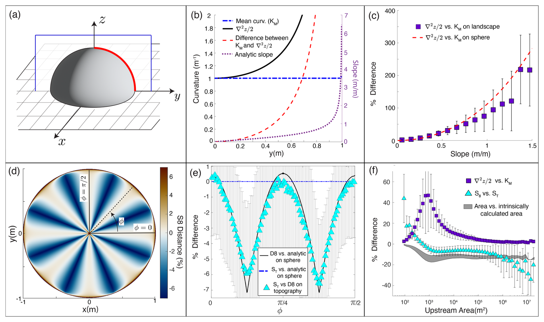
Figure 6 Comparison of intrinsic surface metrics use in this study with other methods common in the literature. (a) The unit hemisphere used for comparison with topographic data. Red line shows curve along which error is evaluated in panel (b). (b) Comparison of mean curvature (K_M) and ${\mathrm{\nabla }}^{\mathrm{2}}z/\mathrm{2}$ (half the projeted Laplacian curvature) as a function of distance from the origin for plane curve defined by the intersection of the unit hemisphere with the y−z plane. Black line is ${\mathrm{\nabla }}^{\mathrm{2}}z/\mathrm{2}$, blue dashed line is mean curvature calculated using intrinsic method, red dashed line is difference between ${\mathrm{\nabla }}^{\mathrm{2}}z/\mathrm{2}$ and the curvature of the sphere (1 m⁻¹). The purple dashed line is surface slope. (c) Percent error of ${\mathrm{\nabla }}^{\mathrm{2}}z/\mathrm{2}$ on the unit hemisphere and % difference between ${\mathrm{\nabla }}^{\mathrm{2}}z/\mathrm{2}$ and mean curvature on topography binned as a function of slope. Red dashed line is % error on sphere and purple boxes are median values computed on topography. (d) Percent error of the 8-point connected gradient computed on the unit hemisphere. (e) % error of the 8 point connected gradient computed on the unit hemisphere and median % difference between S₈ and S_T as a function of azimuth. (f) Intrinsically calculated curvature (Sect. 4.3.1), slope (Sect. 4.3.2), and upstream area (Sect. 4.3.3) versus common DEM-derived metrics, as a function of drainage area.

Deviation of $\frac{\mathrm{1}}{\mathrm{2}}{\mathrm{\nabla }}^{\mathrm{2}}$ from the mean curvature is dramatic in end-member cases, but is negligible in many applications. It can be strategically avoided by focusing on low-slope regions (Hurst et al., 2012), or evaluating curvature along 1-D hillslope profiles in which it is easier to account for slope effects (Roering et al., 2007). A formal approach, however, has potential to strengthen such studies. In reality, there are few points in the landscape with zero slope. For example, the hilltop region identified in this study makes up 18 % of the landscape (Sect. 5.1.1; Fig. 9). Roughly half of this subset is along steep ridge lines with slopes above 0.4, where slope distortion in the Laplacian is around 20 % (Fig. 6b–c). Selecting lower slope thresholds increases accuracy, but at the cost of data volume, a tradeoff that does not need to be considered with intrinsic approaches. Quantifying the difference in these values also measures the degree to which non-linear processes increase with slope, as ∇²z represents the linear term (Roering et al., 2001a).

4.3.2 Comparison of tangent slope to 8-connected neighborhood gradient

Our approach to computing curvatures requires definition of a unit normal vector at every DEM grid cell, which also defines the slope of the local tangent plane (S_T). We compare this method, which is mathematically equivalent to finding a slope magnitude using the Pythagorean sum of directional derivatives, to the commonly used 8-connected neighborhood gradient (D8) that is the default in some landscape analysis toolboxes (Schwanghart and Scherler, 2014; Mudd et al., 2019). The D8 method assigns a given pixel the slope between it and its lowest neighbor, providing an efficient flow routing algorithm (O'Callaghan and Mark, 1984). Figure 6d shows the percent difference between the D8 algorithm and tangent slope on a projection of the unit sphere. In Fig. 6e we this deviation by azimuth (black line) and presents a comparison with both S_T on the sphere (blue dashed line), and the difference between S_T and D8 on topography (cyan triangles).

Differences between D8-values and the analytic slope vary systematically with orientation of the surface up to magnitudes of ∼ 7 %. The percent error in S_T on the sphere is near zero, while the differences between the various slope metrics on topography track the same azimuthal trend. This arises because the D8-algorithm tends to underestimate slope if pixels are misaligned with the direction of steepest descent. We bin the percent difference between S_T and D8 by drainage area to track differences in the two metrics through the fluvial network (Fig. 6f). The highest magnitude errors (∼ 35 %) occur on ridges (Sect. 5.1.1), while the largest negative errors (exceeding 20 %) occur within the fluvial network (Sect. 5.1.4). Correlation with K_M (Fig. 8) suggests sensitivity of the D8-algorithm to surface curvature as well as orientation. This has implications for tectonic geomorphology studies that make inference from slope values between landscape regions.

4.3.3 Drainage surface area versus map-view area

As outlined in Sect. 3, this work is partially motivated by the fact that distances and areas on a sloped surface are greater than on their map-view representations. Specifically, the ratio of surface to pixel area can be calculated using the metric coefficients as $\mathit{\alpha }=\sqrt{EG-F^{\mathrm{2}}}$. To evaluate the effect of projection on drainage area values, we compute two separate area grids using the D-infinity flow routing algorithm in TopoToolbox (Schwanghart and Scherler, 2014), one with uniform pixel dimensions and another where pixels are weighted by α. We bin the percent difference between these values by drainage area, with results shown in Fig. 6f. Through most of the landscape, extrinsic drainage area calculations underestimate drainage surface area by 10 %–15 %.

There is an extensive literature on drainage area calculation, and drainage values are known to be sensitive to grid resolution (Bernard et al., 2022), filtering scale (Erdbrügger et al., 2021), and the choice of flow routing algorithm (Tarboton, 1997). It is beyond the scope of this study to systematically integrate our intrinsic approach with other sensitivities. We note that true land surface area is derivable from DEMs, and could be beneficial in some applications. For example, efforts to define drainage-scale hydrologic responses to snow melt in mountain basins depend on estimated snow water equivalent values interpolated over topography (Chen et al., 2022; Acharki et al., 2025); models that consider groundwater infiltration and soil carbon sequestration in addition to overland flow contain parameters that depend on land surface area (Taherian and Ameli, 2026; Hunter et al., 2024); and certain definitions of characteristic topographic length scales depend on measures of area accumulation defined on the surface (Gallant and Hutchinson, 2011; Grieve et al., 2016). In each of these cases, the ability to accurately define surface area from map-view DEMs could be beneficial, though efforts to implement true surface area into process models are sometimes inappropriate (e.g. Iverson and George, 2024).

5 A geometric view of Coast Range topography

As outlined in Sect. 3.2, mean and Gaussian curvature values can be used to classify each DEM pixel uniquely into four distinct shape classes: dome, basin, synformal saddle, and antiformal saddle (Fig. 3). Upstream drainage area provides a natural way to study the resulting shape class distributions across the landscape, represented in Fig. 7a by its probability density function (PDF). Figure 7b shows PDFs of each shape class, which represents the probability of a shape class and given drainage area value occurring simultaneously (P(C∩A)). As the distribution of shapes is clearly weighted by the area distribution, we find it more informative to calculate the conditional probabilities of shapes classes (Fig. 7c) by invoking the probability axiom

$$\begin{array}{}\text{(26)}& P(C\cap A)=P\left(C\right|A\left)P\right(A)\to P(C\left|A\right)={\displaystyle \frac{P(C\cap A)}{P\left(A\right)}},\end{array}$$

where P(C|A) is the conditional probability of shape class occurring given a value of A, and P(A) is the probability of pixel having a drainage area A.

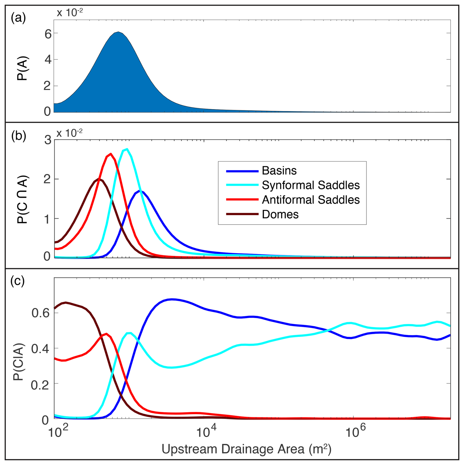
Figure 7 Shape class distributions as a function of drainage area. (a) Probability density function of drainage areas within the region of interest. (b) Probability density functions of shape classes as a function of drainage area. (c) Conditional PDFs of shape classes at a given drainage area.

Figure 8 shows a compilation of basic geometric data extracted through our approach, represented in both area-space and map-view perspectives. While other potentially useful information can be extracted using this approach (such as the orientations and magnitudes of k₁ and k₂), we focus largely on curvature invariants to demonstrate the utility of curvature for identifying distinctive geometric properties of fluvial topography.

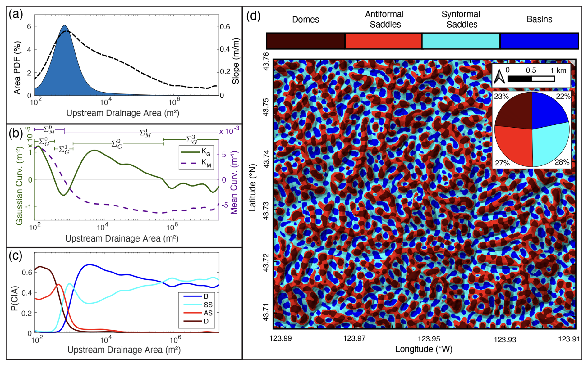
Figure 8 Distribution of derived surface geometry metrics computed on the full region of interest. (a) PDF of upstream drainage areas. Black dashed curve is slope binned by drainage area. (b) Gaussian and mean curvatures binned by drainage area. Horizontal lines at top of panel show Σ regions outlined in Sect. 5.1 and 5.2. (c) Conditional PDFs of shape classes as a function of drainage area. (d) Map of shape classes projected on a focused subregion of the study area. Pie-chart inset shows shape-class composition of the surface.

5.1 Landscape partitioning from Gaussian curvature

Noting significant and systematic variation in shape class distributions and curvature metrics with upstream drainage area (Fig. 8a–c), we now explore landscape segmentation using inflection points in the mean and Gaussian curvatures. This is motivated by the physical assumption that signs of both K_M and K_G have implications for mass transport phenomena. The sign of K_M records the divergence versus convergence of local gradients, while the sign of K_G differentiates between stable and unstable “critical points” that influence how the surface responds to disturbances (Calkin, 1996; Matsumoto, 2001; Bonetti et al., 2018). As our partitioning approach is rooted in geometry, we choose a labeling scheme ${\mathrm{\Sigma }}_i^j$ based solely on curvature invariants. Subscripts indicate the curvature used (i=G for K_G and i=M for K_M), while superscripts (j) correspond to the number of previous zero crossings in area space (j=0 corresponds to zero drainage area).

5.1.1 ${\mathrm{\Sigma }}_{\mathrm{G}}^{\mathrm{0}}$: drainage areas less than 3.75×10² m²

In fluvial landscapes, the smallest drainage areas are associated with the ridge-peak networks separating neighboring watersheds (Scherler and Schwanghart, 2020). We define a landscape region (${\mathrm{\Sigma }}_{\mathrm{G}}^{\mathrm{0}}$) containing pixels with drainage areas less than 3.75×10² m², the first area-space inflection in Gaussian curvature (Fig. 9b). In this region, both curvature invariants are dominantly positive, reflecting downward concavity of topography and the divergence of surface gradient vectors (Dietrich et al., 1993; O'Neill, 2006). This is consistent with a region lacking convergent overland flow (Fenneman, 1908), where mass transport is accomplished through diffusive hillslope-transport processes. Large positive mean curvature here suggests high rates of diffusion required for erosion along ridge lines to keep pace with mass transport in channel networks below (Roering et al., 1999). This is supported by correlations between Laplacian curvature of hilltop regions and drainage-scale erosion rates elsewhere in the Oregon Coast Range (Struble et al., 2024).

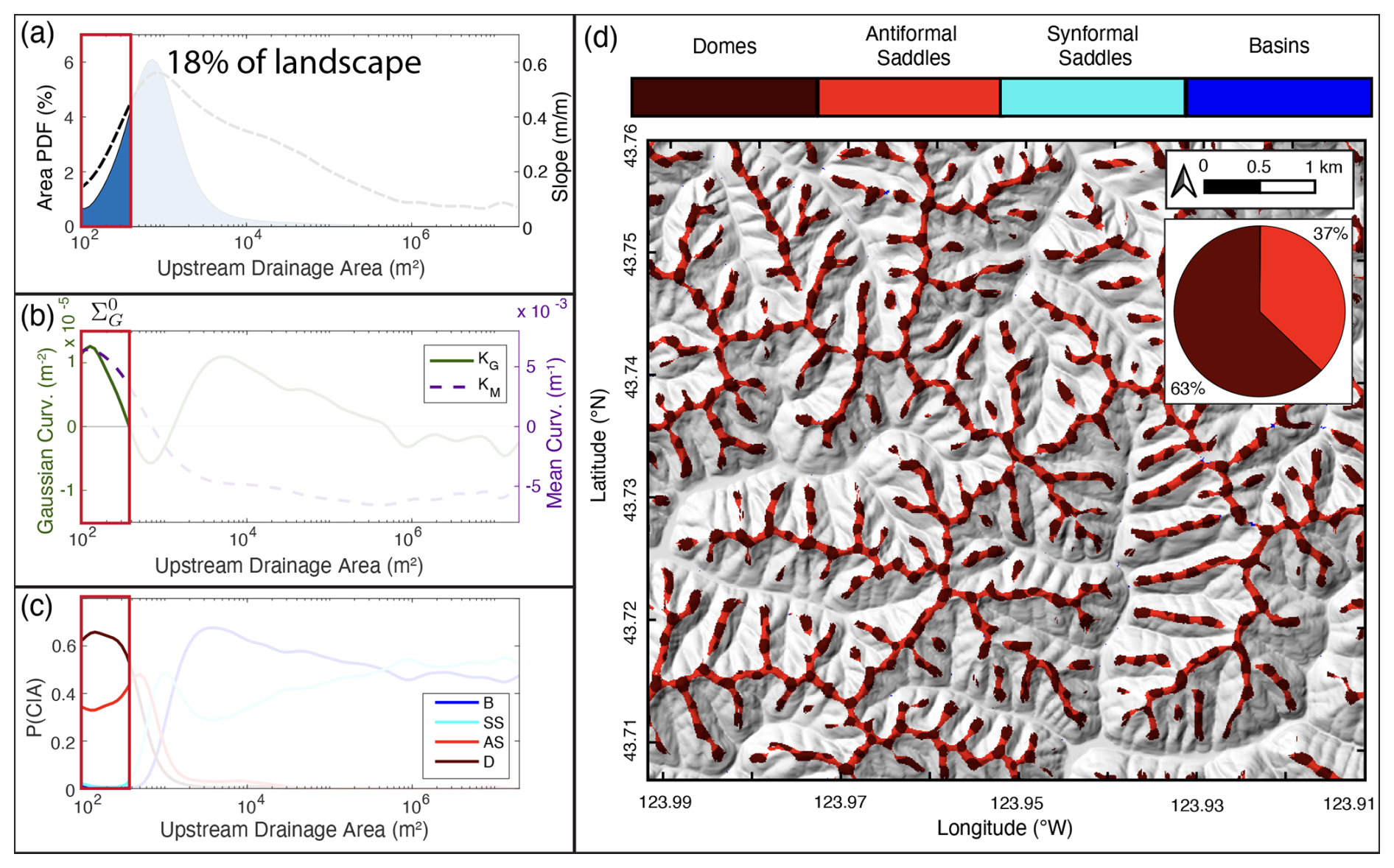
Figure 9 Surface geometry data for region ${\mathrm{\Sigma }}_{\mathrm{G}}^{\mathrm{0}}$: points in the landscape with upstream drainage areas less than 3.75×10² m². The red box in each of the area-binned plots (a–c) highlights the range of included drainage areas. (a) PDF of drainage areas. (b) Gaussian and mean curvatures binned by area. (c) Conditional PDFs of shape classes. (d) Map of shape classes projected on a focused subregion of the study area. Pie-chart inset shows shape-class composition of the surface.

Defined this way, the ridge-peak network makes up 18 % of the land-surface (to 2 significant figures). Within this subregion, 63 % of points are domal (peaks), with antiformal saddles (ridges) comprising the remaining 37 % (Fig. 9a, d). Along ridge lines this is expressed in oscillations between positive and negative Gaussian curvatures, analogous to the alternating “summits” and “knots” of Cayley (1859), and the “hills” and “passes” of Maxwell (1870). We will elaborate on this connection to early landscape organization theories in Sect. 5.3.

5.1.2 ${\mathrm{\Sigma }}_{\mathrm{G}}^{\mathrm{1}}$: Drainage areas between 3.75×10² and 1.29×10³ m²

As drainage area increases above 3.75×10² m², the binned Gaussian curvature changes sign and is negative up to areas of 1.29×10³ m² (Fig. 10b). 57 % of the land surface falls within this relatively narrow range of drainage areas, making it the largest of the ${\mathrm{\Sigma }}_{\mathrm{G}}^j$. This region is defined by high topographic gradients (Fig. 10a), coinciding with hillslopes where loose material moves downhill through a combination of gradient-driven landsliding, granular creep, and stochastic raveling (Roering et al., 2001b; Jaeger and Nagel, 1992; Furbish et al., 2009; Deshpande et al., 2021; Gabet, 2003). Within this region, the point of minimum K_G coincides with the highest slopes in the landscape. It is associated with the only inflection point in mean curvature, marking the dominant concavity transition in the landscape. Such a concavity transition is required to connect almost uniformly divergent topography on hilltops (${\mathrm{\Sigma }}_{\mathrm{G}}^{\mathrm{0}}$; Sect. 5.1.1) to convergent basins at the head of the drainage network (${\mathrm{\Sigma }}_{\mathrm{G}}^{\mathrm{2}}$; Sect. 5.1.3). Geometrically, this manifests as rapid shape-class changes over a small range of drainage area (Fig. 10c) and a more even split between the four shape classes overall (each shape class occupies ∼ 10 %–30 % of the region), which suggests a high level of surface complexity across this concavity transition.

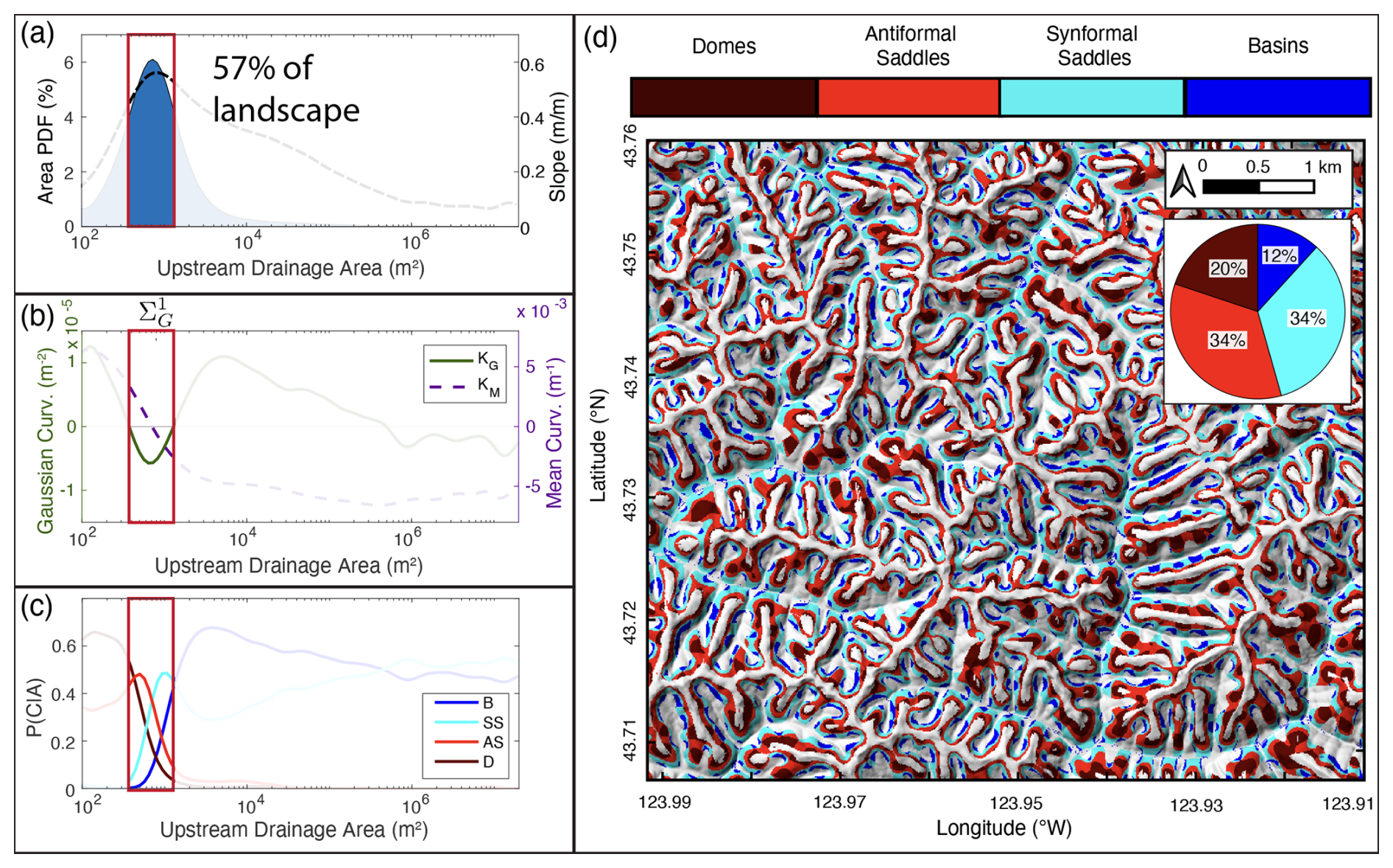
Figure 10 Surface geometry data for region ${\mathrm{\Sigma }}_{\mathrm{G}}^{\mathrm{1}}$: points in the landscape with upstream drainage areas between 3.75×10² and 1.29×10³ m². The red box in each of the area-binned plots (a–c) highlights the range of included drainage areas. (a) PDF of drainage areas. (b) Gaussian and mean curvatures binned by area. (c) Conditional PDFs of shape classes. (d) Map of shape classes projected on a focused subregion of the study area. Pie-chart inset shows shape-class composition of the surface.

5.1.3 ${\mathrm{\Sigma }}_{\mathrm{G}}^{\mathrm{2}}$: drainage areas between 1.29×10³ and 3.80×10⁵ m²

At drainage areas of 1.29×10³ m², the Gaussian curvature again changes sign, increasing to a local maximum at ∼ 4.50×10³ m² before steadily returning to zero at 3.30×10⁵ m² (Fig. 11b). We define our third landscape region (${\mathrm{\Sigma }}_{\mathrm{G}}^{\mathrm{3}}$) between these inflection points. Here, the convergence of surface gradient vectors is indicated by negative K_M and the dominance of basins (60 %) and synformal saddles (36 %). This geometry intuitively implies colluvial hollows, where unconsolidated material collects at the head of debris-flow networks (Dietrich et al., 1993). At drainage areas exceeding that of the local maximum in Gaussian curvature (Fig. 11b), the decrease in both K_G and K_M is consistent with increasing downstream channelization in debris-flow channels (Stock and Dietrich, 2003; McGuire et al., 2023). This same trend is apparent in the shape class distributions in Fig. 11c, where basins trade off with synformal saddles as surface gradient vectors converge. This region makes up 25 % of the study area.

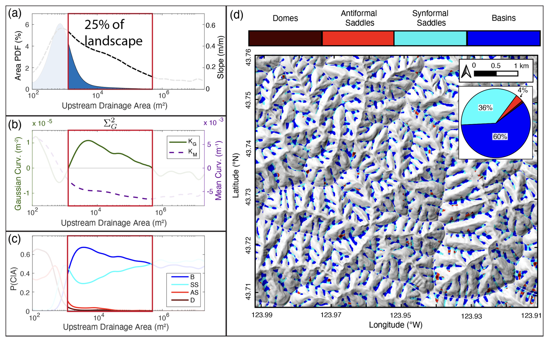
Figure 11 Surface geometry data for region ${\mathrm{\Sigma }}_{\mathrm{G}}^{\mathrm{2}}$: points in the landscape with upstream drainage areas between 1.29×10³ and 3.80×10⁵ m². The red box in each of the area plots highlights the region of interest. (a) PDF of drainage areas. (b) Gaussian and mean curvatures binned by area. (c) Conditional PDFs of shape classes. (d) Map of shape classes projected on a focused subregion of the study area. Pie-chart inset shows shape-class composition of the surface.

5.1.4 ${\mathrm{\Sigma }}_{\mathrm{G}}^{\mathrm{3}}$: drainage areas greater than 3.80×10⁵ m²

The last inflection point in Gaussian curvature occurs at drainage areas of 3.80×10⁵ m², where synformal saddles surpass basins as the dominant morphology (Fig. 12c). The growing influence of channels in defining landscape curvature is consistent with area-space fluvial transitions inferred elsewhere in the literature (Montgomery and Foufoula‐Georgiou, 1993). The spatial contribution of this region is extremely small (< 1 % of the land surface; Fig. 12a), with little geometric change across the two orders of magnitude spanned by drainage area. The only overall trend is a gradual decrease in the magnitude of mean curvature, which could indicate downstream valley widening as erosional efficiency increases. However, a close look at the map-view shape distribution (Fig. 12d) reveals regular transitions between basin and saddle structures, indicating along-channel oscillations in the first principal curvature (k₂ is always negative in a channel).

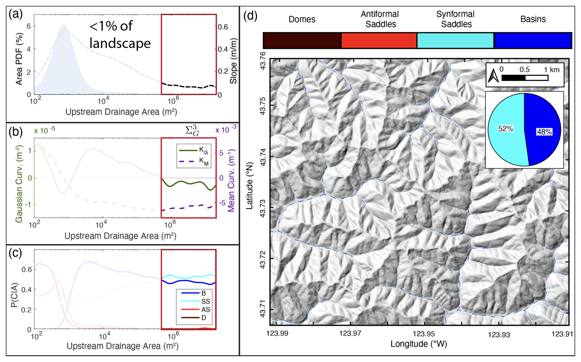
Figure 12 Surface geometry data for region ${\mathrm{\Sigma }}_{\mathrm{G}}^{\mathrm{3}}$: points in the landscape with upstream drainage areas greater than 3.80×10⁵ m². The red box in each of the area plots highlights the region of interest. (a) PDF of drainage areas. (b) Gaussian and mean curvatures binned by area. (c) Conditional PDFs of shape classes. (d) Map of shape classes projected on a focused subregion of the study area. Pie-chart inset shows shape-class composition of the surface.

5.2 Landscape partitioning from mean curvature

In this section we show that mean curvature also provides a way of understanding connections between geometry and process in fluvial topography. We decompose the landscape into two regions (${\mathrm{\Sigma }}_{\mathrm{M}}^{\mathrm{0}}$ and ${\mathrm{\Sigma }}_{\mathrm{M}}^{\mathrm{1}}$) separated by the single inflection in K_M at drainage areas of 7.40×10² m². Results are shown in Fig. 13. Alignment between this point in area-space and the peak of the slope curve in Fig. 13a is consistent with the idea that curvature decreases as hillslope profiles approach an angle-of-repose (∼ 30° inferred from the peak of the slope curve in Figs. 8–12), above which loose material is gravitationally unstable (Roering et al., 2007). Downhill of this point, slope decreases and unconsolidated material will tend to collect as colluvium at the head of the channel network (region ${\mathrm{\Sigma }}_{\mathrm{G}}^{\mathrm{2}}$).

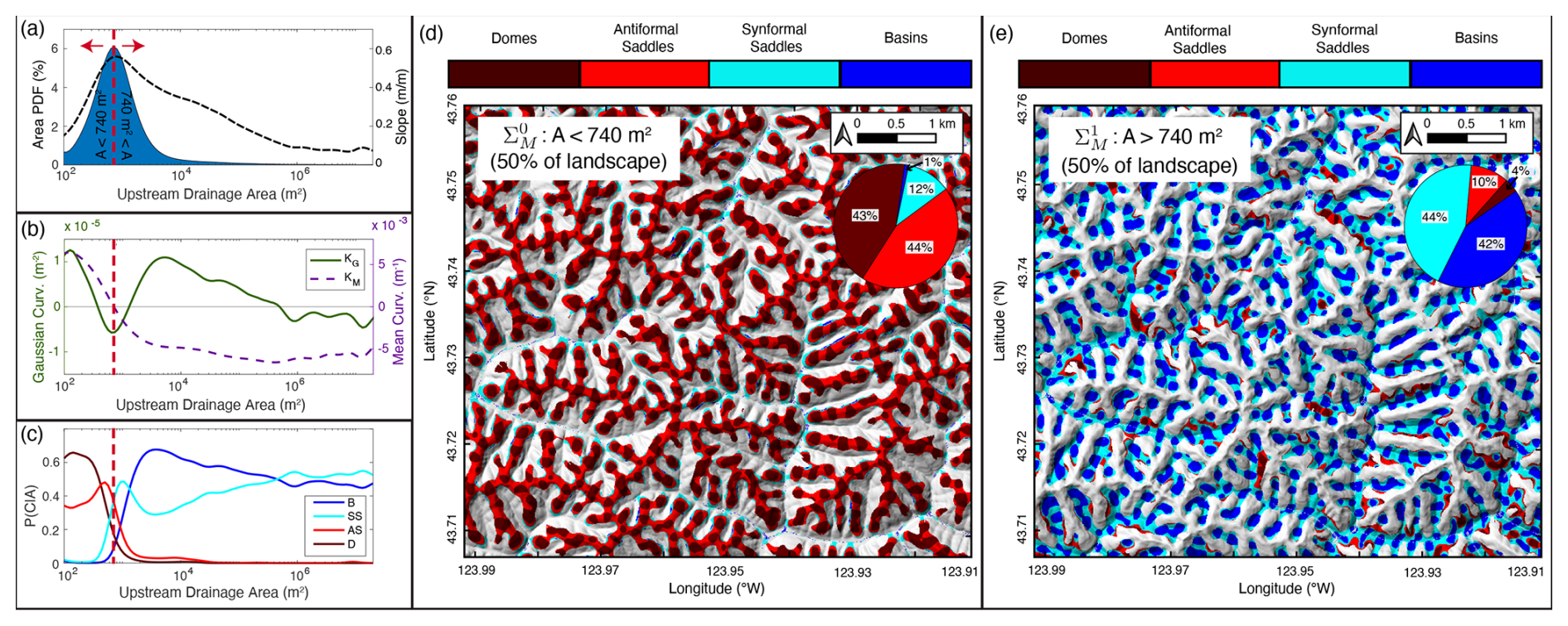
Figure 13 Maps of surface geometry for landscape partitioning about the mean curvature inflection point at drainage areas of 7.40×10² m². Red-dashed lined shows location of curvature inflection point. (a) PDF of drainage areas. (b) Gaussian and mean curvatures binned by area. (c) Conditional PDFs of shape classes. (d) Map of shape classes for drainage areas less than 7.40×10² m². (e) Map of shape classes for drainage areas greater than 7.40×10² m². Pie-chart insets on panels (d) and (e) show shape-class compositions of the surfaces.

Partitioning the landscape this way reveals surprising symmetries in both shape class distributions and surface geometry metrics for the two regions (Fig. 13d–e). The landscape is equally distributed about this zero crossing. For our filtering method and scale, 50 % of points are above or below the most probable drainage area value in our study area. Figure 14a shows a map of the study area divided into concave and convex domains based on this area threshold. Probability distributions of slope, mean curvature, and Gaussian curvature for the two regions are shown in Fig. 14b–d. While the slope and Gaussian curvature are similarly distributed in the concave and convex landscape regions, we see that the mean curvature has mirrored distributions such that the integrated mean curvature in the landscape is approximately zero.

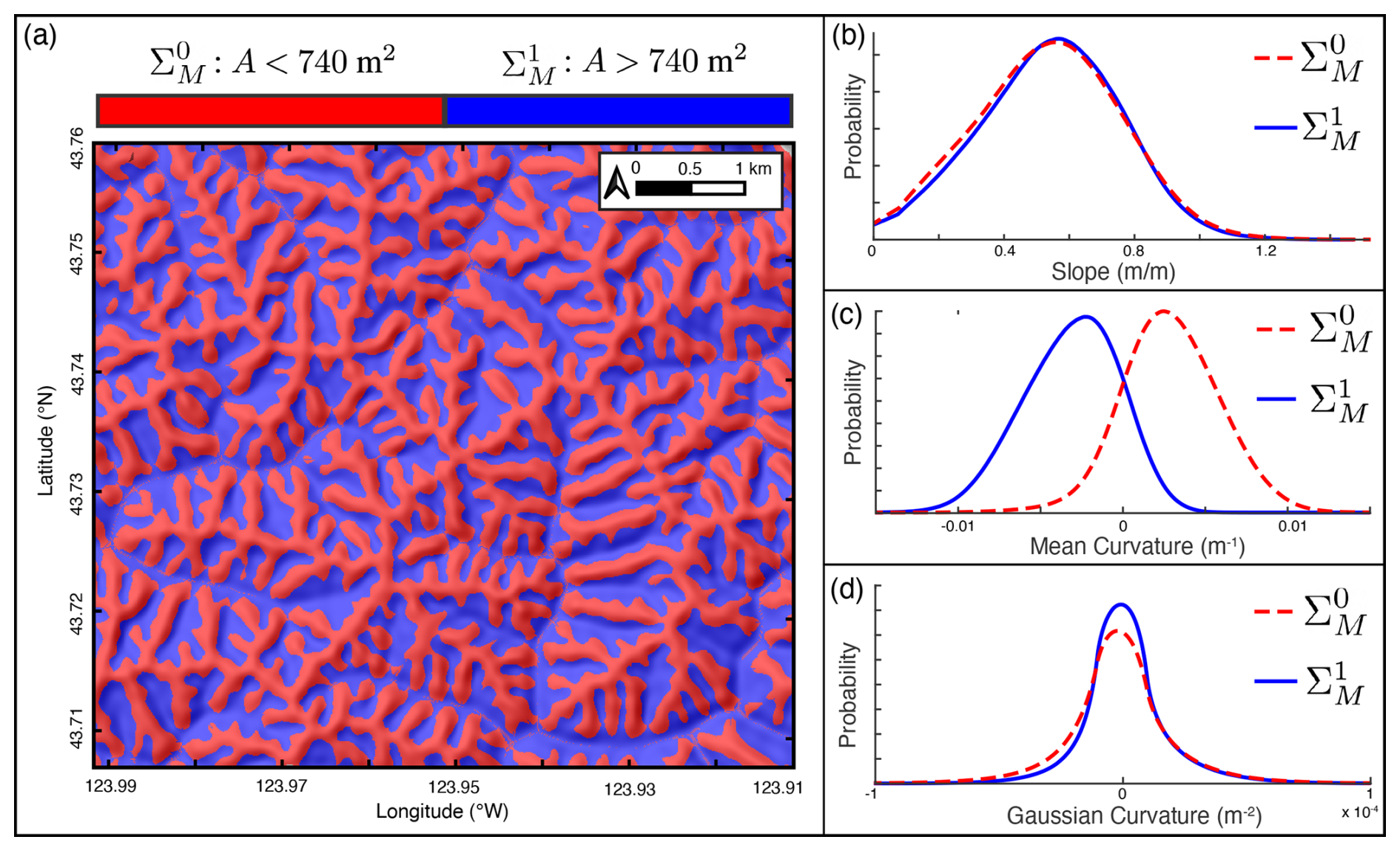
Figure 14 Distribution of surface geometry metrics for regions defined by the mean curvature inflection point. (a) Map-view of landscape partitioned about the point of inflection in K_M. (b) Distribution of tangent slope in regions of both negative and positive average K_M. (c) Distribution of mean curvature in regions of both negative and positive average K_M. (d) Distribution of Gaussian curvatures in regions of both negative and positive average K_M.

5.3 Geometric properties of channels and ridges

We have thus far focused on documenting Oregon Coast Range landscape segmentation in drainage area from a curvature perspective. A clear corollary to this is to ask specifically about the emergent channel and ridge network structures that manifest from this drainage area segmentation. It is well established that curvature provides a powerful tool for extracting continuous concave-up structures and deriving definitions of channel networks that are self-consistent throughout the landscape (Passalacqua et al., 2010; Gallant and Hutchinson, 2011; Bonetti et al., 2018). Our methods are suitable for this task as well, and for the parallel extraction of concave-down ridge network structures (Scherler and Schwanghart, 2020), but we will not pursue that objective here.

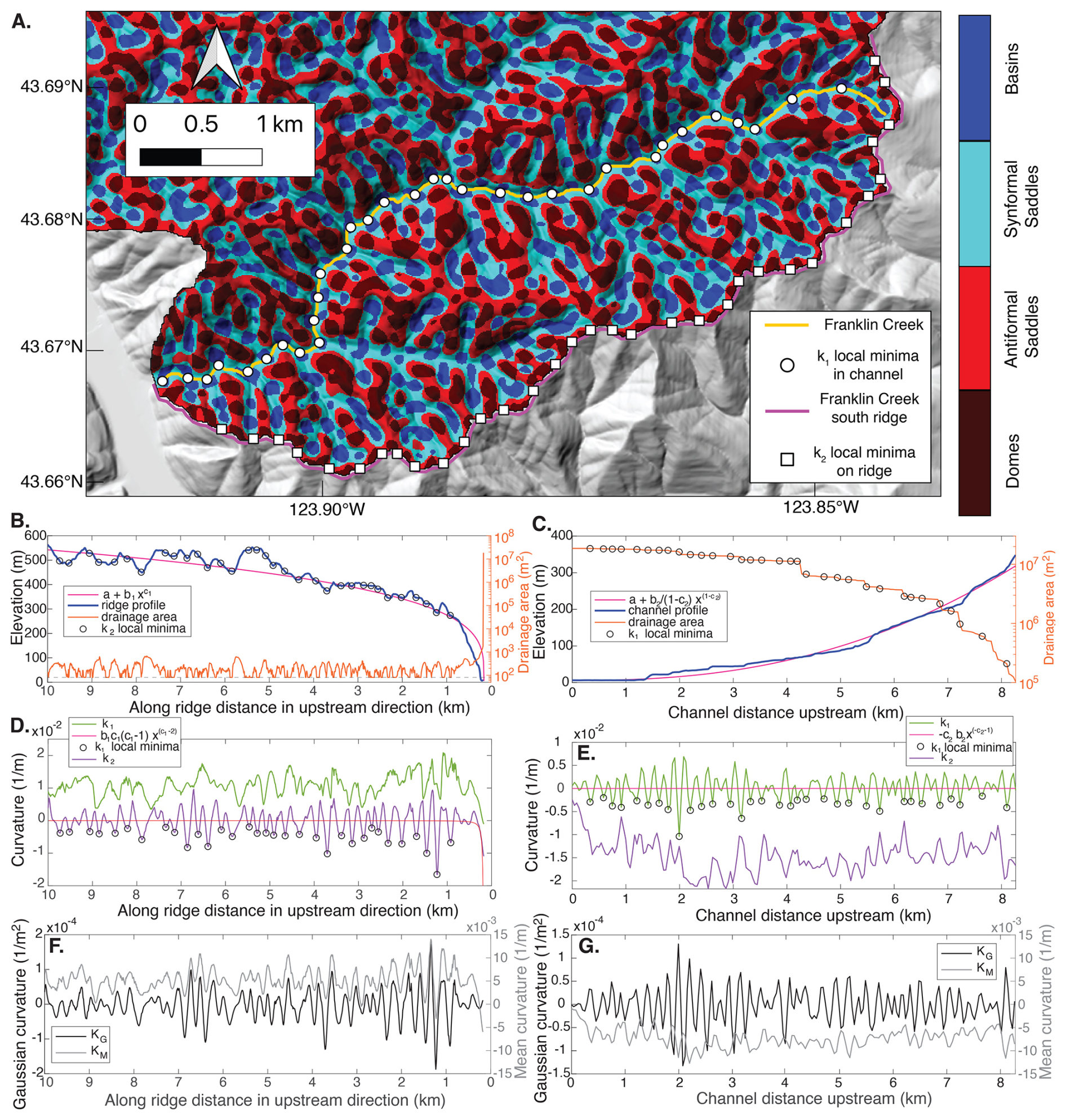
Figure 15 Characteristics of Franklin Creek and its south ridge. (A) Curvature shape classes with channel and ridge highlighted in yellow and magenta. Circles are local minima of along-channel principal curvature k₁ while squares are local minima of along-ridge principal curvature k₂. (B) Ridge elevation profile (left axis) and drainage area (right axis). Dashed line is drainage area for one cell. Pink curve is a powerlaw fit (fit parameters are listed in text). (C) Channel elevation profile (left axis) and drainage area (right axis). Pink curve is a powerlaw fit. (D) Principal curvatures along the south ridge. Note that local minima in k₂ (black circles) correspond to local saddles directly upslope from 1st order channel heads in panel (A). The mean of k₁=0.01 m⁻¹ and the mean of $k_{\mathrm{2}}=-\mathrm{3.49}\times {\mathrm{10}}^{-\mathrm{4}}$ m⁻¹. (E) Principal curvatures along Franklin Creek. Note that local minima in k₁ (black circles) correspond to junctions between tributary channels in panel (A). The mean of $k_{\mathrm{1}}=\mathrm{8.32}\times {\mathrm{10}}^{-\mathrm{5}}$ m⁻¹ and the mean of $k_{\mathrm{2}}=-\mathrm{0.01}$ m⁻¹. The red curve comes from stream power (it has a mean value of $\mathrm{1.10}\times {\mathrm{10}}^{-\mathrm{5}}$ m⁻¹). (F, G) Profiles of Gaussian curvature K_G and Mean curvature K_M along ridge and channel.

Instead, we will focus on the strikingly even partitioning of mean curvature between concave up structures (channels) and concave down structures (ridges). These structures are themselves composed entirely of alternating basins and synformal saddles (in channels) and domes and antiformal saddles (on ridges). Figure 15a shows a close-up of our study area around Franklin Creek to demonstrate this pattern. While the size distribution of these alternating shape classes within a channel or ridge is variably sensitive to lowpass filter threshold, the shape classes themselves are much more robust as they reflect zero crossings in K_M and K_G whose positions are insensitive to filter cutoff (Fig. 4), particularly in the case of mean curvature. This alternating pattern of local shape classes, originally recognized qualitatively by Cayley (1859) and Maxwell (1870), manifests clearly in channel and ridge network geometry.

Figure 15b–c plots in blue the elevation of Franklin Creek and its south ridge as a function of distance from the most downstream point of the creek (where it intersects the Umpqua river). The drainage area (red curves) along these structures (calculated using the intrinsic area calculation method in Sect. 4.3.3) reflects expectations: discontinuities in drainage area along the channel correspond to tributary junctions while ridge-top drainage area deviates from one grid cell only in saddles (up to 8 grid cells long here) between local maxima.

Figure 15d–e plots the signed principle curvatures for ridge and channel. An immediate comparison of note is that local minima in k₁ for the channel and k₂ for the ridge correspond to basins and antiformal saddles, respectively (circles). These structures align with tributary junctions in the channel, and lie directly upslope of 1st order channel heads on the ridge. This indicates that the curvature shape classes reflect structural changes in network geometry for both concave and convex topography. Neither structure – the local basins at channel junctions or saddles on ridgetops corresponding to transitions from hillslopes to channels – have been previously described to our knowledge. As these geometries describe changes in curvatures associated with branching structures in channels and ridges, their locations are minimally sensitive to the filter cutoff used for smoothing the DEM.

Figure 15f–g then plots the Gaussian (K_G) and mean (K_M) curvatures along the channel and ridge. The notable comparison in this case is that local maxima in K_G and K_M are anticorrelated along the channel and correlated along the ridge. This symmetry reflects the paired shape classes in either structure.

Comparing channel and ridge geometries we see that, in both cases, the two measures of curvature (principle curvatures or invariants) are near mirror-images of each other. One metric oscillates around zero (a principle curvature in Fig. 15d–e and K_G in Fig. 15f–g), while the other is strictly positive (for ridge) or negative (for channel), although still oscillatory. The along-channel and along-ridge envelope of this latter metric varies non-monotonically as expected for a small dendritic drainage basin, but also exhibits coincident channel widening (decrease in the magnitude of k₂) and ridge narrowing (increase in k₁ towards the mouth of Franklin Creek (distances ≲ 2300 m).

Finally, while the development of curvature-driven process models is outside the scope of this work, it is informative to compare the observed curvature of channel and ridge to theoretical models. Figure 15c–e show best fitting power laws to ridge and channel, after (Whipple and Tucker, 1999) for bedrock channel longitudinal profile and models such as those of Willett (2010) for interfluvial ridge elevations. The fit constants are a=6 m, $b_{\mathrm{1}}=\mathrm{2.84}\times {\mathrm{10}}^{-\mathrm{7}}$ m^−1.4, $c_{\mathrm{1}}=-\mathrm{1.4}$, b₂=41.88 m^0.72, c₂=0.28.

For Franklin Creek, while the elevation profile is well-approximated by a stream power-law fit, the resulting curvature (obtained by differentiating the longitudinal profile twice with respect to alongstream distance x) does not capture oscillations observed in k₁, the along-channel principal curvature. However, the average value of the stream power model curvature ($\mathrm{1.1}\times {\mathrm{10}}^{-\mathrm{5}}$ m⁻¹) is close to the average value of k₁ ($\mathrm{8.3}\times {\mathrm{10}}^{-\mathrm{5}}$ m⁻¹) extracted from the DEM (we expect an even closer match if tributaries are included in the stream power model, e.g., Willett, 2010). Thus, the steady state model approximates the average concavity of the true channel geometry, despite much larger curvature oscillations associated with local basin structures at tributary junctions.

Similarly, a power-law fit to the Franklin Creek south ridge profile in Fig. 15c well represents the elevation but fails to capture the smaller scale curvature oscillations oscillations between domes and antiformal saddles. The average value of this fit ($-\mathrm{3.3}\times {\mathrm{10}}^{-\mathrm{4}}$ m⁻¹) is within 7 % of the average value of k₂ ($-\mathrm{3.5}\times {\mathrm{10}}^{-\mathrm{4}}$ m⁻¹) extracted from the DEM, reflecting the overall concave down nature of the along-ridge curvature. These results suggest that standard fluvial process models, while missing physical ingredients at smaller scale, capture network-scale curvatures of channels and ridges.

6 Future directions

Quantitative classification of landforms and topography generally is challenged by the myriad interacting physical processes shaping landscapes at a range of spatial and temporal scales. Nevertheless, certain metrics such as local slope and drainage area have, through extensive empirical validation, proven to be useful indicators of spatial process transitions (Montgomery and Foufoula‐Georgiou, 1993; Rosenbloom and Anderson, 1994; Stock and Dietrich, 2003) and transient landscape evolution (Kirby and Whipple, 2012; Royden and Perron, 2013).

In our Coast Range study area curvature invariants – referenced to drainage area through ${\mathrm{\Sigma }}_{\mathrm{G}}^j$ and ${\mathrm{\Sigma }}_{\mathrm{M}}^j$ thresholds (Figs. 9–14) – separate the landscape into regimes that can be clearly associated with well known geomorphic processes. The ${\mathrm{\Sigma }}_{\mathrm{G}}^j$ and ${\mathrm{\Sigma }}_{\mathrm{M}}^j$ are separated by area-space inflection points (zero crossings) in Gaussian and mean curvature and appear to be minimally sensitive to DEM quality or smoothing. We expect that the ${\mathrm{\Sigma }}_i^j$ regimes, reflecting areas dominated by different combinations of convex and concave shape classes, should occur in all landscapes because they encode a distribution of “critical points” that characterize stability and continuity in all 2D surfaces (Matsumoto, 2001). These geometries have implications for the sensitivity of landforms to external perturbation. In steady-state landscapes, diffusive processes are expected to localize in locations of high curvature (Anand et al., 2023) consistent with the curvature distributions observed here. We therefore hypothesize that variation in drainage area values associated with ${\mathrm{\Sigma }}_i^j$ domains – perhaps in particular the concavity transition between ${\mathrm{\Sigma }}_{\mathrm{M}}^{\mathrm{0}}$ and ${\mathrm{\Sigma }}_{\mathrm{M}}^{\mathrm{1}}$ – may reflect signatures of landscape disequilibrium, as perturbations to steady-state would be expected to effect the geometry of these high-curvature regions.

More broadly, the presence of persistent curvature patterns in channel and ridge networks suggest the potential for new insights into geomorphic processes. For example, while the magnitude of curvature oscillations in Fig. 15 need to be validated by field studies, the ability to potentially detect step-pool morphology at the landscape scale could open the door to connecting localized models of mass transport in rivers to landscape scale erosion models applied to topographic datasets (Venditti et al., 2020; Church and Zimmermann, 2007; Scheingross and Lamb, 2017; González et al., 2017; Escauriaza et al., 2023). In addition, the discernible valley widening signal discussed in Sect. 5.3 could aid understanding of known correlations between valley width and other landscape parameters (Bernard et al., 2022; Turowski et al., 2024).

Similarly, the ability to robustly identify colluvial hollows (a prominent component of ${\mathrm{\Sigma }}_{\mathrm{G}}^{\mathrm{2}}$), where the topographic surface is shaped by a superposition of competing processes at the onset of convergent topography (Dietrich et al., 1993), demonstrates the utility of this approach. In landscape regions shaped by debris flow processes (Iverson and George, 2024), strongly disequilibrium dynamics (Donahue et al., 2013; Klema et al., 2023), glacial erosion (Kober et al., 2019), or even those dominated by constructional landforms such as in volcanic terrane (Karlstrom et al., 2025), slope-area scaling and other commonly used process-oriented classification approaches break down and tools such as developed here are likely to be useful. Because surface curvature also influences shallow subsurface stress state for rock fracture (Martel, 2011; Clair et al., 2015; Moon et al., 2017) and the hydraulic gradients driving groundwater flow (Wörman et al., 2006; Zhang et al., 2022), we expect that problems in Critical Zone science may also be examined through the lens of topographic curvature (Riebe et al., 2017).

Many processes driving landscape evolution have an intrinsic scale length (Wegmann et al., 2007; Crozier et al., 2018; Roering et al., 2010), so the combination of spectral filtering to isolate certain topographic features with curvature analysis seems a promising direction for future efforts in complex geomorphic settings (Perron et al., 2008). For example, 1-D measures of hillslope length in the Oregon Coast Range (Grieve et al., 2016; Roering et al., 2007) could be compared to average path lengths in the ${\mathrm{\Sigma }}_{\mathrm{G}}^{\mathrm{1}}$ region to quantify similarities between intrinsic and extrinsic approaches, with a physically justified definition of the domain boundary given by our partitioning scheme. Quantitative comparison of our results with such studies of isolated landscape domains is a clear next step in the development of these methods.

From a practical standpoint, Fig. 6f highlights how intrinsic geometric computation of topographic metrics such as slope, curvature, and drainage area differ from the standard approach using an extrinsic map view projection of a DEM. The ${\mathrm{\Sigma }}_i^j$ regimes (e.g., as illustrated on Fig. 8b) appear to be relevant. For example, curvature and drainage area computed over ${\mathrm{\Sigma }}_{\mathrm{G}}^{\mathrm{1}}$, encompassing steep hillslopes, exhibit average differences of ∼ 50 % and ∼ 15 % respectively, which are larger than any other segment of the landscape. Slopes computed in either ${\mathrm{\Sigma }}_{\mathrm{G}}^{\mathrm{0}}$ or ${\mathrm{\Sigma }}_{\mathrm{G}}^{\mathrm{3}}$, representing the smallest and largest drainage areas, are maximally different by ∼ 30 %. Because the ${\mathrm{\Sigma }}_{\mathrm{G}}^{\mathrm{1}}$ region accounts for the majority of land surface area (Fig. 10a), differences in drainage area from ${\mathrm{\Sigma }}_{\mathrm{G}}^{\mathrm{1}}$ persist across all higher drainage areas with average values ∼ 10 %. Understanding the effects of projection distortion on empirical scaling relations (e.g., Hack's Law, Hack et al., 1957, relies on drainage area computed from a DEM), and process-based models (e.g., sediment mass-continuity and stream power; Whipple and Tucker, 1999), will likely be a fruitful direction for future work.

In general, we see potential for this approach applied to high-resolution LiDAR or structure-from-motion data, where signatures of processes at many scales of associated curvature variations can be resolved. For example, hillslope processes are sensitive to bioturbation (Gabet, 2003) and tree throw (Roering et al., 2010), signatures of which cannot be resolved in the dataset used here. In steep channels, this approach could be useful in defining the geometry of complex features such as waterfall plunge pools (Scheingross and Lamb, 2017) and disentangling the processes governing rock fracture and cliff erosion (DiBiase et al., 2018; Martel, 2011).

7 Conclusions

Building on Gauss's classical results in intrinsic surface characterization, we derive topographic geometry metrics for landform characterization and landscape segmentation on discretely sampled surfaces. We show that digital elevation models of topography, after appropriate smoothing, can be categorized point-wise as one of four surface shape classes that provide a natural means of landscape segmentation that highlights channels, basins, domes, and saddles (28 %, 22 %, 23 %, and 27 % of the landscape respectively). An application to the Oregon Coast Range shows that the distribution of curvature invariants reveals details about the geometric evolution of fluvial systems. We partition the area-space landscape into four domains based on the sign of the Gaussian curvature (${\mathrm{\Sigma }}_{\mathrm{G}}^{\mathrm{0}}-{\mathrm{\Sigma }}_{\mathrm{G}}^{\mathrm{3}}$), and show how these partitions correspond to previously identified geomorphic process domains. Mapping mean curvature over the entire landscape reveals a remarkable symmetry that is reflected in total landscape curvature and slope distributions, and in the profile curvatures measured along ridge/channel networks. We hypothesize that such symmetry reflects a signature of steady-state fluvial topography. Lastly, we show that oscillations in curvatures perpendicular to channels and ridges are expressed in a regular geometric pattern that capture geometric transitions between concave and convex topographic forms.