Challenges in reconstructing seasonally driven landslide motion from optical satellite data: insights from the Del Medio catchment, NW Argentina

Optical satellite images are a valuable resource for studying slow-moving landslides from space. However, monitoring displacement through pairwise image correlation and time-series inversion presents several challenges, including the impact of seasonality on measurement accuracy. Seasonal biases arise from systematic measurement errors related to variable illumination conditions and shadows. These errors manifest in the form of an oscillation pattern in the satellite-derived time series. This complicates the identification of any true seasonal component linked to feedback mechanisms between landslide displacement and a seasonally variable climate.

Here, we provide a comprehensive evaluation of different strategies to reduce the magnitude of seasonal biases. These include modeling the seasonal error component, restricting correlation to pairs with similar illumination, weighting, and upsampling optical images. We find that all methods can reduce the impact of systematic seasonal bias with different trade-offs: longer processing times, creation of sparse or disconnected networks, dependence on topographic data, or potential alteration of the true displacement signal.

We evaluated the removal of seasonal bias from displacement time series derived from optical satellite data (Landsat-8, Sentinel-2, PlanetScope) over a large slow-moving landslide in the Río Del Medio catchment in northwest Argentina. The transition zone between the Altiplano-Puna plateau and the Andean foreland is characterized by a highly seasonal climate, with intense rainfall during the South American summer monsoon and semi-arid conditions throughout the rest of the year. Over the 10-year observation period, the landslide accumulated approximately 35 m of displacement at spatially and temporally variable rates. After the removal of the seasonal bias component, we observe several acceleration phases, which all fall within the rainy season of the respective year. The timing of the acceleration suggests precipitation as a major driver of a landslide that is already preconditioned by infiltration and sliding through inherited fault structures, weakened lithologies, and freeze-thaw processes at high altitudes of up to 4500 m above sea level.

Based on this example, our study provides a basis for selecting the appropriate correction methods to address seasonal biases. Considering all effects of seasonality is essential to improve the accuracy of satellite-derived displacement measurements and better constrain the feedback mechanisms between landslide velocity and a seasonal climate.

1 Introduction

Slow-moving landslides are a common phenomenon in mountainous regions, where they pose threats to local infrastructure, alter sediment-transport patterns, may fail catastrophically, and ultimately lead to cascading effects downstream (e.g., Handwerger et al., 2013; Lacroix et al., 2018; Handwerger et al., 2019a; Lacroix et al., 2020; Van Wyk de Vries et al., 2022). Given their hazard potential, there is an interest in detecting and monitoring unstable slopes. For landslides moving at rates of 1–100 m yr⁻¹, cross-correlation of optical satellite imagery is a viable and cost-effective method for measuring surface displacement, especially in steep and inaccessible terrain. Displacement time series from optical data are traditionally obtained through pairwise correlation of images acquired at different points in time, thereby establishing a redundant network of displacement maps. Subsequently, a displacement signal can be reconstructed from the temporally overlapping measurements by solving a matrix system through time-series inversion (e.g., Bontemps et al., 2018; Lacroix et al., 2019; Ding et al., 2021; Dille et al., 2021; Provost et al., 2022) – an approach adapted from the time-series analysis of Interferometric Synthetic Aperture Radar (InSAR) data (Berardino et al., 2002; Doin et al., 2011). The derived time series is the basis for subsequent interpretations of the landslide's behavior, making it essential to obtain reliable results from this step. However, displacement measurements obtained from satellite images can be biased due to several reasons, including image distortions, limited co-registration accuracy, orthorectification errors, algorithmic errors, shadows, land cover changes, and seasonal variations of illumination, humidity, and vegetation (e.g., Leprince et al., 2007; Scherler et al., 2008; Stumpf et al., 2014; Lacroix et al., 2019; Mueting and Bookhagen, 2024; Antoine and Liu, 2025).

Some of these errors are correlated in time. In particular, illumination changes and shadow effects pose a challenge in reconstructing landslide motion. When images from different seasons are correlated, variable illumination and shadows can lead to systematic measurement errors. Seasonal biases in pairwise displacement measurements result in an oscillation pattern in the time series obtained through temporal inversion (Lacroix et al., 2019). When seasonal biases mix with the landslide displacement signal, oscillations may be misinterpreted as or obscure an existing relationship between landslide motion and seasonally changing environmental conditions – slow-moving landslides are known to respond to changes in porewater pressure induced by rainfall or snow melt (Hilley et al., 2004; Handwerger et al., 2013). Mitigating the impact of seasonal biases is therefore essential to correctly interpret satellite-derived displacement estimates.

Previous studies have taken different approaches to reduce the effect of variable illumination and shadows, including modeling seasonal oscillations on static terrain with exposition similar to the landslide through harmonic functions (Lacroix et al., 2019), masking shadows before correlation (Provost et al., 2022), or restricting correlation to image pairs acquired under similar illumination conditions (Dehecq et al., 2015; Hollingsworth et al., 2017; Ding et al., 2020, 2021). However, there is no consensus yet on which approach is best suited to address seasonal biases in time series retrieved from optical image matching.

In this study, we examine different mitigation strategies and assess their advantages and limitations. In addition, we compare measurements from PlanetScope, Sentinel-2, and Landsat-8 imagery to assess seasonal measurement biases in displacement estimates from different sensors at different spatial resolutions. As a test case scenario, we chose a large, slow-moving landslide located in the Río Del Medio catchment, within the Quebrada del Humahuaca in northwest Argentina, as well as synthetic examples. Through the careful evaluation of seasonal biases, we aim to (1) achieve the best possible reconstruction of the displacement history of the last 10 years in the Río Del Medio catchment area, (2) determine if and how a potential real seasonal displacement signal can be decoupled from measurement errors, and (3) provide a basis for selecting a suitable correction approach considering local conditions, data availability, and processing capabilities.

2 Study area

Our analysis focuses on a slow-moving landslide located in the catchment of the Río (or Arroyo) Del Medio, which we subsequently refer to as the Del Medio landslide. The Río Del Medio is a tributary of the Río Grande, draining the intermontane Humahuaca Basin in the Eastern Cordillera of northwest Argentina. The landslide is situated on the steep slopes of the eastern drainage divide of the Del Medio catchment with peaks that reach 4500 m above sea level (Fig. 1a). Due to the eastward dip of the landslide slope, we primarily consider the east-west component of displacement in this study. The Del Medio basin is bounded by two north-south striking faults, both of which are inherited normal faults that have been inverted under a compressional regime (Rodríguez Fernández et al., 1999). The exposed lithologies include the pervasively sheared phyllites of the Puncoviscana Formation and the quartzitic rocks of the Mesón group in the upper part of the catchment (Savi et al., 2016; Rodríguez Fernández et al., 1999). The vegetation cover at these altitudes is sparse and dominated by shrubs and grassland steppe (Angillieri et al., 2020). Notable is the scar and deposits of a catastrophic rockfall event that occurred during the rainy season of 2009 (Fig. 1b–c), which caused several tens of meters of elevation changes (Purinton and Bookhagen, 2018). Recent research showed that the landslide is still active: downhill movement with rates between 2–5 m yr⁻¹ was detected for the years 2020–2023 in the area of the 2009 failure (Mueting and Bookhagen, 2024). Using satellite imagery from multiple sources, this study extends displacement monitoring to the time period between 2014 and 2024.

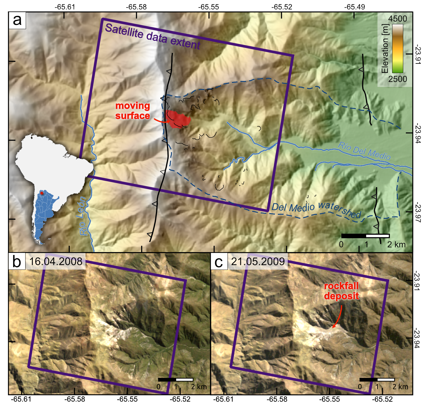
Figure 1 (a) Colorized shaded relief map of the Del Medio catchment in the Quebrada del Humahuaca based on the Copernicus DEM at 30 m resolution (European Space Agency, 2024). Scarps of historical landslide events are indicated as black lines and geologic structures (inverted normal faults) (Rodríguez Fernández et al., 1999) as black lines with tick marks. The surface of the actively moving block is highlighted in red. The area of interest to which all satellite data was cropped is shown in purple. Panels (b) and (c) depict two cloud-free Landsat-5 images (Earth Resources Observation and Science (EROS) Center, 2020) with similar illumination conditions before and after the major rockfall event that occurred at the Del Medio landslide during the rainy season in 2009. Additional Landsat-5 acquisitions with partial cloud cover constrain the timing of the rockfall between 13 January and 2 March 2009.

Landslides and rockfalls in the Del Medio catchment provide large amounts of material that is transported by debris flows and deposited in an actively aggrading fan (Savi et al., 2016). Debris flows sourced from the Del Medio and adjacent catchments typically occur during the austral summer monsoon when heavy rainfall can mobilize loose material and transport it downstream (Savi et al., 2016; Angillieri et al., 2020). This high seasonality observed in the sediment transport processes raises the question of whether landslide displacement rates in the Del Medio catchment are also driven by high precipitation rates during the rainy season – a question this study tries to answer based on displacement time series inferred from optical satellite data.

3 Materials and Methods

3.1 Satellite data

Offset tracking was performed using cloud-free optical satellite imagery from Landsat-8 (43 images), Sentinel-2 (41 images), and PlanetScope (87 images). The archive of the PlanetScope constellation consists of data captured by different instrument generations. We used imagery acquired by the PSB.SD instrument (SuperDove) in orbit since March 2020, and the older PS2 (Dove-C) generation with the earliest available imagery over the Del Medio landslide from mid-2016. Taken together, all satellites provide insights into the displacement history of the Del Medio landslide since 2014 and allow a comparison for a common timespan from 2017 to 2024. Imagery was chosen based on cloud- and snow-free conditions, similar viewing geometry in the case of PlanetScope, and full area of interest (AOI) coverage. For the PlanetScope PS2 instrument, where the comparably small scene sizes of 24 × 8 km did not always include the entire study area, scenes with slightly less coverage were also accepted. During the dry season, when many suitable scenes are available, imagery was randomly selected every one to two months to reduce computational load. For Landsat-8, we worked with the panchromatic band because of its highest spatial resolution (15 m). For Sentinel-2 and PlanetScope, we isolated the green band. The use of other bands (blue, red, infrared) from Sentinel-2 was shown to provide similar results (Lacroix et al., 2018). Combining multiple bands is not advised to avoid effects from interband misalignment issues, which were observed in PlanetScope scenes (Aati et al., 2022). All Landsat-8 scenes used in this study belong to the Collection 2, Tier 1, Level-1 dataset provided by the USGS. Sentinel-2 data were downloaded as Level 1C (geo- and radiometrically corrected) from the Copernicus Data Space Ecosystem. We selected Sentinel-2B to have data from a single satellite only, and also ensured that the images were processed with a baseline that used the Copernicus DEM for orthorectification. Geo- and radiometrically corrected PlanetScope data (Level-3B) were obtained through Planet's Education and Research program (Planet Team, 2025). Acquisition dates for the newer PSB.SD images align with the imagery used by Mueting and Bookhagen (2024), but all scenes were downloaded again to ensure a common processing baseline, because we observed that the reference DEM used during orthorectification has likely changed since the last data access (see Fig. S1 in the Supplement). We also added PS2 scenes, as well as additional PSB.SD acquisitions to extend and densify the correlation network.

A list of all scenes used in this work can be found in the Supplement (Tables S1 to S4). Sun elevation and azimuth angle of the scenes are plotted in Fig. S2.

3.2 Image correlation

Image correlation was carried out using Ames Stereo Pipeline (Beyer et al., 2018) for same-sensor image pairs. To ensure true comparability between the displacement fields obtained from satellite imagery at different native resolutions, we upsampled both Landsat-8 and Sentinel-2 to the 3 m spatial resolution of PlanetScope using cubic interpolation. Parameters were set to conform with Mueting and Bookhagen (2024): block matching with a correlation kernel of 35 × 35 pixels and subpixel refinement using an affine adaptive window with Bayes expectation-maximization weighting. We initially experimented with keeping the original resolution of the input imagery and adjusting the correlation kernel size in pixels to be constant in the area covered, but found a link between spatial resolution and magnitude of seasonal errors (see Sect. 4.3). To avoid the computational load of correlating all possible image pairs for every sensor, we employed a dynamic thresholding technique to identify suitable correlation pairs. We first obtained a rough estimate of the expected landslide displacement rates using Landsat-8 as the longest time series and correlating all image pairs with an arbitrary fixed threshold of a half-year minimum time difference. The resulting displacement time series was then used to approximate the displacement that accumulated during the time covered. If this number was above the detection threshold, assumed to be $\mathrm{1}/\mathrm{10}$ of the native pixel resolution, the image pair was considered in subsequent analyses. This dynamic pairing strategy results in many connections in phases of rapid movement and reduces the number of correlation pairs in years with no or very little displacement. As the land cover in the Del Medio catchment did not change much, we did not consider a maximum temporal threshold for the selection of image pairs. However, in areas with dense vegetation and anthropogenic land use, evolving land cover and a resulting decay in coherence is an additional factor that has to be taken into account.

For PlanetScope data, we added a constraint for the satellite viewing angle and only formed pairs among images with a common perspective (max ±0.6° view angle difference) to mitigate the effect of orthorectification errors (Mueting and Bookhagen, 2024). Also, PSB.SD and PS2 data were correlated separately due to the different instruments. Mixing images from different sources could be possible, but would introduce further complications due to different sensor specifications, acquisition geometries, and processing pipelines. Such an approach would make it more difficult to isolate and assess the effect of seasonal illumination changes. Overall, the pairing strategy resulted in 785 (Landsat-8), 752 (Sentinel-2), 271 (PlanetScope PSB.SD), and 220 (PlanetScope PS2) correlation pairs. See Figs. S3–S5 for a representation of all networks.

3.3 Post-processing

For Landsat-8 and Sentinel-2, we applied a median shift following image correlation to account for global shifts between reference and secondary image pairs. Median values were calculated with the landslide pixels masked out, assuming that the surrounding terrain remained stable. For PlanetScope, which is often affected by more complex co-registration error patterns, we modeled and removed global shifts, ramp, and orthorectification errors through a second-order polynomial fit, considering X and Y positions, as well as local elevation in the form of an external reference DEM (Mueting and Bookhagen, 2024).

3.4 Time-series inversion

Coherent time series were retrieved through an inversion based on the temporal closure of displacement measurement networks. The following system of linear equations is solved:

$$\begin{array}{}\text{(1)}& \mathbf{A}\mathit{X}=\mathit{B}\end{array}$$

where B is the vector storing all available displacement measurements obtained by the correlation of image pairs, A is the design matrix, and X denotes the vector containing the displacement estimates at each date. The design matrix A contains the values 0 and 1. 1 is assigned to each time step contained within the interval defined by the reference and secondary dates of acquisition of the image pair, and 0 elsewhere. This framework, known as the Leap Frog approach (Hadhri et al., 2019; Charrier et al., 2022b, c), solves for displacement at each time step, which is then added cumulatively to produce the final time series. For a connected network, the design matrix A is of full rank ($\mathrm{rank}\left(\mathbf{A}\right)=min(m,n)$ with m being the number of correlation pairs (rows in A) and n the acquisition dates (columns in A)). The system can be solved using an ordinary least-squares approach, which minimizes the sum of squared residuals:

$$\begin{array}{}\text{(2)}& \arg \min \left(\Vert \mathbf{A}\mathit{X}-\mathit{B}{\Vert }^{\mathrm{2}}\right)\end{array}$$

Optionally, weights can be added to the matrix system to favor displacement measurements that are less affected by errors. To add weights, both the design matrix A and the displacement measured through pairwise image correlation (vector B) are multiplied by a vector W containing the weights assigned to each displacement measurement:

$$\begin{array}{}\text{(3)}& \mathit{W}\mathbf{A}\mathit{X}=\mathit{W}\mathit{B}\end{array}$$

The inversion was carried out separately for each satellite to allow a comparison between the three data sources. Only for PlanetScope, we jointly inverted PSB.SD and PS2 correlation pairs. Due to the different instrument generations and grouping strategy based on common view angle, the PlanetScope network is disconnected, but with temporal overlap between groups. If not all dates within a network are connected through correlation, the matrix system (Eq. 1) becomes rank deficient ($\mathrm{rank}\left(\mathbf{A}\right)<min(m,n)$) and, as a consequence, the inversion problem becomes ill-posed. In this case, we include a first-order Tikhonov regularization term, as proposed by Bontemps et al. (2018) and Charrier et al. (2022b, c, a), which adds a penalty or regularization term as an additional minimization constraint to the least squares problem:

$$\begin{array}{}\text{(4)}& \arg \min \left(\Vert \mathbf{A}\mathit{X}-\mathit{B}{\Vert }^{\mathrm{2}}+\Vert \mathbf{\Gamma }\mathit{X}{\Vert }^{\mathrm{2}}\right)\end{array}$$

Here, Γ represents the regularization matrix, which is of size $n-\mathrm{1}\times n$. The matrix is filled with zeros, except for the diagonal, which is assigned the values $-\frac{\mathrm{1}}{\mathrm{\Delta }{\mathit{\tau }}_i}$ and the above element, which is set to $\frac{\mathrm{1}}{\mathrm{\Delta }{\mathit{\tau }}_i}$ (Charrier et al., 2022b):

$$\begin{array}{}\text{(5)}& \begin{array}{rl}& \mathbf{\Gamma }=\\ & \left[\begin{array}{ccccc}-\frac{\mathrm{1}}{\mathrm{\Delta }{{\mathit{\tau }}_i}_{d_{\mathrm{0},\mathrm{1}}}}& \frac{\mathrm{1}}{\mathrm{\Delta }{{\mathit{\tau }}_i}_{d_{\mathrm{1},\mathrm{2}}}}& \mathrm{0}& \mathrm{\dots }& \mathrm{0}\\ \mathrm{0}& -\frac{\mathrm{1}}{\mathrm{\Delta }{{\mathit{\tau }}_i}_{d_{\mathrm{1},\mathrm{2}}}}& \frac{\mathrm{1}}{\mathrm{\Delta }{{\mathit{\tau }}_i}_{d_{\mathrm{2},\mathrm{3}}}}& & \mathrm{0}\\ \mathrm{⋮}& & & \mathrm{\ddots }& \mathrm{0}\\ \mathrm{0}& \mathrm{0}& \mathrm{0}& -\frac{\mathrm{1}}{\mathrm{\Delta }{{\mathit{\tau }}_i}_{d_{n-\mathrm{2},n-\mathrm{1}}}}& \frac{\mathrm{1}}{\mathrm{\Delta }{{\mathit{\tau }}_i}_{d_{n-\mathrm{1},n}}}\end{array}\right]\end{array}\end{array}$$

Δτ_i corresponds to the temporal difference between each subsequent acquisition date. Including weights, the analytical solution of the matrix system, with the regularization term, can be formulated as:

$$\begin{array}{}\text{(6)}& \widehat{\mathit{X}}={\left({\mathbf{A}}^T\mathit{W}\mathbf{A}+\mathit{\lambda }{\mathbf{\Gamma }}^T\mathbf{\Gamma }\right)}^{-\mathrm{1}}{\mathbf{A}}^T\mathit{W}\mathit{B}\end{array}$$

The regularization parameter λ is a scaling constant with a default value of 1. The system, including the regularization term, is solved using a least squares solver for each pixel and for each component separately. This results in a multi-band raster that stores the cumulated displacement for each time step. The landslide surface was outlined through thresholding the maximum displacement field in combination with some manual adjustments based on photo interpretation. To avoid the impact of border effects at the transition between stable and moving terrain, we applied an inward buffer of half the correlation kernel size to the landslide outline, which concluded the final mask. The time series of the Del Medio landslide was generated by extracting all pixels inside this mask and calculating the mean and standard deviation.

3.5 Estimation of seasonal biases

Seasonal biases in pairwise displacement measurements typically manifest in the form of a regular seasonal oscillation pattern in the inverted time series. To estimate the magnitude of this signal, we model the seasonal bias component through a sine fit. First, we remove any nonlinear inter-annual displacement trend to keep the seasonal signal only. The trend is estimated using a rolling mean with a kernel of 13 months, as suggested by Lacroix et al. (2019). Then, we fit a sine wave with a fixed frequency of one year to the detrended signal:

$$\begin{array}{}\text{(7)}& y\left(t\right)=A\sin (\mathrm{2}\mathit{\pi }ft+\mathit{\varphi })+C\end{array}$$

where y is the cumulative displacement signal, A the amplitude, f the frequency, which is set to a fixed value of $\frac{\mathrm{1}}{\mathrm{365.25}}$, t the time in days, ϕ the phase shift, and C a constant that allows for vertical shift, in case the trend removal did not fully center the time series at zero. The amplitude of this sine wave is used in the following to quantify the effect of illumination changes on time-series inversion.

3.6 Mitigation of seasonal biases

In addition to estimating the magnitude of seasonal biases, we explore four different mitigation strategies.

3.6.1 Modeling of seasonal biases

A first strategy is to remove seasonal oscillations from the displacement time series using a harmonic function. In a previous study, Lacroix et al. (2019) considered the average sine fit over stable pixels with slope and aspect similar to the landslide to estimate and remove the seasonal bias component. We tried to replicate this approach for our study area by creating unique groups with common slope and aspect (5° bins). For each group, we calculated the median displacement time series excluding the landslide pixels and modeled the oscillations through a fixed-frequency sine function as described in Sect. 3.5. The resulting fit was subtracted from the displacement time series of all pixels with a common slope and aspect.

A second alternative strategy that relies on no external reference layer for the terrain attributes is the estimation and removal of the best-fit sine from the displacement time series of each pixel. This implies that regular seasonal oscillations are removed, irrespective of whether a pixel is located over the landslide or on stable ground. For moving ground, this method does risk the partial removal of true seasonal responses, which is further discussed in Sect. 4.4.

3.6.2 Pairing based on similar illumination

A third strategy aims at avoiding seasonal biases, rather than correcting their effects. Measurement noise has been shown to increase for correlation pairs acquired during different seasons (Bontemps et al., 2018; Mueting and Bookhagen, 2024) (Fig. 4). Consequently, image pairs with similar illumination conditions will be least affected by seasonal biases and should therefore be the most reliable basis for reconstructing a displacement signal. Several studies have restricted image correlation to similarly illuminated scenes to reduce seasonal biases (Dehecq et al., 2015; Hollingsworth et al., 2017; Ding et al., 2020, 2021). However, a major difficulty is the selection of a suitable tolerance threshold for the difference in illumination. Ding et al. (2020) determined suitable thresholds for the sun elevation and azimuth difference, as well as spatial and temporal baselines, through an iterative pairing process. Thresholds were defined to reduce differences in sun position while retaining enough image pairs to ensure a stable time-series inversion. Because narrow thresholds can split a network into several disconnected groups, a regularization term should be introduced to the inversion (see Eq. 4). When the network structure is already constrained, e.g., to the same viewing geometry for PlanetScope data, or simply by the number of available scenes, the threshold must be further loosened or even disregarded (Ding et al., 2021). To find an appropriate threshold for the data used in this work, we iteratively carried out the inversion over the Del Medio landslide using different sun azimuth and elevation thresholds for the pairwise measurements. We refined the sun positions provided in the scenes' metadata by calculating the sun elevation and azimuth angle for the latitude and longitude of the Del Medio landslide at the given acquisition time (Anderson et al., 2023). For every threshold, we estimated the seasonal oscillation amplitude and selected the threshold that minimized amplitudes and maximized the number of image pairs going into the inversion (Supplement, Fig. S6). This was five degrees of sun elevation and azimuth difference for Landsat-8 and Sentinel-2, and six degrees for PlanetScope.

3.6.3 Weighting

The fourth strategy is the addition of weights to the time-series inversion to reduce the impact on less reliable measurements. Various quality indicators have been proposed, including the temporal baseline between an acquisition pair (Lacroix et al., 2019; Provost et al., 2022), standard deviation of displacement (Bontemps et al., 2018), temporal closure of the network (Bontemps et al., 2018; Provost et al., 2022; Charrier et al., 2022b), or the correlation coefficient for the inverted pixel (Provost et al., 2022). Bontemps et al. (2018) also suggested that weighting correlation pairs as a function of their sun elevation differences could be used to reduce the uncertainties caused by illumination changes. Illumination changes may not affect all parts of a scene equally. We therefore experimented with integrating spatially variable weights based on the solar incidence angle, i.e., the angle between the sun's rays and the normal on a surface. In this way, we take into account the impact of both the sun's position and the local topography. We computed the difference between the solar incidence angle of the reference and secondary image using the cosine and sine of the solar incidence angle: This difference (Δθ) was calculated as:

$$\begin{array}{}\text{(8)}& \mathrm{\Delta }\mathit{\theta }=\mathrm{atan}\mathrm{2}\left(\sin \left({\mathit{\theta }}_{\mathrm{2}}\mathrm{-}{\mathit{\theta }}_{\mathrm{1}}\right),\cos \left({\mathit{\theta }}_{\mathrm{2}}\mathrm{-}{\mathit{\theta }}_{\mathrm{1}}\right)\right)\end{array}$$

where θ₁ is the solar incidence angle of the reference image and θ₂ the incidence angle of the secondary scene. To give higher weights to image pairs with a low angle difference, weights (w) were set as follows:

$$\begin{array}{}\text{(9)}& w={\displaystyle \frac{\mathrm{1}}{{\left(\mathrm{1}+\mathrm{\Delta }{\mathit{\theta }}^{\mathrm{2}}\right)}^{\mathrm{2}}}}\end{array}$$

4 Results

4.1 Landslide displacement

Figure 2 illustrates the initial results of the correlation and subsequent time-series inversion of the east-west component separated by satellite system without any corrections for seasonal bias. We find distinct changes in the kinematic behavior of the Del Medio landslide through time. For the years 2014 to 2017, no or very little displacement was detected according to available Landsat-8 images. At the beginning of 2017, all satellites recorded a rapid acceleration in their respective time series, where the Del Medio landslide acquired approximately 20 m of displacement until March/April 2018, reaching an average velocity of ∼ 13 m yr⁻¹. Subsequently, the displacement rates decreased to about 2.5 m yr⁻¹, which remained constant until the end of the observation period in October 2024.

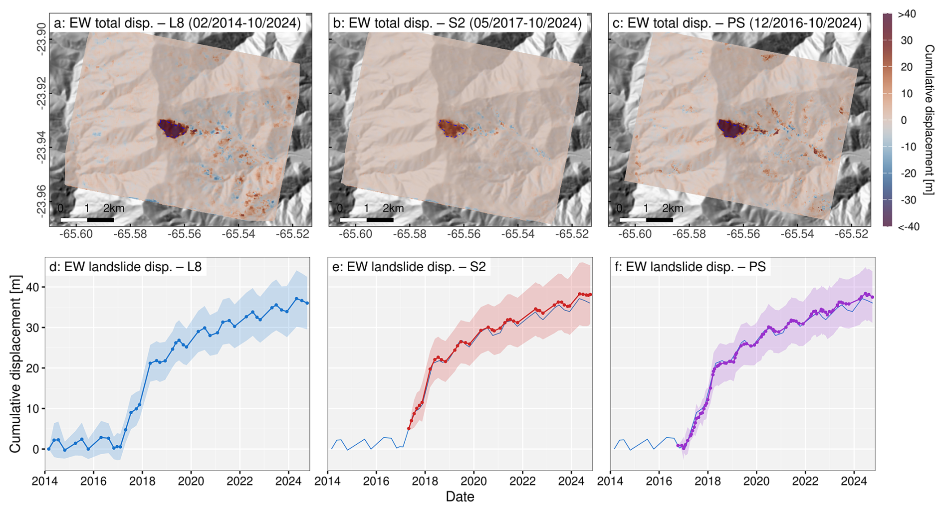
Figure 2 Map view of the total cumulative displacement estimated at each pixel after inversion for Landsat-8 (a), Sentinel-2 (b), and PlanetScope (c) networks over the respective time span covered by the available satellite data. The plots show the east-west (EW) component, which is most significantly affected. A figure for the north-south component can be found in the Supplement (Fig. S7). Panels (d) to (f) show the mean and standard deviation (ribbon) of the cumulative displacement estimated over the landslide surface (see dashed blue polygon in panels a–c) for all three data sets. For better comparison, the shorter time series of Sentinel-2 and PlanetScope were offset by the Landsat-8 displacement (blue line), approximated at their respective start date. A clear seasonal oscillation bias pattern is visible, requiring correction.

4.2 Impact of variable illumination

In addition to the described trends, all displacement time series (Fig. 2d–f) are characterized by seasonal oscillations with an average amplitude of approximately 1 m over the landslide surface (see Supplement, Fig. S8 for precise amplitudes). This pattern is not restricted to the Del Medio landslide, but occurs throughout the scene over stable terrain with variable magnitudes up to 5 m and more in areas largely affected by shadows (Fig. 3). Therefore, it can be assumed that the oscillation signal does not reflect the actual landslide motion. Instead, it is caused by changing illumination conditions throughout the year. An indication of this hypothesis is the strong relationship between the amplitude (and phase, see Figs. S9, S11, and S12) of the oscillation and the topography, as previously observed by Lacroix et al. (2019). The influence of other seasonal variables, such as the changes in humidity and vegetation cover, is disregarded due to the scarcity of vegetation at 4000 m, particularly in the upper part of the Del Medio catchment. We do not observe an east-west gradient of the signal strength that mimics moisture transport and vegetation-cover gradients in the catchment (the lower elevation eastern part of the catchment receives more moisture and has a higher vegetation cover). Dense deciduous vegetation may compromise correlation results of cross-seasonal correlation pairs in other study areas.

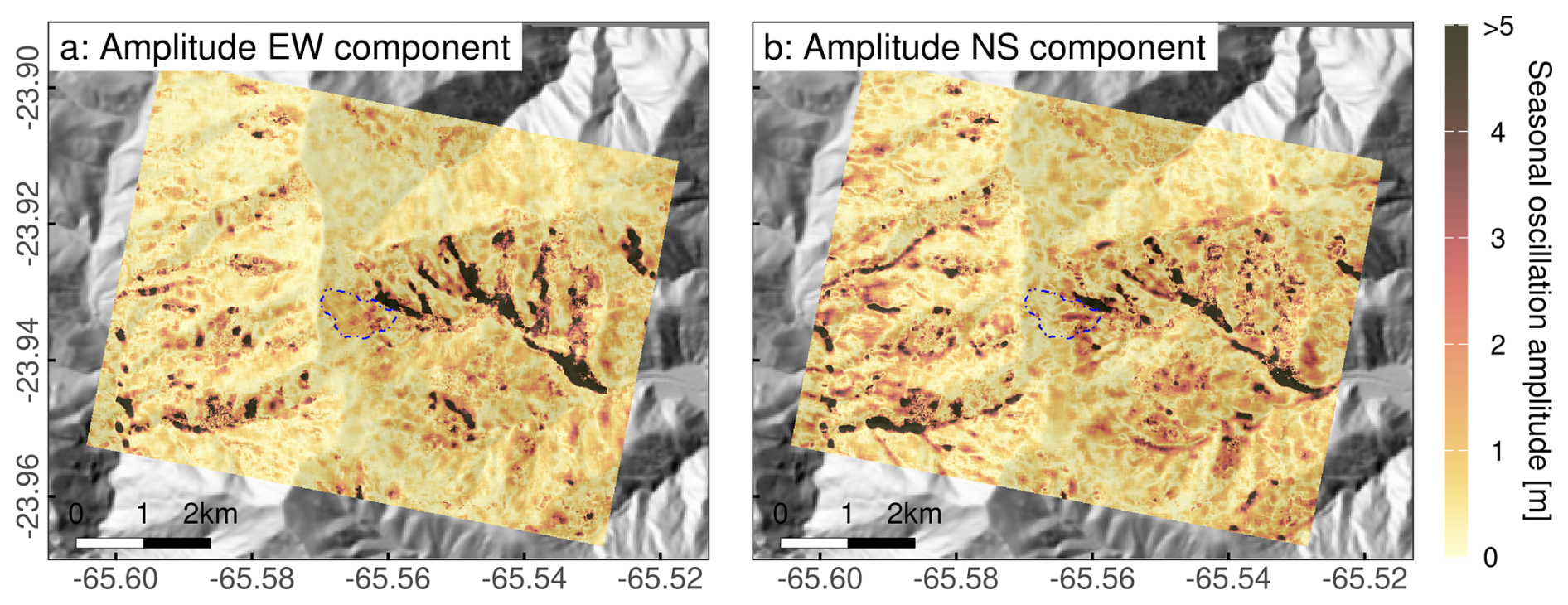
Figure 3 Amplitude of the seasonal oscillation in the PlanetScope inversion results for the east-west (EW) (a) and north-south (NS) (b) component. The amplitude was estimated by removing the long-term trend from the displacement signal and fitting a sine with a 1-year wavelength. The distribution of the phase component is illustrated in the Supplement (Fig. S9). Plots for Sentinel-2 and Landsat-8 can be found in the Supplement (Figs. S10 and S11). The dashed blue line outlines the landslide surface.

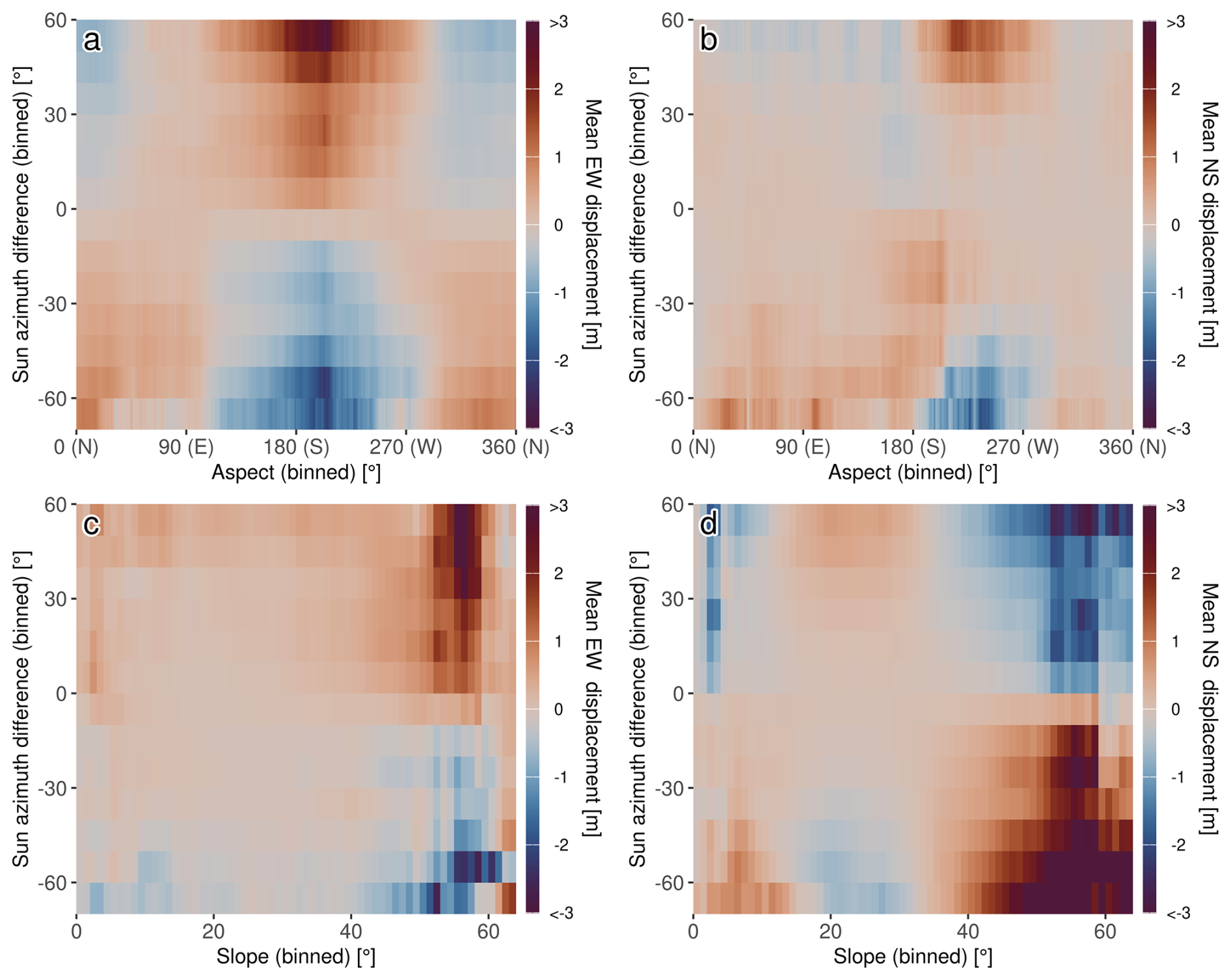
Figure 4 Mean displacement estimated over stable terrain in all 491 displacement maps retrieved from PlanetScope imagery. We binned pixels according to the sun azimuth difference between the correlated image pair (5° bins) and the terrain aspect (a, b) and slope (c, d), both in 1° bins. Sun azimuth differences were calculated by subtracting the solar position of the reference image from that of the secondary image. While over stable terrain the displacement is expected to be zero, we can observe a systematic error related to the terrain aspect at high sun azimuth differences. This relation also has a dependence on terrain slope. These measurement errors are the basis for the subsequent oscillation pattern when the network is inverted. Results for the sun elevation difference are similar and shown in Fig. S13 and the pixel counts per bin in Fig. S14.

Figure 4 shows the average displacement estimated over stable terrain in the PlanetScope displacement maps retrieved from image correlation. Through binning pixels by the aspect, slope, and the difference in sun elevation between the reference and secondary image, we note a distinct distribution of measurement errors. As measurement errors, we interpret any non-zero displacement assuming that the terrain surrounding the landslide has remained stable. The first observation is that the higher the difference in sun azimuth (and elevation, see Supplement, Fig. S13), the stronger the deviation from zero. Whether this discrepancy is positive or negative depends on the sign of the sun-angle difference. In addition, we note a particularly strong relation with terrain aspect: for the east-west component, there is a positive (eastern) and negative (western) measurement bias that peaks at slopes with a south-west facing aspect (180–270°). This is consistent with the direction of shadow extension, which is opposite to the sun's azimuth angle. For the PlanetScope scenes, the sunlight is coming from the north-east (60°) on average (Supplement, Fig. S2). For the north-south displacement component, we see a similar trend, but the relation is less pronounced. Regarding slope, steeper terrain generally corresponds to larger measurement errors, which is expected since shadowing effects are more pronounced in such areas.

The decadal displacement history of the Del Medio landslide, as described at the beginning of this section (∼ 35 m), clearly exceeds the seasonal bias in magnitude. Nevertheless, the presence of the seasonal oscillation pattern impedes our ability to assess smaller-scale magnitude variations that could point to velocity changes in response to a seasonal climate. We therefore evaluate mitigation strategies to reduce seasonal biases while preserving the true displacement signal as much as possible.

4.3 Impact of spatial resolution

One observation was a link between the seasonal bias magnitude and spatial resolution of the input images. We initially correlated imagery from all three satellite missions at their native resolution, only adjusting the correlation and subpixel refinement kernel size to be as comparable in meters as possible, taking into account the odd-integer constraint. However, we noticed that the lower-resolution Landsat-8 and Sentinel-2 correlation results were more strongly affected by seasonal biases than the 3 m PlanetScope displacement maps. A test with two scene pairs from PlanetScope and Sentinel-2 (similar dates) acquired under different illumination conditions (May and September 2020) resampled to 3, 6, and 9 m confirmed this observation (Fig. 5): Over stable terrain (estimated zero displacement), the seasonal bias increased significantly as the spatial resolution of the input imagery decreased. A similar observation was made by Antoine and Liu (2025), who found that correlation noise decreases when the images are upsampled. We attribute this effect to the subpixel refinement step of the correlation process, which refines the integer pixel match obtained from previous block matching. We use the mode that applies the Bayes expectation-maximization weighted affine adaptive window correlator, which is slow in runtime but recommended for high-quality results (Beyer et al., 2018). The effect of spatial resolution is also observed for other subpixel refinement methods and matching algorithms (Supplement, Figs. S15–S18). At lower image resolution, the pinpointing of the match within a larger pixel may be less precise. Furthermore, the variable number of pixels in the subpixel refinement window may have resulted in slightly different weights for different resolutions. To achieve a better comparability between satellite imagery from different sources and have a similar magnitude of seasonal biases, we therefore correlated all imagery only after resampling to a common 3 m resolution. An example of the combined effect of bias illumination variation and a moving target (artificially induced offset) at different spatial resolutions is shown in the Supplement (Figs. S19 and S20).

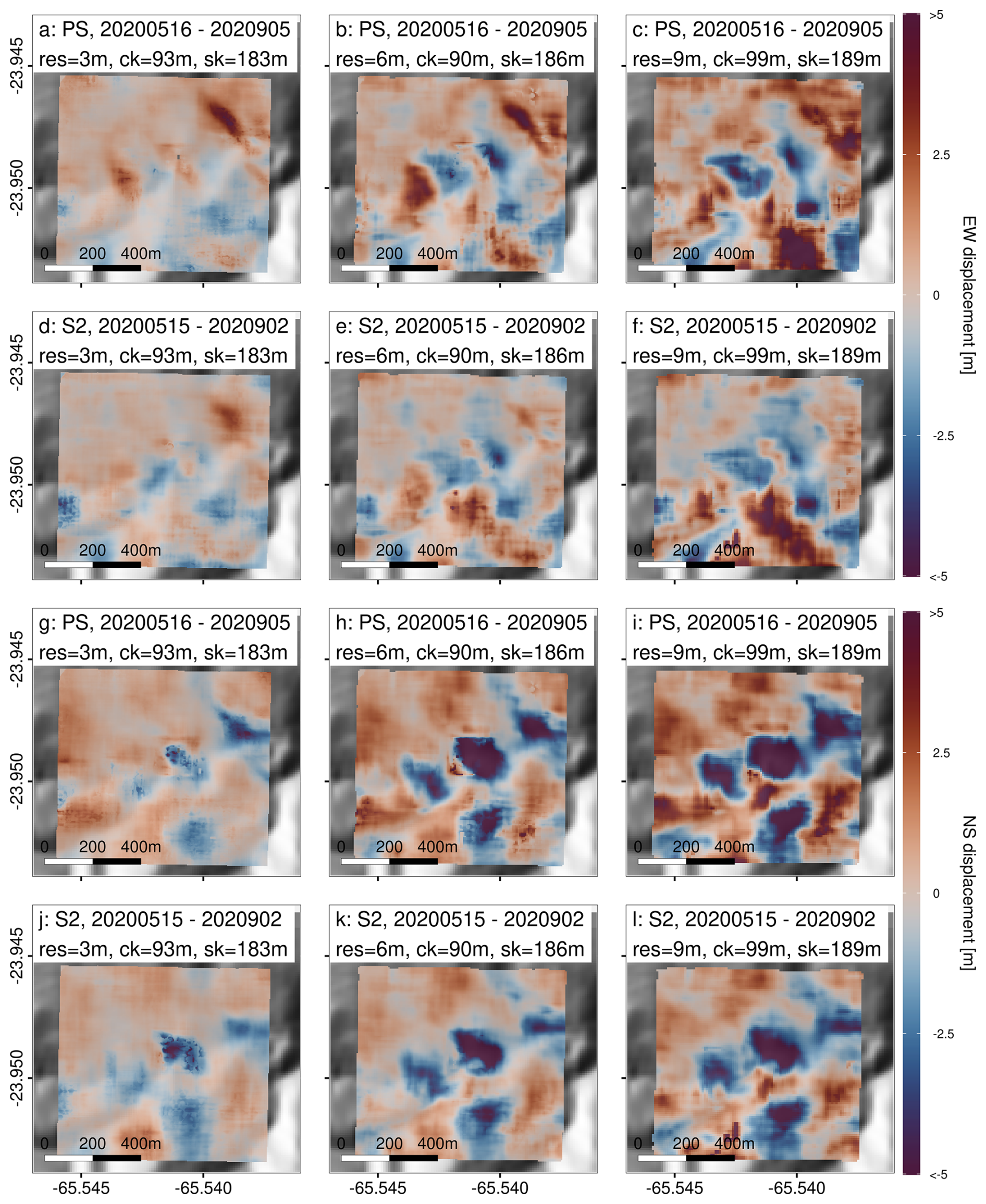
Figure 5 Displacement estimated from a cross-seasonal PlanetScope (16 May and 5 September 2020, first and third row) and Sentinel-2 (15 May and 2 September 2020, second and fourth row) image pair over a small sample area of stable terrain. Panels (a)–(f) show displacement in the east-west (EW) direction and panels (g)–(l) in the north-south (NS) direction. The plot illustrates the seasonal bias at different resolutions: satellite images were resampled to 3 m (first column), 6 m (second column), and 9 m spatial resolution (third column). Correlation and subpixel refinement kernel were kept approximately constant in terms of area (i.e., fewer pixels at lower spatial resolution). We find that as the resolution of the input imagery becomes coarser, the magnitude of seasonal measurement errors increases.

4.4 Comparison of seasonal bias mitigation strategies

The relationship between spatial resolution and measurement biases opens the door to mitigating seasonal oscillations by upsampling input imagery. However, while seasonal bias is reduced, it is not eliminated (see Fig. 3). In addition, longer processing times naturally limit the extent to which this strategy remains practical and call for alternative mitigation approaches. Therefore, we compare additional strategies to reduce seasonal bias in time-series inversion results, as described in Sect. 3.6.

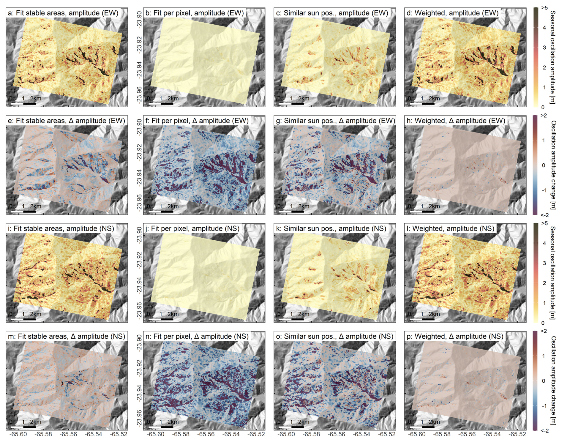
Figure 6 Amplitude of the seasonal oscillation pattern in the PlanetScope inversion results after the application of four different mitigation approaches. We plot the estimated amplitude of the seasonal oscillation bias after correction for the east-west (a–d) and north-south (i–l) component, as well as the change of amplitude in comparison with the uncorrected inverted timeseries (see Fig. 3) for the east-west (e–h) and north-south (m–p) component. The following approaches are compared: removal of the best-fit sine over stable terrain with common slope and aspect (first column); removal of the best-fit sine estimated per pixel (second column); inversion of a network with similarly illuminated image pairs only (third column); and weighting based on the difference in solar incidence angle (fourth column).

Figure 6 compares the effect of the four different mitigation strategies described in Sect. 3.6 on the seasonal oscillation amplitude. The first column shows the results after subtracting the best-fit sine over stable areas with common slope and aspect. This method reduces the estimated oscillation amplitude, particularly in areas heavily affected by shadows. For some pixels where the median fit per group exceeds the initial oscillation bias, the amplitude after correction increases. Over the landslide surface, amplitude changes are minor. The effectiveness of this correction method is based on the alignment between the reference DEM and the observed seasonal bias. Lacroix et al. (2019) used a 2 m stereo DEM, while we rely on the Copernicus DEM with 30 m spatial resolution that will not depict features whose shadows are well visible in the 3 m optical data. In addition, landslide topography changes over time, and the use of an outdated DEM may introduce unexpected artifacts (Mueting and Bookhagen, 2024). This limited resolution and temporal alignment, combined with the complex topography of our study area, could be the reason why the correction approach has limited success in reducing the oscillation bias over the Del Medio landslide.

The second column of Fig. 6 illustrates the result of subtracting the best-fit sine from the displacement time series of each pixel, irrespective of whether it covers moving or stable grounds. Naturally, this method is very effective at removing any seasonal oscillation from the displacement time series. It is independent of external topographic information and does not average signals over larger areas. However, over the landslide surface, a per-pixel fit does risk the partial removal of true seasonal responses. The strength of this potential alteration depends on the regularity of true seasonal response signal. The correction method is more successful at preserving irregular seasonal responses. For example, a displacement signal that does not accelerate during every rainy season can be reliably unmixed from seasonal bias, while a regular seasonal response would appear as a linear displacement signal after correction (Fig. S21). This mitigation strategy should therefore be applied with care, ideally when it can be ruled out that a moving body shows a regular seasonal response signal.

The third column of Fig. 6 depicts the effects of limiting correlation to scenes acquired under similar sun positions and the remaining seasonal bias estimated over the entire study area. This strategy proved to be effective in largely reducing seasonal oscillations and preserving the initial measurements, thereby avoiding the risk of altering true displacement signals through post-processing. The lower number of displacement fields in a network constrained by similar illumination conditions reduces the computational load, but it also allows errors related to other sources to propagate more easily. When connections are sparse, the relative importance of each measurement in a network is higher, increasing the impact of potential errors from other sources. In a densely connected network, on the other hand, the impact of a few erroneous displacements can be mitigated by redundancy of numerous pairwise measurements, leading to a reduction of uncertainties through time-series inversion (Charrier et al., 2022c). The lower number of connections is certainly a drawback of this mitigation approach. Suitable correlation partners may be sparse, particularly during the rainy period, and when other constraints (e.g., same view angle) are applied. As a result, the temporal resolution of the time series from similarly illuminated pairs is reduced. For example, for PlanetScope, only 60 time steps remain after applying sun elevation and azimuth angle thresholds, compared to 87 scenes for the full network. This makes it more difficult to precisely constrain the onset of changes in displacement rates. Having a larger number of suitable scenes to begin with (e.g., through near-daily PlanetScope acquisitions) can overcome this limitation.

The fourth column in Fig. 6 depicts the impact of introducing weights to the temporal inversion. Compared with the other mitigation approaches, weighting showed the least improvement in reducing the amplitude of seasonal biases. Changes are mostly constrained to the heavily shadowed areas, where positive and negative amplitude changes are observed. Further experiments with a higher resolution DEM (the 30 m topographic information may not be sufficient to resolve effects that are observed in the higher-resolution optical data), combined weighting factors, or improved weight scaling could yield better results.

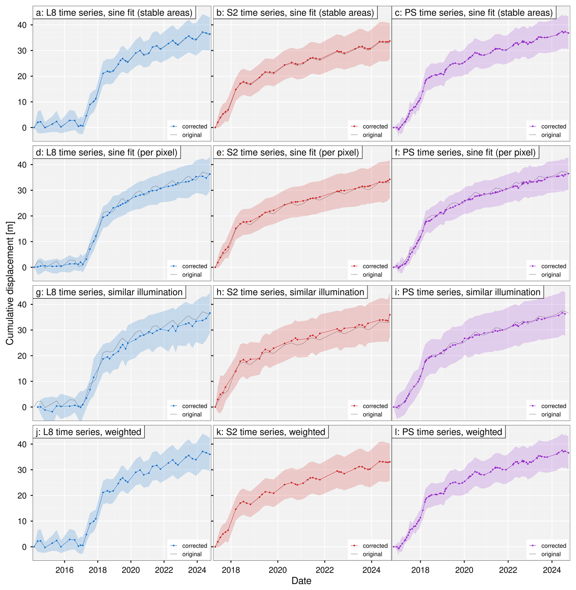
Figure 7 Average displacement time series over the Del Medio landslide after mitigation of the seasonal bias component for Landsat-8 (first column), Sentinel-2 (second column), and PlanetScope (third column). The effects of four mitigation approaches are plotted: removal of the best-fit sine estimated over stable terrain grouped by common slope and aspect (first row), removal of the best-fit sine per pixel (second row), considering similarly illuminated image pairs only (third row), and weighting based on solar incidence angle (fourth row). For comparison, the uncorrected time series are plotted in gray. Ribbons indicate the standard deviation.

The time series extracted over the Del Medio landslide for all satellites after applying the four different correction approaches are plotted in Fig. 7. Subtracting the best-fit sine per pixel and the selection of similar illuminated image pairs for the inversion reduced seasonal oscillations most reliably both over the landslide and surrounding terrain. Some problematic regions remain along steep and heavily shadowed slopes throughout the Del Medio catchment, where the correlation often fails or produces mismatches. Here, the residuals for the estimated sine function are high. If supported by the correlator, shadows could be masked prior to the image matching to reduce their impact (Provost et al., 2022).

Although subtracting the best-fit sine per pixel provides the smoothest time series over the surface of the landslide (Fig. 7) and the highest overall reduction of seasonal displacement bias (Fig. 6), it can also alter true seasonal responses in the movement of the landslide, especially when these occur every rainy season (Fig. S21). The observed displacement time series over the Del Medio landslide suggests that changes in velocity have occurred, but not of regular magnitude and timing (occurring every year). Considering this, we would argue that the sine fit per pixel could be applied to correct seasonal biases at the Del Medio landslide without greatly modifying the true displacement signal, at least not beyond the uncertainties introduced by measurement errors linked to other factors. However, since there are no ground control data available to fully confirm the absence of a regular seasonal response in landslide motion, we base subsequent interpretations of the landslide kinematics on the time series obtained from similarly illuminated pairs only. These results exhibit slightly higher variability and lower temporal resolution, especially for Sentinel-2 and Landsat-8 data, which is a result of the lower number of eligible correlation pairs.

To compensate for the lack of ground control data, we performed an additional evaluation of the impact and reconstruction accuracy of all mitigation approaches using a synthetic example (Figs. S22–S24). Over stable ground, we moved a rectangular patch according to a known displacement signal in the available PlanetScope imagery (PSB.SD only). The simulated signal consists of a linear displacement trend (10 m total displacement) with a single acceleration event occurring during one of the rainy seasons. We performed this analysis (i) over a well-illuminated slope with a similar orientation as the landslide and (ii) over complex terrain heavily affected by shadows (see Fig. S22). We observe that in the well-illuminated example, the acceleration introduced to the time series is captured very well, and as the seasonal oscillation bias is low, little to no correction is required (Fig. S23). In the topographically more complex area suffering from shadow effects, the reconstruction is much more difficult. Here, the sine-per-pixel correction achieves the best results, but only for responses irregular in timing, which can be well separated from seasonal bias (Fig. S24). These additional tests demonstrate that even in close proximity, the effectiveness of different mitigation strategies in accurately reconstructing observed displacement can vary. In general, the presence of shadows in complex terrain leads to greater uncertainties in the reconstructed displacement, even after mitigation of seasonal biases. The need for and choice of a suitable correction method should always consider the monitored area, expected behavior of the monitored target, and the number of available acquisitions.

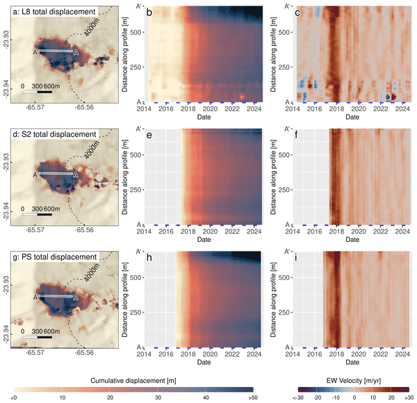
4.5 Spatially variable landslide motion

The higher standard deviations of cumulative displacement measured over the Del Medio landslide following the relative uniform acceleration in the beginning of 2017 (see Fig. 7) suggest that different parts of the landslide have moved at different speeds following this event. Therefore, in addition to the averaged landslide motion, we investigate the cumulative displacement along a horizontal profile across the landslide using the displacement estimates obtained from similarly illuminated image pairs. Figure 8a, d, and g show a close-up of the total displacement accumulated during the observation period, as well as the location of the selected profile line. Here, we find that the highest displacement magnitudes are concentrated along the upper scarp and a central block at about 4000 m elevation. Taking into account the temporal evolution of the cumulative displacement along a horizontal profile across the landslide (Fig. 8b, e, h), we observe that these parts moved faster after the 2017/2018 monsoon season. Subsequent continuous displacement was interrupted by an acceleration at the upper scarp at the end of 2021 (near point A^′). These observations are consistent across all three satellite data sources, but are clearest in the densely sampled PlanetScope time series. To better highlight the points of acceleration, we have calculated the east-west velocity from the smoothed displacement time series (Fig. 8c, f, i). Velocities may become negative when the estimated movement has a westward (uphill) direction, which is the result of measurement errors affecting the lower, heavily shadowed part of the profile (∼ 0–150 m along profile), particularly affecting the Landsat-8 displacement timeseries. The reactivation of the landslide in early 2017, as well as the acceleration during the monsoon season of 2017/2018, are clearly visible. In addition, the PlanetScope time series hints at two additional phases of elevated velocities in late 2018 and early 2020. The pure downhill (positive, eastward) motion suggests the reliability of these measurements. However, the displacement magnitude is relatively low and is largely obscured by noise in the Landsat-8 and Sentinel-2 displacement time series. These two small accelerations are not well detectable when mitigating seasonal biases through a per-pixel sine fit (Supplement, Fig. S25); however, they may have been smoothed by the correction method. The acceleration that occurred during the monsoon season of 2021/2022 in the upper part of the landslide is more visible, especially in the PlanetScope time series. After that, the landslide appears to have moved uniformly until the end of the observation period.

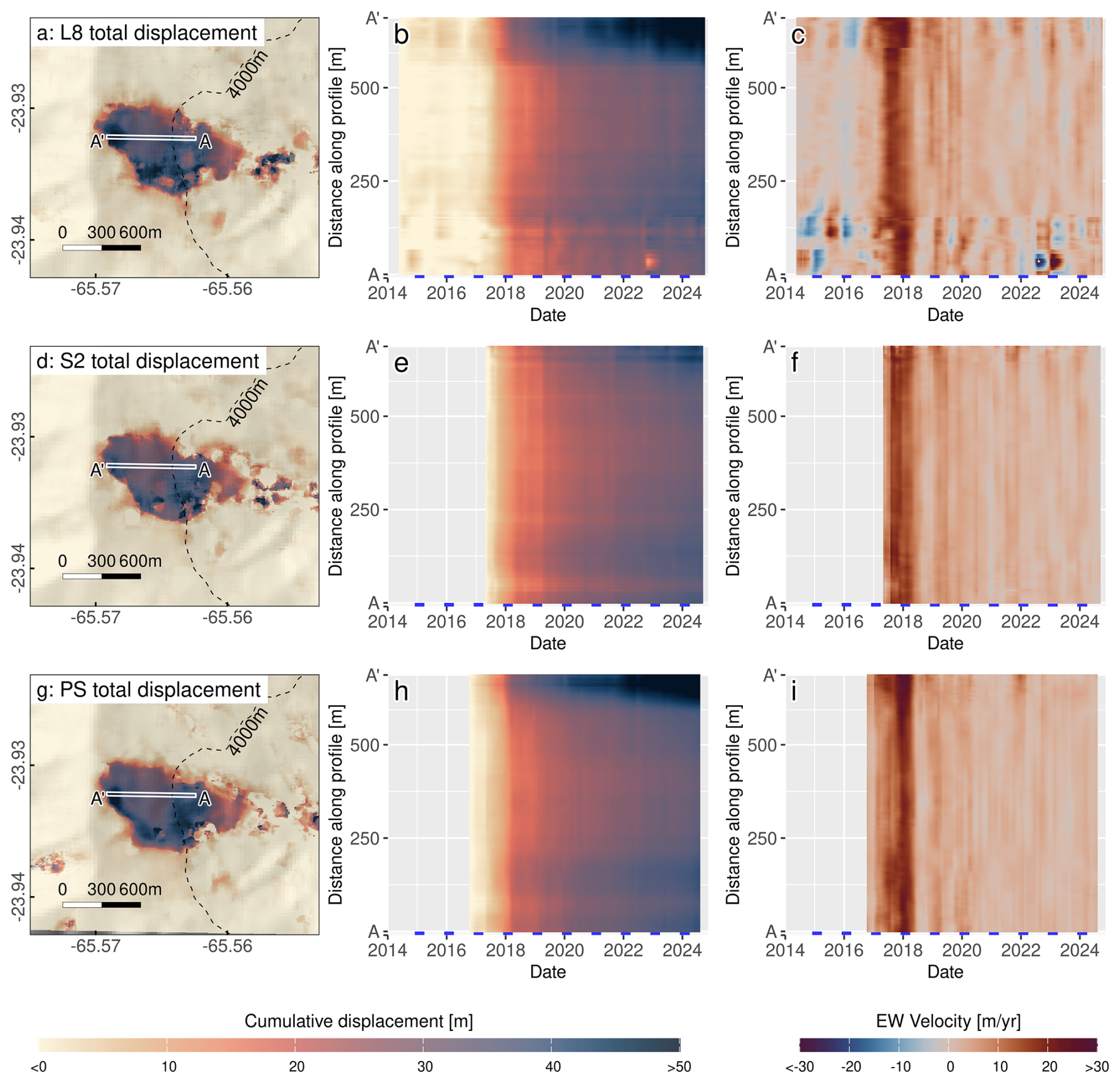
Figure 8 Spatially variable displacement rates along a profile over the Del Medio landslide. The maps in the first column show the total displacement estimated over the landslide throughout the observation period, the location of the profile, and the 4000 m contour line for Landsat-8 (a), Sentinel-2 (d), and PlanetScope (g). The cumulative displacement through time along this profile is plotted in the second column for the respective satellites. To better identify periods of acceleration, we derived the velocity from the smoothed (rolling mean with a half-year window) cumulative displacement, as shown in panels (c), (f), and (i). For both the second and third columns, we indicate the monsoon season (December–March) with blue bars along the x-axis. Seasonal biases were compensated for by considering only image pairs with a similar illumination. Results for the correction based on subtracting the best-fit sine estimated per pixel can be found in the Supplement (Fig. S25).

5 Discussion

5.1 Drivers and preconditioning factors of landslide activity

The mitigation of seasonal biases allowed us to clearly identify three, potentially five, acceleration phases in the displacement history of the Del Medio landslide that all fall into the rainy seasons: the initial reactivation during the rainy season of 2016/2017, a steep acceleration at the beginning of 2018, two potential low-magnitude responses in late 2018 and early 2020, and a smaller acceleration in the monsoon season of 2021/2022 that was constrained along the upper scarp of the landslide. In the following section, we evaluate potential triggers and preconditioning factors for these three acceleration phases.

In the Andes of Argentina, rainstorm events and seismic shaking in conjunction with geological preconditioning in the form of structures and weathered lithology were identified as the primary triggers of landslides (Moreiras and Coronato, 2009). After assessing all seismic events recorded in the USGS earthquake catalog (U.S. Geological Survey, 2025) in a 100 km radius of the study area, as well as the catalog of the Instituto Nacional de Prevención Sísmica (https://www.inpres.gob.ar/, last access: 9 August 2026), we concluded that while there were a few earthquakes in the Humahuaca basin, these were either of very low magnitude, large depth, or not temporally coincident with the observed acceleration phases. This leaves precipitation as a likely candidate for triggering reactivation in the rainy season of 2016/2017, as well as subsequent accelerations. Several studies have linked landslide reactivation or acceleration to prolonged and intense rainfall (e.g., Uhlemann et al., 2017; Handwerger et al., 2019a; Xue et al., 2022; Sreejith et al., 2024). At the Del Medio landslide, the observed accelerations can fall close to or into the summer monsoon season (approximately from December to March), supporting the hypothesis of precipitation as the primary forcing. Due to a lack of ground measurements, we approximate precipitation affecting the Del Medio landslide using data from the Global Precipitation Measurement Mission (GPM) (∼ 10 × 10 km grid size) (Huffman et al., 2023). The daily sum of precipitation together with the cumulative displacement time series at the upper scarp of the Del Medio landslide, including all potential acceleration phases, is shown in Fig. 9a–b. In addition to precipitation, we also consult ERA5 land surface temperatures (Hersbach et al., 2020) (Fig. 9c) because the landslide is located at elevations above 4000 m, where freeze-thaw processes play a role. Similar permafrost-related patterns were described in the geographic vicinity in the Valles Calchaquíes (e.g. Blöthe et al., 2025; Falaschi et al., 2014). Since we do not find evidence that the landslide has accelerated during the monsoon season every year, and also showed responses of largely different magnitudes, we focus on meteorological extremes. Different studies have shown that landslide motion can be significantly influenced by extended droughts and periods with exceptional rainfall (e.g. Handwerger et al., 2019a; Hopquin et al., 2025), and particularly the shift between wet and dry extremes can lead to catastrophic failures (Handwerger et al., 2019b).

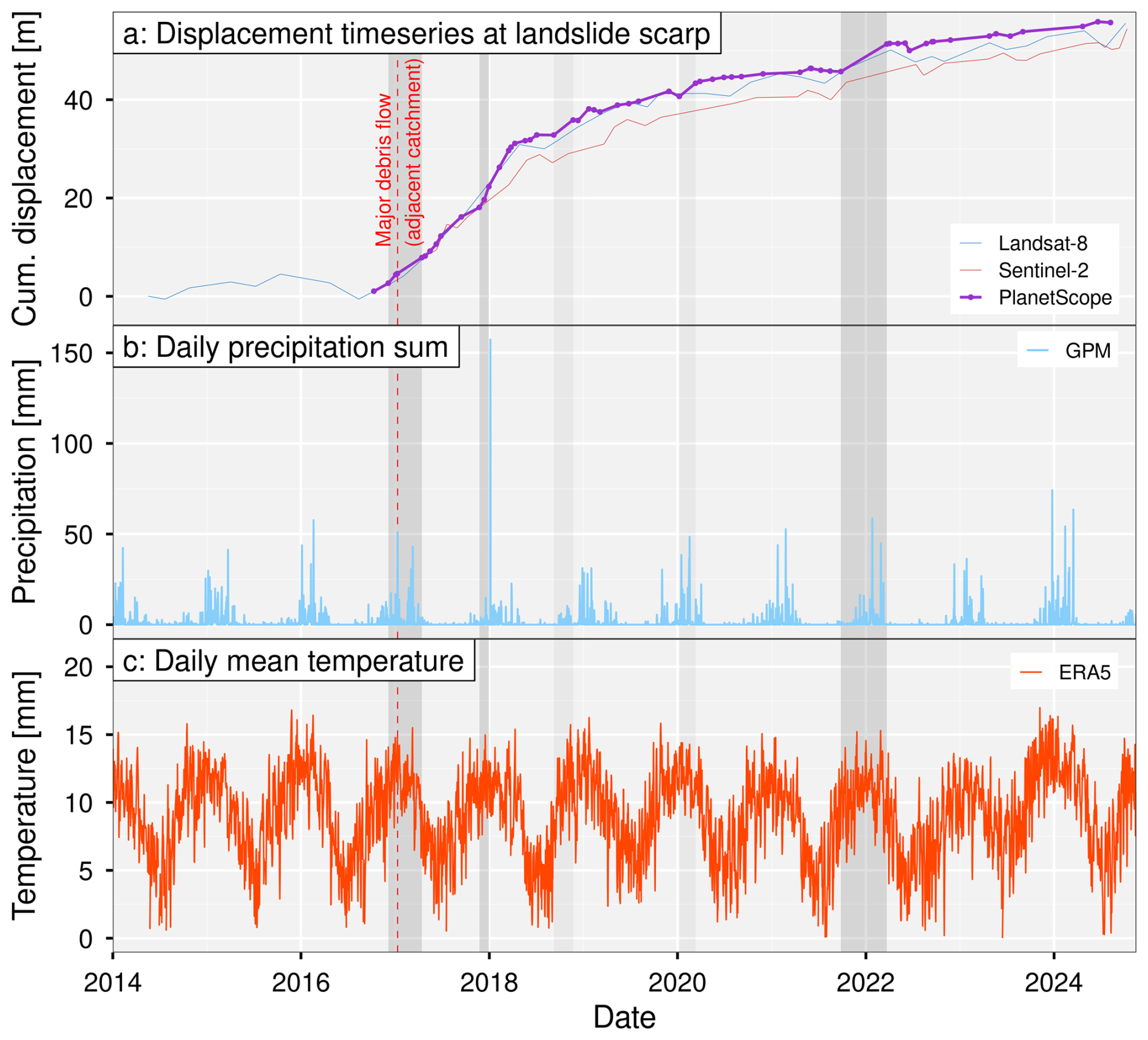
Figure 9 (a) Cumulative displacement time series at the scarp of the Del Medio landslide (upper 30 m of the profile shown in Fig. 8) estimated from PlanetScope data in comparison with Sentinel-2 and Landsat-8. Seasonal biases were mitigated by selecting image pairs with similar illumination only. The debris flow event that occurred in the neighboring Los Filtros basin on 10 January 2017 (Angillieri et al., 2020), following heavy rainfall, is marked by a dashed red line. Clear increases in displacement between consecutive acquisitions are highlighted in gray. Two potential accelerations falling in late 2018 and early 2020 are marked in light gray. Panel (b) shows the daily precipitation estimated by GPM (Huffman et al., 2023). ERA5-derived mean daily land surface temperatures (Hersbach et al., 2020) are plotted in panel (c).

In the Del Medio catchment, the assessment of precipitation and temperature over the entire 10-year study period reveals that none of the years linked to a landslide acceleration phase have been particularly wet or warm. Still, the large differences between dry and rainy periods are evident, and although there is no sign of prolonged episodes of extreme rainfall or drought, the precipitation time series does record individual days with heavy rainfall exceeding 50 mm. These events are not evident in the lower resolution ERA5 climate reanalysis dataset (∼ 31 × 31 km grid size), likely due to variable precipitation rates with localized convective events on orographic barriers, leading to high rainfall amounts (e.g. Bookhagen and Strecker, 2008). Two instances of very high rainfall recorded within 24 hours occurred close to the two acceleration phases with the largest magnitude: the initial reactivation of the landslide during the rainy season of 2016/2017 and the acceleration in the following year. The heavy rainfall event in January 2017 is also described in the literature, because it triggered a major debris flow in the neighboring Los Filtros basin to the north on January 10, 2017, which was considered the most catastrophic event in the last 40 years (Angillieri et al., 2020). The debris flow occurred as a result of heavy rainfall reported as ∼ 170 mm between 08:00 and 10:00 am local time in the area (Angillieri et al., 2020) (much higher than the rates suggested by the GPM time series). In pre- and post-event images, Angillieri et al. (2020) found signs of reactivation of a previously inactive landslide, as well as several small slope failures in the Los Filtros basin, which supplied loose material to the debris flow. For the Del Medio catchment, only small changes in the catchment and a minor flow in the south of the basin were observed. For the subsequent rainy season, we found no reports, but the GPM timeseries records a maximum rainfall of 157 mm on 5 January 2018 (Fig. 9b). In the Del Medio catchment, precipitation affects slopes that are already weakened due to their geological preconditioning. Inherited fault structures that bound the basin (Fig. 1) and an exposed lithology of heavily fractured phyllites create preferential flow paths that allow fast infiltration. In addition, freeze-thaw cycles that act at high elevations further degrade rock strength. In such an environment, a single heavy rainstorm may suffice to alter stability conditions beyond a critical threshold to set a slope in motion. Therefore, we suggest that the heavy rainfall on 10 January 2017, could have been the final trigger to set a landslide in motion, which was already in a fragile state.

Also, the other acceleration phases of 2018/2019, 2019/2020, and 2021/2022 coincide with higher precipitation rates. More satellite acquisitions during the rainy season would be needed to better link the onset of these accelerations to individual rainfall events.

Besides the link to precipitation, we observed that the moving surface of the landslide identified in this study does not fully align with the scarp of the 2009 rockfall event, but extends further uphill (Fig. 1). The large mass removal in 2009, which concentrated towards the center and toe of the currently active landslide (Fig. S1b), potentially reduced support for the upslope areas. This destabilization may explain the elevated displacement rates observed in the upper part of the landslide.

5.2 Comparison between the different satellite missions

We have used data from three different satellite missions to analyze the landslide displacement history and also to cross-compare the derived measurements. For better comparability between all missions, we not only resampled data to a common resolution but also reran the inversion exclusively using correlation pairs falling into a common time span between March 2020 and October 2024. In this way, we compare Landsat-8 and Sentinel-2 data to only the newest generation of PlanetScope (PSB.SD instrument), and also cover a time span with moderate displacement rates where a few days of difference between start and end date have a lower impact. From the inversion results, we have calculated the difference in the total estimated displacement before and after seasonal bias correction through a sine fit, as well as the average displacement across the landslide surface (Fig. 10). The strategy of selecting image pairs with similar illumination conditions was omitted as it largely reduced the number of connections remaining in the networks. From the previous observations, we conclude that the period between 2020 and 2024 showed largely uniform displacement (except at the landslide scarp), so applying the per-pixel sine fit should not severely bias the time series. We find that on the surface of the landslide, the estimated average and standard deviation of displacement are largely consistent between all satellite missions, despite the difference in spatial resolution of the native images. In particular, Sentinel-2 measurements align well with the PlanetScope-derived displacements, while Landsat-8 shows a slightly lower estimate. Throughout the study area, the displacement difference between all satellites is centered around zero. The standard deviations are highest between Landsat-8 and PlanetScope with ±2.97 m before correction and slightly lower for Sentinel-2 and PlanetScope with ±2.5 m. Both values improve to ±2 m after reducing seasonal biases. Nevertheless, the highest differences remain concentrated along high-relief areas affected by shadows. The closest correspondence is achieved between Sentinel-2 and Landsat-8 with a standard deviation in the total estimated displacement of ±1.89 m before and ±1.58 m after seasonal correction.

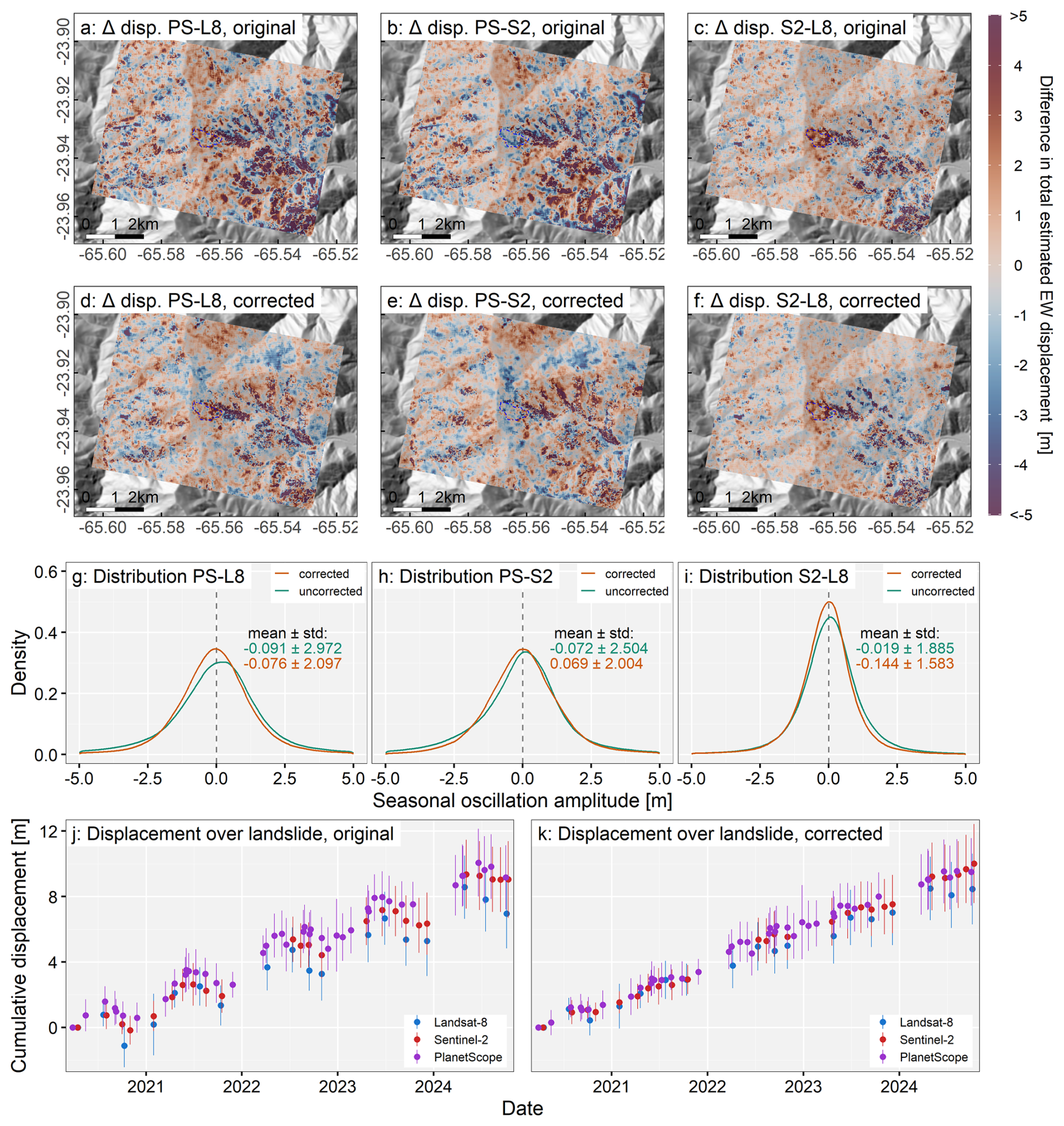
Figure 10 For a common time span between March 2020 and October 2024 over the Del Medio landslide, we have estimated the difference between displacement derived from Landsat-8, Sentinel-2, and PlanetScope (PSB.SD instrument only). Panels (a)–(c) show the difference in the total estimated east-west displacement after inversion, panels (d)–(f) show the difference with the seasonal oscillation bias corrected through a best-fit sine per pixel. The distribution of differences throughout the study area for both original (uncorrected) and corrected raster differences is depicted in panels (g)–(i). Finally, the mean and standard deviation of displacement over the landslide surface (outlined by a dashed blue polygon in panels a–f) are plotted in panels (j) and (k) based on the original (j) and sine-corrected (k) time series.

With no ground control data available for the Del Medio landslide, the large correspondence between three independent data sources gives confidence in the validity of the observed trends and measurements. The strong alignment between the measurements may partially relate to the upsampling strategy to a common 3 m resolution. In addition to the reduction of seasonal biases (Sect. 4.3), correlation noise was shown to increase linearly with decreasing resolution of input imagery that can be achieved by upsampling (Antoine and Liu, 2025). Our results indicate that at a common grid resolution, Sentinel-2 and Landsat-8 can be used to derive displacements with similar precision as PlanetScope data, despite their lower native sampling distance. Their extensive archives make both missions a valuable resource for assessing long-term displacement histories, and scenes are commonly less affected by complex co-registration errors compared to PlanetScope (Mueting and Bookhagen, 2024). However, only acquisitions with an initially higher resolution will allow capturing small landslides (Lacroix et al., 2018), small-scale variations, or the precise outline of moving objects. Even more important is the high revisit time, which increases the chances of cloud-free acquisitions during the rainy season. This is a prerequisite for studying slope movements in seasonal climates using optical data, but also increases the number of available scenes when applying pairing methods, e.g., based on similar illumination.

6 Conclusions

We successfully derived a decade-long displacement time series based on the temporal closure of pairwise displacement measurements using Landsat-8, Sentinel-2, and PlanetScope data for the large and slow-moving landslide in the Río Del Medio catchment. Its location in the transition zone between the Altiplano-Puna plateau and the Andean foreland exposes the landslide to a highly seasonal climate with intense rainfall during the summer monsoon season. The geological evolution of the study area has generated shear zones and highly fractured rocks that act as preferential pathways for water infiltration, leading to reductions in shear strength and increased susceptibility to landslide triggering and accelerations. Our analysis focused on the mitigation of seasonal measurement biases to identify potential feedback mechanisms between rainfall and landslide movement. A key challenge in using optical imagery for displacement measurements, particularly in high-relief areas, is the seasonal bias introduced by variable illumination and shadows, which results in artificial seasonal oscillation patterns. This bias was observed to be systematic and strongly related to topography and illumination differences. We evaluated different mitigation strategies.

First, we observed that lower-resolution Landsat-8 and Sentinel-2 correlation results were more strongly affected by seasonal biases than the 3 m PlanetScope correlations. By resampling Landsat-8 and Sentinel-2 imagery to the 3 m resolution of PlanetScope, a first reduction in seasonal bias was achieved, enhancing comparability across platforms, but increasing processing time and data volume.

Second, we modeled and removed seasonal oscillations by fitting a sine wave with a fixed frequency of one year to the detrended signal. This approach can be applied to stable areas with common slope and aspect, which creates a dependency on an external reference DEM, or per pixel, which may partially remove true seasonality in the displacement time series. Both approaches are straightforward to implement, but require multi-annual data to provide a robust fit. For the Del Medio landslide, the per-pixel approach proved to be most effective at removing periodic oscillations, but may also remove regular seasonal responses in landslide motion.

Third, we restricted correlation pairs to similar illumination conditions. The seasonal bias was also successfully reduced by defining maximum sun azimuth and elevation difference thresholds. However, the effectiveness of this method depends on the selection of a suitable threshold for the illumination difference. Thresholding also largely reduces the number of correlation pairs, making it applicable only in cases when abundant satellite data is available. Here, the high temporal resolution of the PlanetScope data is an advantage. In addition, sparse networks may allow other errors to propagate more easily into the derived displacement time series.

Lastly, we experimented with spatially variable weights, taking into account local topography and sun-position difference between the correlated image pairs. This method, however, was least effective, indicating that other weighting factors, e.g., based on temporal changes, may be more suitable.

For subsequent analyses, we considered the time series derived from similarly illuminated pairs, which is recommended in the absence of ground control data as it avoids any subsequent alteration of the obtained measurements and thus potential removal of true seasonal landslide motion.

The mitigation of seasonal biases decreased systematic errors, which helped to clearly identify changes in the kinematic behavior of the Del Medio landslide, specifically noting three distinct accelerations: the initial reactivation in early 2017, a steep acceleration in the rainy season of 2017/2018, and a smaller acceleration phase in late 2021/early 2022. Two smaller and less pronounced increases in landslide velocity were observed in late 2018 and early 2020. The reactivation of the landslide occurred during the 2016/2017 rainy season after a relative quiescence period of at least three years. The landslide accumulated approximately 20 m of displacement between January 2017 and March/April 2018. Subsequently, average displacement rates decreased to about 2.5 m yr⁻¹ until the end of the observation period in October 2024. Displacement rates varied spatially, with higher values concentrated along the landslide scarp.

While our findings do not support a systematic annual feedback between seasonal climate and landslide motion each year, the observed acceleration phases strongly suggest that precipitation is a primary forcing factor. The onset of all observed accelerations coincided with increased precipitation and could be linked to individual heavy rainstorms recorded in the precipitation time series, such as the one in January 2017 that also triggered a major debris flow in the neighboring watershed. The susceptibility of the slopes of the Del Medio catchment to sliding is attributed to preconditioning factors, including inherited fault structures, weakened lithologies (phyllites), and freeze-thaw processes occurring at high altitudes (up to 4500 m above sea level).

Our observations highlight the challenges of interpreting displacement time series derived from optical satellite data when both velocities and measurement bias are correlated with seasonality. By evaluating different mitigation strategies, we outline strategies towards improved management of seasonal measurement bias. This can help to reduce systematic errors in the displacement time series and contribute to a better understanding of the true feedback mechanisms between seasonal precipitation and slope movements.