Influence of groundwater seasonality on suspended sediment dynamics, in a 20 km² Mediterranean mountainous catchment

This study investigates the interplay between groundwater and surface runoff in controlling suspended sediment dynamics within the Galabre catchment, a 20 km² Mediterranean mountainous catchment characterized by extensive badland areas. Using an End-Member Mixing Analysis framework that accounts for event-specific variability in end-member chemistry, the study quantifies surface runoff and groundwater flows during 26 rainfall–runoff events from three hydrological years.

Hydrological analyses reveal that groundwater flow is the major contributor to streamflow, accounting for approximately 75 % of the event flow on average. Groundwater response varies substantially between seasons, with mean peak flows increasing from 2.5 ± 2.1 m³ s⁻¹ in spring/summer (May–September) to 5.9 ± 5.4 m³ s⁻¹ in autumn/winter. While both surface runoff and groundwater flows increase with event rainfall accumulation, groundwater flow shows a stronger dependence on rainfall accumulated over the preceding 15 d, emphasizing the influence of antecedent catchment wetness and long-term hydrological connectivity.

Hydrosedimentary analyses further demonstrate that suspended sediment concentrations (SSC) correlate more strongly with surface runoff flow rate than with flow rate (Q), emphasizing the dominant role of surface runoff in sediment detachment and transport on hillslopes. Marked seasonal differences in hydrosedimentary processes were observed. Spring/summer events, driven by short and intense rainfall, produce low-flow responses with high suspended sediment concentration and exhibit anticlockwise SSC–Q hysteresis loops. This suggests that these fine sediments could be mobilized from sources located relatively far from the outlet. The high suspended sediment concentrations and moderate flow rate in the river network likely lead to sediment deposition in the river network. Conversely, autumn/winter events, driven by prolonged low-intensity rainfall, and characterized by enhanced groundwater flow, produce high flow responses, with low suspended sediment concentration, and clockwise SSC–Q hysteresis loops. This hysteresis shape indicates close sediment sources that are likely associated with riverbed sediment remobilization. These findings reveal a fundamental seasonal shift from primary (i.e. hillslope mobilization) to secondary (i.e. riverbed remobilization) erosion processes, controlled by the seasonal variations of groundwater flow throughout the year.

1 Introduction

Improving the understanding of catchment-scale erosion rates and suspended sediment (SS) dynamics remains a major contemporary challenge in environmental science. SS fluxes, comprising both organic and inorganic particles transported in suspension, represent approximately 70 % of the total annual sediment load conveyed by rivers to the oceans (Vercruysse et al., 2017). These fluxes play a crucial role in landscape evolution, ecosystem functioning, and the redistribution of nutrients within fluvial systems (Owens, 2020). However, SS transport is also associated with numerous environmental and economic concerns. From an environmental perspective, SS dynamics strongly influence water quality, as fine particles can adsorb and convey both contaminants and nutrients (Francke et al., 2014; Brown, 1981; Pimentel, 2006; Glaser et al., 2023). Economically, sediment transport can hinder river navigation, compromise the stability of riparian infrastructure, and reduce the storage capacity of reservoirs as well as the recreational value of aquatic environments (Francke et al., 2014; Syvitski et al., 2005). These challenges are particularly pronounced in mountainous regions, where SS yields are typically high and exert a major control on sediment delivery to downstream lowland river systems (Navratil et al., 2010; Mano et al., 2009). In particular, Mediterranean mountain environments are characterized by intense storm events and the widespread presence of highly erodible and steep badland areas (sparsely vegetated terrains with exposed bedrock) resulting in substantial sediment delivery from hillslopes to riverbed during rainfall runoff events (Lloyd et al., 2016; Mano et al., 2009; Dedkov and Moszherin, 1992; Tropeano, 1991; Lenzi and Marchi, 2000; Nadal-Romero et al., 2008a; Mathys et al., 2005; Cantón et al., 2001; Romero-Díaz et al., 1999). In this context, identifying and prioritizing the processes that control erosion and SS transfer is of critical importance. Nevertheless, despite decades of research, the spatial and temporal variability of SS production, transport, and deposition in mountainous catchments remains poorly understood, mainly due to the lack of long-term field observations (Vercruysse et al., 2017; Owens et al., 2005; Navratil et al., 2010; Lawler, 2005; Nadal-Romero et al., 2008a).

SS inputs in the river originate from multiple sources, generally categorized as primary and secondary. Primary erosion refers to the initial detachment of soil particles from hillslopes, driven primarily by raindrop impact, surface runoff (SR) entrainment, and mass movement processes (Tolorza et al., 2014; Ellison, 1944; Gilley and Finker, 1985; Bryan, 2000). In Mediterranean mountainous regions, a substantial source of primary erosion comes from badland areas, where weathering processes such as biological activity and frost-cracking generate substantial stores of readily mobilizable sediment (Ariagno et al., 2022; Collins and Walling, 2004; Romero-Díaz et al., 1999; Nadal-Romero et al., 2008a). Once detached, particles may be transported downslope by SR into stream channels and subsequently exported from the catchment by river flow. Alternatively, they may undergo temporary deposition on hillslopes or within the riverbed, from which they can later be remobilized during subsequent rainfall–runoff events (Navratil et al., 2010; López-Tarazón et al., 2011; Park and Hunt, 2017; López-Tarazón et al., 2010). The magnitude of SS export is primarily controlled by rainfall intensity and river flow rate (Q), but numerous interacting factors modulate this relationship. These include sediment availability on slopes (Bača, 2008; López-Tarazón et al., 2010), spatial variability in topography, lithology, and soil erodibility (Uber et al., 2021; Mathys et al., 2005; Carriere et al., 2020; Navratil et al., 2011; Evrard et al., 2011), catchment scale (Goodrich et al., 1997; Ke and Zhang, 2024; Mayor et al., 2011), transport capacity of surface runoff (Vercruysse et al., 2017), seasonal variations in weathering processes (Ariagno et al., 2022; Gallart et al., 2002), heterogeneity in vegetation cover (Romero-Díaz et al., 1999; Chaves et al., 2008; Zuazo and Pleguezuelo, 2009; Mohr et al., 2013; Cotel et al., 2020; Vanacker et al., 2007; Shakesby, 2011; Navratil et al., 2011; Duvert et al., 2010), or spatial and temporal variability in rainfall intensity (Uber, 2020; Navratil et al., 2012, 2011; Tuset et al., 2016; Klein, 1984).

In addition to hillslope-derived sediments, secondary erosion processes contribute substantially to SS export through the remobilization of previously deposited material within the river network during earlier rainfall–runoff events. The remobilization of stored sediments is governed by particle characteristics and hydraulic conditions, including flow rate, shear stress, and stream power (Park and Hunt, 2017), leading to pronounced both short- and long-term temporal and spatial variability in riverbed sediment storage. Long-term variations in sediment storage and river morphology can be influenced by factors such as land-use change, channel vegetation growth, climate change, deforestation, or dam construction (Navratil et al., 2010; Liébault et al., 2005; Nadal-Romero et al., 2008a; Borrelli et al., 2020; Eekhout and de Vente, 2022). Short-term variability occurs primarily during rainfall–runoff events, which are critical periods during which deposition and remobilization processes are most active (Misset et al., 2019b; Slabon and Hoffmann, 2024). These riverbed sediment stores can represent a considerable proportion of the annual SS flux (Navratil et al., 2010; Collins and Walling, 2007; Walling et al., 1998; López-Tarazón et al., 2011; Cantón et al., 2001). A comprehensive understanding of the dynamics of riverbed sediment storage and remobilization is therefore fundamental to understand SS export at the catchment scale (Navratil et al., 2010; Nadal-Romero et al., 2008a; López-Tarazón et al., 2011). However, quantifying these sediment stocks remains challenging, and the underlying deposition and remobilization processes are still poorly understood (Navratil et al., 2010).

The coexistence of multiple erosion processes operating across distinct spatial and temporal scales generates substantial variability in SS export dynamics (Esteves et al., 2019; Navratil et al., 2012; Misset et al., 2019a; Tuset et al., 2016; López-Tarazón et al., 2010; Navratil et al., 2010; Mano et al., 2009; Lefrançois et al., 2007; Lana-Renault et al., 2007). This variability is commonly reflected in the considerable scatter observed in the relationships between instantaneous suspended sediment concentration (SSC) and flow rate (Q) at catchment outlets, even though flow rate generally remains the primary explanatory variable for SSC dynamics (Onderka et al., 2012; Duvert et al., 2010; Tuset et al., 2016; Esteves et al., 2019; Mano et al., 2009). Analyzing SSC–Q relationships and the variations of SS transport with flow rate provides valuable insight into the influence of hydrological variability, land-use practices, and geomorphological changes on sediment dynamics. At the event scale, the SSC–Q relationship often differs between the rising and falling limbs of hydrographs, producing characteristic hysteresis patterns (Misset et al., 2019a; Andermann et al., 2012; Sun et al., 2016; Mano et al., 2009; Jing et al., 2025; Lefrançois et al., 2007). These hysteresis loops have been widely studied as diagnostic indicators of hydro-sedimentary processes, reflecting temporal changes in sediment sources, transport pathways, and riverbed depositional or remobilization dynamics (Park and Hunt, 2017; Williams, 1989; Bača, 2008; Klein, 1984; Jansson, 2002; Duvert et al., 2010; Nadal-Romero et al., 2008b; Jing et al., 2025). Lloyd et al. (2016) introduced a hysteresis index (HI) that characterizes both the direction and the magnitude of these hysteresis shapes. A positive HI indicates a clockwise loop, where the SSC peak precedes the Q peak. This pattern is commonly associated with localized rainfall events near the catchment outlet, sediment sources situated close to the outlet, supply-limited sediment regimes, remobilization of riverbed deposits, or dilution effects due to increased groundwater contribution during the falling limb of the hydrograph (Bača, 2008; Park and Hunt, 2017; Jansson, 2002; Gellis, 2013; Klein, 1984; Navratil et al., 2010; Nadal-Romero et al., 2008a). Conversely, a negative HI corresponds to a counterclockwise loop, in which the SSC peak occurs after the Q peak, generally reflecting sediment sources located farther upstream in the catchment (Bača, 2008; Williams, 1989; Klein, 1984). Several studies have further explored how temporal variations in hysteresis patterns could indicate shifts in dominant sediment sources, particularly transitions between hillslope-derived primary erosion and the remobilization of previously stored riverbed sediments (Misset et al., 2019a; Klein, 1984; Nadal-Romero et al., 2008a; Esteves et al., 2019; López-Tarazón et al., 2009; Navratil et al., 2010).

However, the total flow rate measured at the catchment outlet represents the integrated response of multiple hydrological compartments. The first considered compartment is the surface runoff (SR), which is the flow occurring at the ground surface (Elsenbeer et al., 1995), that integrates infiltration excess overland flow or saturation excess overland flow (Penna, 2024) or rapid subsurface runoff exfiltrating along the slopes (Kaffas et al., 2025). The second compartment is the groundwater (GW), which is the flow below the surface that emerges through seepage along the river network. Several studies have shown that groundwater flow can account for a substantial proportion of streamflow during rainfall–runoff events in mountainous catchments across a wide range of catchment sizes (Trust et al., 2025; Baraer et al., 2015; Ribolzi et al., 2000; Fischer et al., 2026; Cras et al., 2007). These two compartments exert distinct influences on SS export processes: SR predominantly drives primary erosion on hillslopes, whereas GW, due to its contribution to streamflow, contributes mainly to the remobilization of riverbed previously deposited sediments, i.e., secondary erosion. Thus, the separation of SR and GW contributions, commonly referred to as hydrograph decomposition, can therefore provide valuable insights into the respective controls of primary and secondary erosion processes. Nevertheless, relatively few studies have explicitly attempted to distinguish between the contributions of these two hydrological compartments in the analysis of catchment-scale erosion dynamics (Bača, 2008; Tuset et al., 2016; Nadal-Romero et al., 2008b; López-Tarazón et al., 2010; Walling and Webb, 1982; Andermann et al., 2012; Kabeya et al., 2014; El Azzi et al., 2016; Singh and Stenger, 2018). These studies generally showed that separating groundwater and runoff contributions can reveal the dilution effect of groundwater through reduced dispersion in SSC–surface runoff flow (Q_SR) relationships compared with SSC–Q relationships, as well as the role of groundwater in sustaining streamflow and enabling bed sediment remobilisation (Nadal-Romero et al., 2008a; López-Tarazón et al., 2009; Asselman, 1999).

Hydrograph decomposition is a complex task that can be approached primarily through graphical, filtering, or chemical methods. Graphical techniques define an empirical separation line between stormflow and baseflow by connecting streamflow at flood onset to a recession inflection point in the hydrograph (Pelletier and Andréassian, 2020; Szilagyi and Parlange, 1998). Filtering approaches rely on differences in the transfer times of distinct hydrological compartments to separate flow components (Pelletier and Andréassian, 2020; Eckhardt, 2005). In contrast, chemical methods, most notably the End-Member Mixing Analysis (EMMA), use variations in water chemistry to infer the relative contributions of different water sources (Pinder and Jones, 1969; Christophersen et al., 1990; Christophersen and Hooper, 1992; Hooper, 2001). EMMA is based on the assumption that streamflow represents a mixture of several hydrologically distinct sources, referred to as end-members (EM), each characterized by a unique chemical signature. The method assumes linear and conservative mixing between EM and the chemical concentrations in the river, allowing the computation of their relative contributions at the catchment outlet.

One of the principal challenges in applying EMMA lies in accurately identifying the EM and addressing the spatial and temporal variability of their chemical compositions (Popp et al., 2025; Foster et al., 2001; Soulsby and Dunn, 2003; Kendall et al., 2001; Birkel et al., 2021; James and Roulet, 2006; Inamdar et al., 2013; Iwasaki et al., 2015; Lukens et al., 2022; Liu et al., 2017; Cayuela et al., 2019; Lv et al., 2018; Uhlenbrook and Hoeg, 2003). Spatial variability is often driven by heterogeneity in underlying geology (Joerin et al., 2002; Ortega et al., 2025), underscoring the need for spatially distributed sampling strategies to properly capture chemical heterogeneity across the catchment (von Freyberg et al., 2017). Temporal variability, on the other hand, is typically related to fluctuations in groundwater age, which directly influence solute concentrations (Rademacher et al., 2005; Ortega et al., 2025). To address this temporal variability, previous studies have commonly (i) used mean and standard deviation values from all available EM samples; (ii) selected only samples collected immediately prior to the target events (Iwasaki et al., 2015); or (iii) represented EM concentrations as statistical distributions within a Bayesian framework (He et al., 2020; Popp et al., 2025). Ogunkoya and Jenkins (1993) also investigated intra-event variability by linearly interpolating EM concentrations between pre- and post-event measurements. However, no study to date has explicitly tried to link the temporal variability of EM chemical signatures to the temporal evolution of the catchment's hydrological state.

Some studies performed hydrograph decompositions to investigate the dynamics of SSC or contaminant fluxes (Bača, 2008; Tuset et al., 2016; Nadal-Romero et al., 2008b; López-Tarazón et al., 2010; Walling and Webb, 1982; Andermann et al., 2012; Kabeya et al., 2014; El Azzi et al., 2016; Singh and Stenger, 2018). These studies highlighted the dilution effect of GW via the reduction of the dispersion in the relationship between SSC and Q_SR, in comparison to the SSC–Q relation. Others also pointed out the role of GW input to sustain flow rate and to enable bed sediment remobilization (Nadal-Romero et al., 2008a; López-Tarazón et al., 2009; Asselman, 1999).

However, most previous studies relating ground/surface water partitioning to study SS dynamics (Tuset et al., 2016; Nadal-Romero et al., 2008b; López-Tarazón et al., 2010; Bača, 2008; Walling and Webb, 1982) have relied on graphical hydrograph decomposition techniques, which are generally considered less reliable than chemically based methods (Gonzales et al., 2009). Chemically based hydrograph decomposition, while more robust, is typically constrained by the high time and cost demands associated with chemical analyses (von Freyberg et al., 2017). Consequently, studies employing chemical tracers have usually been limited to a few storm events (Kabeya et al., 2014; El Azzi et al., 2016), preventing the characterization of seasonal and interannual variability in SS dynamics. Furthermore, to date, no study has applied chemically based hydrograph decomposition in medium-scale Mediterranean catchments containing badland areas, even though these environments are characterized by extremely high erosion rates (Francke et al., 2014; Klotz et al., 2023; Legout et al., 2021; López-Tarazón et al., 2009) and are the main contributors of SS fluxes to larger systems (Copard et al., 2018).

Thus, the overall objective of this study is to analyze the mechanisms controlling both primary and secondary erosion processes by means of hydrograph decompositions in a medium-scale Mediterranean catchment. The specific objectives are to:

• Develop an EMMA framework that explicitly accounts for event-specific variability in EM chemical signatures, adjusted according to antecedent hydrological conditions.

• Characterize SR and GW generation dynamics across a wide range of rainfall events spanning three hydrological years, in order to assess their seasonal variability.

• Examine the relationships between SR and GW flow rates and SS transport, to enhance understanding of erosion processes and especially the factors controlling primary and secondary erosion processes and their seasonality.

2 Study Site

The Galabre catchment (20 km², 735–1909 m a.s.l.) is part of the Draix-Bléone Observatory, which belongs to the OZCAR French network of critical zone observatory (Gaillardet et al., 2018). It is located in the Southern Alps near Digne-les-Bains (Fig. 1). The Galabre river is a tributary of the Durance River, which contributes to 18 % of the total sediment flow rate delivered by the Rhône to the Mediterranean Sea (Sadaoui et al., 2016; Legout et al., 2021).

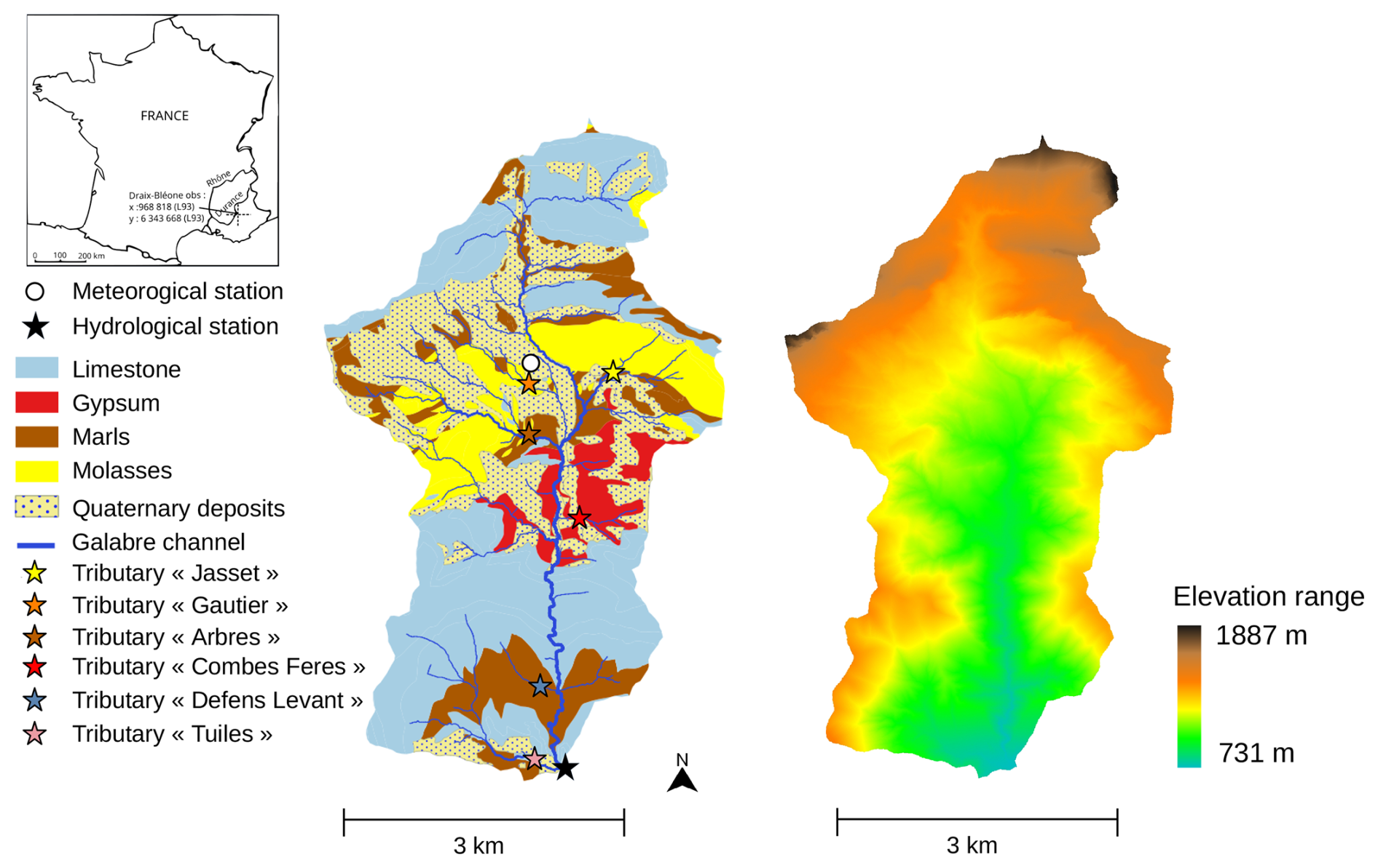
Figure 1 Lithological and elevation maps of the Galabre catchment. The different sampled tributaries during spatial campaigns are shown with colored stars.

The climate is both Mediterranean and mountainous, characterized by frost in winter and high temperature in summer. Mean annual rainfall and SS export is 792 mm and 660 Mg km⁻² yr⁻¹ (Legout et al., 2021). Spring/summer (from May to September) is a dry season with low flow rate values (Fig. 2a) but subject to short duration (1–2 h) and high-intensity rainfalls (Fig. 2b), that lead to events with high SSC (Fig. 2d). Autumn/winter (from October to April) is characterized by long duration (> 5 h) and low-intensity rainfalls (Fig. 2b), leading to high hydrological connectivity, higher flow rate values (Fig. 2a) and lower SSC values (Fig. 2d). Both seasons show considerable SS export (Fig. 2e) (Esteves et al., 2019; Navratil et al., 2012; Legout et al., 2021).

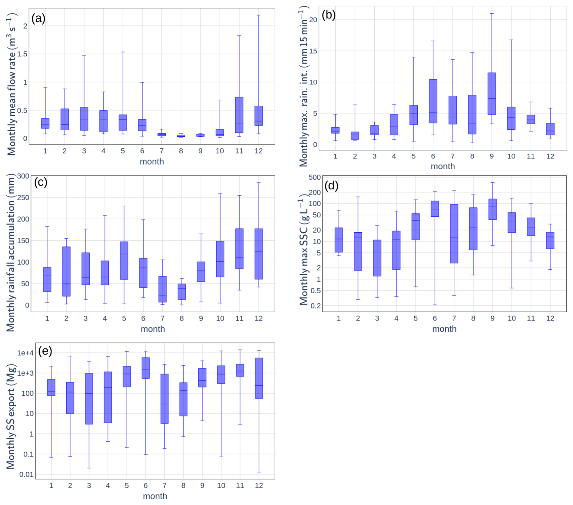
Figure 2 Seasonal variations of (a) monthly mean flow rate, (b) monthly maximum rainfall intensity, (c) monthly rainfall accumulation, (d) monthly maximum suspended sediment concentration (SSC) and (e) monthly suspended export (SS) export in the Galabre catchment, computed with data taken at the Galabre outlet and the meteorological station from 2007 to 2025.

The lithology of the Galabre catchment comprises limestones (34 %), marls and marly limestones (30 %), gypsum (9 %), molasses (9 %), and Quaternary deposits (18 %) (Esteves et al., 2019; Legout et al., 2021). Unvegetated badland areas occupy approximately 9.5 % of the catchment surface and are spatially dispersed throughout the catchment. The badlands, developed in marls and molasses lithologies, constitute the dominant source of SS exported at the catchment outlet (Legout et al., 2013).

The mean slopes are approximately 54 % for hillslopes, 19 % for intermittent tributaries, and 6 % for the main river channel (Legout et al., 2021). The land cover is dominated by forests (52 %), scrubland (30 %), sparse vegetation (12 %), and grasslands (3 %) (Esteves et al., 2019), with small agricultural and urban areas located in the lower part of the catchment. Some parts of the catchment are covered by thin soil, less than 0.5 m deep (Esteves et al., 2019; Legout et al., 2021). Given the steep topography and high rainfall intensities, infiltration-excess overland flow is assumed to be the dominant SR generation mechanism, consistent with observations from other Mediterranean badland catchments (Nadal-Romero et al., 2008b; Cantón et al., 2001; Romero-Díaz et al., 1999).

3 Data and methods

3.1 Data acquisition

The datasets collected in the Galabre catchment are detailed in Legout et al. (2021) and include the following:

• -

  Meteorological data from a local weather station (white point in Fig. 1), including 15 min time step rainfall records from 2019 to 2025 obtained using a 0.2 mm resolution tipping-bucket rain gauge.

• -

  Continuous measurements of flow rate and SSC from 2019 to 2025 at a 10 min time step at the hydrological station (black star on Fig. 1).

• -

  Concentrations of metals and trace elements in 667 water samples collected at different places in the catchment between April 2022 and June 2025, comprising:

  • -

    579 samples collected at the hydrological station (black star on Fig. 1) using automatic sequential samplers, with variable time steps (ranging from approximately 0.5 to 3 h) determined according to turbidity and water level variability. Weekly samples are also collected throughout the year.

  • -

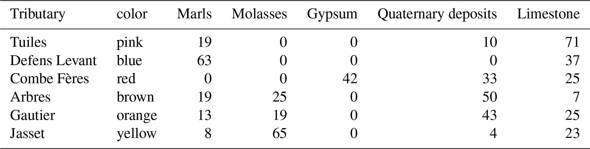
    10 spatial sampling campaigns conducted under baseflow conditions between February 2023 and May 2025, during which metal and trace element concentrations were measured in six Galabre tributaries (locations indicated by stars in Fig. 1 and summarized in Table 1).

  • -

    28 measurements of metal and trace element concentrations in water samples collected in surface runoff collectors installed on marl and gypsum hillslopes, from November 2023 to June 2025.

Table 1 Contribution of each lithology to the contributing area of each sampled tributaries, in %. Colors correspond to the stars' colors on Fig. 1.

For chemical measurements, water samples were collected in the field, and brought to the lab. Each sample was then filtered at 0.2 µm with acetate cellulose syringe filters (Minisart NML, Sartorius), diluted by a factor of 10 with ultrapure water, and acidified at a volumetric concentration of 2 % of HNO₃. Dissolved concentrations of 47 elements were analyzed in each sample, using Inductively Coupled Plasma - Mass Spectrometer (ThermoFisher Scientific ICP-MS iCAP TQ, with ESI SC4DX automatic sampler and FAST valve injection). Concentration quantifications were conducted using external calibrations performed with authentic elemental standard solutions prepared once a week, using seven calibration standards with known elemental concentrations covering the concentration range typically encountered in continental waters. Internal standards (In, Re, Ir, Tl) were used to correct from instrumental drift and potential ionisation variations due to matrix effect. Analytical reproducibility and accuracy were verified using homemade mixed standard solutions, and certified solutions (CMS-5 and IV-STOCK50 from Analab), respectively. Procedural and analytical errors are lower than 10 % for elemental concentrations. Limits of quantification are below 1 µg L⁻¹ for Li, Ti and Sr; and below 20 µg L⁻¹ for Na, Si, S and Ca.

This very rich chemical dataset makes the Galabre catchment an interesting area to perform hydrograph decomposition and study the respective role of GW and SR in erosion processes.

3.2 Chemical-based hydrograph decomposition method

The End-Member Mixing Analysis (EMMA) framework was developed through the selection of conservative chemical tracers, identification of distinct end-members (EM), and characterization of their chemical signatures (Christophersen et al., 1990; Christophersen and Hooper, 1992; Pinder and Jones, 1969; Hooper, 2001). EMMA assumes conservation of tracer mass and water within the catchment, expressed as by Eq. (1) (Christophersen et al., 1990):

$$\begin{array}{}\text{(1)}& \left\{\begin{array}{l}\sum C_{s,i}{\mathit{\alpha }}_i=C_s,\\ \sum {\mathit{\alpha }}_i=\mathrm{1},\end{array}\right.\end{array}$$

where C_s,i is the concentration of tracer s in EM i, α_i the proportional contribution of EM i, and C_s the tracer concentration in the total flow. For a system with n EM, at least n − 1 tracers are required to resolve Eq. (1).

3.2.1 Sampling of potential end-members

GW chemistry was characterized using the ten spatial sampling campaigns conducted in Galabre tributaries during low-flow periods to capture spatial and seasonal GW variability of water chemistry across lithologies. SR chemistry and its temporal variability throughout the year were characterized from the 22 samples collected by the two surface runoff collectors installed in the catchment.

3.2.2 Normalization and Principal Component Analysis (PCA)

All element concentrations were normalized using the mean and standard deviation of outlet data to ensure comparability. PCA was then applied to outlet concentrations to reduce dimensionality and define the main axes of chemical variability (Christophersen and Hooper, 1992; Hooper, 2003). Source samples were projected into this PCA space to visualize mixing patterns.

3.2.3 Tracer and end-member selection

Only chemodynamic and conservative tracers were retained, based on solute–solute relationships (R² > 0.5, p_value < 0.01) (Barthold et al., 2011; Birkel et al., 2021; Inamdar et al., 2013; Iwasaki et al., 2015) and range tests ensuring stream concentrations are bounded by EM concentration (Iwasaki et al., 2015). PCA space was then used to select the tracer combination that provides the best separation of sources in the PCA space. The number of EM was determined from the Rule of One (Iwasaki et al., 2015) and the residual diagnostic test of Hooper (2003) (Barthold et al., 2011; Birkel et al., 2021; James and Roulet, 2006; Iwasaki et al., 2015; Liu et al., 2017). EM were defined as groups of one or more sources, outlining a convex polygon in PCA space enclosing the outlet chemistry.

3.2.4 Temporal and spatial variability of EM chemistry

Low-flow conditions are typically associated with older groundwater flows, which exhibit higher solute concentrations (Ortega et al., 2025). This study uses this general assumption to adapt the chemical composition of EM with flow rate. Decreasing exponential regressions between outlet flow rate (Q) and element concentrations in each tributary were used to adjust the chemistry of each tributary according to pre-event flow. Only regressions with a coefficient of determination R² > 0.5 were retained. For weaker relations (R² < 0.5), mean concentrations in the tributary across all spatial campaigns were used. The chemical composition of EM was then defined as the mean of the tributary concentrations within each EM group, whether derived from the decreasing exponential regressions or from a simple averaging. Uncertainties in tracer concentrations for each tributary were quantified as the maximum observed deviation between the adjusted (or averaged) value and the measured concentrations across all spatial campaigns.

3.2.5 EMMA model solving and evaluation

The EMMA equations (Eq. 1) are solved using a mass balance approach. Several solution methods were implemented to assess the relevance of adapting EM concentrations to the hydrological state of the catchment using the exponential recession relationships described in Sect. 3.2.4. These methods are presented in Appendix A.

Uncertainties were estimated by a 10 000 iteration Monte Carlo simulation, randomly sampling tracer concentrations from normal distributions around the defined uncertainty on EM chemistry, computed based on the uncertainty on tributary chemistry (Foster et al., 2001; Ribolzi et al., 2000). Model performance was evaluated by: (i) verifying that SR contributions approached zero during baseflow periods; (ii) testing model accuracy using virtual mixtures, (iii) application of the different EMMA models to samples collected at the catchment outlet during the spatial campaigns, using the concentrations measured during each spatial campaign to define EM chemistry. This allowed for comparison of the EM contribution estimates obtained using: (i) the exact EM compositions (measurements during the spatial campaign), (ii) the EM compositions based on the mean values, and (iii) the EM compositions estimated with the decreasing exponential regression between the outlet flow rate and element concentrations.

3.3 Interpolation of the surface runoff rate with the filtering method during rainfall–runoff events

Rainfall–runoff events were defined as periods during which SS flux exceeded 0.2 kg s⁻¹. An event was considered to terminate once flow rate declined below one-seventh of the event's peak flow rate. To enhance the temporal resolution of hydrograph decomposition performed with the EMMA method during rainfall–runoff events, an Eckhardt recursive filter (Eckhardt, 2005) was applied to single-peak events with at least four chemical measurements that correspond to 30 events. This two-parameter filter separates total flow rate into GW and SR components using Eq. (2):

$$\begin{array}{}\text{(2)}& \begin{array}{l}{Q}_{\mathrm{GW},\mathrm{0}}=Q_{\mathrm{0}},\\ Q_{\mathrm{GW},i}={\displaystyle \frac{\left(\mathrm{1}-{\text{BFI}}_{max}\right)\mathit{\alpha }{Q}_{\mathrm{GW},i-\mathrm{1}}+(\mathrm{1}-\mathit{\alpha }){\text{BFI}}_{max}{Q}_i}{\mathrm{1}-\mathit{\alpha }{\text{BFI}}_{max}}},\end{array}\end{array}$$

where Q_GW,i and Q_i are the GW and total flow rates at time step i, and α and BFI_max are filter parameters. These parameters were calibrated for each rainfall–runoff event by minimizing the difference between GW estimates from the EMMA model and from the filter (Zhang et al., 2013; Andermann et al., 2012). After calibration, only events with a relative root mean squared error below 0.5 between the two GW estimates, and with a maximum SR rate estimate superior to 0.05 m³ s⁻¹ were retained, which corresponds to 26 events. It has been checked that this 26-event subset falls within the overall distributions of event characteristics observed since 2008 in the Galabre catchment.

For these selected events, several hydrological and sedimentary indicators were computed at the event scale, including: maximum rainfall intensity (I_max, mm 15 min⁻¹), total rainfall (P_tot, mm), 15 d antecedent rainfall (P₁₅, mm; 15 d duration chosen after preliminary sensitivity tests), event duration (hours), maximum flow rate (Q_max, m³ s⁻¹), maximum SR flow rate (Q_SR,max, m³ s⁻¹), maximum GW flow rate (Q_GW,max, m³ s⁻¹), percentage of SR at peak flow (%SR, pkf, %), flow export (V, m³), SR export (V_SR, m³), GW export (V_GW, m³), percentage of volume of SR relative to total flow export (%V_SR, %), maximum SSC (SSC_max, g L⁻¹) and SS export (V_s, t). Pearson correlations are computed to test for relations between rainfall, hydrological, and sedimentary characteristics of these events. The p_value associated with each correlation is calculated, testing the null hypothesis of no linear correlation between the variables. Only correlations with p_value < 0.05 are kept.

3.4 Flow-suspended sediment relationships analysis and hysteresis index calculation

The flow SS relationship was analyzed with the well-known power function (Jing et al., 2025) :

$$\begin{array}{}\text{(3)}& {\displaystyle }Q=a_{\mathrm{tot}}{\text{SSC}}^{b_{\mathrm{tot}}}\text{(4)}& {\displaystyle }{Q}_{\mathrm{SR}}=a_{\mathrm{SR}}{\text{SSC}}^{b_{\mathrm{SR}}}\end{array}$$

The a coefficient is often associated with SS availability, whereas the b coefficient is interpreted in terms of river transport capacity (Jing et al., 2025; Asselman, 1999)

The normalized hysteresis index (HI) proposed by Lloyd et al. (2016) was used to characterize the shape of event SSC–Q hysteresis loops. Only single-peak events were kept for the analysis for the HI index.

4 Results

4.1 Construction of the EMMA models

The selected tracers for the EMMA model were Li, Na⁺, Si, S, Ca²⁺, Ti, Sr.

Figure 3 shows that the sampled water sources cluster into four distinct EM. Although the primary objective of the study is to isolate the SR contribution, Fig. 3 shows that the spatial variability in GW chemistry requires the consideration of multiple GW EMs, which are necessary to encompass the range of streamwater measurements:

• Surface runoff end-member (EM_SR): represented by surface runoff collector measurements (black), corresponding to surface runoff.

• Groundwater end-members (EM_GW): comprising three distinct types, each associated with different tributaries, draining different lithologies:

  • Evaporite EM: associated with the gypsum-rich tributary (tributary Combe Fères), characterized by high concentrations of S, Ca²⁺, Li, Ti, and Sr (see Table 2).

  • Sedimentary EM: corresponding to tributaries draining marl, limestone, and molasse formations (tributaries Jasset, Tuiles and Defens Levant).

  • Quaternary EM: associated with tributaries in the upstream part of the catchment, primarily draining Quaternary deposits, and characterized by elevated concentrations of Na⁺ (tributaries Arbres and Gautier).

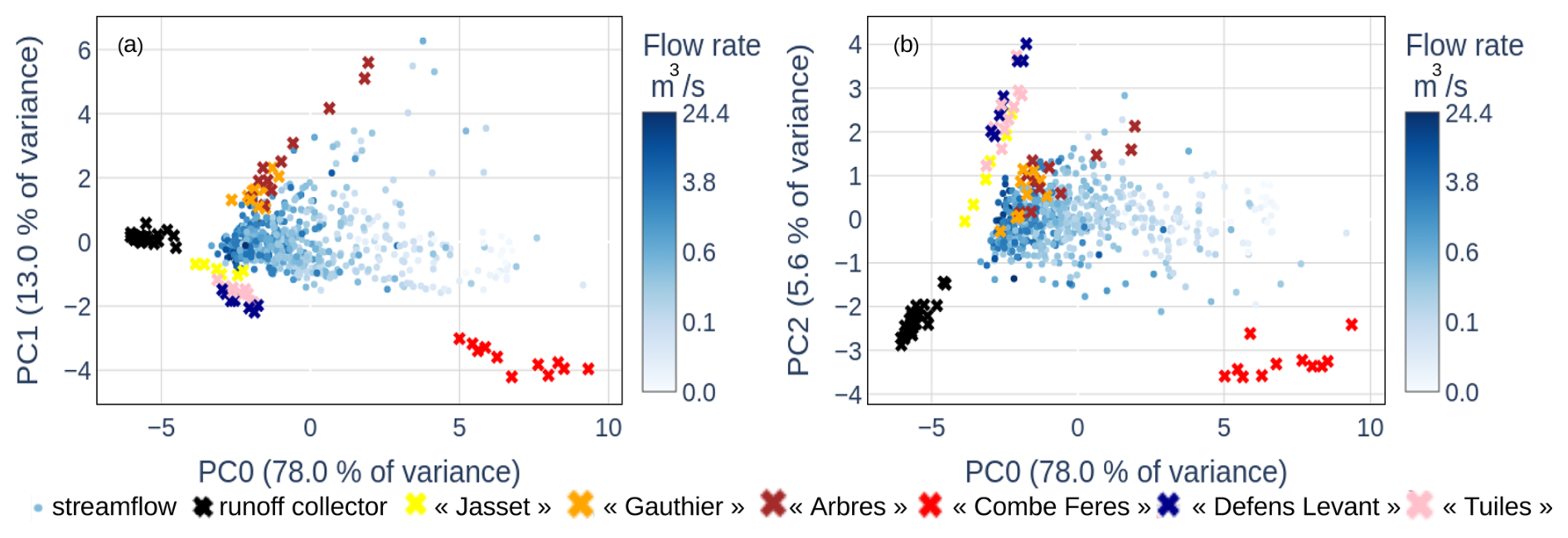
Figure 3 Results of the Principal Component Analysis (PCA) performed with streamwater samples (blue points, with outlet flow rate represented by the color scale). Source samples (cross symbols) are projected onto this PCA space: black crosses represent measurements from the surface runoff collectors, while other colored crosses correspond to tributary sources. Each color corresponds to a tributary, with the same colors of the crosses used in the Galabre map in Fig. 1 and Table 1. Multiple points with the same color indicate different sampling campaigns conducted within the same tributary. The association of colors to the different geologies and end-members is: evaporite rocks (red), sedimentary rocks (yellow, pink, blue) and quaternary rocks (orange, brown), surface runoff (black).

Table 2 Loadings of the three first principal components of the Principal Component Analysis computed with the chemical measurements of the 579 samples taken at the Galabre outlet.

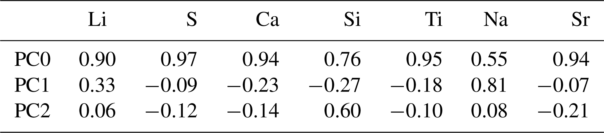
The use of these four EM satisfies the diagnostic criteria proposed by Hooper (2003) and the “Rule of One”. Figure 3 indicates that the chemical composition of EM_SR shows limited spatial and temporal variability. In contrast, the EM_GW display significant spatial variability, evidenced by differences in chemical composition among tributaries within the same EM, and temporal variability, as the chemistry of individual tributaries changes between the time of the different spatial campaigns.

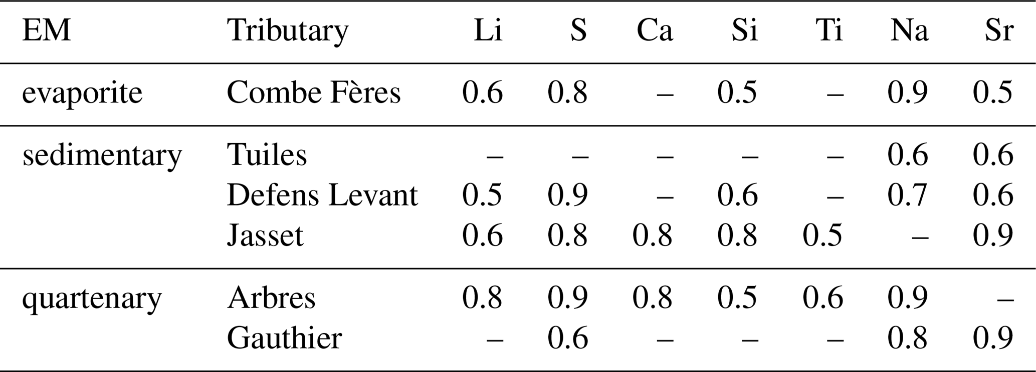
Table 3 shows that for some chemical elements and some tributaries (27 among the 42 couples of element-tributary), this chemical temporal variability can be partly explained by a decreasing exponential function with flow rate at the catchment outlet. A graphic representation of these relationships for one tributary is given in Sect. A1 of Appendix A. These exponential relationships were used to adjust the chemical composition of the tributary sources for each event, using the pre-event flow rate value at the catchment outlet.

Table 3 Coefficient of determination of the exponential fit between tracer concentrations and flow rate at the catchment outlet during spatial campaigns, keeping only relations with R² > 0.5.

Tests and evaluations of the different EMMA models are presented in Appendix A. These analyses show that adapting EM_GW chemistry to the hydrological state of the catchment provides more accurate estimates of streamflow source contributions, both during and outside rainfall–runoff events. Results also show that this approach reduces the uncertainty associated with SR contribution estimates. Based on these results, only the outputs of the EMMA model adapting EM chemistry to the hydrological state of the catchment are analyzed in the subsequent sections of this study. Based on the Monte Carlo analysis and the evaluation of this EMMA model performance under low-flow conditions, presented in Appendix A, the uncertainty associated with SR contribution was estimated around 15 %.

4.2 Hydrological characteristics of the rainfall runoff events

Figure 4a shows the result of the hydrograph decomposition and highlights in particular that the contributions of the surface runoff EM rise with flow rate. Figure 4b indicates that SR contributions vary between 0 % and 50 % during rainfall–runoff events, and that the relationship between flow rate and SR contribution is highly dispersed throughout the year. Figure 4c and d highlight seasonal trends in both SR and GW flow rates, with low values between May and September, and higher values in winter, from October to April. These observations led us to divide the event dataset in two distinct periods, associated with different hydrosedimentary characteristics (see Table 4). Table 4 shows that from May to September, events (named spring/summer events) are characterized by low duration events, high maximum rainfall intensities, low rainfall accumulation, low maximum flow rate, low maximum SR and GW flow rate, low SR and GW exports, high maximum SSC and low SS export. From October to April, events (named autumn/winter events) are characterized by higher duration events, lower rainfall intensities, higher rainfall accumulation, higher maximum flow rate, higher maximum SR and GW flow rate, higher SR and GW export, lower maximum SSC and higher SS export. Table 4 also shows that, during both seasons, GW is the main contributor of water, representing around 70 % of flow rate at peak flow and around 75 % of water flow at event scale.

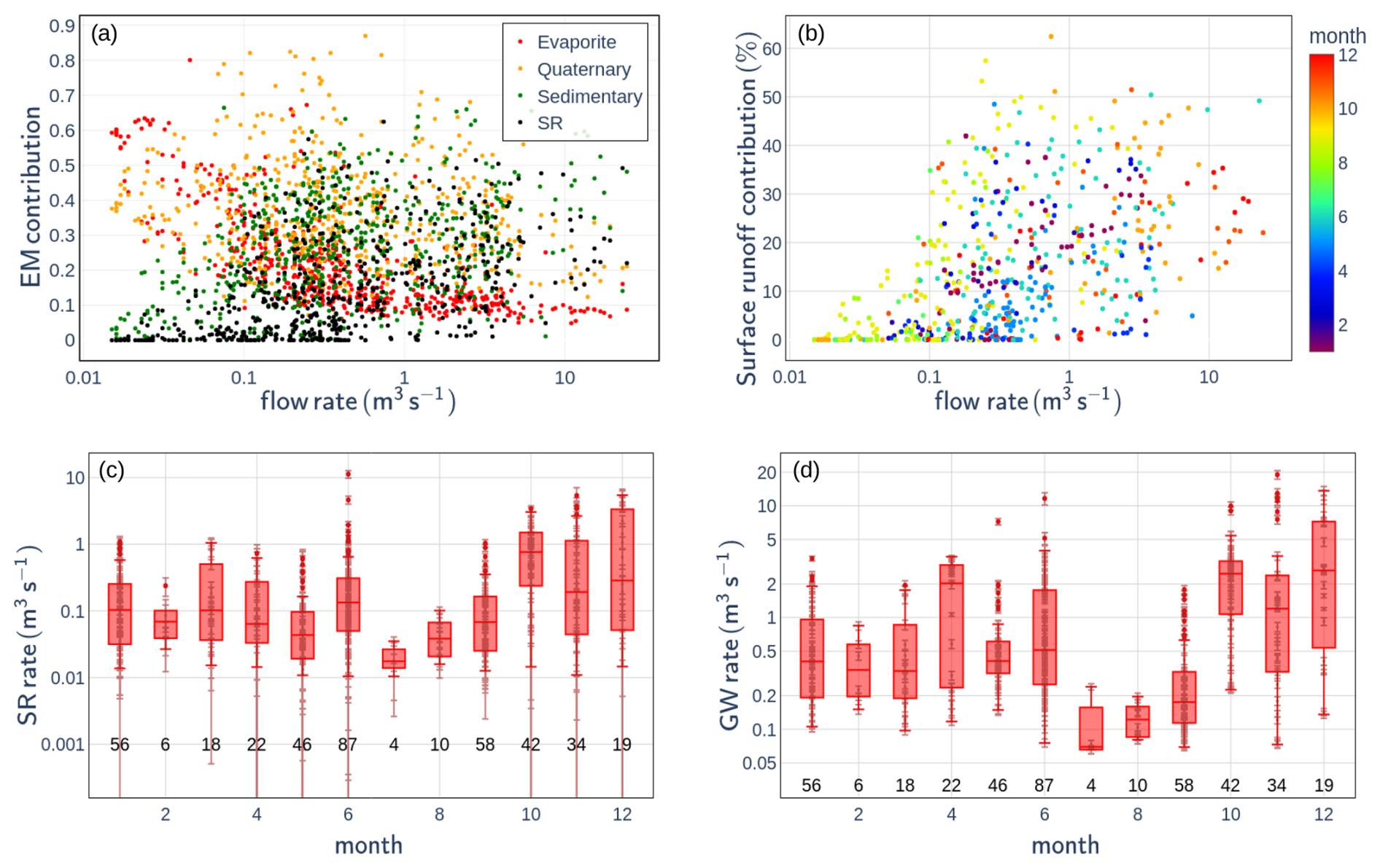
Figure 4 (a) Contributions of the different end-members (EM) as a function of flow rate at the Galabre outlet; (b) surface runoff contribution to total flow at the outlet as a function of flow rate, with points colored by month; (c, d) surface runoff (SR) flow rate and groundwater (GW) flow rate, respectively, at the Galabre outlet during rainfall–runoff events, shown by month. The number of samples per month is indicated above the x axis.

Table 4 Minimum, maximum, and average values of various hydrosedimentary indicators by season, computed for 26 events (10 in spring–summer and 16 in autumn–winter) using high-frequency hydrograph decompositions obtained with the Eckhardt filter.

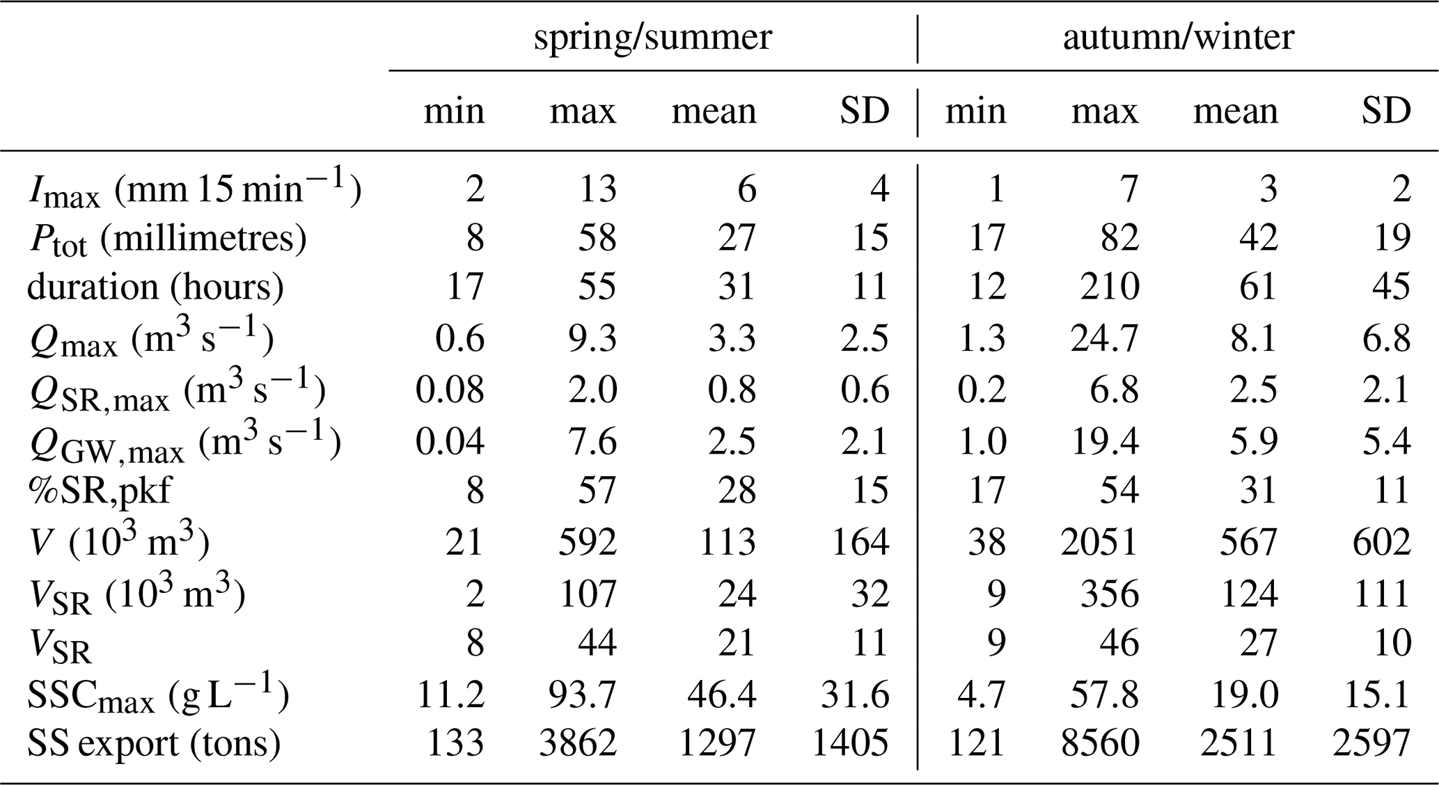
Table 5 indicates that key hydrological variables, including Q_max, Q_SR,max, Q_GW,max, V, V_SR, V_GW are strongly correlated with event rainfall accumulation P_tot and 15 d antecedent rainfall accumulation (P₁₅). Additionally, surface runoff-related variables (Q_SR,max, V_SR) show higher correlations with P_tot, and groundwater-related variables (Q_GW,max, V_GW) show higher correlations with 15 d antecedent rainfall accumulation (P₁₅) than variables related to surface runoff (Q_SR,max, V_SR). Table 5 also indicates that Q_max and V are highly correlated to Q_GW,max and V_GW respectively.

Table 5 Pearson correlation coefficients between hydrological and sedimentary variables, computed for all the 26 events, using the high-frequency hydrograph decomposition interpolated with the Eckhardt filter. Only relations with p_value < 0.05 are kept. The table is presented in a reduced non-symmetric form.

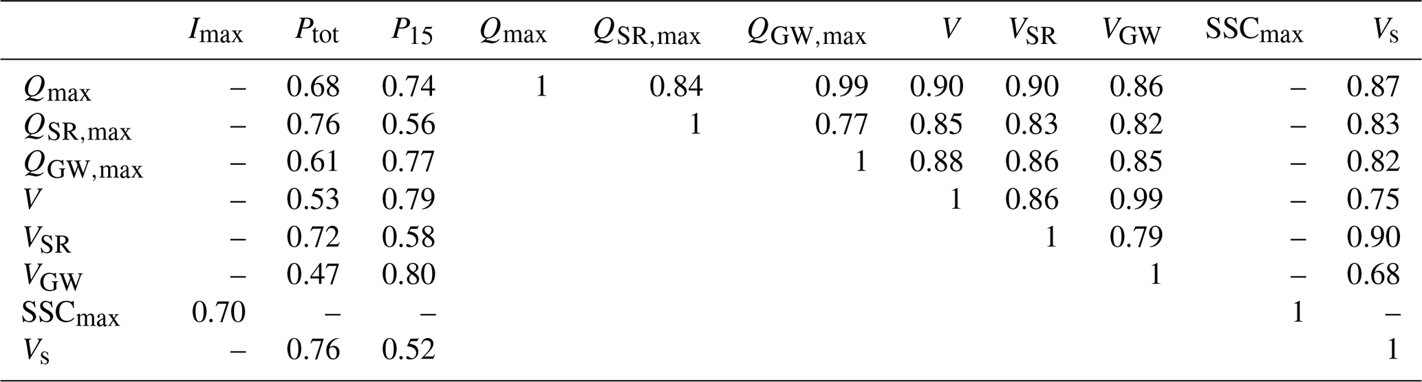
Table 6 Pearson correlation coefficients between hydrological and sedimentary variables, computed for the 16 events occurring from October to April, using the high-frequency hydrograph decomposition interpolated with the Eckhardt filter. Only relations with p_value < 0.05 are kept. In spring/summer, the equivalent calculation on the 10 available events shows only one significant correlation of 0.69 between I_max and SSC_max.

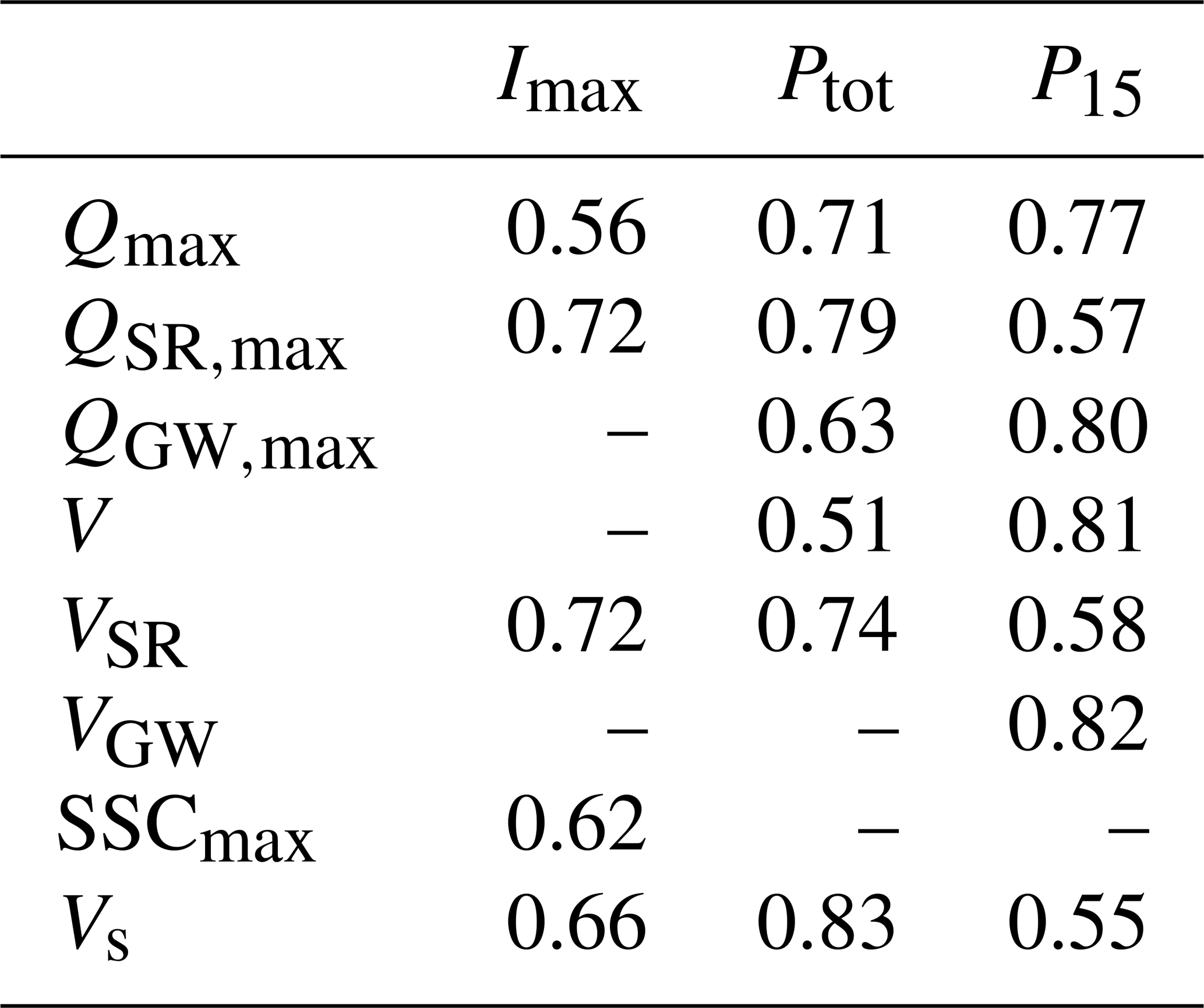
Results presented in Table 6 highlight a marked seasonal contrast in the influence of rainfall characteristics on hydrological responses. During autumn/winter, most of the hydrological variables are correlated with event rainfall characteristics. Surface runoff related variables are highly related to I_max, whereas groundwater-related variables show stronger correlations with P₁₅. In contrast, during spring/summer, no significant correlations are observed between hydrological responses and either rainfall intensity or cumulative rainfall.

This seasonal disparity is further illustrated in Fig. 5a, which shows a clear relationship between Q_SR,max and I_max during autumn/winter period events, whereas this relationship is not evident during spring/summer events.

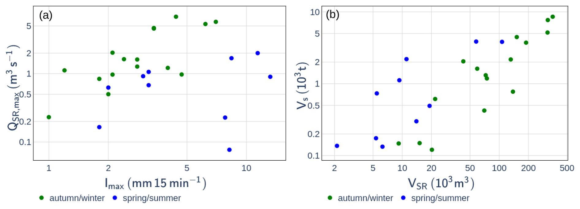
Figure 5 Relations between (a) event maximum rainfall intensity I_max and maximum surface runoff flow rate Q_SR,max; (b) exported surface runoff volume (V_SR) and suspended sediment export V_s. Each point represents one of the 26 events interpolated with the Eckhardt filter calibrated with the results of the End Member Mixing Analysis method.

4.3 Relation between suspended sediment concentration and flow rate

Figure 6a and Table 7 show that the relationship between instantaneous SSC and Q at the catchment outlet is highly scattered, as indicated by a low Pearson correlation coefficient. Part of this variability can be attributed to seasonal differences: for a given flow rate, higher SSC values are generally observed in summer compared to autumn/winter. This seasonal effect is further supported by higher Pearson correlation coefficient when the dataset is divided by season, as shown in Table 7.

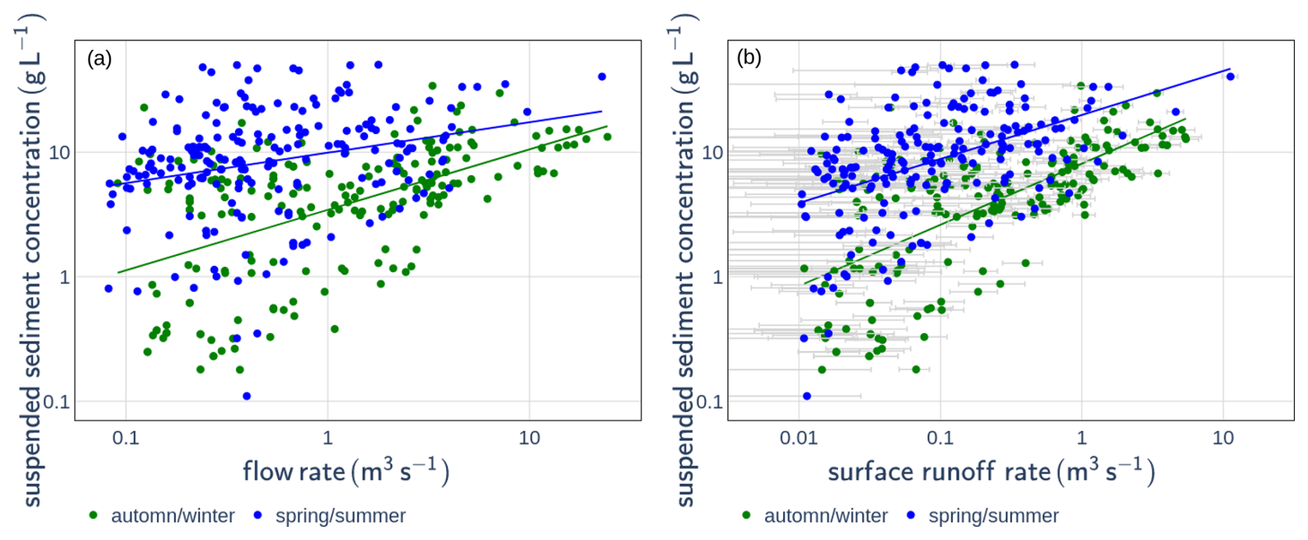
Figure 6 Relationship between suspended sediment concentration and (a) total flow rate or (b) surface runoff flow rate, distinguished by season: October–April (green) and May–September (blue). Light-grey uncertainty bars represent uncertainties associated with the End Member Mixing Analysis results.

Table 7 Parameters a, b, and the Pearson coefficient (r) of the tested rating curves (see Eqs. 3 and 4). All relationships have a p_value < 0.05.

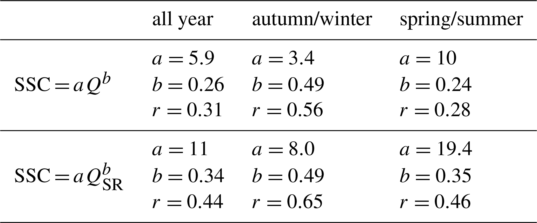
Table 7 also demonstrates that SSC correlates more strongly with Q_SR than with Q, both for the complete dataset and within each season, as evidenced by higher Pearson correlation coefficients. This is particularly pronounced during the spring/summer period. Despite this reduction in scatter, Fig. 6b shows that the SSC–Q_SR relationship still exhibits considerable variability and retains a clear seasonal signal. Additionally, Table 7 reveals that in both the SSC–Q and SSC–Q_SR power-law relationships, the coefficient a is considerably larger in spring/summer than in autumn/winter.

At the event scale, Table 5 shows that event SSC_max is only correlated with I_max, whereas V_s is significantly correlated with P_tot and all other hydrological variables (Q_max, Q_SR,max, Q_GW,max, V, V_SR, and V_GW). Table 5 also shows that V_s correlates more strongly with SR-related variables (Q_SR,max, V_SR) than with GW-related variables (Q_GW,max, V_GW). Figure 5b suggests that the persistent variability in the relationship between V_SR and V_s can be partly explained by seasonal effects, with higher sediment exports observed in spring/summer compared to autumn/winter for a given V_SR.

Table 6 shows that, similar to hydrological variables, V_s is strongly correlated with rainfall intensity and accumulation in autumn/winter, but not in spring/summer. However, SSC_max and I_max are significantly correlated during both seasons.

The hysteresis index (HI) of the relationship between SSC and Q was calculated for all single peak events between October 2019 and June 2025, which represent 86 events (Fig. 7). Among these events, 19 show eight or complex hysteresis shapes, 34 show anti-clockwise hysteresis shapes, and 33 show clockwise hysteresis shapes. Only the events associated with clockwise and anti-clockwise loops were kept for the following analysis. Among these 67 events, 19 events were covered by high-frequency hydrograph decomposition interpolated with the Eckhardt filter.

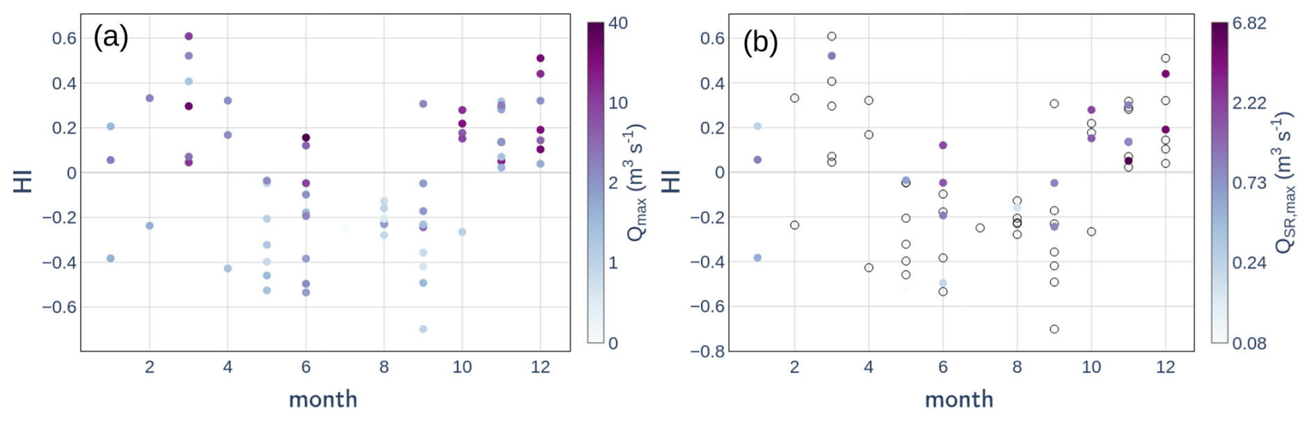
Figure 7 Monthly variation of hysteresis index (HI) of events associated with clockwise and anti-clockwise loops from October 2019 to June 2025, with color representing: (a) event maximum flow rate (Q_max), (b) event maximum interpolated surface runoff flow rate (Q_SR,max). Transparent points on panel (b) are events for which interpolation of surface runoff flow rate with Eckhardt filter is not available.

Figure 7 indicates a seasonal shift in HI sign, with a transition from negative HI between May and September, characterized by SSC peaks occurring after the Q peaks (i.e., anticlockwise hysteresis), to positive HI values from October to April, where SSC peaks precede Q peaks (i.e., clockwise hysteresis).

5 Discussion

The wealth of available data, combined with the development of original analytical methods, provided new insights into hydro-sedimentary processes within medium-scale Mediterranean catchments. First, an EMMA approach was developed to adjust end-member chemical signatures according to the catchment's hydrological state, thereby accounting for variations in groundwater age (Rademacher et al., 2005; Ortega et al., 2025). Second, this method was applied to an extensive chemical dataset comprising 579 samples collected over multiple hydrological years and seasons. Finally, the chemically based hydrograph separations were used to calibrate the Eckhardt filter at the event scale, enabling high-frequency hydrograph decomposition for 26 events.

5.1 Hydrological processes in the catchment

The correlations between P_tot and both Q_SR,max and Q_GW,max, especially from October to April (Table 6) suggest that the seasonal variability of SR and GW flow rates (Fig. 4c, d) likely reflects the seasonal distribution of rainfall accumulation (Fig. 2c), with higher accumulations in winter and early spring compared to summer. However, the lack of significant correlation between Q_SR,max and I_max in spring/summer likely reflects the highly intense and localized nature of spring/summer rainfall events that are not homogeneously spread all over the catchment. While high-intensity rainfall is generally expected to enhance SR production, as documented in other small-scale badland catchments (Nadal-Romero et al., 2008a; Cantón et al., 2001; Romero-Díaz et al., 1999), the spatial averaging of the measurement at the 20 km² catchment outlet may obscure this relationship. In contrast, autumn/winter rainfall events are typically less intense and more spatially uniform (Navratil et al., 2012). The wet soils at this period are more hydrologically connected (Hachgenei et al., 2024; Kaffas et al., 2025), and this leads to significant correlations between rainfall intensity and hydrological responses.

The relatively scattered relationship between rainfall characteristics and SR production, even in autumn/winter (Fig. 5a), may also result from the integration of contrasting hydrological responses across the catchment: flashy SR responses from badland areas (Nadal-Romero et al., 2008a; Cantón et al., 2001; Romero-Díaz et al., 1999; Ribolzi et al., 2000) versus more attenuated responses from vegetated areas, influenced by pre-event hydrological conditions (Nadal-Romero et al., 2008a; Garcıa-Ruiz et al., 2005; Lana-Renault et al., 2007; Gallart et al., 2002). This spatial integration of various land cover could also likely explain the lower SR contribution observed in the medium-scale Galabre catchment compared to the much higher SR contributions (up to 80 %) reported in a nearby headwater catchment with approximately 80 % badland cover (Cras et al., 2007).

The high proportion of GW flow (around 75 % at the event scale, see Table 4) associated with the very high correlation between hydrological variables (Q_max, V) and GW-related variables (Q_GW,max, V_GW) indicate that the flow rate variabilities are mainly governed by the GW flow variabilities. This GW flow signal is partly decorrelated to the rainfall signal due to complex hydrological processes involving evapotranspiration, which exhibits strong seasonal dynamics. This high contribution of GW flow is consistent with other estimations done in other small- and medium-scale mountainous catchments (Trust et al., 2025; Baraer et al., 2015; Ribolzi et al., 2000), but is much higher than GW contributions reported in a nearby headwater catchment (1 km²) with approximately 80 % badland cover (Fischer et al., 2026). Correlations between GW-related variables and 15 d rainfall accumulation suggest that GW dynamics are influenced primarily by long-term (weeks to months) changes in catchment hydrological connectivity, whereas SR response dynamics are dominated by short-term events (hours), with negligible memory effects.

These findings highlight that, at larger catchment scales, hydrological and sedimentary processes are increasingly affected by spatial heterogeneity in rainfall, lithology, and land cover and GW contribution during rainfall–runoff events, complicating the interpretation of hydrological dynamics compared to small-scale catchments. This argues for increasing the density of hydrological observations within relatively homogeneous headwater sub-catchments (Sabathier et al., 2023; Uber et al., 2021; Assendelft and van Meerveld, 2025).

5.2 Hydrosedimentary processes in the Galabre catchment

The correlation between SSC_max and I_max during both seasons (Table 5) highlights the key role of rainfall intensity in driving sediment detachment from hillslopes. Additionally, the stronger correlation between instantaneous SSC and Q_SR compared with Q (Table 7) is a notable finding, as it underscores the dominant role of SR in driving instantaneous SSC values. The dispersion decrease in the SSC–Q_SR relation is particularly pronounced in spring/summer, emphasizing the important role of SR in SSC dynamics during this season, likely through primary erosion on hillslopes. This critical influence of rainfall intensity and SR on sediment detachment and transport in badland environments has been documented in several previous studies (Nadal-Romero et al., 2008a; Cantón et al., 2001; Romero-Díaz et al., 1999; Gallart et al., 2005). These studies highlight the importance of bare areas and infiltration-excess SR in controlling sediment export dynamics.

However, the persistent scatter and seasonal variability observed in the SSC–Q_SR relationships suggest that SR flow alone cannot fully explain SSC dynamics. This shows that additional hydrosedimentary processes are involved, such as variability of sediment availability, transport capacity, or rainfall energy. The higher a coefficient in the power-law fits during spring/summer compared to autumn/winter for both SSC–Q and SSC–Q_SR relationships could indicate greater sediment availability in spring/summer compared to autumn/winter (Asselman, 1999; Jing et al., 2025). This pattern may result from progressive hillslope sediment depletion over the year or from seasonal differences in sediment sources (Gallart et al., 2005; Ariagno et al., 2023). Another notable point is the correlation between V_s and hydrological variables associated with both SR and GW (Table 5), indicating that GW inputs play a significant role in event-scale sediment transport. These last results, associated with the seasonal variations of hysteresis index (Fig. 7), allow the identification of two distinct seasonal periods, each characterized by contrasting hydrological and sedimentary behaviors (Fig. 8):

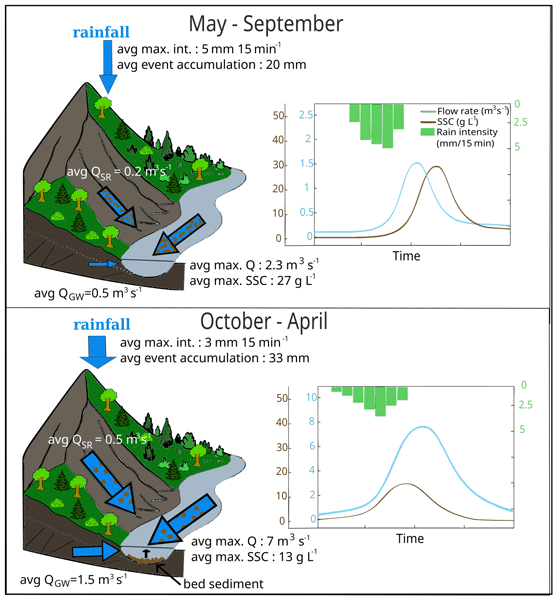
• May–September (hereafter referred to as spring/summer events): rainfall–runoff events during this period are characterized by high maximal rainfall intensities (average 6 mm 15 min⁻¹), short event durations (average 31 h), and low total rainfall accumulations (average 27 mm). The high rainfall intensities promote efficient sediment detachment from hillslopes, resulting in elevated SSC levels in SR flow. Dry pre-event hydrological conditions lead to low GW flow rate. Consequently, events during this period display relatively low maximum flow rate (average 3.3 m³ s⁻¹), low water exports (average 113 × 10³ m³), but high maximum SSC values (average 46 g L⁻¹). In these events, SSC peaks typically lag behind maximum flow rate, producing anticlockwise hysteresis patterns. This suggests that sediment export could be mainly driven by localized high-intensity rainfall over hillslope areas situated far from the catchment outlet. Moreover, velocity differences between sediment and flood wave propagation can favor anticlockwise hysteresis patterns when sediment sources are located far from the outlet. The combination of high SSC and low flow rate implies limited SS transport capacity, favoring sediment deposition in the hydrographic network during the falling limb of hydrographs. The high sediment availability during these events (reflected by the high a value in the SSC–Q and SSC–Q_SR power–law relationships, Table 3) likely results from the high SS stock in early summer. This high SS stock may result from the frost weathering process in winter (as observed in neighboring smaller catchments of the Draix Bléone observatory, Ariagno et al., 2023; Gallart et al., 2002) and the preferential export of very fine sediments in spring and summer up to exhaustion. This leaves mainly medium-scale particles available for transport during autumn and winter events (Ariagno et al., 2023). Among these exported sediments, very fine particles are flushed out of the catchment, while only medium-scale sediments may be temporarily deposited and stored in the riverbed during events.

• October–April (hereafter referred to as autumn/winter events): events occurring during this period are characterized by lower maximal rainfall intensities (average 3.0 mm 15 min⁻¹), longer durations (average 61 h), higher rainfall accumulations (average 42 mm), and substantial maximum GW flow (average 5.9 m³ s⁻¹; Fig. 4d). These conditions reflect higher antecedent hydrological connectivity and result in elevated event maximum flow rate (average 8.1 m³ s⁻¹) and higher flow export (average 567 × 10³ m³). Lower rainfall intensities induce reduced sediment detachment from hillslopes, and this combined to the high GW flow rates leads to lower SSC_max values. Nonetheless, these events are associated with substantial total sediment exports (average 1.3 ton), and HI analyses reveal a positive shift, indicating a change in dominant sediment sources. We hypothesize that, during autumn/winter events, increased flow rate enables the remobilization of sediments previously deposited during spring/summer events. This secondary source, located in the hydrographic network, is likely to be mobilized early in the event (Uber et al., 2021), leading to clockwise hysteresis patterns in which SSC peak precedes flow rate peak. Field observations support this interpretation with important fine sediment deposits observed in the riverbed during field campaigns at the end of spring/summer. Haddad et al. (2022) reported that deposited materials in the Galabre riverbed were, on average, four times coarser than SS. The lower a coefficient in the SSC–Q relationship during autumn/winter compared to spring/summer (Table 3) may therefore reflect the more difficult mobilization of this coarsest fraction of the SS stock during low-flow conditions, and/or the more efficient entrainment of slope-derived SS in summer due to higher rainfall intensities. This seasonal shift in sediment sources from hillslopes in spring/summer to riverbed during high flow periods in autumn/winter is consistent with findings by Grangeon et al. (2012), who observed an increase in SS particle size with increasing flow rate in the Galabre catchment.

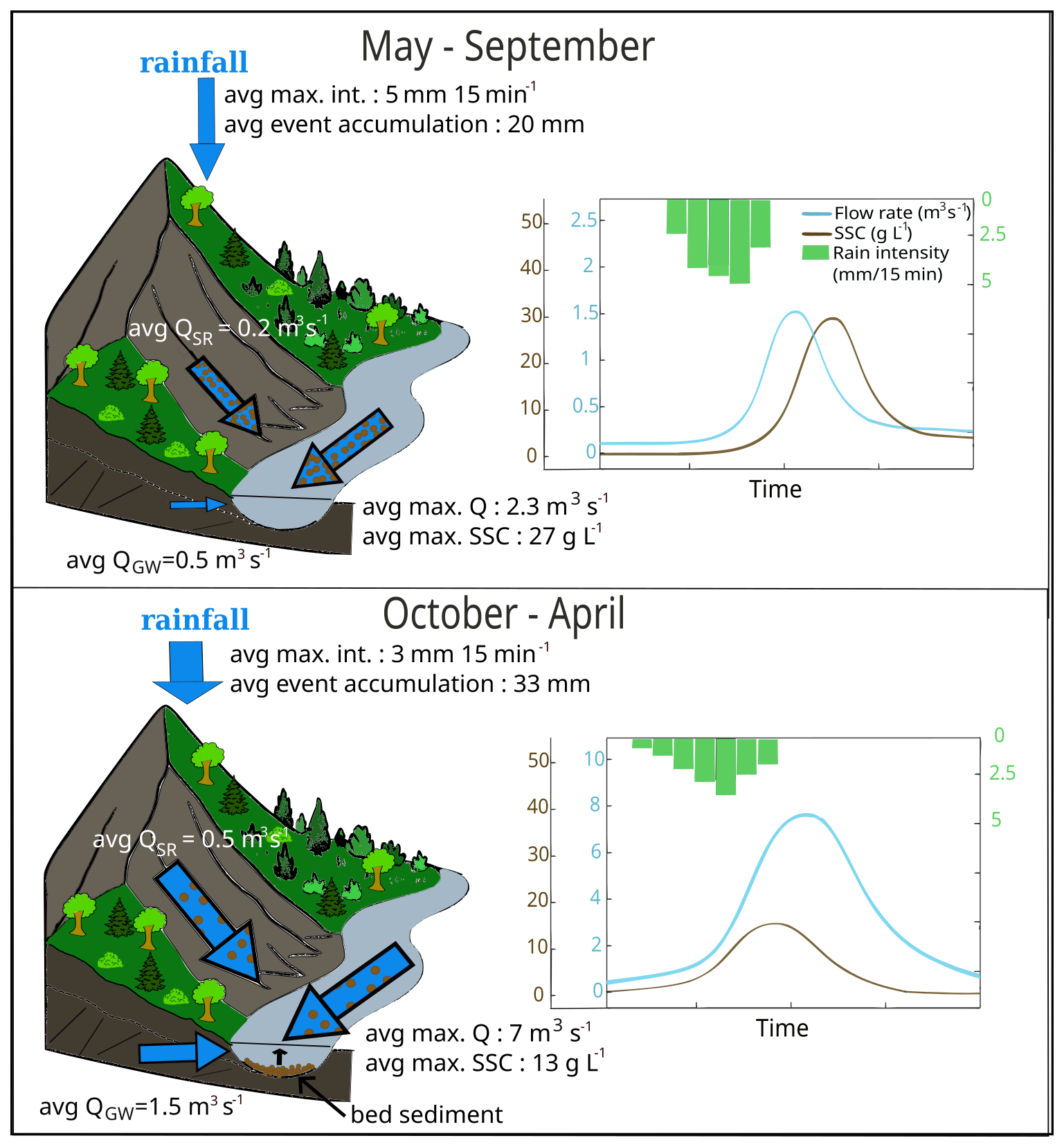
Figure 8 Conceptual diagram of the seasonal hydrosedimentary processes in the Galabre catchment.

This study highlights the critical role of GW input and of its temporal variability in shaping hydrosedimentary processes under Mediterranean climatic conditions. Low GW flows combined with localized high-intensity rainfall events in spring/summer promote intense sediment detachment from hillslopes and rapid deposition of the coarsest fraction among SS within the riverbed due to a limited transport capacity. In contrast, higher GW inputs during autumn/winter associated with long-duration rainfall events, generate events with high flow rates that facilitate the remobilization and export of these previously deposited materials. These results underscore the need to explicitly consider GW inputs and secondary erosion processes when studying SS export dynamics in Mediterranean catchments. These hypotheses of hydrosedimentary functioning in the Galabre catchment are consistent with the assumptions of Esteves et al. (2019): based on the analysis of SSC–Q relationships and hysteresis patterns from 2007 to 2014, Esteves et al. (2019) discussed the two contrasting seasonal regimes observed in June and November–December in terms of differences in rainfall intensity and river transport capacity during these periods. By quantifying SR and GW contributions, our study provides the next crucial quantitative step to clearly distinguish the underlying hydrosedimentary processes, and explain the seasonal functioning of the catchment.

5.3 River bed storage processes in a variety of catchments

Similar seasonal patterns of riverbed sediment deposition and subsequent remobilization have been reported in other Mediterranean and badland-dominated catchments (López-Tarazón et al., 2009; Navratil et al., 2010; Cantón et al., 2001; López-Tarazón et al., 2011). In a 445 km² Pyrenean catchment, where most sediments originate from badland areas, López-Tarazón et al. (2009) distinguished two main event types by analyzing event hysteresis patterns: (i) events with anticlockwise hysteresis, associated with intense rainfall localized over badland headwaters, resulting in high SR production but low SS export; and (ii) events with clockwise hysteresis, linked to more spatially uniform rainfall, characterized by lower SR flow rates but higher SS export. This hydrosedimentary behavior was attributed to the dual role of the riverbed of the hydrographic network, acting as a sediment sink in the first case and as a sediment source in the second. The same authors also highlighted the importance of GW inputs in the river system in maintaining non-zero SSC levels throughout the year. The riverbed sediment stock in this catchment was subsequently quantified by López-Tarazón et al. (2011), who showed that it can represent up to 65 % of the seasonal sediment load during autumn/winter, with a residence time shorter than 1 year. Similarly, Navratil et al. (2010) analyzed hysteresis patterns in the Bes River, a Mediterranean mountain river draining a 165 km² catchment that includes the Galabre catchment. Measurements of bed sediment storage over a 2.5 km reach revealed large sediment stocks comparable to suspended sediment inputs from upstream during events. They reported that approximately 80 % of the observed events exhibited clockwise hysteresis patterns, which they attributed to the remobilization of previously deposited riverbed sediments. Nadal-Romero et al. (2008b) investigated sediment dynamics in a 0.45 km² badland catchment in the Central Spanish Pyrenees. They associated clockwise hysteresis loops with wet antecedent conditions, long-duration rainfall, and strong hydrological and sediment responses. The rapid increase in SSC at the onset of events was attributed to the flushing of bed sediments, followed by a gradual decrease in SSC during the event, resulting from progressive dilution by GW inputs coming from vegetated headwaters. Conversely, anticlockwise hysteresis loops were linked to dry antecedent conditions, short and intense rainfall events, and moderate hydrological and sediment responses. During these conditions, SS were supposed to primarily come from badland areas, with sediment transport operating under a transport-limited regime and leading to sediment accumulation on hillslopes and intermittent hydrographic networks. The authors also emphasized that the apparent sediment exhaustion observed in SSC–Q relationships may not solely reflect source depletion, but can also result from progressive dilution by GW inputs as the hydrologically connected area becomes larger, particularly when vegetated zones become active contributors. Our study, conducted on a medium-scale catchment, shows that these seasonal patterns of sediment remobilization and deposition, particularly related to the role of the river as either a source or a sink of SS, are present across a wide range of catchment scales. These processes should therefore be accounted for in any modeling approach of SS fluxes, regardless of catchment size. To this end, spatially resolved observations of the seasonal dynamics of SS storage across the entire river network are required, potentially obtainable using drone-based LiDAR surveys. Alternatively, information constraining the age of sediments exported at the outlet is necessary to distinguish recently generated material (primary erosion) from older, remobilized deposits (Gourdin et al., 2014; Le Gall et al., 2017; Ribolzi et al., 2016).

6 Conclusions

This study provides an in-depth understanding of the hydro-sedimentary functioning of a medium-scale Mediterranean mountainous catchment, emphasizing the coupled roles of SR and GW flow rates in driving SS dynamics. The key methodological points developed in this study were (i) the development of an EMMA model that adjusts the chemical signatures of end-members according to the hydrological state of the catchment prior to each rainfall–runoff event, (ii) the application of this EMMA method on the very large and temporally detailed chemical dataset of the Galabre catchment, combining 580 chemical samples collected during 86 rainfall–runoff events, and (iii) the application of an Eckhardt filter on 27 rainfall–runoff events with filter parameters calibrated to minimize differences with EMMA GW estimates. This framework enabled a robust assessment of seasonal variability for SR and GW flow rates and their link with rainfall characteristics and SS export.

The analysis enables the identification of two distinct hydro-sedimentary regimes. Spring/summer regime (May–September) is dominated by short, intense rainfall events, associated with low flow, low maximum flow rate, high SSC peaks but low SS export, and anticlockwise hysteresis loops. These events were associated with hillslope-derived (primary erosion) sediment, transport-limited behavior, and deposition of SS in the riverbed of the hydrographic network. Autumn/winter regime (October–April) is characterized by lower intensity, long-duration rainfall events, high flow rate, high GW input, low SSC values, but high SS export, and clockwise hysteresis patterns. These events were associated with remobilization of previously deposited riverbed sediments in addition to the mobilization of remaining available particles on hillslopes.

This study underscores the fundamental role of GW input, representing around 75 % of event water flow. Its seasonal variability shapes both hydrological and hydrosedimentary seasonal functioning in this medium-scale Mediterranean catchment. Specifically, it drives sediment deposition during low-flow spring/summer periods and remobilization during high GW input in autumn/winter. The findings also emphasize the importance of separating GW and SR contributions before analyzing SS dynamics at the catchment outlet to avoid misinterpretation.

Appendix A: Tests and evaluation of the different EMMA methods

A1 Comparison of results from the three different EMMA methods

Three approaches were compared to solve the EMMA equations (see Eq. 1):

• MB_mean: mass balance solution using constant EM concentrations, computed as the mean over all the spatial campaigns (Ribolzi et al., 2000; Lukens et al., 2022).

• MB_fit: similar to MB_mean but using EM concentrations adjusted to the hydrological state of the catchment with the decreasing exponential regressions (see Sect. 3.2.4 and an example of adjustment in Fig. A1). Figure A1 further shows that incorporating this exponential fit between tracer concentration and outlet flow rate helps reduce uncertainty in defining the chemical concentrations of each tributary.

• MB_PCA,mean: solution in PCA space using projected EM signatures (Christophersen and Hooper, 1992; Iwasaki et al., 2015).

All models use a non-negative ridge regression constrained to ∑α_i = 1.

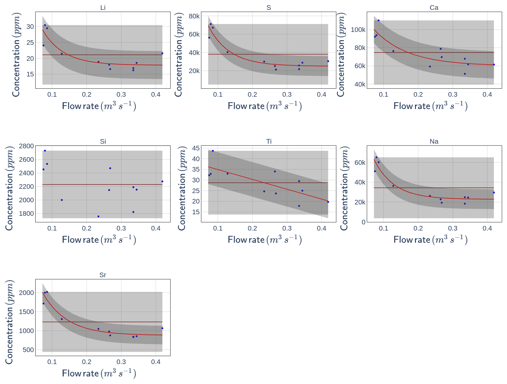
Figure A1 Relation between tracer concentration in the tributary “Arbres” and flow rate at the catchment outlet. Blue points are measurements, average concentrations are brown lines, and decreasing exponential functions are red lines (for relation with R² > 0.5). Uncertainties, defined as the maximum deviation between the fitted curve and the measurements are represented in grey: light grey for the average concentration function and dark grey for the exponential function.

Figure A2a shows that the methods MB_mean and MB_PCA,mean produce results that are very similar for EM_SR and slightly different for the sedimentary and quaternary contributions.

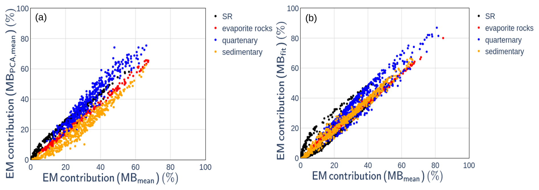
Figure A2 Comparison of end-member (EM) contributions obtained using different End Member Mixing Analysis methods: (a) MB_mean versus MB_PCA,mean; (b) MB_mean versus MB_fit.

Figure A2b shows that the adaptation of the end-member composition to the pre-event outlet flow rate has an impact on the decomposition results both for GW end members and EM_SR (particularly for contributions smaller than 0.3). We then need to determine which one of the two methods gives the most reliable results.

A2 Results of the EMMA decompositions on virtual mixings

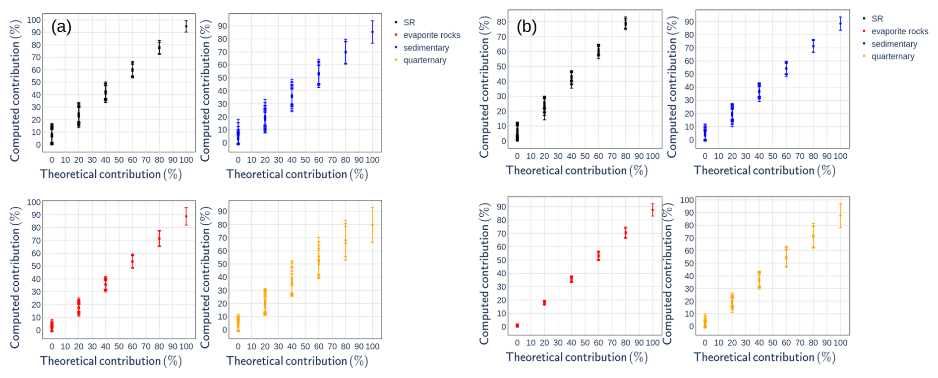
Figure A3 Results of the virtual test using the MB_PCA,mean (a) and MB_mean (b) End Member Mixing Analysis methods.

Virtual mixing were created with known contributions of the four end-members, as done in sediment fingerprinting studies (Batista et al., 2022). Figure A3 shows that both the MB_mean and MB_PCA,mean methods tend to slightly underestimate the contributions of all EM at high contribution rates, and tend to overestimate those of quartenary, sedimentary, and SR at low contribution rates. In this study, the focus was specifically on the accuracy of the models in predicting SR contributions within the range of approximately 0 % to 60 %. Within this range, Fig. A3 indicates that the MB_mean method performs best, even if this method tends to overestimate SR contributions by about 10 %. Overall, the virtual tests suggest that the MB_mean method seems to give better results than the MB_PCA,mean method. Comparison between MB_mean and MB_fit will be done in the next paragraphs.

A3 Results of the EMMA decompositions out of rainfall–runoff events

Figure A4 and Table A1 show that the methods MB_mean and MB_fit yield zero SR contributions up to a flow rate of approximately 100 L s⁻¹, which is a first good result. Beyond 500 L s⁻¹, both methods give considerable SR contribution (see Table A1), which is likely inaccurate and should be considered as an uncertainty assessment of the model, as these samples were selected outside of rainfall–runoff events. This suggests that the model uncertainty is below 5 % for hydrological state with flow rate inferior to 500 L s⁻¹, and around 10 % for hydrological state with higher flow rate (Table A1).

Table A1 also shows that for these presumed baseflow samples, the MB_fit model generally estimates slightly lower SR contributions than the MB_mean model.

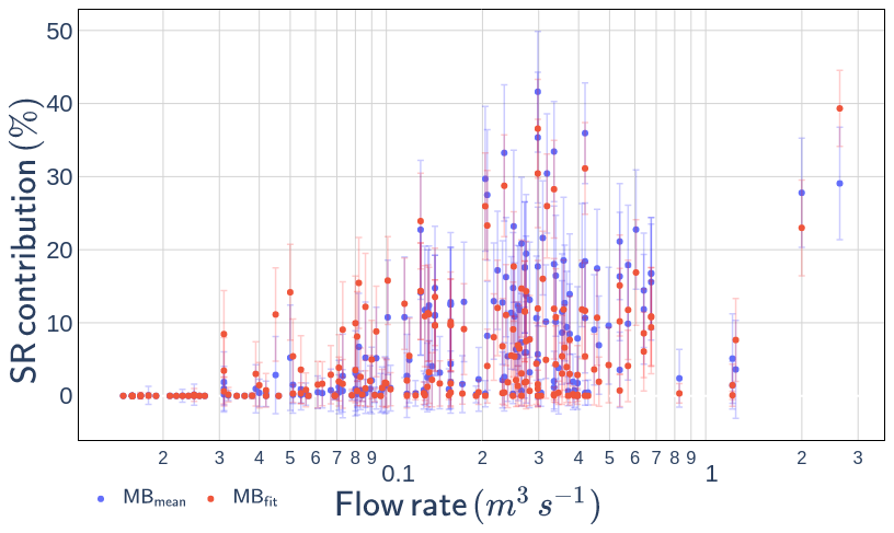
Figure A4 Surface runoff (SR) contribution for samples collected outside of rainfall–runoff events, calculated with the MB_mean and MB_fit End Member Mixing Analysis methods.

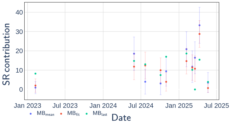
Figure A5 Surface runoff (SR) contributions for samples collected at the Galabre outlet during spatial campaigns, computed using the MB_mean and MB_fit methods, as well as the mass-balance approach based on the exact end-member compositions measured during the campaign (MB_last).

Table A1 Mean surface runoff contribution computed by the two End Member Mixing Analysis methods during periods out of rainfall–runoff events, for different flow rate ranges (Q, L s⁻¹).

Figure A5 compares the results obtained with the MB_mean and MB_fit methods, applied to samples collected at the catchment outlet during the spatial campaigns, with those derived from the MB_last method, which directly uses the chemical concentrations measured in each tributary during the last spatial campaign to define EM compositions. With the exception of two campaigns, the results produced by the MB_fit method are closer to those of the MB_last method than do the results from MB_mean. This provides additional support for adopting the MB_fit method.

A4 Results of the EMMA decompositions during rainfall–runoff events

Table A2 indicates that the MB_mean and MB_fit methods produce broadly comparable results during rainfall–runoff events, with average differences remaining below 3 % across all flow rate ranges. Table A2 shows that MB_fit generally estimates a slightly higher SR contribution at low flow rates and a lower SR contribution at high flow rates compared to MB_mean. As illustrated in Fig. A6, rainfall occurring under dry pre-event conditions tends to yield a higher SR contribution with the MB_fit model (up to +10 % on average) compared to the MB_mean model, whereas rainfall under wet pre-event conditions results in a lower SR contribution (up to −6 %). This behavior is consistent with the exponential adjustment applied in MB_fit: at low flow rates, the adjustment increases GW EM tracer concentrations, thereby enhancing the SR contribution in the mixing model. In contrast, at high flow rates, the adjustment reduces GW EM tracer concentrations, making them closer to river water chemistry and consequently lowering the estimated SR contribution in the mixing model.

Table A2 Mean surface runoff contribution and standard deviation computed by the two End Member Mixing Analysis methods during periods of rainfall–runoff events, for different flow rate ranges (Q, L s⁻¹).

Additionally, the use of regression models in the MB_fit method leads to reduced uncertainty in estimating SR contributions relative to the MB_mean model (Table A2). Based on these advantages, only the results from the MB_fit method are analyzed in the subsequent sections of this study.

The uncertainty of the SR contribution using the MB_fit method estimated by a Monte Carlo approach is approximately 6 % (Table A2). However, analyses of the model results, especially at low-flow conditions, suggest that the model is associated with additional intrinsic uncertainties due to its construction. Following these observations, the uncertainty on SR contribution is considered to be around 15 %.

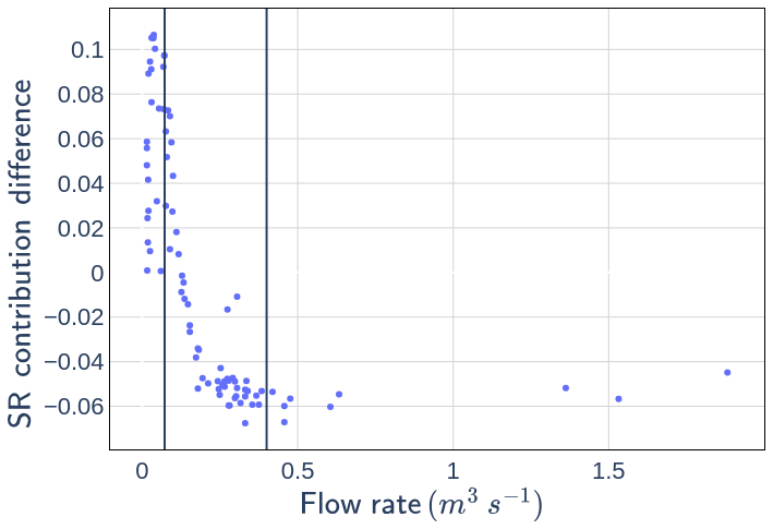
Figure A6 Event-averaged difference between the surface runoff (SR) contributions estimated by the MB_fit and MB_mean models, shown as a function of the initial flow rate of each event. The vertical lines indicate the flow-rate interval used to compute the adjustment between tracer concentration and flow rate (see Sect. 3.2).