the Creative Commons Attribution 4.0 License.
the Creative Commons Attribution 4.0 License.
 | 09 Oct 2018
Morphological effects of vegetation on the tidal–fluvial transition in Holocene estuaries
Ivar R. Lokhorst
Lisanne Braat
Jasper R. F. W. Leuven
Anne W. Baar
Mijke van Oorschot
Sanja Selaković
Vegetation enhances bank stability and sedimentation to such an extent that it can modify river patterns, but how these processes manifest themselves in full-scale estuarine settings is poorly understood. On the one hand, tidal flats accrete faster in the presence of vegetation, reducing the flood storage and ebb dominance over time. On the other hand flow-focusing effects of a tidal floodplain elevated by mud and vegetation could lead to channel concentration and incision. Here we study isolated and combined effects of mud and tidal marsh vegetation on estuary dimensions. A 2-D hydromorphodynamic estuary model was developed, which was coupled to a vegetation model and used to simulate 100 years of morphological development. Vegetation settlement, growth and mortality were determined by the hydromorphodynamics. Eco-engineering effects of vegetation on the physical system are here limited to hydraulic resistance, which affects erosion and sedimentation pattern through the flow field. We investigated how vegetation, combined with mud, affects the average elevation of tidal flats and controls the system-scale planform. Modelling with vegetation only results in a pattern with the largest vegetation extent in the mixed-energy zone of the estuary, which is generally shallower. Here vegetation can cover more than 50 % of the estuary width while it remains below 10 %–20 % in the outer, tide-dominated zone. This modelled distribution of vegetation along the estuary shows general agreement with trends in natural estuaries observed by aerial image analysis. Without mud, the modelled vegetation has a limited effect on morphology, again peaking in the mixed-energy zone. Numerical modelling with mud only shows that the presence of mud leads to stabilisation and accretion of the intertidal area and a slight infill of the mixed-energy zone. Combined modelling of mud and vegetation leads to mutual enhancement with mud causing new colonisation areas and vegetation stabilising the mud. This occurs in particular in a zone previously described as the bedload convergence zone. While vegetation focusses the flow into the channels such that mud sedimentation in intertidal side channels is prevented on a timescale of decades, the filling of intertidal area and the resulting reduction in tidal prism may cause the infilling of estuaries over centuries.
- Article
(15060 KB) - Full-text XML
- BibTeX
- EndNote


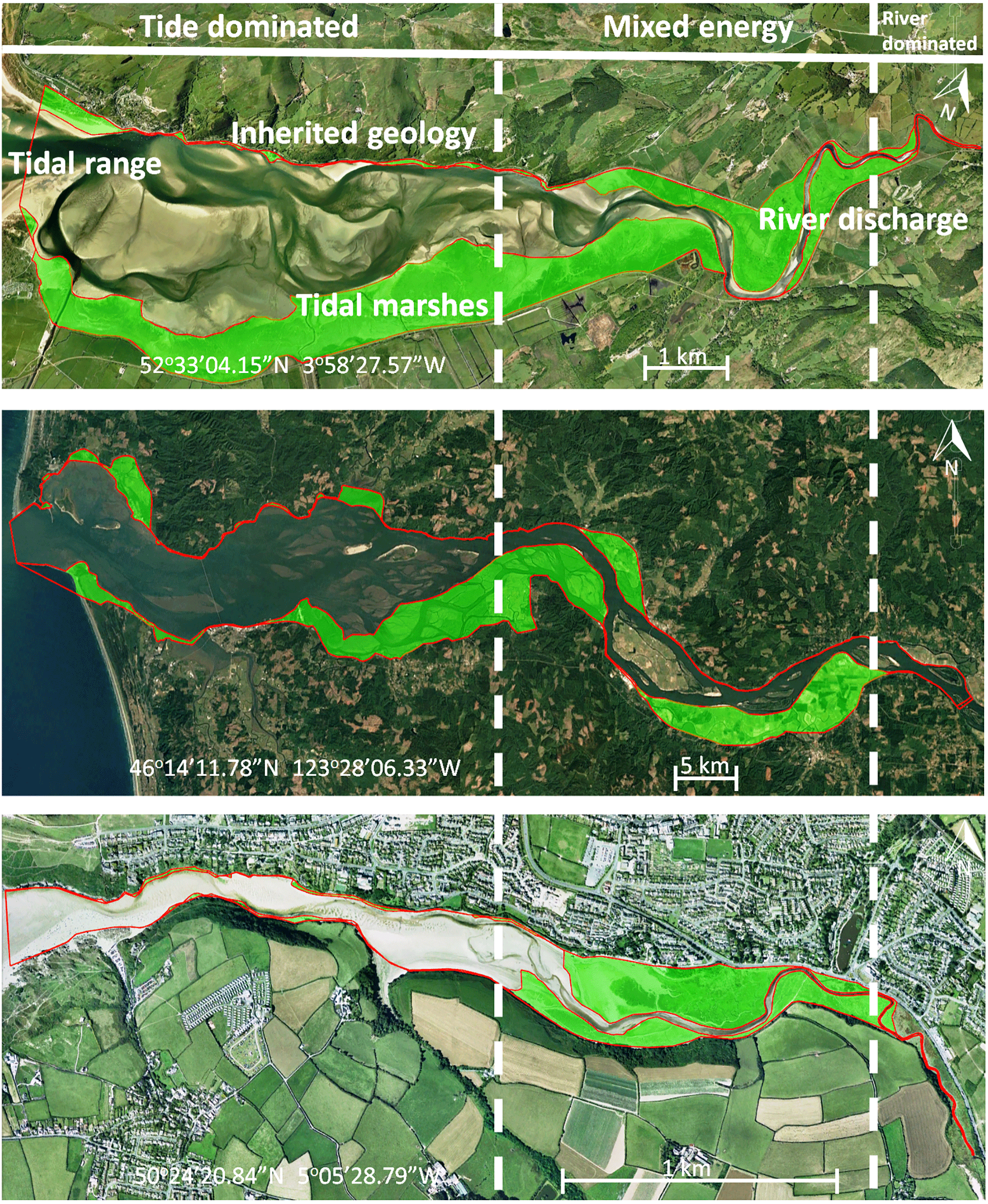
Figure 1Active and vegetated parts of estuaries, showing proportionally more vegetated area in the upstream transition from single-thread river to multi-thread estuary. The estuaries are the Dyfi (UK), Columbia (USA) and Gannel (UK). The green areas are the vegetated parts of the estuary while the red lines project the morphologically active areas. Distinctions between dominant energy types are based on characteristic morphological features like tidal creeks, intertidal area, irregular shaped tidal bars and large meanders (Dalrymple et al., 1992).
1.1 Problem definition
Estuaries are flanked by tidal marshes, which are unique ecosystems with a very high biomass that modify the local hydromorphodynamic conditions (Davidson et al., 1991; Friedrichs, 2010; Meire et al., 2005). Vegetation affects hydromorphodynamics in rivers (Corenblit et al., 2009; Oorschot et al., 2015), and this effect on hydromorphodynamics has also been shown on the scale of individual tidal marshes (Bouma et al., 2005; D'Alpaos et al., 2006; Temmerman et al., 2007). The effect of vegetation on hydromorphodynamics in tidal marshes is therefore relatively well known on the individual plant or patch scale (Järvelä, 2002; Siniscalchi et al., 2012), while its effect on estuary-scale morphodynamics has barely been studied. Incorporating vegetation in estuarine morphodynamic models is considered one of the three biggest challenges to overcome in modelling the long-term evolution of tidal networks (Coco et al., 2013). A comprehensive but qualitative model suggests that tidal marshes reach their largest extent in the mixed-energy zone of the estuary (Dalrymple et al., 1992). Here we investigate whether plant species can collectively have eco-engineering effects that are significant enough to modify entire estuarine landscapes. As we do not differentiate between different types of marshes, we will use a generic marsh species which will be referred to as either tidal marsh or marsh.
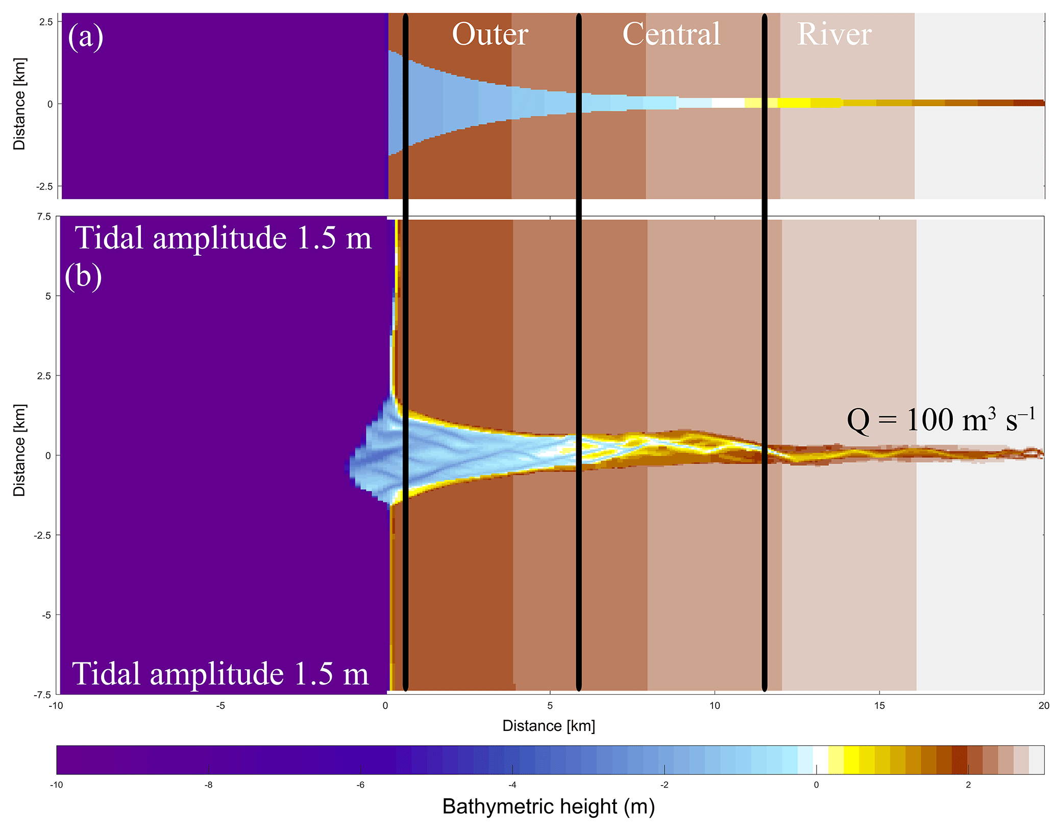
Figure 2Initial model conditions. (a) The original initial bathymetry in Braat et al. (2017). (b) The bathymetry after 1000 years of simulation (Braat et al., 2017), which is the initial bathymetry for the present model runs. Bold lines indicate division between the outer, middle and river part of the estuary based on the decrease in flood velocity along the estuary.
In rivers, riparian vegetation stabilises channels by reducing floodplain flow and adding bank strength to the floodplains (Corenblit et al., 2009; Gurnell et al., 2012). These eco-engineering effects can be strong enough to cause the transition from braiding towards meandering or even sinuous rivers (Dijk et al., 2013; Ferguson, 1987; Oorschot et al., 2015; Tal and Paola, 2007). However, the presence of vegetation can also cause the bifurcation of channels by stabilising bar tips, causing flow resistance on point bars and diverging the flow from the channel onto the floodplain (Burge, 2005; Dijk et al., 2013). Furthermore this increased flow resistance causes flow to decelerate and water levels to rise, which may induce flooding events (Darby, 1999; Kleinhans et al., 2018). The presence of mud has a partly similar effect to vegetation because it can lead to the stabilisation of systems as well, and mud has shown to preferentially accumulate in vegetated areas (Kleinhans et al., 2018). Based on these insights and general similarities between rivers and the tidal–fluvial transition, it is easily conceivable that similar biogeomorphological interactions shape upstream parts of estuaries. While salinity is an important variable determining which species prevail, here we focus on a single and often dominant tidal marsh vegetation species.
Tidal marsh vegetation flanks estuaries from the brackish zone to the mouth. Tidal marsh enhances sedimentation both through reduced flow velocities and through particle capture, somewhat comparable to what happens on river floodplains, but tidal marsh is not considered a particularly effective channel and bank stabiliser (Allen, 1994; Bouma et al., 2007; D'Alpaos et al., 2006; French, 1993; Lee and Partridge, 1983; Mudd et al., 2010). If the hydroperiod, the time that tidal marshes are submerged every day, gets longer the sediment supply to the marsh increases and therefore so does the sediment accretion. Several authors therefore found that tidal marshes are most productive at a certain rate of sea level rise (SLR) because this keeps the hydroperiod more or less constant as accretion rates balance with SLR (Orson et al., 1985; Redfield, 1972). However, tidal marshes may drown when the sea level rise rate is too large relative to the sediment supply, which leads to vegetation loss and therefore marsh drowning at an enhanced rate (Kirwan and Temmerman, 2009). In general, tidal marshes are thought to approach an equilibrium level relative to the sea level whether rising or not (Friedrichs and Perry, 2001; Marani et al., 2013).
For tidal marsh to accrete, the supply of mud is essential as the source of inorganic accumulation. This mud may have a coastal or fluvial source, and the main source might have significant effects on the evolution of the estuary (de Haas et al., 2017). Although mud is transported in suspension and thus reaches higher, low-energetic elevations and areas more distal from the main channel, it is not unlimited. Suspended sediment rapidly settles in tidal marshes and therefore the concentration in the water quickly decreases with distance into the marsh (Townend et al., 2011). Nevertheless, cohesive mud is more difficult to erode than sand when it consolidates, so that on the estuary-scale mud leads to narrower systems with reduced bar dynamics through mudflat accumulation (Braat et al., 2017). The logical hypothesis is that the added effect of vegetation leads to even more accretion at the flanks of the estuary (Brew and Williams, 2010).
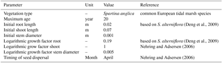
Braat et al. (2017)Braat et al. (2017)Braat et al. (2017) (Deng et al., 2009)(Deng et al., 2009)Nehring and Adsersen (2006)Nehring and Adsersen (2006)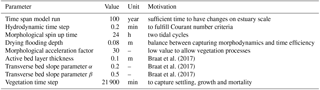
Table 2Parameterisation of general characteristics of Spartina anglica.
The availability of mud is partly determined by the changing hydrodynamic energy along the river continuum, especially in shallow, well-mixed estuaries that we focus on (Fig. 1) (Dalrymple et al., 1992). The tidal–fluvial transition appears to be a zone of sand and mud convergence, both of which are therefore conducive to tidal marsh establishment (Fig. 1). Alternatively, it could be the mixed-energy setting that is conducive to tidal marsh establishment, which, in turn, enhances sedimentation. A central zone of lower energy where the average grain size decreases has been observed where bedload converges (Johnson et al., 1982). Bedload convergence means that both the river and the sea transport more sediment towards this central zone in the estuary than they export, resulting in net accumulation. Dalrymple et al. (1992) suggested that this area of bedload convergence often coincides with the relatively largest tidal marsh extent (Fig. 1). Furthermore, in many estuaries a turbidity maximum zone (TMZ) occurs in the same mixed-energy zone of the estuary, which are characterised by elevated suspended sediment concentrations (Brenon and Le Hir, 1999). It is important to realise that the relative contribution of the tides, river and waves to the total hydrodynamic energy is gradually changing along the estuary (Dalrymple et al., 1992). We will use a rough classification of the estuary into an outer, central and river part, which is characterised by a dominance of tides, mixed importance of tides and river, and dominance of the river over hydrodynamics respectively.
Our hypothesis derives from a combination of three independent and complementary analyses. First, a reconstruction of the Holocene development of estuaries and tidal basins suggests that vegetation combined with mud tends to infilling of estuaries. Through a reduction in intertidal water storage at the system margins, due to vegetation-enhanced sedimentation, the tidal prism reduces and tends towards flood-dominant transport (Friedrichs, 2010; Friedrichs and Perry, 2001; Speer and Aubrey, 1985). Second, a large number of estuaries fill all space wider than that covered by an idealised convergent estuary with tidal bars (Leuven et al., 2017). This analysis excluded tidal marshes, but clearly a number of estuaries were larger in the past and have at least partly been filled by mudflats, tidal marsh or mangroves. A model study by Braat et al. (2017) on the effects of mud on the system-scale development of estuaries over millennia showed that mud decreases the morphodynamics and decreases the total system width depending on mud concentration. All three approaches – geological, remote sensing and numerical – point to system-scale effects of mud and vegetation in estuaries.
Our aims are to determine the combined effects of mud and vegetation on estuarine planform and morphodynamics, specifically in the setting of a sandy estuary with mud input from the river. To this end we will use a numerical model for a century-scale simulation of flow, sediment transport, morphology and vegetation. We ignore the binding of sediment by roots because of the relatively shallow rooting and only explore the cohesive effects of mud, the floodplain-filling effects of mud and the flow resistance effects of vegetation. This allows us to apply an existing model for riparian vegetation to the tidal environment. Two questions of specific interest are how the zonation of vegetation, as found by Dalrymple et al. (1992), can be explained and what the morphological and hypsometric changes are as a result of the presence of vegetation.
Nehring and Adsersen (2006)Table 3Parameterisation of life-stage-specific characteristics of Spartina anglica.
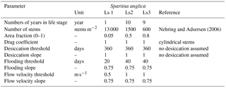
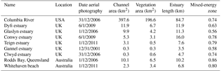
Table 4Channel area, vegetation area and estuary length derived from polygons digitised in Google Earth, accessed October 2017. The mixed-energy zone gives the approximate distance of the mixed-energy zone as a fraction of the distance from the estuary mouth.
To investigate whether the transition of dominantly fluvial energy to dominantly tidal energy is indeed the hotspot of sedimentation and tidal marsh formation, we combine a vegetation model with the morphological estuary model built in Delft3D by Braat et al. (2017), which includes cohesive sediment. Tidal marsh modelling is based on the recently developed riparian vegetation model by Oorschot et al. (2015). This model takes the vegetation cycle into account, which includes colonisation, growth and mortality due to flooding, uprooting, scour and high flow velocity. The processes of settlement, growth and mortality are similar for riparian and tidal marsh vegetation and the process of flow retardation due to flow obstruction remains a function of stem height, width and density. So, with a different parameterisation for plant growth, dimensions and mortality, we were able to realistically represent marsh vegetation with this model. We modelled the combined effects of mud and vegetation to investigate feedback mechanisms between these two and compare the model results with measurements in nine real estuaries.
The model consists of two interacting codes: the hydromorphological modelling package Delft3D version 4.01.00 and our MATLAB-based vegetation module. The coupling is fast and the vegetation module slows down the model marginally, mainly due to file input and output. However, the need to compute at a very high temporal resolution leads to model runtimes for up to 2 months to simulate 100 years of development. To investigate the combined effects of mud and vegetation, an existing model schematisation was used that is loosely based on the Dyfi estuary in Wales (Braat et al., 2017). The large computation times of the interacting codes necessitated that our model start from the well-developed morphology after 1000 years. To isolate the effect of vegetation in the simplest possible settings, we ignore salinity, waves and tidal components other than M2. The tidal marsh vegetation is represented by the settling, growth and mortality traits of Spartina anglica and the hydraulic resistance as a function of stem dimensions and density as detailed later. Although Spartina anglica is not the only pioneer species in these systems (e.g. Salicornia), the vegetation modelling here is simplified, given the large spatiotemporal scales and first application of a vegetation model. In our runs, the vegetation traits based on the commonly occurring Spartina anglica are to be seen as a generic tidal marsh plant species.
2.1 Hydromorphodynamic model
Delft3D is a widely tested open-source model that can calculate both sand and mud transport. The 2DH (depth-averaged) version was used with a parameterisation for bend flow effects on the direction of sediment transport. We used a rectangular grid, which affects the form of the equations given below. Here we will state the main equations used in Delft3D, which are either default or activated by choice. The only equations incorporated into our MATLAB model are related to the settling, growth, mortality and bookkeeping of the vegetation.
The model is mainly based on two hydrodynamic equations, the first being the conservation of mass equation:
where h is the water depth, t is time, u is the flow velocity in the x direction and v is the flow velocity in the y direction. Equation (1) states that any change in water depth follows from a discharge gradient in the x direction (qx) or a discharge gradient in the y direction (qy) for a 2-D model. Momentum conservation is calculated as
where zw is the water surface height, C is the Chézy roughness, which will be calculated by the vegetation model described below, V is the horizontal eddy viscosity and Fx,y is the streamline curvature-driven acceleration term (Schuurman et al., 2013). These two equations describe the velocity variations in the x–y plane in one grid cell over time under the influence of advection, eddy diffusivity, friction, changing water depth and streamline curvature. Sediment transport is calculated by separate equations for the different sediment constituents. Sand transport in the case of a non-cohesive bed is calculated with the Engelund–Hansen sediment transport predictor:
where ρs the sediment density, ρw the water density and D50 the median grain size. The sediment transport of the mud fraction of the model is calculated by Partheniades–Krone equations (Partheniades, 1965) for erosion flux Em,
and for deposition flux Dm:
for , where τcw is the maximum bed shear stress due to currents, τcr,e is the critical erosion shear stress, Mm is an erosion parameter, ws is the mud settling velocity and cb the average sediment concentration in the near-bottom layer. Above a critical mud content threshold (), the sand and mud flux are proportional to their respective fractions in the sediment bed. Mud erosion is the same in the cohesive and non-cohesive regime, but the sand erosion becomes dependent on the mud entrainment in the cohesive regime, when the mud content in the bed exceeds 40 %. The transport of sand becomes fully dependent on the mud flux, as bedload transport is assumed to be zero in the cohesive regime. Once sediment is suspended following the Partheniades–Krone equation, it is transported by the advection–diffusion equations. A constant mud settling velocity of m s−1 was assumed based on Braat et al. (2017).
A parameterisation is needed for helical flow due to streamline curvature in a depth-averaged simulation to create point bars in river bends and estuarine bars and is included as follows. The bedload transport direction ϕτ is given by the following equation:
where U is the depth-averaged flow velocity, Is is the spiral flow intensity factor, here taken at unity, and αI is given by the following equation:
where κ is the von Kármán constant, taken as 0.41. Lastly, bed slope effects are included in the model to simulate a deviation in sediment transport direction from the shear stress direction due to grains moving downslope. The sediment transport in the x and y direction under influence of the bed slope effect is given by
where qs is sediment transport, zb is the bed height, and f(θ) is given by the following equation:
In this equation θ is the shields parameter and α and β are calibration parameters specified later.
2.2 Vegetation model
A model programmed in MATLAB was used to simulate the vegetation in the estuary (Oorschot et al., 2015). This model simulates vegetation colonisation, growth and mortality and translates this to hydraulic roughness used in Delft3D as based on the Baptist et al. (2007) equation:
where C is the Chézy roughness value due to the bed and vegetation roughness (), Cb is the Chézy value for the bed without vegetation, Cd is the drag coefficient, n is the number of stems per square metre times the stem diameter, hv the vegetation height and κ=0.41 is the von Kármán constant. Vegetation of different ages and therefore with different characteristics can occur simultaneously in one grid cell up to a total fraction of 1. The Chézy value is calculated for each age class, and afterwards a total Chézy coefficient is calculated based on the fraction coverage of each age class.
The vegetation model divides the morphological year into 24 ecological time steps, which correspond with half a month of morphological development (Table 1). Following each ecological time step the hydromorphodynamic calculations are stopped and the bed level changes, water levels and flow velocities are exported from Delft3D to the vegetation model. A 2-week interval, during which vegetation properties are assumed constant, was chosen to capture the dominant vegetation development processes. Over a 2-week growth period, the species have no appreciable changes in size, and this time step balances with the computational cost that increases with a decreasing time step. The vegetation has both general and life-stage-specific characteristics (Tables 2 and 3). General characteristics are the seedling dimensions, i.e. shoot length and diameter and root length, maximum age, growth factors for logarithmic shoot, root and diameter development, and seed dispersal timing (Oorschot et al., 2015). Life-stage-specific characteristics are rules for mortality due to flooding and uprooting, number of stems per area, drag coefficient, and fraction of the grid cell surface covered with vegetation. All the variables in the Baptist et al. (2007) equation are thus accounted for. The new vegetation characteristics are then used to update the Chézy roughness field in Delft3D.
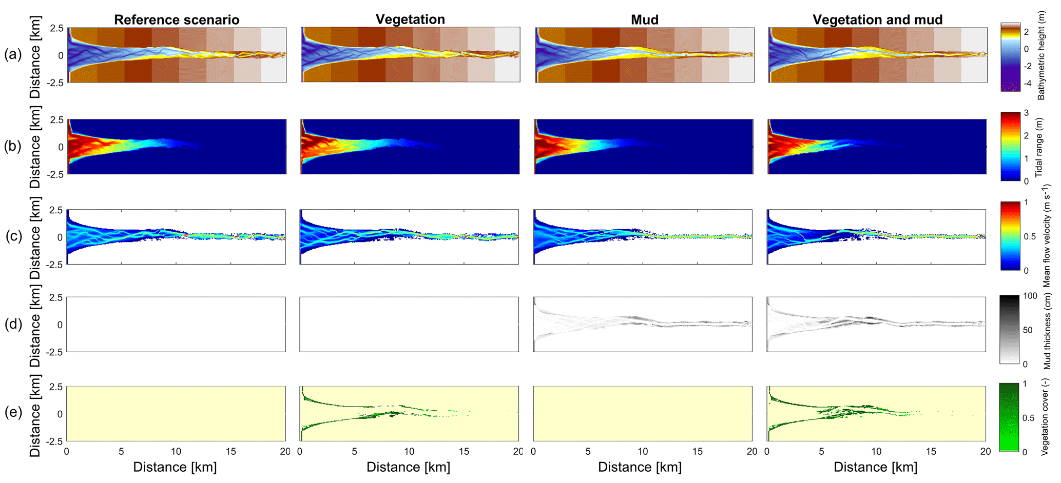
Figure 3Results of the four scenarios after 100 years of simulation. (a) Morphology. Colours representing larger depths than −5 m were saturated to enhance contrast. (b) Tidal range. (c) Mean of absolute flow velocity during the tidal cycle. (d) Mud thickness in cm. (e) Vegetation cover at the surface, ranging from 0 to 1.
Colonisation takes place during the month of seed dispersal on every location where water has been present (Table 2). This means that all cells in the intertidal zone are colonised with Spartina anglica by the predefined colonisation density. Given that the tides in the model are simplified to M2, the supratidal zone where vegetation settles in nature can be seen as included as high intertidal. There is no seed dispersal module other than that we assume the seeds to spread through the water (hydrochorously), and neither do seeds end up above the water surface. This means that seedlings colonise lower intertidal areas, after which mortality determines which plants survive such that the lower intertidal zone is not occupied by plants during the flow modelling. We do not model rhizomic growth since this is a process occurring at a much smaller spatial scale than the grid cell size.
The vegetation follows a logarithmic growth function dependent on age, which limits their growth once they mature:
in which G is the length or diameter of the shoot or root, Fv is a characteristic growth factor for the root or shoot, and a is the vegetation age in years. The initial dimensions of the seedlings are defined in the general characteristics, after which plant growth is calculated yearly following the equation.
Mortality is calculated yearly as a function of burial, uprooting, maximum flow velocities, flooding and ageing. Burial and uprooting are determined by comparison of the plant dimensions and bed level change. If the erosion in an ecological time step exceeds the length of the root, the plant is uprooted, and if the sedimentation exceeds the shoot length, it is considered buried, both leading to mortality (Oorschot et al., 2015). To calculate mortality due to flooding and flow velocity, the maximum, minimum and average water depth at each cell are determined during the tidal cycle. Because tidal marsh vegetation starts to occur above mean tide and usually quickly accretes to the high tide mark, the subsequent days that the cells are flooded during mean tide are recorded. For flow velocity, the maximum value during the tidal cycle in each cell is stored. Lastly, vegetation dies when its maximum age is reached.
A dose–effect relation (Oorschot et al., 2015) is applied to model gradual plant demise as the fraction of plants that do not survive the hydrodynamic pressure. Until a threshold is exceeded no mortality occurs, while above this threshold an increasing portion of the plants start dying with increasing stress. The threshold value and the slope of the stress–mortality relation are user-defined and can vary between the life stages of the plants (Table 3). Mortality was applied to each age class in all grid cells (Oorschot et al., 2015).
2.3 Model set-up
We set up four model scenarios based on our earlier work and about 30 preliminary test runs, where we balanced time efficiency and the processes that could be realistically represented (Braat et al., 2017; Oorschot et al., 2015).
The initial bathymetry is the final outcome of a model run that started from an idealised convergent shape (Braat et al., 2017). This avoids long computational time to develop sufficient bars and mudflats where vegetation can settle. The rectangular cell size varies from 50 m by 80 m in the estuary to 125 m by 230 m offshore. This is done to balance computational time and sufficient spatial resolution. A 0.2 min time step was used based on the Courant criterion. We applied a 1.5 m tidal amplitude defined by two harmonic water levels at the north and south coastal boundaries and a constant 100 m−3 s−1 discharge at the upstream river boundary. The bed is initially entirely composed of sand and has a sand supply equal to the transport capacity at the river boundary, which avoids sedimentation or erosion at the upstream boundary. Mud, on the other hand, is supplied as a constant concentration at the upstream boundary of 20 mg L−1, the same as in the run by Braat et al. (2017) that led to large-scale equilibrium of the estuary planform. This model was run for 1000 years without vegetation in Braat et al. (2017), and the final bathymetry was used as the initial condition for further simulations including vegetation (Fig. 2b). Note that this bathymetry was the result of calculations including mud. However, we only use the initial bathymetry and not the bed composition as our initial condition in order to isolate the effect of the addition of vegetation and mud through the upstream supply.
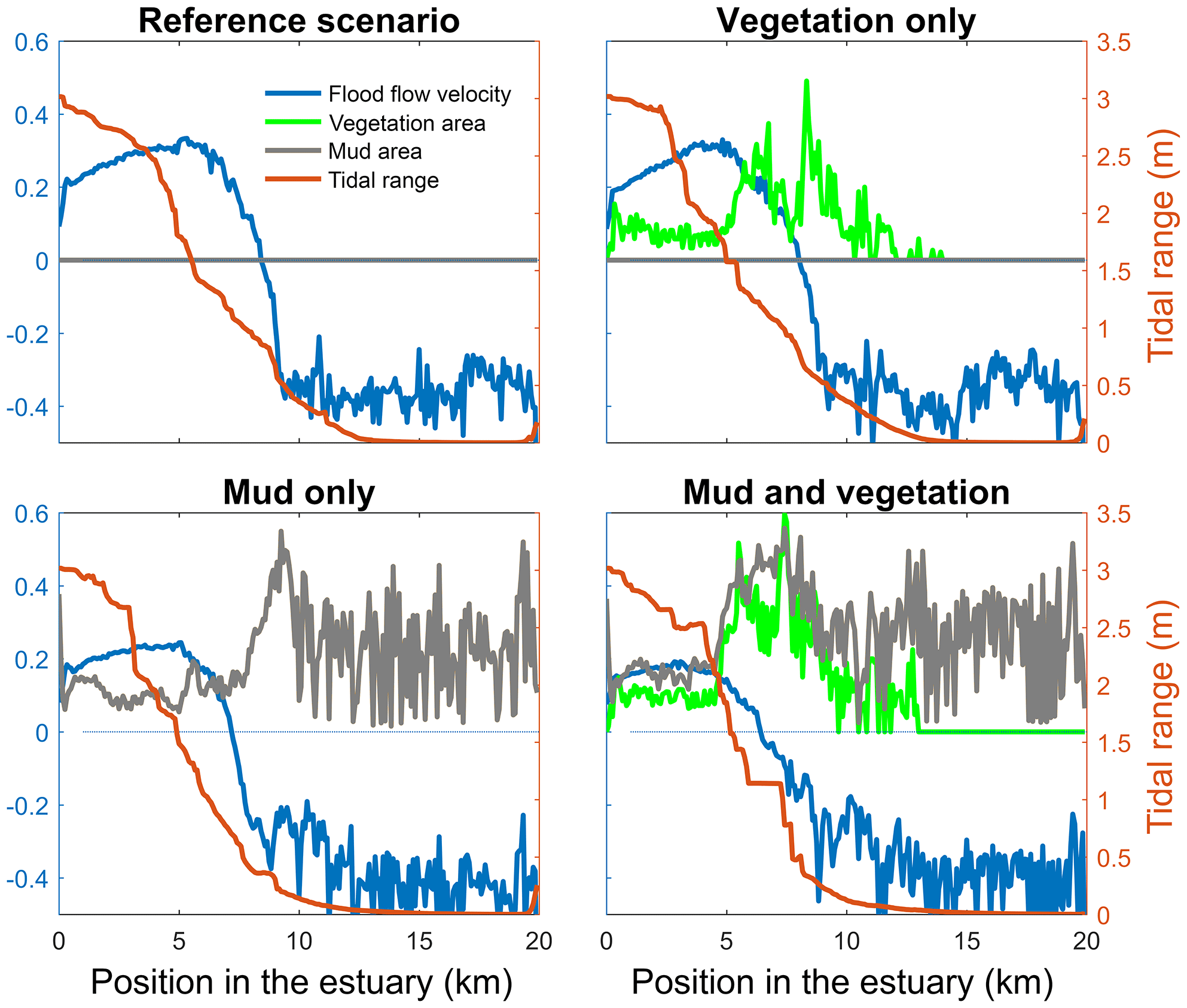
Figure 4Tidal range, maximum flood flow velocity, vegetation cover and mud cover as a fraction of the estuary width plotted against landward distance from the coastline. In all four figures the left axis is used for three variables: width averaged flood velocity, mud cover and vegetation cover. The right axis is used for the maximum tidal range of the estuary cross section in all four subplots.
2.4 Parameters and scenarios
Several parameters for hydromorphodynamic processes, numerical processes and vegetation development were varied (Table 1) to study their effect on estuary developments. Model scenarios were run for 100 years, which is about the minimum time required for morphological changes at the system scale to occur due to vegetation and the practical maximum time given computational and input–output costs of about 2 months on a single node in a fast desktop computer (Table 1). A small morphological scale factor of 30 was used, since preliminary testing showed that this allowed vegetation settlement, growth and mortality over a number of tidal cycles without significant morphological change. In contrast, for sandy estuaries without vegetation, values up to 1000 have been used (Van der Wegen and Roelvink, 2008). In the vegetation model a balance is required between morphological and hydrological timescales, since these both affect the development of the plants. If the morphology changes significantly faster than the hydrodynamics, plants are subject to large-scale burial and uprooting. A default Chézy value of 50 for bare sediment was chosen as in Braat et al. (2017). Vegetation traits of Spartina anglica were based on Nehring and Adsersen (2006) and Deng et al. (2009) (Tables 2, 3).
2.5 Data collection of real estuaries
For a first quantitative comparison of model results with real estuaries, we mapped along-channel variability of unvegetated channel width and width of the vegetated zone in nine natural estuaries. The real estuaries were selected from the dataset of Leuven et al. (2017) based on the presence of tidal marsh vegetation and include one system with mangrove species (Table 4).
The area of each estuary was visually classified as either unvegetated or vegetated in Google Earth. The unvegetated polygons come from the dataset by Leuven et al. (2017), and this analysis adds polygons of the vegetated area (Fig. 1). The vegetated area comprises the area that borders the active estuary and is covered with pioneering or fully grown tidal marsh vegetation. The presence of sinuous tidal creeks and vegetation other than, for instance, forest, were used as an indicator of present-day or recent tidal influence and older riparian vegetation was excluded. Tidal vegetation was distinguished by its different colour compared to surrounding forests and grass fields and by its clumpy and patchy structure. The elevation data in Google Earth were used as further evidence for the outer boundary of the tidal vegetation area to avoid steep gradients and cliffs at the transition from a supratidal elevation level to higher elevated areas bordering the estuary.
Subsequently, centre lines of the polygons were constructed along the channel, which allowed width measurements perpendicular to this centre line (Leuven et al., 2017). This resulted in along-channel profiles of the active channel width, summed width of vegetation and estuary width, in which the estuary width is defined as the active channel width including bars plus the summed width of vegetation. The along-channel distance from the mouth was normalised with the length of the estuary. Estuary length is defined as the length from the mouth up to the point where the estuary width is equal within a few percent to the active channel width, in our case the upstream river. By this normalisation a direct comparison is possible between estuaries with different lengths and our modelled simulations. Through this normalisation it becomes possible to compare estuaries with different tidal–fluvial dominance. Estuaries with a small river might have a smaller, more upstream, mixed-energy zone than estuaries with a larger river. As the mixed-energy zone is a somewhat objective designation because it is part of a continuum, we investigate vegetation cover as a function of the normalised position in the estuary and as a function of total energy. By doing this we do not delimit the mixed-energy zone but compare vegetation cover development with the development of the total energy along the estuary.
Estimates of local tidal prism and total energy were made for each of the real estuaries based on Leuven et al. (2017). Local tidal prism was estimated by multiplying the along-channel width profile with the tidal range profile and integrating over the distance upstream of a given point. The volume added by the river was characterised by river discharge multiplied by tidal period. We then calculated a characteristic velocity by dividing the local prism TP by the local active width Wa and half the tidal M2 period TM2∕2. As a proxy for the total flow energy, this velocity was taken to the power of 3 as this is also a common indicator of sediment movement (Aubrey and Speer, 1985), so that flow energy is here calculated as 2TP(WaTM2)−3.
3.1 Effects of mud and vegetation on the entire estuary
The mouth of the modelled estuary has a 3 m tidal range, which decreases gradually in the landward direction to disappear roughly 14 km into the estuary (Fig. 3). The flow velocity, on the other hand, increases in the outer part of the estuary because the convergence is stronger than the friction. Further in the estuary the convergence decreases and the increase in friction begins to dominate, which results in a decreasing flood velocity. Therefore, there is a peak in the flood flow velocity at roughly 5 km into the estuary (Fig. 4). The changes in tidal range along the estuary are thus similar to those in a hyposynchronous system while the changes in the current are similar to those in a hypersynchronous system (Fig. 4).
In the simulation without mud and vegetation, i.e. the reference scenario, channels and shoals are dynamic, but no system-scale changes occur as the initial system seems to be close to dynamic equilibrium. Only a slight change in hypsometry occurs: the intermediate heights are slightly eroded, while the higher parts accrete slightly (Fig. 5).
The simulation with vegetation only develops fringing marshes at the edges of the estuary. The marshes start from the estuary mouth up to the tidal limit, roughly 14 km upstream (Fig. 3). The relative width of the tidal marshes is fairly constant at ≈10 % of the estuary width in the outer zone. Between roughly 6 and 11 km, however, the relative width of the marshes suddenly increases. The relative width of the tidal marshes can go up to 60 % of the estuary width. This area coincides with the area where the flood velocity and river velocity start to decrease due to friction and estuary shape respectively (Fig. 4). Beyond 14 km there is no vegetation anymore; this is because this is beyond the tidal limit and therefore there is no drying and flooding area where seeds are distributed and seedlings survive. The morphology in the simulation with vegetation only shows little differences compared to the reference simulation. This indicates that the vegetation is unable to enhance sedimentation in the absence of suspended fine sediment and that it predominantly colonises locations that are not prone to erosion because there is no significant reduction in the erosion of the intertidal area (Fig. 5).
The simulation with mud only results in a fairly continuous mud cover along the entire estuary (Fig. 3). There are small amounts of mud which deposit on tidal bars, in the order of an accumulated 10 cm admixed in sand over 100 years, but the more pronounced accumulations occur on the edges of the system. Similar to the simulation with vegetation the relative mud abundance starts to increase landward of the maximum flood velocity, which occurs at roughly 6 km. The relatively large mud extent in the central zone of the estuary is due to the low flow velocities in this zone (Figs. 3, 4). Unlike the vegetation cover, however, the relative mud abundance does not decrease to zero at the tidal limit, but approaches a roughly constant value of approximately 30 % of the system width (Fig. 4). This is because the estuary is small in this area, as the river is only several cells wide, and not because there are large extensive mudflats. In terms of hypsometry the largest effect of mud is that the intermediate bed elevations increase slightly (Fig. 5). This shows that the higher elevations are nearly filled as much as possible, and that the estuary develops in a feedback of further filling and reduction in tidal prism.
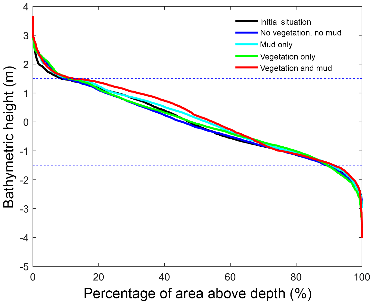
Figure 5Hypsometry of the entire estuary after 100 years. Dashed lines indicate the tidal range at the seaward boundary. Around 70 % of the estuary area is intertidal in all scenarios, indicating that the model represents a shallow system. The hypsometry is determined over the surface occupied by the estuary of the initial condition, which excludes new areas formed by bank erosion that is modelled rather simplistically in Delft3D.
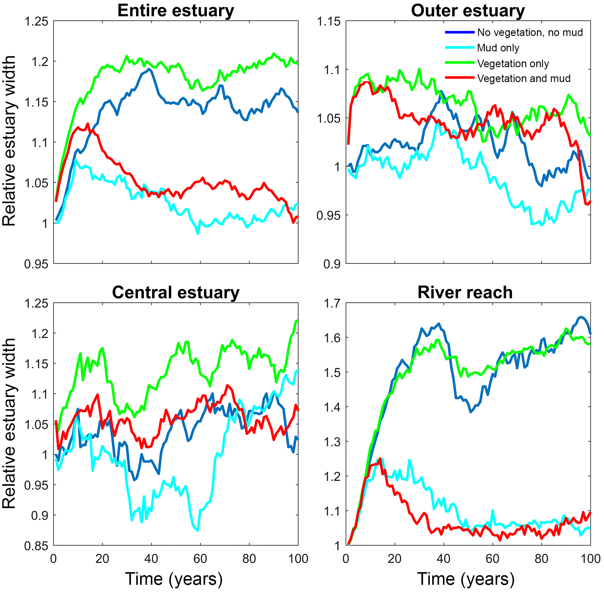
Figure 6Estuary width over time for of the entire system and for zones along the estuary. Width is normalised by average initial width. See Fig. 2 for locations of zones.
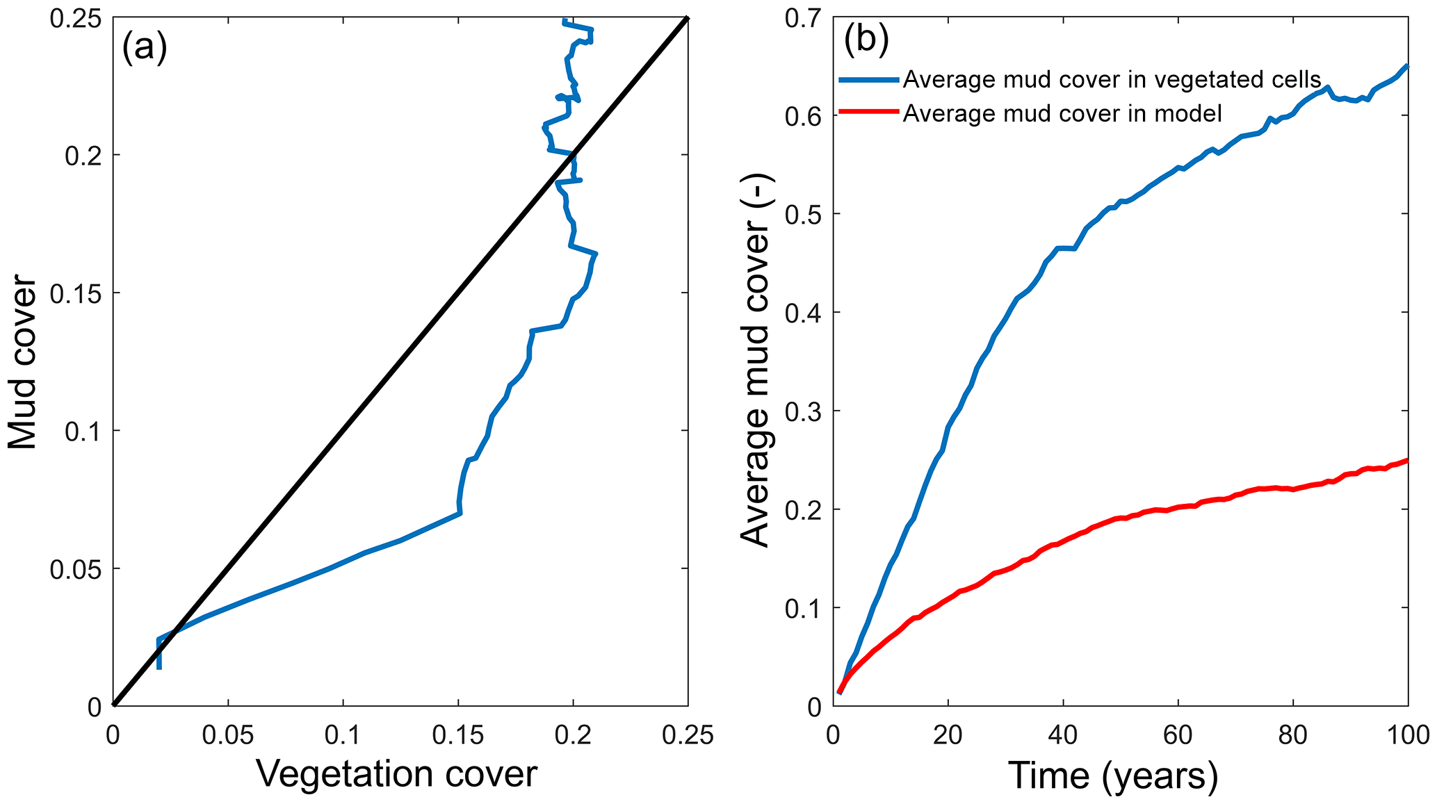
Figure 7Interaction of mud and vegetation. (a) The development of the total mud and vegetation cover over time in the simulation where both are present, where the simulation begins in the origin of the plot. Black line indicates equality of mud and vegetation cover. (b) The average mud cover in vegetated cells and in the entire model, showing substantially higher cover in vegetated cells.
The distribution of vegetation and mud in the combined simulation shows similar patterns to the simulations with either mud or vegetation only. There are some marshes and mud deposits in the outer estuary, but these become more pronounced towards the central zone (Fig. 3). There is a positive feedback between mud and vegetation. Not only do mud and vegetation occur in the same area, but their relative abundance also increases compared to simulations where one of them is absent (Figs. 3, 4). This is emphasised by the total mud and vegetation cover in the estuary, which are almost identical after 100 years (Fig. 7a). There is an especially strong feedback in the beginning of the simulation, when vegetation cover increases strongly, after which mud cover starts to increase faster (Fig. 7a). On top of that, the addition of vegetation to the simulation with mud further enhances the aggradation of the upper hypsometric heights and thus the intertidal area.
3.2 Effects of mud and vegetation in the mixed-energy zone
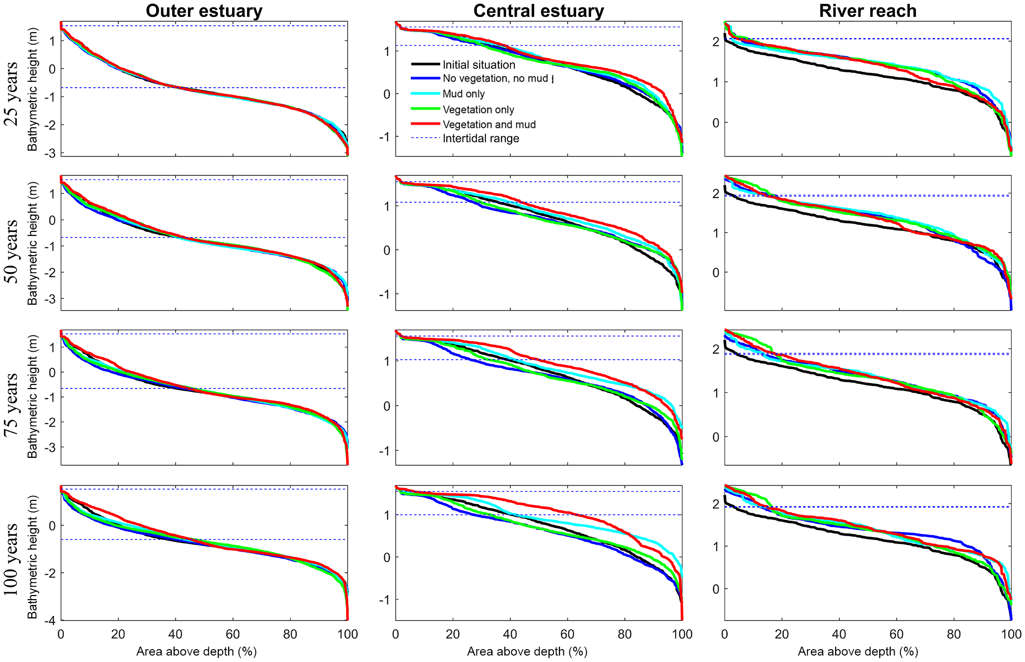
Figure 8Development of hypsometry of three zones in the modelled estuaries. The outer estuary has a concave shape while the central and river areas have a convex shape. The middle part shows significant deposition compared to the outer estuary in simulations with mud and vegetation. Blue lines indicate initial minimum and maximum water surface elevation.

Figure 9Development of the central zone of the estuary. (a) Simulation without mud and vegetation. (b) Simulation with only vegetation. (c) Simulation with only mud. (d) Simulation with both mud and vegetation. The mud maps belong to the simulation above it.
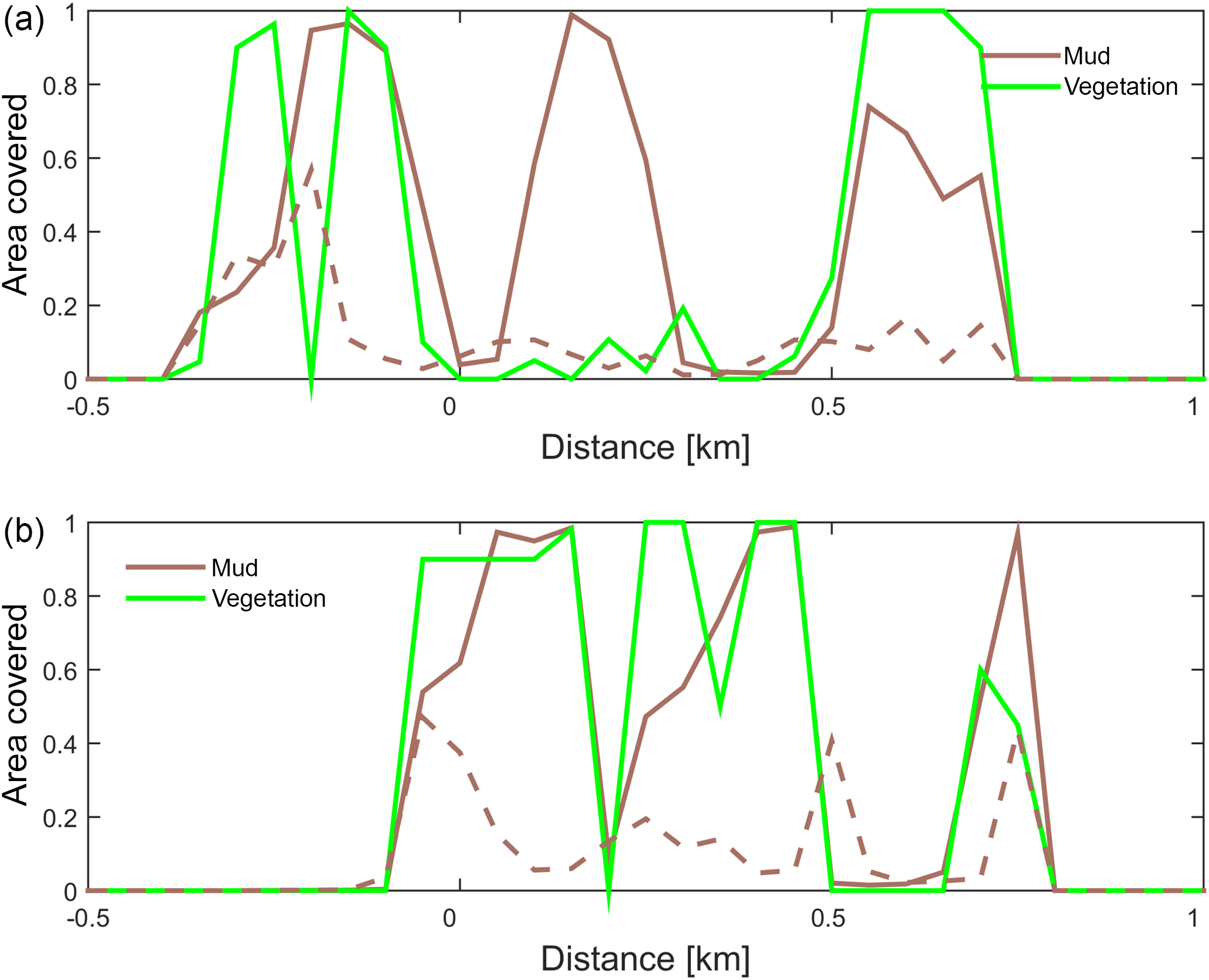
Figure 10Positive feedback between vegetation and mud shown on cross sections through the estuary at (a) 6 km and (b) 8.5 km from the shoreline. The fraction of area covered by mud and by vegetation is plotted for the simulation with only mud (dashed line) and with both mud and vegetation (solid lines).
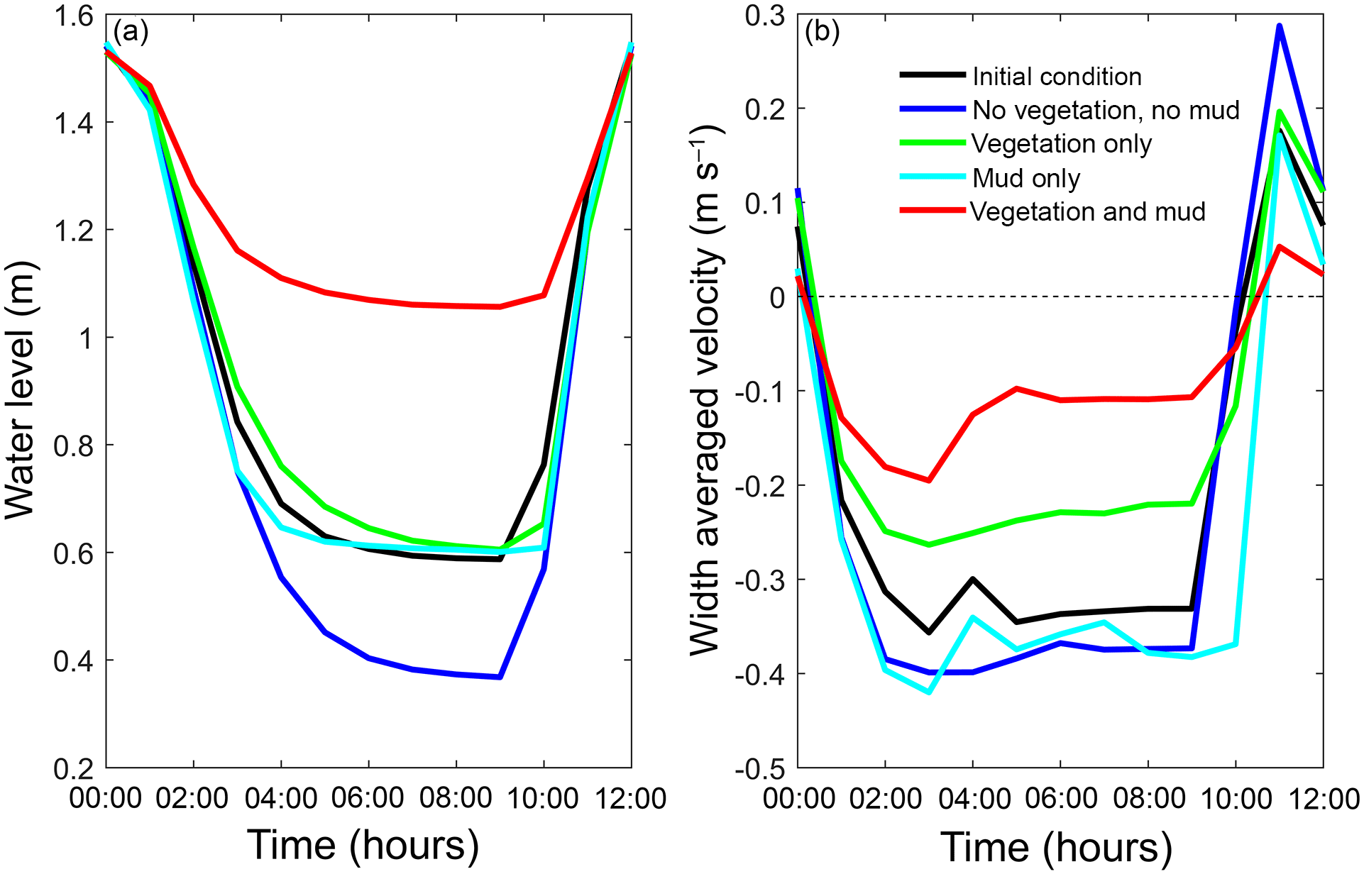
Figure 11The final tidal cycle in the central estuary at 6 km from the mouth, showing the strongest reduction for the scenario with combined mud and vegetation. (a) Tidal water level. (b) Width-averaged flow velocities over the cycle.
Vegetation presence affects the location and thickness of mud deposits mainly in the central estuary (Fig. 7b) and to a lesser degree in the outer area (Fig. 8). The vegetation cover develops faster than the mud cover but afterwards stimulates the mud sedimentation, which reaches a higher final area (Fig. 7). A major difference in hypsometry is, however, that the outer estuary has a concave profile while the central and river reach have a convex profile. This has direct consequences for the available area for vegetation. Because the effect of vegetation is largest in the central part of the estuary, a series of close-up images is provided (Fig. 9). The bathymetry of the reference simulation shows limited changes (Fig. 9a). Vegetation colonises the edges of the area in the simulation without mud but remains distal from the main ebb channel, and the bathymetry develops similar to that of the reference simulation (Fig. 9c). Larger differences occur in simulations where mud is present. When mud is added to the simulation, it first focusses the main ebb channel, but afterwards the entire area starts to gradually fill and becomes shallower (Fig. 9b).
The combined effect of vegetation and mud in the central estuary is to raise the intertidal areas and deepen the subtidal areas relative to the run with mud alone, but the overall depth compared to the control run and vegetation run is reduced. This means that the vegetation acts to focus flow into the channels, but the dominant effect is the filling of intertidal area that reduces the overall tidal prism over time. In the simulation with mud and vegetation, the deeper parts of the estuary no longer accrete. Instead the vegetation captures mud in the intertidal area, and the vegetation expands laterally towards the main channel while focusing the flow (Fig. 9d). Vegetation traps the mud in the higher intertidal areas and through this redistribution decreases the siltation of the deeper parts of the estuary. Simultaneously the accumulation of mud increases the bed level in the central part of the estuary, which enables the vegetation to laterally expand in the direction of the channel. Because mud enables vegetation to expand laterally and because mud accumulation increases within vegetated areas, the total mud and vegetation cover increases when both are present (Fig. 10). Also, the vegetation causes the deposition of mud on bars in the middle of the estuary (Fig. 9d) where mud barely occurs when vegetation is absent (Figs. 9c, 10).
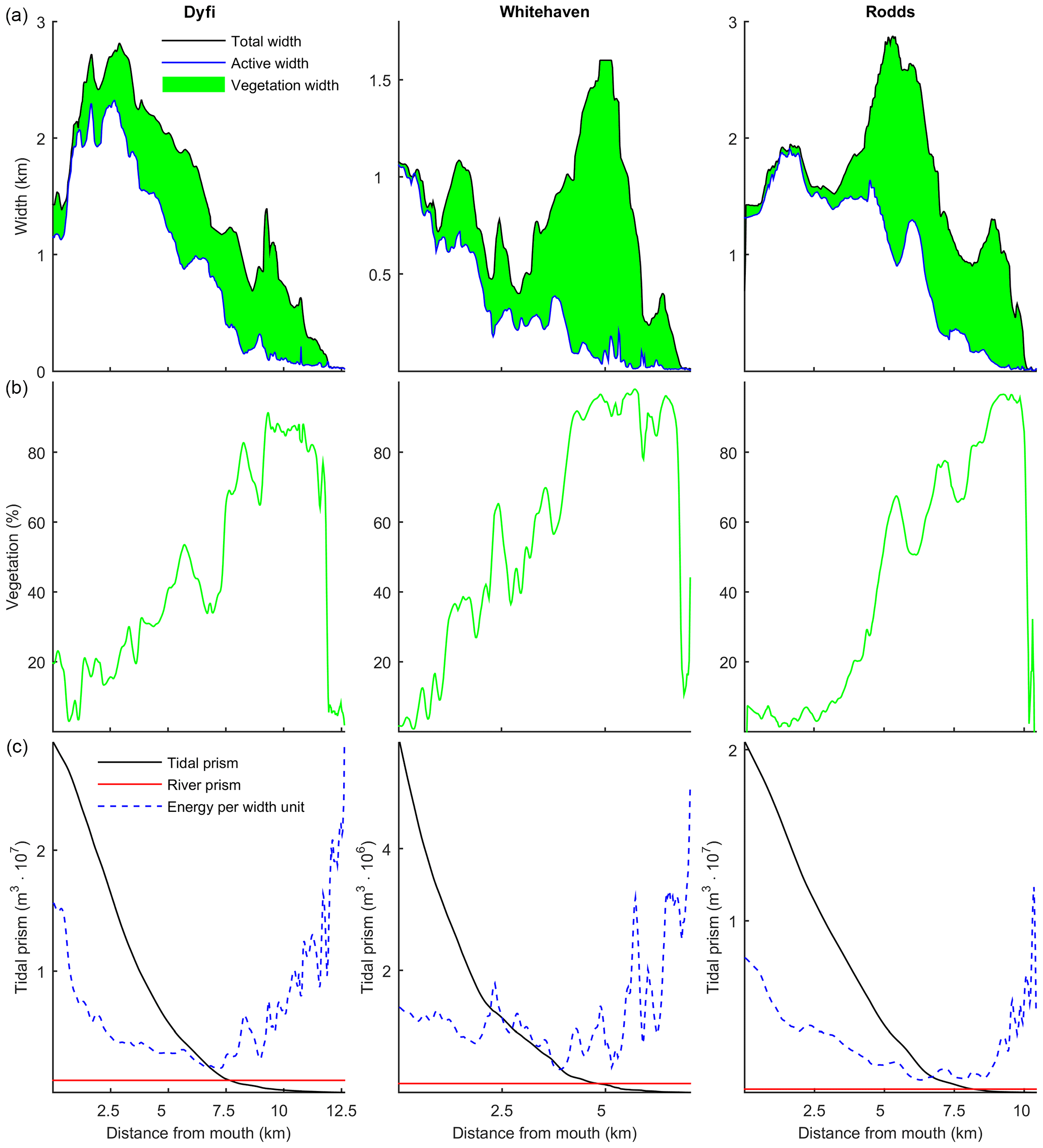
Figure 12(a) The total, active and marsh width along three natural estuaries, partitioned by the method of Leuven et al. (2017). (b) The vegetated part as a percentage of the total width. (c) Tidal prism, discharge and energy taken as width-averaged tidal prism (Leuven et al., 2017).
The water elevation and mean flow velocity in the middle of the estuary were plotted over time to test the hypothesis that the system becomes flood dominant when vegetation (and mud) are present (Fig. 11). The system is ebb dominant from the start. The peak flow velocities occur roughly 1 h before low and high water, and thus the tidal velocity is slightly out of phase. The rise of the tide occurs somewhat faster than the fall of the tide. Normally this would result in higher flood velocities, but in the mixed-energy zone of the estuary they are compensated for by the river discharge. The tidal asymmetry does not change much over time for the four scenarios, but the tidal range decreases for the scenario with mud and vegetation and both simulations with vegetation cause a decreased average flow velocity (Fig. 11b). Furthermore, the effect of combined vegetation and mud is disproportionally larger than that of vegetation or mud alone, confirming the idea of interaction. Moreover, the effect of reduction in tidal prism that determines overall flow energy dominates over the effect of reduction in intertidal area that determines the tendency of flood dominance.
3.3 Real estuaries
The model simulations showed that the relative vegetation abundance increases especially in the mixed-energy zone of the estuary. This is in close agreement with observations in nine real estuaries (Table 4). In real estuaries, vegetation increases in abundance from the estuary mouth towards a short distance before the tidal limit, while landward of the tidal limit the vegetation cover decreases quickly towards zero (Fig. 12). Similar to the modelled scenarios, the landward vegetation cover increase coincides with the decrease in the flow energy. The upper limit of the vegetation is slightly beyond the tidal limit, but this is probably because we included old marshes, which are rarely flooded.
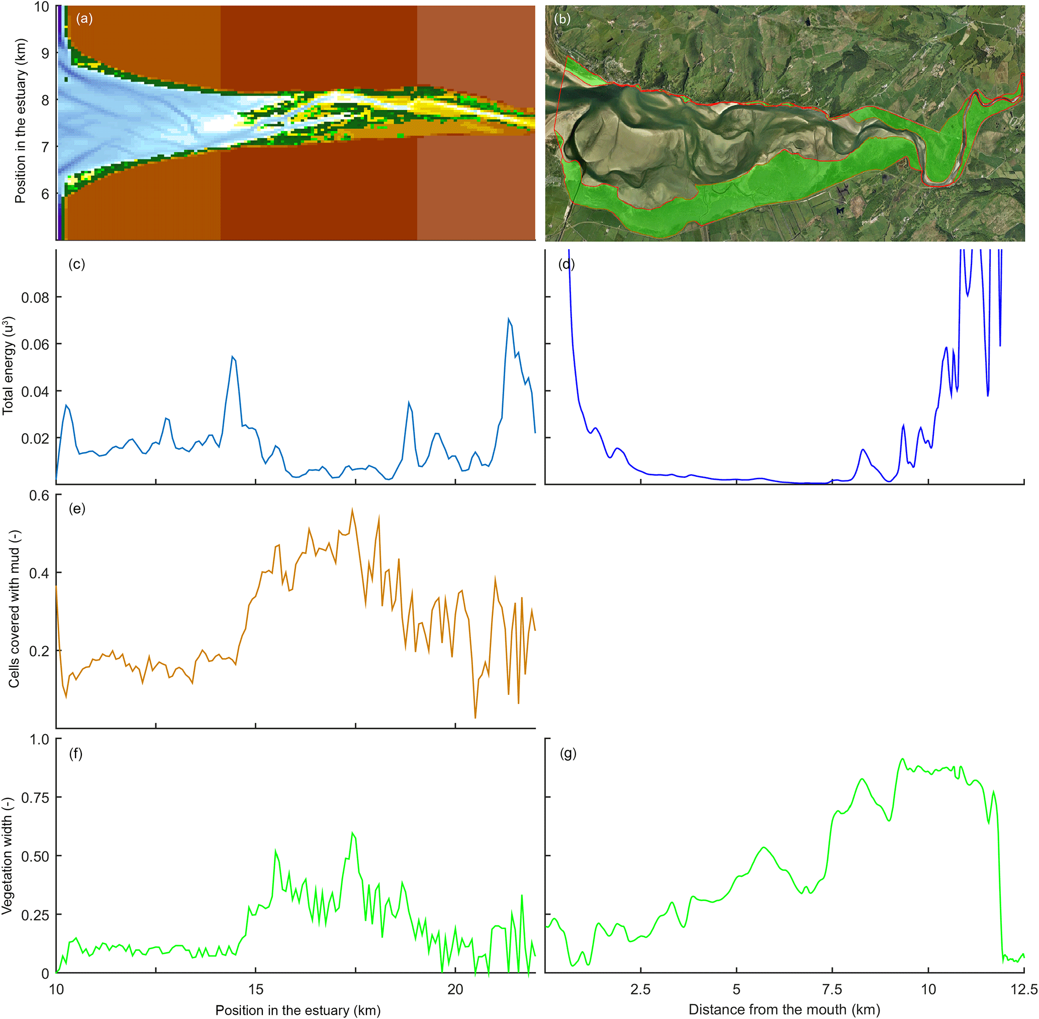
Figure 13Comparison of mudflats and tidal marsh vegetation in a modelled (left) and natural (right) system. Here, velocity magnitude to the power of 3 is plotted as an indication for hydrodynamic energy. Panels (a) and (b) show the estuary bathymetry and vegetation, (c) and (d) show the total energy along the estuary, (e) shows the mud covered area along the estuary, and (f) and (g) show the relative vegetated width of the estuary.
4.1 Marsh distribution
Modelled marshes reach their largest extent in the central estuary, where the tidal energy is the lowest in agreement with the qualitative model of Dalrymple et al. (1992). The tidal marsh expands mostly landward from the maximum flood current velocity. This is also where the bedload convergence zone begins and in natural estuaries where the turbidity maximum zone may occur (Fig. 13). The main reason for the increase in tidal marsh extent is the combination of flow velocities being low enough and the presence of suitable bed elevations. The establishment of tidal marshes requires a window of opportunity with a long enough mild hydrodynamic stress (Bouma et al., 2014). However, the modelled marshes develop primarily landward and not seaward of the maximum flood velocity, which shows that the hydrodynamics are not the only limiting factor. In reality, however, the hydrodynamic stresses will be larger in the outer part and wave magnitude is also more significant there (Dalrymple et al., 1992), and waves are a major limiting factor for seedling establishment in tidal marsh and mangrove landscapes (Balke et al., 2013). Waves would result in a further reduction in tidal marsh extent in the outer estuary but will have limited effect on the central part of the estuary and therefore strengthen the trends in our model.
4.2 Mixed-energy zone
The importance of sediment accumulation in the central part for tidal marsh development is shown in the scenario with mud and vegetation. This simulation shows a further extent of the marshes because mud preferably accumulates in the central part of the estuary, regardless of the fact that no preferential establishment of vegetation on a muddy substrate is included in the model. While it is known that suspended sediment is a requirement for tidal marshes to keep up with sea level rise (D'Alpaos et al., 2006, 2007; Fagherazzi et al., 2012; Murray et al., 2008), the present model results show that suspended sediment is also a requirement for significant lateral marsh progradation into the estuary. We show that the presence of vegetation increases the mud deposition in the upper intertidal area in agreement with observations (Follett and Nepf, 2012; Larsen et al., 2007; Zong and Nepf, 2011), but also that this reduces accumulation in the lower intertidal area. Once the vegetation starts to expand and approaches the main channel (Fig. 9), it starts to focus and concentrate the flow (Fig. 3). After vegetation settlement and stabilisation, vegetation causes flow focusing, similar to the fluvial environment (Dijk et al., 2013; Tal and Paola, 2007).
Despite the reduction in intertidal flood storage, the central zone barely becomes more flood dominant and the tidal limit shifts seaward. This is in contrast to expected tidal dynamics (Friedrichs, 2010), probably because the river in this part of the estuary already dominates over the tidal influence. The seaward shift of the tidal limit implies that the inundation time, and therefore stress, of the marshes decreases, explaining why vegetation density increases in the central estuary. Regardless, the river flow, if large enough to move sediment, will keep a channel open even if the floodplains fill up, such that an equilibrium tidal river may develop. This amounts to progradational filling of the estuary as observed in the Holocene (de Haas et al., 2017).
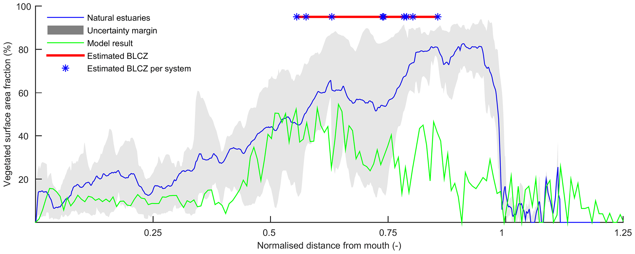
Figure 14Relative vegetated width along the estuary averaged for nine natural estuaries compared to the simulation with mud and vegetation. Distance along the estuary is normalised by the approximate distance between coastline and tidal limit. The approximate location of the bedload convergence zone (BLCZ) is determined by the diminishing of the river energy. The uncertainty margin consists of the 20th and 80th percentile.
4.3 Real estuaries
The general agreement between trends in real estuaries and the numerical model indicates that the overall pattern of tidal marsh and mudflats along the estuary is determined mainly by the tidal hydromorphodynamics and the interaction with mud and vegetation. Figure 14 shows the mean relative vegetation abundance for nine alluvial systems along the tidal–fluvial transition with pronounced marshes. The relative extent of the vegetation can be higher in real estuaries, which has three main causes. First, the modelled system started as a narrow convergent estuary while many real estuaries start from unfilled basins. This leads to the question of whether the pattern of vegetation abundance and the tendency to accumulate sediment in the central estuary would have occurred for other initial conditions. The model results of Braat et al. (2017) show that mud generally settles in similar patterns over most of the modelled period and for most mud concentrations, suggesting that vegetation likewise would have formed similar patterns and central estuary sedimentation. Differences in patterns arise in conditions with very different boundary conditions as discussed below. Second, real estuaries are to a much larger degree infilling than our ebb-dominant system with little sediment import from the sea, and they had a much longer time to fill gradually. Third, many natural estuaries develop pronounced TMZs under influence of density-driven currents, tidal currents and river discharge. Such a TMZ would develop roughly in the mixed-energy zone, and a pronounced TMZ can be hypothesised to enhance accretion and tidal marsh expansion of the central part of the estuary that already occurs without a turbidity maximum zone (Braat et al., 2017).
Our model study simplifies real estuaries in several aspects. First, sediment supply coming from the sea could enhance tidal marsh establishment in the outer estuary. On the other hand, the presence of waves would reduce vegetation survival mainly in the outer estuary where waves are most powerful. Third, the absence of multiple tidal components may reduce the ebb dominance and also limit vegetation development further upstream due to the absence of wetting and drying. Ebb dominance may arise due to the interaction of multiple tidal components which interact and result in a skewed velocity and thus ebb or flood dominance. In our model, there is only velocity asymmetry due to friction-induced lags as a function of tidal stage similar to the process described by Friedrichs (2010). The strongest driver of tidal asymmetry in the central zone is, however, the river discharge. River discharge is known to affect velocity skewness and the timing of slack water and appears to be dominant in the central zone of the estuary (Nidzieko and Ralston, 2012). Fourth, the salinity gradient is ignored, the vegetation along the entire estuary is the same and there are no changes in how vegetation affects hydromorphodynamics along the estuary. While it is not yet known whether typical marsh species along the salinity gradient have different eco-engineering traits which significantly differently affect the long-term morphodynamics, our model is a new tool that, in further research, may lead to new insights in such patterns emerging along the estuary. Regardless, enhanced sedimentation would not change the conclusions, which is that the fundamental feedback mechanism between mud and vegetation affects the larger-scale estuary development: mud facilitates the expansion and survival of marshes while vegetation facilitates the capture of mud, especially in the mixed fluvial–tidal zone.
Numerical modelling of estuaries shows that vegetation follows mud accumulation patterns and simultaneously enhances mud accumulation rates. A positive feedback mechanism emerged in the model between the mud sedimentation and vegetation settlement. Mud sedimentation leads to higher elevated intertidal areas suitable for vegetation settling and development. The vegetation then increases local flow resistance which enhances the sedimentation of mud that would otherwise be resuspended again.
Through this biomorphological feedback loop vegetation has a strong effect on morphodynamics in the middle estuary while its effect in the outer estuary is marginal due to larger flow energy. The relative extent of tidal marsh vegetation increases from the outer estuary towards the inner estuary and can increase from 10 % to 50 % of the estuary width or probably even more, which is in agreement with observations in real estuaries. In particular, the feedback enhances the sedimentary trend in what has been recognised in the literature as the bedload convergence zone in the mixed-energy tidal–fluvial transition. The main effect of the overall intertidal space filling is to reduce the tidal prism and progressively fill the estuary in agreement with observations of Holocene systems. The focusing of flow between flanking marsh vegetation has only a limited effect on channel depth, in contrast to observed effects in salt marsh channels and rivers. The reduction in flood storage has a negligible effect on the flood dominance of the estuary, in contrast to idealised modelling results in the literature, also because the river inflow more than balances the tidal velocity skewness. These results are mainly valid for shallow sandy estuaries.
The effect of vegetation alone on the hypsometry of the entire estuary is limited. This is mainly because its effect on the outer estuary is marginal, where it occupies only a small portion of the estuary surface. In the central part of the estuary, vegetation occupies a much larger fraction of the width so that its effects are most pronounced here. When mud is present and forms a new intertidal area, the vegetation expands towards the channel, which drives further accretion and forces the system into a single main channel. When mud is absent vegetation lacks an accreting effect because the sand does not reach the vegetated areas for lack of energy in the shallowest flows. This means that the greatest morphological effects of vegetation and mud emerge when they occur simultaneously as they have mutual positive feedbacks. The combined presence of mud and vegetation leads to the focusing of flow and channel incision on a decadal timescale but may lead to the infilling of the estuary on a centennial timescale due to the accumulation of the intertidal area and the consequent reduction in the tidal prism.
Any data in this paper were derived by numerical modelling that can be repeated with the open-source code of the model.
The authors contributed in the following proportions to conception and design, data collection, modelling, analysis and conclusions, and manuscript preparation: IRL (40 %, 50 %, 70 %, 60 %, 70 %), LB (10 %, 0 %, 10 %, 0 %, 0 %), JRFWL (0 %, 50v, 0 %, 0 %, 0 %), AWB (0 %, 0 %, 0 %, 0 %, 10 %), MvO (0 %, 0 %, 10 %, 0 %, 0 %), SS (20 %, 0 %, 10 %, 20 %, 0 %), MGK (30 %, 0 %, 0 %, 20 %, 10 %).
The authors declare that they have no conflict of interest.
Ivar R. Lokhorst, Sanja Selaković and Maarten G. Kleinhans were supported by the European Research Council (ERC Consolidator agreement 647570) to
PI Maarten G. Kleinhans. Lisanne Braat, Jasper R. F. W. Leuven, Anne W. Baar and Maarten G. Kleinhans were supported by the Dutch Technology Foundation STW (part of the
Netherlands Organisation for Scientific Research, grant Vici 016.140.316/13710) to PI Maarten G. Kleinhans. Mijke van Oorschot was
supported by REFORM (FP7 grant agreement). We would like to thank Eli Lazarus and the anonymous reviewers
for their contributions to improving the paper. Model support by Deltares is gratefully acknowledged. The
modelling was a continuation of the MSc thesis of Ivar R. Lokhorst supervised by Sanja Selaković and Maarten G. Kleinhans.
Edited by: Orencio Duran Vinent
Reviewed by: Eli D. Lazarus and two anonymous referees
Allen, J.: A continuity-based sedimentological model for temperate-zone tidal salt marshes, J. Geol. Soc., 151, 41–49, 1994. a
Aubrey, D. and Speer, P.: A study of non-linear tidal propagation in shallow inlet/estuarine systems Part I: Observations, Estuar. Coast. Shelf Sci., 21, 185–205, 1985. a
Balke, T., Webb, E. L., den Elzen, E., Galli, D., Herman, P. M., and Bouma, T. J.: Seedling establishment in a dynamic sedimentary environment: a conceptual framework using mangroves, J. Appl. Ecol., 50, 740–747, 2013. a
Baptist, M., Babovic, V., Rodríguez Uthurburu, J., Keijzer, M., Uittenbogaard, R., Mynett, A., and Verwey, A.: On inducing equations for vegetation resistance, J. Hydraul. Res., 45, 435–450, 2007. a, b
Bouma, T., Vries, M. D., Low, E., Kusters, L., Herman, P., Tanczos, I., Temmerman, S., Hesselink, A., Meire, P., and Van Regenmortel, S.: Flow hydrodynamics on a mudflat and in salt marsh vegetation: identifying general relationships for habitat characterisations, Hydrobiologia, 540, 259–274, 2005. a
Bouma, T., Van Duren, L., Temmerman, S., Claverie, T., Blanco-Garcia, A., Ysebaert, T., and Herman, P.: Spatial flow and sedimentation patterns within patches of epibenthic structures: Combining field, flume and modelling experiments, Cont. Shelf Res., 27, 1020–1045, 2007. a
Bouma, T. J., van Belzen, J., Balke, T., Zhu, Z., Airoldi, L., Blight, A. J., Davies, A. J., Galvan, C., Hawkins, S. J., Hoggart, S. P., Lara, J. L., Losada, I. J., Maza, M., Ondiviela, B., Skov, M. W., Strain, E. M., Thompson, R. C., Yang, S., Zanuttigh, B., Zhang, L., and Herman, P. M. J.: Identifying knowledge gaps hampering application of intertidal habitats in coastal protection: Opportunities & steps to take, Coast. Eng., 87, 147–157, https://doi.org/10.1016/j.coastaleng.2013.11.014, 2014. a
Braat, L., van Kessel, T., Leuven, J. R. F. W., and Kleinhans, M. G.: Effects of mud supply on large-scale estuary morphology and development over centuries to millennia, Earth Surf. Dynam., 5, 617–652, https://doi.org/10.5194/esurf-5-617-2017, 2017. a, b, c, d, e, f, g, h, i, j, k, l, m, n, o, p, q
Brenon, I. and Le Hir, P.: Modelling the turbidity maximum in the Seine estuary (France): identification of formation processes, Estuar. Coast. Shelf Sci., 49, 525–544, 1999. a
Brew, D. S. and Williams, P. B.: Predicting the impact of large-scale tidal wetland restoration on morphodynamics and habitat evolution in south San Francisco Bay, California, J. Coast. Res., 26, 912–924, 2010. a
Burge, L. M.: Wandering Miramichi rivers, New Brunswick, Canada, Geomorphology, 69, 253–274, 2005. a
Coco, G., Zhou, Z., van Maanen, B., Olabarrieta, M., Tinoco, R., and Townend, I.: Morphodynamics of tidal networks: advances and challenges, Mar. Geol., 346, 1–16, 2013. a
Corenblit, D., Steiger, J., Gurnell, A. M., and Naiman, R. J.: Plants intertwine fluvial landform dynamics with ecological succession and natural selection: a niche construction perspective for riparian systems, Global Ecol. Biogeogr., 18, 507–520, 2009. a, b
D'Alpaos, A., Lanzoni, S., Mudd, S. M., and Fagherazzi, S.: Modeling the influence of hydroperiod and vegetation on the cross-sectional formation of tidal channels, Estuar. Coast. Shelf Sci., 69, 311–324, 2006. a, b, c
D'Alpaos, A., Lanzoni, S., Marani, M., and Rinaldo, A.: Landscape evolution in tidal embayments: modeling the interplay of erosion, sedimentation, and vegetation dynamics, J. Geophys. Res.-Earth, 112, https://doi.org/10.1029/2006JF000537, 2007. a
Dalrymple, R. W., Zaitlin, B. A., and Boyd, R.: Estuarine facies models: conceptual basis and stratigraphic implications: perspective, J. Sediment. Res., 62, 1130–1146, https://doi.org/10.1306/D4267A69-2B26-11D7-8648000102C1865D, 1992. a, b, c, d, e, f, g, h
Darby, S. E.: Effect of riparian vegetation on flow resistance and flood potential, J. Hydraul. Eng., 125, 443–454, 1999. a
Davidson, N., Laffoley, D. D., Doody, J., Way, L., Gordon, J., Key, R. E., Drake, C., Pienkowski, M., Mitchell, R., and Duff, K.: Nature conservation and estuaries in Great Britain, Nature Conservancy Council, Peterborough, 1–76, 1991. a
de Haas, T., Pierik, H., van der Spek, A., Cohen, K., van Maanen, B., and Kleinhans, M.: Holocene evolution of tidal systems in the Netherlands: effects of rivers, coastal boundary conditions, eco-engineering species, inherited relief and human interference, Earth-Sci. Rev., 177, 139–163, https://doi.org/10.1016/j.earscirev.2017.10.006, 2017. a, b
Deng, Z., Deng, Z., An, S., Wang, Z., Liu, Y., Ouyang, Y., Zhou, C., Zhi, Y., and Li, H.: Habitat choice and seed–seedling conflict of Spartina alterniflora on the coast of China, Hydrobiologia, 630, 287–297, 2009. a, b, c
Dijk, W., Teske, R., Lageweg, W., and Kleinhans, M.: Effects of vegetation distribution on experimental river channel dynamics, Water Resour. Res., 49, 7558–7574, 2013. a, b, c
Fagherazzi, S., Kirwan, M. L., Mudd, S. M., Guntenspergen, G. R., Temmerman, S., D'Alpaos, A., Koppel, J., Rybczyk, J. M., Reyes, E., Craft, C., and Clough, J.: Numerical models of salt marsh evolution: Ecological, geomorphic, and climatic factors, Rev. Geophys., 50, https://doi.org/10.1029/2011RG000359, 2012. a
Ferguson, R.: Hydraulic and sedimentary controls of channel pattern, in: River channels: environment and process, edited by: Richards, K., Inst. British Geographers Special Publication 18, 129–158, Blackwell, Oxford, UK, 1987. a
Follett, E. M. and Nepf, H. M.: Sediment patterns near a model patch of reedy emergent vegetation, Geomorphology, 179, 141–151, 2012. a
French, J. R.: Numerical simulation of vertical marsh growth and adjustment to accelerated sea-level rise, north Norfolk, UK, Earth Surf. Proc. Land., 18, 63–81, 1993. a
Friedrichs, C. T.: Barotropic tides in channelized estuaries, Contemporary Issues in Estuarine Physics, 27–61, 2010. a, b, c, d
Friedrichs, C. T. and Perry, J. E.: Tidal salt marsh morphodynamics: a synthesis, J. Coast. Res., 27, 7–37, 2001. a, b
Gurnell, A. M., Bertoldi, W., and Corenblit, D.: Changing river channels: The roles of hydrological processes, plants and pioneer fluvial landforms in humid temperate, mixed load, gravel bed rivers, Earth-Sci. Rev., 111, 129–141, 2012. a
Järvelä, J.: Flow resistance of flexible and stiff vegetation: a flume study with natural plants, J. Hydrol., 269, 44–54, 2002. a
Johnson, M., Kenyon, N., Belderson, R., and Stride, A.: Offshore Tidal Sands, Processes and Deposits, chap. Sand transport, Chapman and Hall, London, 1982. a
Kirwan, M. and Temmerman, S.: Coastal marsh response to historical and future sea-level acceleration, Quaternary Sci. Rev., 28, 1801–1808, 2009. a
Kleinhans, M., de Vries, B., and van Oorschot, M.: Effects of mud on the morphodynamic development of a modelled river, Earth Surf. Proc. Land., https://doi.org/10.1002/esp.4437, 2018. a, b
Larsen, L. G., Harvey, J. W., and Crimaldi, J. P.: A delicate balance: ecohydrological feedbacks governing landscape morphology in a lotic peatland, Ecol. Monogr., 77, 591–614, 2007. a
Lee, W. G. and Partridge, T. R.: Rates of spread of Spartina anglica and sediment accretion in the New River Estuary, Invercargill, New Zealand, New Zeal. J. Bot., 21, 231–236, 1983. a
Leuven, J., Haas, T., Braat, L., and Kleinhans, M.: Topographic forcing of tidal sand bar patterns for irregular estuary planforms, Earth Surf. Proc. Land., https://doi.org/10.1002/esp.4166, 2017. a, b, c, d, e, f, g
Marani, M., Da Lio, C., and D'Alpaos, A.: Vegetation engineers marsh morphology through multiple competing stable states, P. Natl. Acad. Sci. USA, 110, 3259–3263, 2013. a
Meire, P., Ysebaert, T., Van Damme, S., Van den Bergh, E., Maris, T., and Struyf, E.: The Scheldt estuary: a description of a changing ecosystem, Hydrobiologia, 540, 1–11, 2005. a
Mudd, S. M., D'Alpaos, A., and Morris, J. T.: How does vegetation affect sedimentation on tidal marshes? Investigating particle capture and hydrodynamic controls on biologically mediated sedimentation, J. Geophys. Res.-Earth, 115, https://doi.org/10.1029/2009JF001566, 2010. a
Murray, A., Knaapen, M., Tal, M., and Kirwan, M.: Biomorphodynamics: Physical-biological feedbacks that shape landscapes, Water Resour. Res., 44, https://doi.org/10.1029/2007WR006410, 2008. a
Nehring, S. and Adsersen, H.: NOBANIS–Invasive Alien Species Fact Sheet Spartina anglica, From: Online Database of the North European and Baltic Network on Invasive Alien Species–NOBANIS, available at: https://www.artportalen.se/nobanis (last access: 1 January 2018), 2006. a, b, c, d
Nidzieko, N. J. and Ralston, D. K.: Tidal asymmetry and velocity skew over tidal flats and shallow channels within a macrotidal river delta, J. Geophys. Res.-Oceans, 117, C03001, https://doi.org/10.1029/2011JC007384, 2012. a
Oorschot, M. V., Kleinhans, M., Geerling, G., and Middelkoop, H.: Distinct patterns of interaction between vegetation and morphodynamics, Earth Surf. Proc. Land., https://doi.org/10.1002/esp.3864, 2015. a, b, c, d, e, f, g, h, i
Orson, R., Panageotou, W., and Leatherman, S. P.: Response of tidal salt marshes of the US Atlantic and Gulf coasts to rising sea levels, J. Coast. Res., 1, 29–37, 1985. a
Partheniades, E.: Erosion and deposition of cohesive soils, J. Hydr. Div.-ASCE, 91, 105–139, 1965. a
Redfield, A. C.: Development of a New England salt marsh, Ecol. Monogr., 42, 201–237, 1972. a
Schuurman, F., Marra, W. A., and Kleinhans, M. G.: Physics-based modeling of large braided sand-bed rivers: Bar pattern formation, dynamics, and sensitivity, J. Geophys. Res.-Earth, 118, 2509–2527, 2013. a
Siniscalchi, F., Nikora, V. I., and Aberle, J.: Plant patch hydrodynamics in streams: Mean flow, turbulence, and drag forces, Water Resour. Res., 48, https://doi.org/10.1029/2011WR011050, 2012. a
Speer, P. and Aubrey, D.: A study of non-linear tidal propagation in shallow inlet/estuarine systems Part II: Theory, Estuar. Coast. Shelf Sci., 21, 207–224, 1985. a
Tal, M. and Paola, C.: Dynamic single-thread channels maintained by the interaction of flow and vegetation, Geology, 35, 347–350, 2007. a, b
Temmerman, S., Bouma, T., Van de Koppel, J., Van der Wal, D., De Vries, M., and Herman, P.: Vegetation causes channel erosion in a tidal landscape, Geology, 35, 631–634, 2007. a
Townend, I., Fletcher, C., Knappen, M., and Rossington, K.: A review of salt marsh dynamics, Water Environ. J., 25, 477–488, 2011. a
Van der Wegen, M. and Roelvink, J.: Long-term morphodynamic evolution of a tidal embayment using a two-dimensional, process-based model, J. Geophys. Res.-Oceans, 113, https://doi.org/10.1029/2006JC003983, 2008. a
Zong, L. and Nepf, H.: Spatial distribution of deposition within a patch of vegetation, Water Resour. Res., 47, https://doi.org/10.1029/2010WR009516, 2011. a