Can the growth of deltaic shorelines be unstable?

We study a sedimentary delta prograding over a fixed adversely sloping bathymetry, asking whether a perturbation to the advancing shoreline will grow (unstable) or decay (stable) through time. To start, we use a geometric model to identify the condition for acceleration of the shoreline advance (auto-acceleration). We then model the growth of a delta on to a fixed adverse bathymetry, solving for the speed of the shoreline as a function of the water depth, foreset repose angle, fluvial top set slope, and shoreline curvature. Through a linearization of this model, we arrive at a stability criterion for a delta shoreline, indicating that auto-acceleration is a necessary condition for unstable growth. This is the first time such a shoreline instability has been identified and analyzed. We use the derived stability criterion to identify a characteristic lateral length scale for the shoreline morphology resulting from an unstable growth. On considering experimental and field conditions, we observe that this length scale is typically larger than other geomorphic features in the system, e.g., channel spacings and dimensions, suggesting that the signal of the shoreline growth instability in the landscape might be “shredded” by other surface building processes, e.g., channel avulsions and alongshore transport.

1 Introduction

Shorelines are the moving boundary between land and sea, and their evolution is of great importance to the estimated 10% of the global population that live in their proximity (Wong et al., 2014). Shorelines are also an area of scientific interest because their shape records information about the processes that formed them. While significant progress has been made in characterizing shoreline shape (Shaw et al., 2008; Geleynse et al., 2012), inferring formative processes from shoreline shape remains a challenge. Galloway (1975) recognized that qualitatively, the shape of a delta shoreline reflects the relative importance of waves, tides, and fluvial input, but using shoreline shape to assess the strength of these processes quantitatively remains an open challenge (Nienhuis et al., 2015; Baumgardner, 2016). Part of the challenge may lie in the susceptibility of shorelines to instabilities. For example, an instability associated with high-angle waves results in the self-organization of regular, quasiperiodic shoreline features (Ashton and Murray, 2006). Another type of instability important for deltaic shorelines is the channel-forming instability. Although unchannelized sheet flow can be observed in nature on some alluvial fans, channelized flow is more common. This has been ascribed to the instability of sheet flow, tending to evolve towards a channelized state (Whipple et al., 1998). This instability can be expected to manifest itself in the shape of the shoreline, with areas near channels receiving the most sediment and therefore prograding faster relative to the rest of the shoreline.

Here our interest will focus on a new mechanism that might drive the instability of an advancing delta shoreline. Our motivation is the recent works from Hajek et al. (2014) and López et al. (2014), who have studied the growth of a sedimentary delta under a condition of a “back-tilted” subsidence rate, a condition that resulted in the water depth ahead of the shoreline decreasing with distance (i.e., the delta builds on an adverse slope). Such scenarios can arise in foreland basins where the sediment supply is sufficiently high relative to subsidence for progradation to occur if a prograding delta approaches the opposite side of a lake or reservoir or if the delta toe encounters an adverse slope on an offshore bar. In a one-dimensional modeling and experimental study, López et al. (2014) indicated that, for some combinations of sediment input and subsidence style, delta progradation on an adverse slope could exhibit a positive acceleration, referred to as “auto-acceleration”. We think that such a behavior could be a critical ingredient for the onset of unstable growth. To see this, imagine a two-dimensional growth scenario, in plan view, with an advancing planar shoreline front. Under an auto-accelerating regime any “blip” (perturbation) in the growth direction along the shoreline front could find itself in a location which is more favorable for growth. In this way, it is possible that, under the right conditions, rather than being consumed by the advancing planar shoreline, this blip will accelerate away and provide a potential driver for an unstable morphological breakdown of the planar shoreline. Indeed, the two-dimensional delta growth experiments from Hajek et al. (2014) underscore this possibility by observing “a tendency for shorelines to run away seaward in response to base-level fall in back-tilted basins”.

In exploring the possible instability associated with auto-acceleration, we will appeal to the analogy between solid and liquid phase change processes and delta shoreline advance (Swenson et al., 2000; Voller et al., 2004; Capart et al., 2007; Lorenzo-Trueba et al., 2009; Voller, 2010; Ke and Capart, 2015; Lai et al., 2017). This analogy is based on the construction of a shoreline mass balance condition, equating the sediment flux arriving to the rate of its advance – a condition directly analogous to the phase change interface heat balance Stefan condition in melting problems (Crank, 1984). The original shore balance proposed by Swenson et al. (2000) has been recently modified by Ke and Capart (2015) to account for the shoreline planform curvature. Recognizing the extensive work related to the role of curvature in the morphological instability of growing interfaces (Mullins and Sekerka, 1963; Sekerka et al., 2014; Paterson, 1981; Li et al., 2004, 2009; Zhao et al., 2016), this modification allows us to expand the so-called Swenson–Stefan analogy to develop a criterion for an unstable delta shoreline advance.

Principally, we are interested in answering a number of key questions.

• Under what conditions would an unstable shoreline growth arise and how would it evolve over time?

• What, if any, is the connection between auto-acceleration an unstable shoreline growth?

• What would the characteristic length scale of the instability be and how does this scale compare to other geomorphic length scales in deltaic shoreline settings, e.g., channel spacings?

To set the stage for our study, we adopt the delta geometry used in the López et al. (2014) model, and then, on invoking the additional simplifying assumption of a static basin with a constant water level, we arrive at an explicit criterion for the onset of auto-acceleration. To see and understand how such a condition may lead to an unstable growth condition, we further perform a linear stability analysis of the Ke and Capart (2015) shoreline condition, identifying the criterion when a specified small perturbation on a planar auto-accelerating shoreline front would be expected to grow, i.e., become unstable.

2 A geometric model

The one-dimensional model recently presented in López et al. (2014) assumed that the growth of a delta into a basin with a back-tilting hinged subsidence rate would, under the supply of a constant unit sediment flux q at the origin x=0, maintain a similar geometry with fixed positive top set (S_T>0) and foreset ($S_{\mathrm{F}}=\tan \left(\mathit{\alpha }\right),\mathit{\alpha }\in [\mathrm{0},\frac{\mathit{\pi }}{\mathrm{2}}]$) slopes. Here we retain these geometric assumptions but invoke an additional assumption that the delta builds onto a basement with a fixed (non-subsiding) slope S_B, a limiting simplification, which allows us to directly arrive at an explicit condition under which auto-acceleration will occur. This geometric model is schematically represented in the cross section (long profile) shown in Fig. 1. If we assume that this schematic is for a one-dimensional planar growing delta, an analysis of the change in area of the deposit cross section due to a small incremental advance of the shoreline x=ℓ(t) leads to the following expression for the shoreline speed

$$\begin{array}{}\text{(1)}& v={\displaystyle \frac{\mathrm{d}\mathrm{\ell }}{\mathrm{d}t}}={\displaystyle \frac{q}{\mathrm{\ell }{S}_{\mathrm{T}}+D}},\end{array}$$

where D is the water depth at the point where the foreset toe meets the basement. The water depth can be determined in two ways: in terms of the foreset length, i.e., D=Lsin (α), or, after appropriate geometric algebra, in terms of the shoreline position, i.e., $D=\frac{\mathrm{\ell }{S}_{\mathrm{B}}+D_{\mathrm{0}}}{\mathrm{1}-\frac{S_{\mathrm{B}}}{S_{\mathrm{F}}}}$, where D₀ is the constant water depth at x=0. On taking a further derivative in time we arrive at an expression for the acceleration of the shoreline:

$$\begin{array}{}\text{(2)}& a={\displaystyle \frac{{\mathrm{d}}^{\mathrm{2}}\mathrm{\ell }}{\mathrm{d}{t}^{\mathrm{2}}}}=-q{\displaystyle \frac{\mathrm{d}\mathrm{\ell }}{\mathrm{d}t}}{\displaystyle \frac{[S_{\mathrm{T}}+\frac{S_{\mathrm{B}}}{\mathrm{1}-\frac{S_{\mathrm{B}}}{S_{\mathrm{F}}}}]}{[\mathrm{\ell }{S}_{\mathrm{T}}+D{]}^{\mathrm{2}}}};\end{array}$$

note $\mathrm{d}D/\mathrm{d}\mathrm{\ell }=\frac{S_{\mathrm{B}}}{\mathrm{1}-S_{\mathrm{B}}/S_{\mathrm{F}}}$. To exhibit auto-acceleration, the value of a will need to be positive, requiring that the numerator in the last term on the right-hand side of Eq. (2) will need to be negative, which, in turn, implies that, under the assumption of a fixed basement, an explicit condition for auto-acceleration can be written as

$$\begin{array}{}\text{(3)}& S_{\mathrm{B}}^{\mathrm{e}}={\displaystyle \frac{S_{\mathrm{B}}}{\mathrm{1}-\frac{S_{\mathrm{B}}}{S_{\mathrm{F}}}}}+S_{\mathrm{T}}<\mathrm{0},\end{array}$$

where we define $S_{\mathrm{B}}^{\mathrm{e}}$ to be an effective basement slope. Note that this condition tells us that, since the top slope, S_T, and foreset slope, S_F, are always positive and S_B<S_F, we will only observe auto-acceleration when the basement slope is adverse; i.e., S_B<0. In fact, after some algebra, we see that for auto-acceleration, we need an adverse basement with an absolute slope value $\left|S_{\mathrm{B}}\right|>b{S}_{\mathrm{T}}$, where the prefactor, which is always positive, $b=(\mathrm{1}-S_{\mathrm{B}}/S_{\mathrm{F}})$. We expect the value of this prefactor to range between 1 when $-S_{\mathrm{B}}\ll S_{\mathrm{F}}$ and ∼2 when the basement and foreset slopes are close in value ($-S_{\mathrm{B}}\sim S_{\mathrm{F}}$).

As we noted above, while meeting the auto-acceleration condition, $S_{\mathrm{B}}^{\mathrm{e}}<\mathrm{0}$ may lead to unstable shoreline growth; it is not clear if the occurrence of auto-acceleration is sufficient for such a behavior. For example, the geometry (e.g., curvature) of a shoreline perturbation on an accelerating front might retard its further growth. In order to arrive at a more rigorous condition for shoreline stability, we need to develop a treatment that can account for planform perturbations of the planar front. Such a treatment will require a more sophisticated model for the partitioning of the sediment between the fluvial and submarine area. To this end, we develop a linear stability analysis for a two-dimensional plan view shoreline that uses the local shoreline mass balance proposed by Ke and Capart (2015).

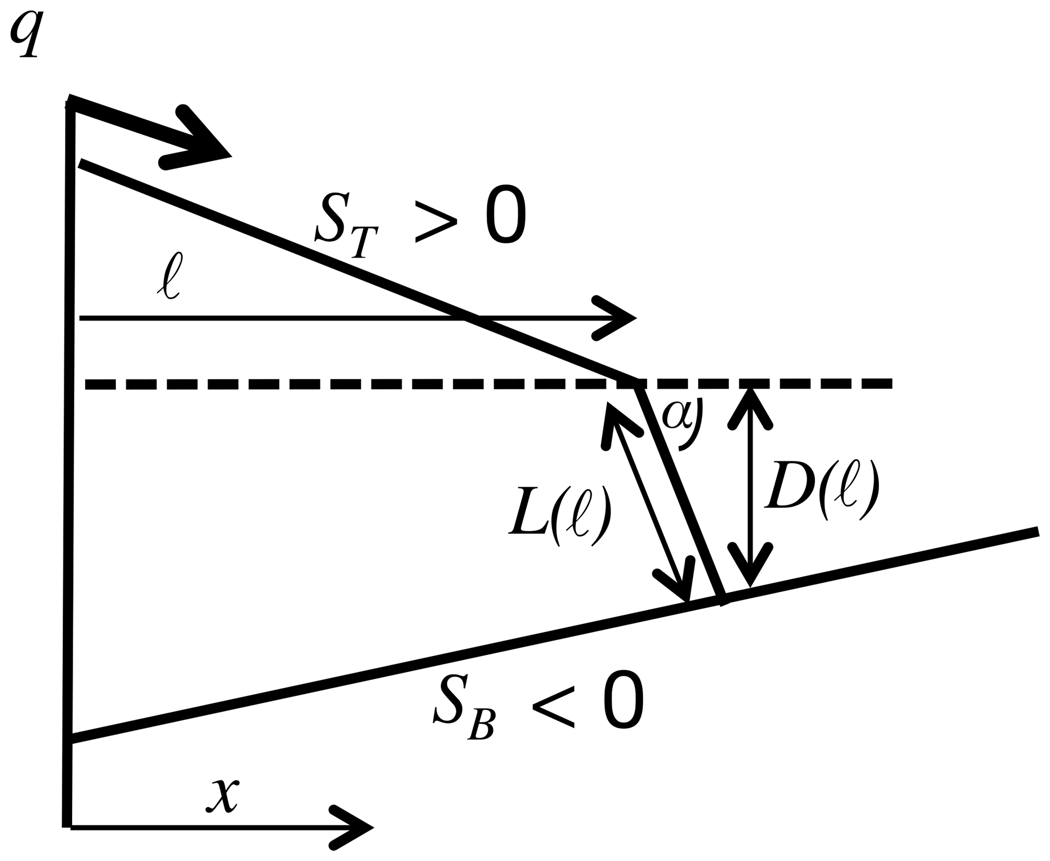
Figure 1 Schematics of sediment delta cross sections depositing on to a fixed basement with an adverse slope S_B<0. The top set slope is S_T>0 and the submarine foreset has angle α, length L(ℓ), and a depth of D(ℓ) at the point where its toe touches the basement.

3 A linear stability analysis

The key ingredient in the analogy (see Swenson et al., 2000) between the advance of a sediment delta front into a standing body water and the tracking of the liquid or solid Stefan melting front is the determination of how the sediment arriving on the land side of the shoreline is deposited into the submarine area. In the one-dimensional Swenson analogy this involves a simple distribution of the excess sediment arriving at the shoreline to maintain a submarine foreset of constant slope (see Fig. 1), a device that leads to a relationship between the speed of the shoreline advance and the land-side sediment supply. The major contribution in the work by Ke and Capart (2015) is to generalize this relationship to a case where the growing delta has a two-dimensional planform (x in the seaward direction and y in the lateral); i.e., from Eq. (23) in Ke and Capart (2015), the shoreline evolves as

$$\begin{array}{}\text{(4)}& {\displaystyle \frac{\partial \mathit{x}}{\partial t}}\cdot \mathit{n}={\displaystyle \frac{\mathbf{J}\cdot \mathit{n}}{\sin \mathit{\alpha }\left(L\right(\mathit{x})+\frac{\mathrm{1}}{\mathrm{2}}\mathit{\kappa }{L}^{\mathrm{2}}(\mathit{x}\left)\cos \mathit{\alpha }\right)}},\end{array}$$

where x is the Cartesian position vector for a point on the shoreline, J⋅n is the unit sediment flux (+ pore space) arriving to the landward side of the shoreline (essentially the excess material that can be used for shoreline advance), n is the seaward pointing unit normal on the shoreline, α is the angle of repose of the foreset, L(x) is its length, and κ is the planform curvature of the shoreline. We will use this more general shoreline condition as the basis for our linear stability analysis.

In the case of a planar shoreline (curvature κ=0) at position x=ℓ(t), under our assumptions of a fixed a fluvial slope and constant unit discharge, $\mathbf{J}\cdot \mathit{n}=q-S_{\mathrm{T}}\mathrm{\ell }\dot{\mathrm{\ell }}$ and the condition in Eq. (4) reduces to

$$\begin{array}{}\text{(5)}& \dot{\mathrm{\ell }}={\displaystyle \frac{q-S_{\mathrm{T}}\mathrm{\ell }\dot{\mathrm{\ell }}}{L\sin \mathit{\alpha }}},\end{array}$$

where $\dot{\mathrm{\ell }}=\partial \mathrm{\ell }/\partial t=v$, the planar front velocity. On recognizing that Lsin α=D, where D is the depth of the foreset toe, we see that this equation can be rearranged as $\dot{\mathrm{\ell }}=v=q/(\mathrm{\ell }{S}_{\mathrm{T}}+D)$, matching our geometric mass balance model in Eq. (1).

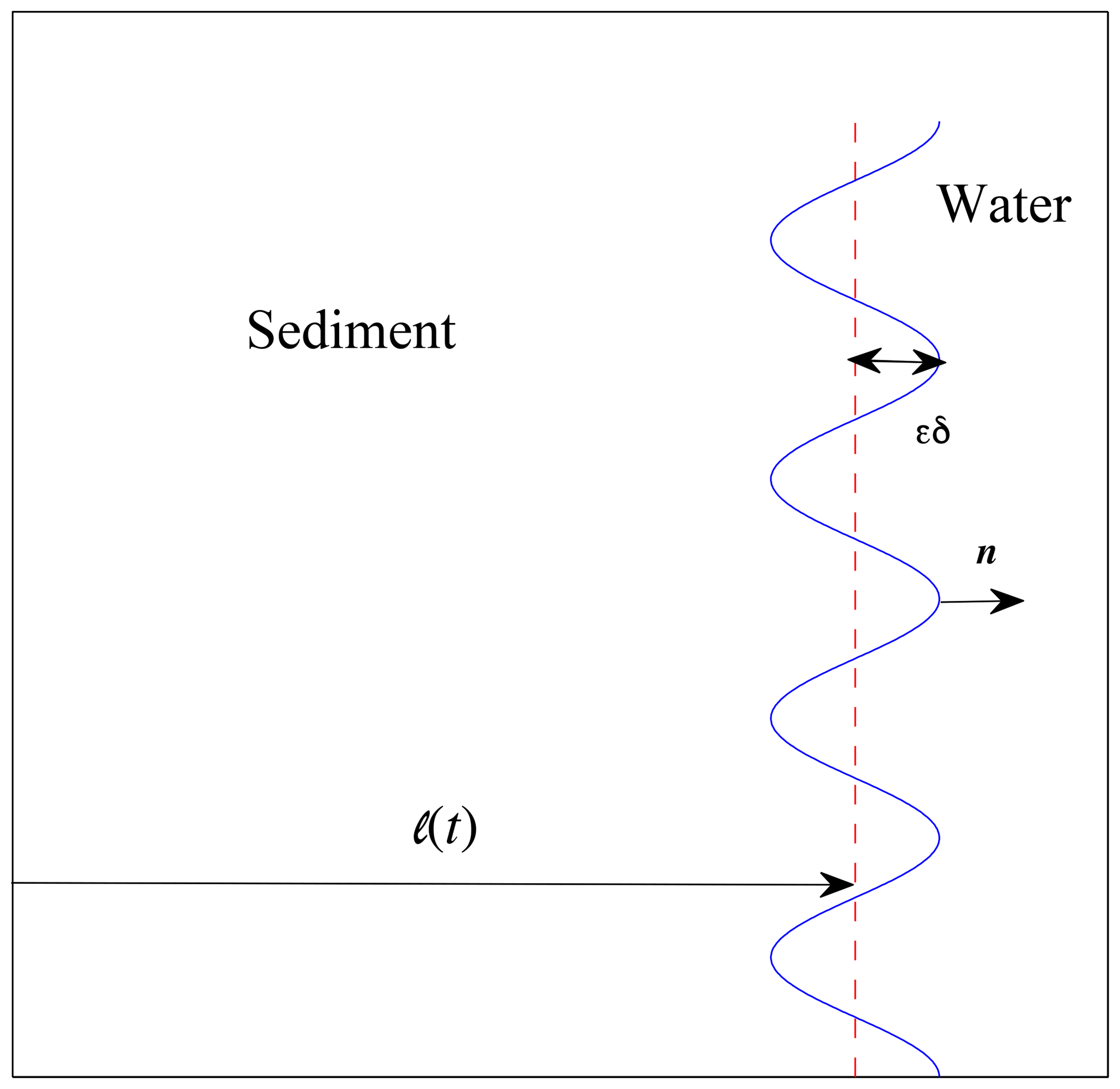
The starting point for our stability analysis is to introduce a small perturbation of the planar front with the form

$$\begin{array}{}\text{(6)}& x(t,y)=\mathrm{\ell }\left(t\right)+\mathit{ϵ}\mathit{\delta }\left(t\right)\cos \left(ky\right),\end{array}$$

where, with reference to Fig. 2, δ(t) is the amplitude of the perturbation, the parameter ϵ≪1, and k is the wave number, related to the wavelength of the perturbation through $\mathit{\lambda }=\mathrm{2}\mathit{\pi }/k$. This step allows us to ask whether a small perturbation to the shoreline will shrink back to the advancing front (stable) or if it will accelerate away from it (unstable)? With the given perturbation, we note that, to the first-order O(ϵ), the velocity vector of the front and the shoreline sediment flux vector at any given lateral location y are still in the x direction; i.e.,

$$\begin{array}{}\text{(7)}& {\displaystyle \frac{\partial \mathit{x}}{\partial t}}\cdot \mathit{n}=\dot{\mathrm{\ell }}+\mathit{ϵ}\dot{\mathit{\delta }}\cos \left(ky\right)\end{array}$$

and

$$\begin{array}{}\text{(8)}& \mathbf{J}\cdot \mathit{n}=q-S_{\mathrm{T}}\mathrm{\ell }\dot{\mathrm{\ell }}-\mathit{ϵ}{S}_{\mathrm{T}}(\mathrm{\ell }\dot{\mathit{\delta }}+\dot{\mathrm{\ell }}\mathit{\delta })\cos \left(ky\right).\end{array}$$

In addition we note that curvature of the perturbation is given by

$$\begin{array}{}\text{(9)}& \mathit{\kappa }=\mathit{ϵ}{k}^{\mathrm{2}}\mathit{\delta }\cos \left(ky\right),\end{array}$$

and the foreset length at any given lateral position y is

$$\begin{array}{ll}{\displaystyle }L\left(y\right)=& {\displaystyle }L\left(\mathrm{\ell }\right)+\mathit{ϵ}{\displaystyle \frac{\mathrm{d}L\left(\mathrm{\ell }\right)}{\mathrm{d}\mathrm{\ell }}}\mathit{\delta }\cos \left(ky\right)=\\ \text{(10)}& {\displaystyle }& {\displaystyle }L\left(\mathrm{\ell }\right)+\mathit{ϵ}{\displaystyle \frac{S_{\mathrm{B}}^{\mathrm{e}}-S_{\mathrm{T}}}{\sin \left(\mathit{\alpha }\right)}}\mathit{\delta }\cos \left(ky\right),\end{array}$$

the last term on the right obtained by using the definitions in and around Eqs. (2) and (3). On substitution of these expansions (Eqs. 7–10) into the shoreline condition (Eq. 4), after some algebra and the matching of O(1) and O(ϵ) terms, we arrive at the following relationships for the rate of shoreline advance (cf. Eq. 5) and perturbation amplitude growth:

$$\begin{array}{}\text{(11)}& {\displaystyle }& {\displaystyle }\dot{\mathrm{\ell }}={\displaystyle \frac{q}{D\left(\mathrm{\ell }\right)+S_{\mathrm{T}}\mathrm{\ell }}},\text{(12)}& {\displaystyle }& {\displaystyle }\dot{\mathit{\delta }}=-\left[{\displaystyle \frac{S_{\mathrm{B}}^{\mathrm{e}}+\frac{k^{\mathrm{2}}{D}^{\mathrm{2}}\left(\mathrm{\ell }\right)}{\mathrm{2}{S}_{\mathrm{F}}}}{D+S_{\mathrm{T}}\mathrm{\ell }}}\right]\dot{\mathrm{\ell }}\mathit{\delta }.\end{array}$$

On noting the strictly nonnegative nature of most of the terms in this expression, it follows that for an unstable growth – an increase in the perturbation amplitude with time – the numerator in the bracket term on the right hand needs to be negative, i.e., the condition for unstable shoreline growth is

$$\begin{array}{}\text{(13)}& {\displaystyle \frac{S_{\mathrm{B}}}{\mathrm{1}-\frac{S_{\mathrm{B}}}{S_{\mathrm{F}}}}}+S_{\mathrm{T}}=S_{\mathrm{B}}^{\mathrm{e}}<-{\displaystyle \frac{k^{\mathrm{2}}{D}^{\mathrm{2}}}{\mathrm{2}{S}_{\mathrm{F}}}}.\end{array}$$

This criterion states that unstable growth requires the presence of an adverse effective basement slope $S_{\mathrm{B}}^{\mathrm{e}}<\mathrm{0}$; i.e., the auto-acceleration condition in Eq. (3) is a necessary condition for unstable shoreline growth. Indeed, we note that in the limit of $\mathit{\alpha }\to \mathit{\pi }/\mathrm{2}$, where the foreset slope, S_F→∞, becomes a “cliff face”, the stability criterion is identical to the auto-acceleration condition.

Figure 2 Schematic diagram of a perturbed shoreline.

At this point we need to emphasize three possible limitations of our analysis. In the first place while Ke and Capart (2015) offers the most general and correct treatment available for the relationship between sediment supply and shoreline front advance, it is limited by the assumptions of a constant water level and fixed basement bathymetry. Secondly, our treatment neglects the possible role of lateral sediment transport (Ikeda, 1982; Parker, 1984). Hence, a strict interpretation of any findings based on our stability criterion needs to carry the rider that they may only be applicable to systems where subsidence, sea level changes, and the role of lateral sediment transport can be ignored. Finally, we have assumed the delta is fed by a constant unit sediment discharge and we recognize that temporal changes in the sediment supply may exert additional control on the stability of its growth. Nevertheless, we feel that the consequences of the stability condition in Eq. (13), examined in detail below, reveal important features of the nature of delta shoreline growth in the presence of adverse basement slopes.

4 Discussion

Now that we have established that the condition of auto-acceleration can lead to unstable growth of a delta shoreline, we need to consider two issues. How, under a given set of conditions, will a shoreline instability evolve? What length scales (wavelengths) will the resulting instability exhibit?

4.1 Evolution of the instability

In our analysis of the instability the obvious place to start is to explore the shape of the stability region and develop an understanding of how unstable shoreline perturbations might evolve with time. To provide a physical context that enables us to analyze our stability criterion under conditions that are consistent with realizable experimental systems, we consider the XES10 experiment reported in Hajek et al. (2014), an experiment specifically designed to study the growth of shoreline in the presence of a back-tilted (adverse) subsidence. We will use this experiment to extract reasonable slope values for our analysis. Thus, following Hajek et al. (2014) the top slope is set to S_T=0.03 and, unless we state otherwise, the foreslope will be set to $S_{\mathrm{F}}=\tan (\mathit{\pi }/\mathrm{4})=\mathrm{1}$. Further, consistent with our analysis here, we will neglect subsidence and assume that the final basement profile, reported in Fig. 2 of Hajek et al. (2014), prevails throughout time. With x>1.6 m downstream of the sediment input, this latter choice provides the water depth relation $D\left(x\right)=\mathrm{0.95}-\mathrm{0.2}(x-\mathrm{1.6})$ m, an adverse basement slope of $S_{\mathrm{B}}=-\mathrm{0.2}$, and an effective basement slope of $S_{\mathrm{B}}^{\mathrm{e}}=\frac{S_{\mathrm{B}}}{\mathrm{1}-\frac{S_{\mathrm{B}}}{S_{\mathrm{F}}}}+S_{\mathrm{T}}=-\mathrm{0.1666}+.03=-\mathrm{0.1366}$.

To illustrate the shoreline stability region, under XES10 conditions, we use Eq. (13) to plot the water depth at the toe D against the basement slope S_B for four different values of the foreset slope S_F=tan (α) (Fig. 3a). In making these plots, for convenience of presentation, with no real loss of generality, we have arbitrarily set the wave number to k=1. It is evident that the unstable region becomes larger as S_F increases. In particular, the most unstable scenario (corresponding to $\mathit{\alpha }=\mathit{\pi }/\mathrm{2}$) is, as noted above, the criterion for auto-acceleration. To further explore these stability plots, let us consider three points: P_A,P_B, and P_C. The point $P_{\mathrm{A}}(S_{\mathrm{B}}=-\mathrm{0.2},D=\mathrm{0.783}$ m) belongs to the stable region indicating that the shoreline perturbation decays; $\dot{\mathit{\delta }}\left(t\right)<\mathrm{0}$. The point $P_{\mathrm{B}}(S_{\mathrm{B}}=-\mathrm{0.2},D=\mathrm{0.523}$ m) is exactly on the boundary separating the stable and unstable regions, indicating that the growth rate of the perturbation is zero; $\dot{\mathit{\delta }}\left(t\right)=\mathrm{0}$. The point $P_{\mathrm{C}}(S_{\mathrm{B}}=-\mathrm{0.2},D=\mathrm{0.235}$ m) is in the unstable region indicating that the shoreline perturbation grows; i.e., $\dot{\mathit{\delta }}\left(t\right)>\mathrm{0}$.

In our study of the evolution of an unstable shoreline we will consider the advance of a shoreline on the XES10 final basement profile. Here we will set the initial shore line position to $\mathrm{\ell }(t=\mathrm{0})=\mathrm{1.65}$ m downstream of the sediment input and impose the slightly perturbed initial shape $x\left(\mathrm{0}\right)=\mathrm{\ell }\left(\mathrm{0}\right)+\mathit{\delta }\left(\mathrm{0}\right)\cos \left(y\right)$, where δ(0)=0.05 m, with a lateral extent of $y\in [\mathrm{0},\mathrm{2}\mathit{\pi }]$ m. With these values, on scaling the time so that the input unit flux is q=1, the analytical solution of the linear theory in Eq. (12) gives

$$\begin{array}{}\text{(14)}& \mathit{\delta }\left(\mathrm{\ell }\right)=\mathrm{0.426}{\displaystyle \frac{e^{\mathrm{\ell }(-\mathrm{0.5037}+\mathrm{0.0508}\mathrm{\ell })}}{(\mathrm{7.743}-\mathrm{\ell }{)}^{\mathrm{0.8025}}}}\text{m},\end{array}$$

where the advance of the bulk shoreline with time is

$$\begin{array}{}\text{(15)}& \mathrm{\ell }\left(t\right)={\displaystyle \frac{\mathrm{1.27}-\sqrt{\mathrm{0.979}-\mathrm{0.37}t}}{\mathrm{0.17}}}\text{m}.\end{array}$$

In Fig. 3b, we plot the absolute size of the perturbation δ as a function of the bulk shoreline position ℓ. The shoreline starts from the stable point P_A, with a depth at the toe of D=0.783 m. The initial progradation is in a stable regime, and the amplitude of the perturbation decreases. The minimum amplitude 0.0425 is reached at ℓ=3.21, point P_B. Here the growth rate of the perturbation is zero, but beyond this point we enter the unstable regime where the perturbation grows and the shoreline becomes unstable (e.g., see point P_C).

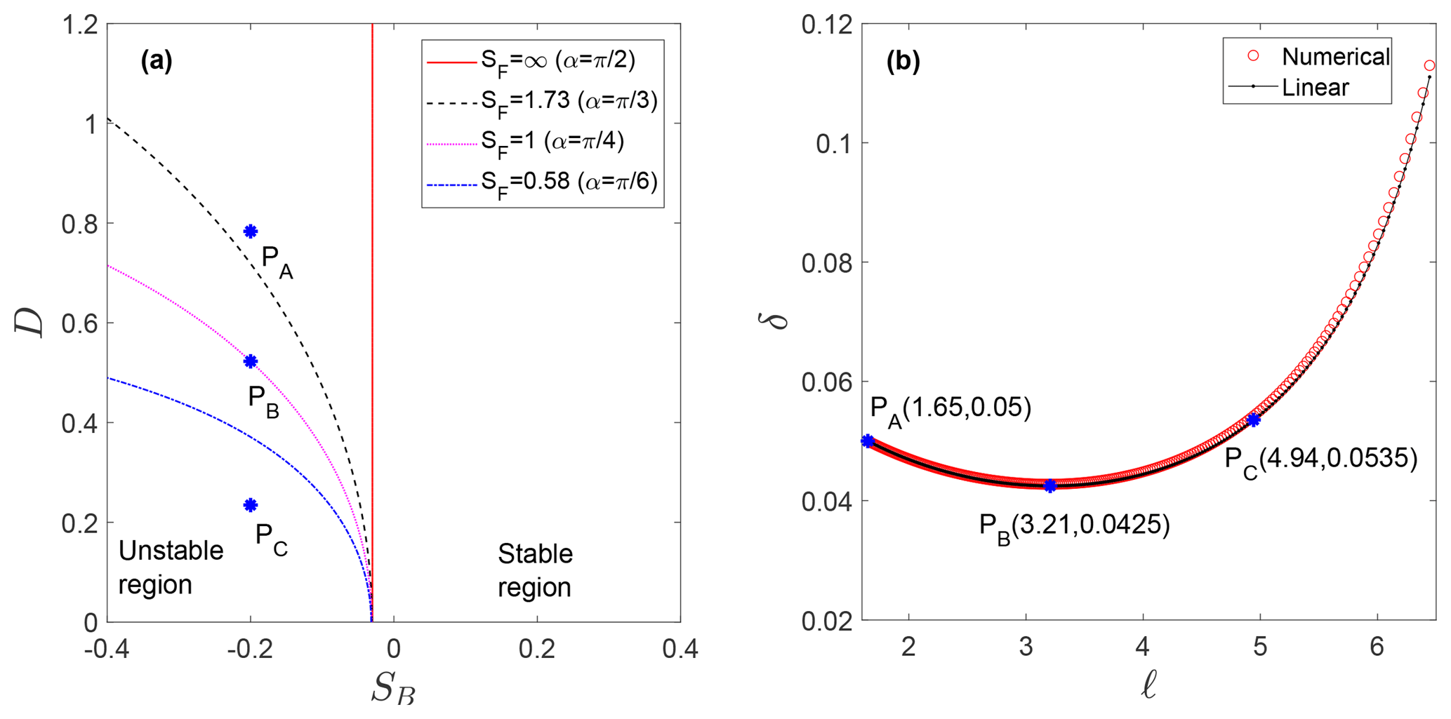
Figure 3 (a) The stability region of the absolute criterion for different foreset slopes S_F with k=1 and S_T=0.03. When S_F=1, the point P_A is in a stable region, the point P_B is on a boundary between the stable and unstable region, and point P_C is in an unstable region. (b) The amplitude of the shape perturbation δ as a function of bulk shoreline position ℓ, in the case where the initial t=0 shape of the shoreline is $x(t=\mathrm{0})=\mathrm{1.65}+\mathrm{0.05}\cos \left(y\right)$ and the foreset slope is S_F=1, and there is a linear variation ($\mathrm{0.95}-\mathrm{0.2}(x-\mathrm{1.6})$ m) of the water depth.

We can also use the above conditions to test the validity of the linear theory used in the derivation of the stability criterion; Eq. (13). In particular, following an approach used in previous works (Li and Li, 2011; Zhao et al., 2016), we have developed a semi-implicit boundary-element-like scheme to compute the nonlinear dynamics of a shoreline. In these nonlinear computations, we measure the growth of the perturbation as $\mathit{\delta }\left(t\right)=max\left|\right|\mathit{x}|-\mathrm{\ell }(t\left)\right|$, where x is the position vector of the shoreline. The linear prediction is in excellent agreement with our nonlinear results (see Fig. 3b). In particular we note that, in the nonlinear analysis, the minimum perturbation 0.0428 is reached at position ℓ=3.19 – values close to the linear analysis counterparts of 0.0425 and 3.21. Moreover, we have performed a series of simulations using different initial perturbations and confirmed that the difference between the linear and nonlinear results is indeed O(ϵ²).

4.2  Choice of characteristic length scale

Following the typical approach of a morphological instability analysis (see Sekerka et al., 2014), we can look for two characteristic wavelengths associated with our shoreline perturbations. The first of these is the wavelength associated with the fastest growing wave number; given sufficient time, we would expect this to be the dominant wavelength of the evolving instability. The second is the wavelength associated with the wave number at which the amplitude of the perturbation neither grows or decays – the neutral wavelength.

In the case of the initial perturbation exhibiting a number of modes ($x(y,t)=\mathrm{\ell }\left(t\right)+\mathit{ϵ}{\sum }_{k=\mathrm{1}}^{\mathrm{\infty }}{\mathit{\delta }}_k\left(t\right)\cos \left(ky\right)$), each mode independently evolves following Eq. (12). In this circumstance, we can determine, essentially by direct inspection of Eq. (12), that the fastest growing wavelength would be associated with the wave number k=0, corresponding to an infinitely long wavelength – recall that wavelength $\mathit{\lambda }=\frac{\mathrm{2}\mathit{\pi }}{k}$. This presents something of a conundrum: while an infinite wavelength is mathematically consistent with our analysis, it is unlikely to be physically achievable. Rather, we would expect that the dominant wavelength observed, in a given system, would be set by the lateral size of the system (e.g., the width of an experiment or the distance between channels).

Perhaps a better length scale to characterize the nature of unstable shoreline growth is the neutral wavelength. On appropriate rearrangement, this wavelength can be calculated by the substitution of the wave number definition $k=\frac{\mathrm{2}\mathit{\pi }}{{\mathit{\lambda }}_{\mathrm{n}}}$ into our stability criterion (Eq. 13):

$$\begin{array}{}\text{(16)}& {\mathit{\lambda }}_{\mathrm{n}}={\displaystyle \frac{\sqrt{\mathrm{2}}\mathit{\pi }D}{\sqrt{-S_{\mathrm{F}}{S}_{\mathrm{B}}^{\mathrm{e}}}}},-S_{\mathrm{B}}>\mathrm{0}.\end{array}$$

The value of λ_n provides us with a minimum lateral length scale for the resulting morphology of the growth of an unstable shoreline.

4.3 Values of neutral wavelength in experimental and field systems

Our contention is that, determining the possible values of the neutral wavelength in experimental and field systems will inform us regarding the expected length scales of the instability in delta shoreline growth along adverse basement slopes.

As an example, let us again consider the end-point conditions found in the XES10, Hajek et al. (2014) experiment. In this case, as the sediment toe advances onto the adverse slope, the neutral wavelength Eq. (16) linearly decreases from a value of λ_n(1.6)=11.41 m to a value of λ_n(5)=3.24 m at the maximum length of the experiment. Hence, the neutral wave length of the instability is close to or beyond the lateral length of the experiment, y=3 m (Hajek et al., 2014). Note that extending the length of the adverse slope to the point where the water depth D→0 would allow smaller wavelengths to become unstable. For example, at x=6.3 m (D=0.1 m), the neutrally stable wavelength is λ_n(6.3)=0.12 m . At this point, however, there is a very limited remaining longitudinal domain over which the instability can develop.

Figure 4 Atchafalaya 1935 bathymetry data. Panel (a) shows the location of three profiles of a length of ∼6 km; the profiles start ∼10 km offshore, are in a direction normal to the shoreline, and cover a lateral range of 3 km. Panel (b) provides the bed elevations along each of the profiles; the average slope of these profiles is taken as $S_{\mathrm{B}}=-\mathrm{0.00015}$.

As for the determining values of neutral wavelengths that could be characteristic of field settings, we consider predictions from Eq. (16) using data from two adverse slopes in natural settings. First, in recognition of the active delta building in the Wax Lake–Atchafalaya Bay area in the Gulf of Mexico (Wagner et al., 2017), we use the 1935 pre-growth bathymetry data (Atchafalaya Bay, https://www.ngdc.noaa.gov/mgg/bathymetry/estuarine/, last access: May 2019). We stress that our intention here is not to model the growth of specific deltas in this system but rather to use the pre-delta bathymetry data to provide constraints on the spacial extent and values of pre-existing basement slope regimes in a field setting. To this end, we have selected a sampling region (3 km lateral, 6 km longitudinal extent), 10 km offshore of the Atchafalaya outlet. Figure 4 shows the location of three longitudinal profiles that span this system. These profiles indicate that, on average, the sample region has a persistent adverse slope $S_{\mathrm{B}}=-\mathrm{0.00015}$ in the offshore direction, along which the water depth changes from approximately 1.8 to 0.9 m. If we assume that the foreset is S_F=0.0002 and set the top set slope as S_T=0.00007 (values consistent with the current-day slopes on Wax Lake delta; Shaw et al., 2016; Wagner et al., 2017), we see that, as a shoreline advances along this adverse slope, the predicted neutral wavelengths (Eq. 16) are relatively large, compared to the system size. Linearly decreasing with offshore distance, we obtain values ranging from λ_n≈ 142 to 71 km. The two deltas growing in the modern Atchafalaya Bay are around 10 km in diameter, smaller than the predicted neutral wavelength, so we are led to conclude that if these advancing deltas were to encounter an adverse slope, the indication of the resulting unstable growth would not be observable.

As a larger-scale field example, we consider the Torok formation in the Colville Basin, as reported by Houseknecht et al. (2001). This formation displays clinoforms prograding over an adverse basement slope associated with a foredeep. Based on the schematic cross section shown in Fig. 7b of Houseknecht et al. (2001), we can estimate the adverse basement slope over which the shelf margin prograded. Over a distance of roughly 200 km, we measure a steady decrease in the clinoform height from around 1900 to 710 m. Assuming that the clinoform heights correspond to basin depth, a minimum estimate of |S_B| is $\mathrm{6}\times {\mathrm{10}}^{-\mathrm{3}}$. This estimate is a minimum because it does not account for relative sea level rise, which would cause the basin depth to increase over time. We measure a foreset slope of roughly 0.03, which is consistent with typical values for continental slopes. While we do not have an estimate for S_T available, it is reasonable to assume that it is small relative to the basement slope we measured. Based on these values, we obtain an estimate for the neutral wavelength λ_n that ranges from 689 to 257 km, decreasing as the shelf margin progrades into shallower water. The cross section reported in Houseknecht et al. (2001) spans a distance of 450 km, so here we see that the estimated neutral wavelengths are on the order of the system size.

5 Conclusions

In this work we have used a geometric model and a linear stability analysis to investigate conditions under which the progradation of a planar sedimentary delta shoreline could become unstable, i.e., a condition where a perturbation of the shoreline will grow faster than the shoreline advance. Under the conditions of a constant unit discharge and a non-subsiding basement, we find the following.

• A geometric model provides a simple condition for determining the onset of auto-acceleration, the positive seaward acceleration of the shoreline. This model shows that a necessary condition of auto-acceleration is an adverse basement slope with an absolute value exceeding the value of the top set (fluvial) slope; the amount of excess required to trigger auto-acceleration increases as the absolute value of the ratio of basement to foreset slope increases.

• A linear stability analysis shows that, in an auto-acceleration condition, the growth of a delta shoreline prograding on a fixed adverse slope will become unstable; i.e., lateral perturbations on the shoreline, greater than a particular neutral wavelength, will grow faster than its bulk advance.

• The analysis indicates that the fastest (dominant) growth perturbation wavelengths are at the lateral size of the system under consideration.

• In experiment and field systems the neutral wavelength of the perturbations (the wavelength at which there is no growth or decay) is expected to be large, in excess of the widths of experimental systems and well beyond delimiting field length scales such as distributary channel spacings.

Thus, while we have clearly provided a positive answer to the question of this paper (“Can the growth of a deltaic shoreline be unstable?”), we can also conclude that observing clear signals of unstable growth in typical experimental and field delta systems would be unlikely. In other words, while delta building along an adverse basement slope is unstable, the resulting signal of the shoreline growth instability in the landscape will probably be “shredded” by other surface building processes, e.g., channel avulsions and alongshore transport.