the Creative Commons Attribution 4.0 License.
the Creative Commons Attribution 4.0 License.
 | 24 Jun 2019
Spatial and temporal patterns of sediment storage and erosion following a wildfire and extreme flood
Daniel J. Brogan
Peter A. Nelson
Lee H. MacDonald
Post-wildfire landscapes are highly susceptible to rapid geomorphic changes, and the resulting downstream effects, at both the hillslope and watershed scales due to increases in hillslope runoff and erosion. Numerous studies have documented these changes at the hillslope scale, but relatively few studies have documented larger-scale post-fire geomorphic changes over time. In this study we used five airborne laser scanning (ALS) datasets collected over 4 years to quantify erosion and deposition throughout the channel network in two ∼15 km2 watersheds, Skin Gulch and Hill Gulch, in northern Colorado after a wildfire followed by a large, long-duration flood 15 months later. The objectives were to (1) quantify the volumes, spatial patterns, and temporal changes over time of erosion and deposition over a nearly 4-year period, and (2) evaluate the extent to which these spatially and temporally explicit changes are correlated to precipitation metrics, burn severity, and morphologic variables. The volumetric changes were calculated from a differencing of DEMs for 50 m long segments of the channel network and associated valley bottoms. The results showed net sediment accumulation after the wildfire in the valley bottoms of both watersheds, with greater accumulations in the wider and flatter valley bottoms in the first 2 years after burning. In contrast, the mesoscale flood caused large amounts of erosion, with higher erosion in those areas with more post-fire deposition. Only minor changes occurred over the 2 years following the mesoscale flood. Volume changes for the different time periods were weakly but significantly correlated to, in order of decreasing correlation, contributing area, channel width, percent burned at high and/or moderate severity, channel slope, confinement ratio, maximum 30 min precipitation, and total precipitation. These results suggest that morphometric characteristics, when combined with burn severity and a specified storm, can indicate the relative likelihood and locations for post-fire erosion and deposition. This information can help assess downstream risks and prioritize areas for post-fire hillslope rehabilitation treatments.
- Article
(26057 KB) - Full-text XML
- BibTeX
- EndNote


Wildfires alter hydrologic response by creating conditions that can lead to greatly increased runoff and erosion rates. At plot to hillslope scales increased rates of runoff have been attributed to a decrease in canopy cover, ground cover, and surface roughness and an increase in soil sealing and soil water repellency (e.g., Benavides-Solorio and MacDonald, 2001; Huffman et al., 2001; Larsen and MacDonald, 2007; Onda et al., 2008; Larsen et al., 2009; Ebel et al., 2012; Stoof et al., 2012; Schmeer et al., 2018). At the hillslope scale these fire-induced changes increase a variety of erosional processes, including rainsplash, sheet flow, rilling, gullying, landslides, and debris flows (e.g., Benda and Dunne, 1997; Inbar et al., 1998; Cannon et al., 2001; Gabet and Dunne, 2003; Roering and Gerber, 2005; Wagenbrenner and Robichaud, 2014; Rengers et al., 2016b). As spatial scale increases channel erosion can become important (e.g., Meyer et al., 1992; Legleiter et al., 2003; Wagenbrenner and Robichaud, 2014), but at larger scales the predominant post-fire response is deposition, including alluvial fans, channel infilling, floodplain accretion, reservoir filling, and a sediment super slug (e.g., Moody and Martin, 2001; Reneau et al., 2007; Santi et al., 2008; Orem and Pelletier, 2015; Moody, 2017).
Considerable advances have been made in understanding post-wildfire runoff, erosion, and mass wasting at hillslope and small watershed scales (see Shakesby and Doerr, 2006; Moody et al., 2013, and references within); however, the larger-scale effects of fires on flooding, water quality, and sedimentation are often the most significant due to their adverse human and resource impacts (Hamilton et al., 1954; Doehring, 1968; Moody and Martin, 2001, 2004; Rhoades et al., 2011; Writer et al., 2014). Despite recent advances in modeling basin-scale post-wildfire runoff (Rengers et al., 2016a), most efforts to model post-fire runoff and erosion have focused at the hillslope scale, and include WEPP (e.g., Elliot, 2004; Miller et al., 2011), RUSLE (Renard et al., 1997), AGWA (Goodrich et al., 2005), and ERMiT (Robichaud et al., 2007). The first two models have been used as the basic building blocks for predicting changes at scales larger than a few hundred hectares (e.g., GeoWEPP; Miller et al., 2011; Elliot et al., 2016), but downstream post-fire flooding, erosion, and sedimentation are not a simple sum of hillslope-scale processes. Accurate predictions and upscaling from hillslopes require a more explicit consideration of sediment storage and erosion, and a failure to do so will result in unreliable estimates of watershed-scale peak flows, sediment production, sediment deposition, and sediment delivery (e.g., Moody and Kinner, 2006; Stoof et al., 2012). Efforts to measure and better understand larger-scale geomorphic changes have been hampered by the lack of high-spatial- and high-temporal-resolution data at the watershed scale (Moody et al., 2013). The lack of quantitative data has precluded a spatially explicit evaluation of the controls on the volumetric changes in erosion and deposition throughout a channel network (e.g., Pelletier and Orem, 2014; Orem and Pelletier, 2015).
To some extent the larger-scale effects of fires should be analogous to the observed patterns of erosion and deposition following large floods (e.g., Wolman and Eiler, 1958). More specifically, stream power – or gradients in stream power – and lateral confinement have typically been the best predictors of the spatial patterns of erosion and deposition (e.g., Miller, 1995; Fuller, 2008; Thompson and Croke, 2013; Gartner et al., 2015; Stoffel et al., 2016; Surian et al., 2016; Yochum et al., 2017), although strong correlations are not always apparent (e.g., Nardi and Rinaldi, 2015). Total energy expenditure during floods (Costa and O'Connor, 1995) can be equally important as stream power and lateral confinement in estimating total sediment transport (e.g., Wicherski et al., 2017). In contrast to fire studies, studies on the geomorphic impacts of extreme floods have usually focused on the erosional changes, even though short-duration, high-energy floods may cause substantial sediment deposition (e.g., Magilligan et al., 2015; Brogan et al., 2017).
New technologies, such as repeat airborne laser scanning (ALS), offer the potential to greatly improve our ability to quantify and analyze post-fire sediment storage and erosion over time and space (sensu Passalacqua et al., 2015). However, the decimeter-scale uncertainty in detecting elevation change means that ALS differencing is most useful in stream channels and valley bottoms where the elevation changes are more likely to exceed the measurement uncertainty.
In June 2012 the High Park Fire (HPF) burned 350 km2 of primarily montane forest just west of Fort Collins, Colorado, US. Within the HPF burn area we began intensively monitoring two similar ∼15 km2 watersheds to quantify post-wildfire geomorphic changes (viz., Brogan et al., 2019). Subsequent convective storms created a unique comparison between the two watersheds, as a high-intensity summer thunderstorm just 1 week after burning caused very extensive downstream deposition that was not replicated in the other watershed. A total of 15 months after burning, an exceptionally large and long-duration mesoscale flood caused sustained high flows and channel erosion in both watersheds, and this severely altered the expected post-fire trajectory of persistent and progressively declining deposition. We were fortunate to have two ALS datasets to evaluate the post-fire changes prior to the mesoscale flood and three more ALS datasets to document the flood and 2 more years of post-fire effects. This unique collection of sequential ALS data allows us to both quantify and compare the geomorphic changes due to the fire and the flood over time and space. We can also infer how the different amounts of deposition in the two watersheds may have altered the relative effects of the mesoscale flood. The validity and our understanding of the ALS differences were greatly enhanced by several closely related studies, including the intensive monitoring of 21 channel cross sections and longitudinal profiles in the two study watersheds (Brogan et al., 2019), estimated peak flows due to the large convective storm 1 week after the fire was contained (Brogan et al., 2017, 2019), the identification of precipitation thresholds for runoff and sediment delivery (Wilson et al., 2018), measured hillslope-scale erosion rates (Schmeer et al., 2018), and a more limited study of the hillslope erosion rates and channel changes in summer 2013 (Kampf et al., 2016). Together these data allow us to answer two key questions: (1) what are the spatial and temporal patterns of erosion and deposition following a wildfire and a large flood in the valley bottoms of small- to moderate-sized watersheds (0.1–15 km2) and (2) to what extent can these patterns be related to precipitation depths and intensities, burn severity, and valley and basin morphology? The results should help predict the likelihood and potential magnitude of downstream erosion and deposition after large high-severity wildfires and large floods, and hence the potential for adverse downstream effects.
Two proximate and very similar watersheds, Skin Gulch (SG) and Hill Gulch (HG), were selected to investigate post-wildfire geomorphic changes (Fig. 1). Both watersheds burned in the High Park Fire, both drain north into the Cache la Poudre River, and they are similar in size at 15.3 and 14.2 km2, respectively. In SG elevations range from 1890 to 2580 m, while HG is about 8 km to the east and therefore slightly lower at 1740 to 2380 m (Table 1). Average terrain slopes and drainage density for SG and HG are very similar at 23 % and 24 %, and 2.5 and 2.3 km km−2, respectively. The two watersheds have nearly identical hypsometric curves with much of the area at mid-elevations, although there are some flatter areas in the upper portions of each watershed. About 81 % of SG and 89 % of HG is largely unmanaged coniferous forest that is predominantly ponderosa pine with some increasing amounts of Douglas fir and lodgepole pine on north-facing slopes and at higher elevations (Jin et al., 2013). SG is predominantly National Forest land, while HG is primarily privately owned. In each watershed there are several very small reservoirs that were presumably established as stock ponds. A control watershed could not be identified due to the lack of sequential ALS data outside of the High Park Fire.
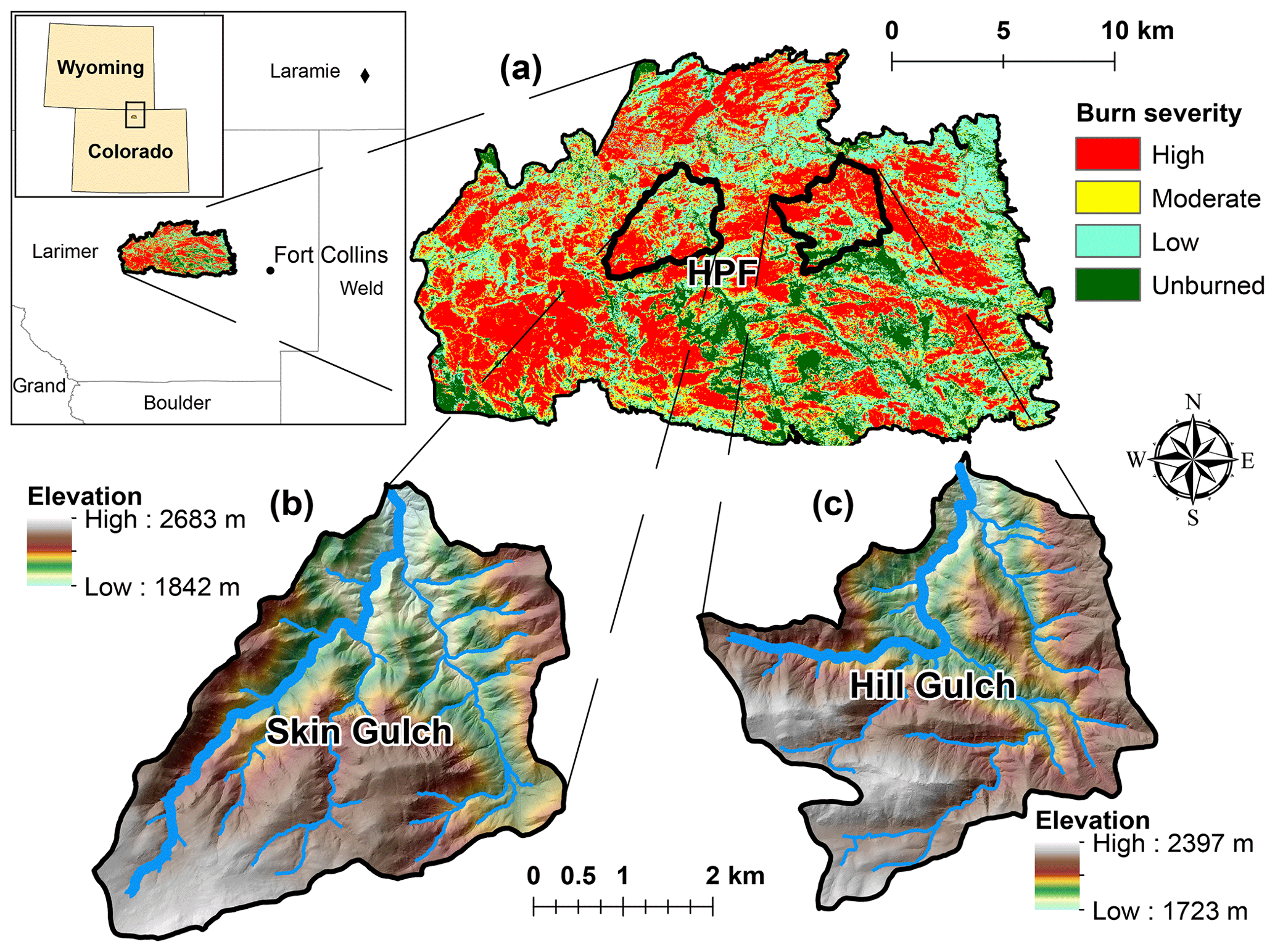
Figure 1Location and burn severity of the (a) High Park Fire (HPF) in the Colorado Front Range of the western US, and elevations of (b) Skin Gulch and (c) Hill Gulch. Inset map shows the city of Fort Collins and the surrounding counties, and the black diamond is the location of the KCYS Doppler radar station in Cheyenne, Wyoming. The thick blue lines in each watershed represent the reach used to present longitudinal results in Figs. 8 and 9.

Figure 2Seasonal changes in vegetation led to spurious deposition during fall to summer DoDs (a), and spurious erosion in the summer to fall DoDs (b). The valley bottom in (a) and (b) includes several woody deciduous species along with some ponderosa pine (c). Panel (d) shows the remaining change after using our raster-based algorithm to reduce the errors due to leaf out and leaf drop. Red circle in (c) identifies the upper half of a person standing in the understory, and the pink star in (d) represents the approximate location of the photo in (c).
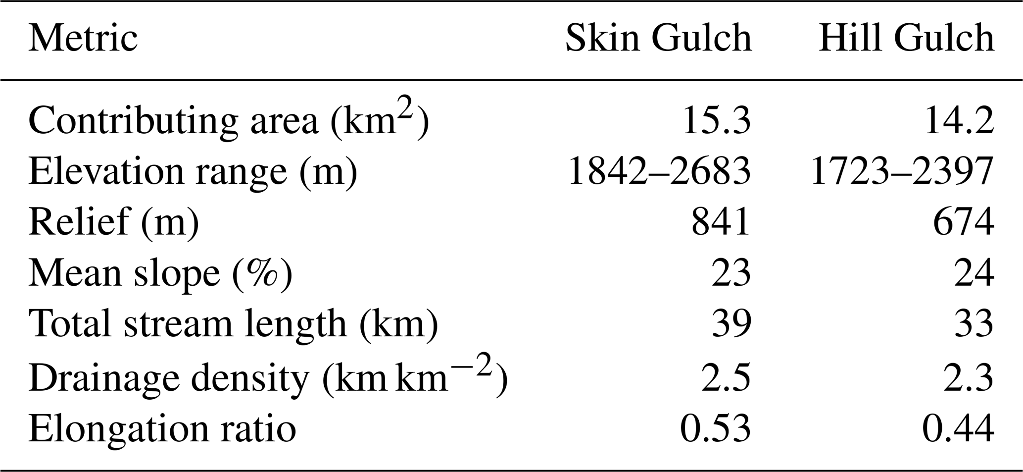
Table 1General watershed metrics for Skin Gulch and Hill Gulch.
Approximately 65 % of each watershed was burned at moderate to high severity. In SG most of the area burned at moderate to high severity was in the upper headwaters, while in HG most of the moderate- to high-severity burned areas were in the lower portion of the watershed (Fig. 1). Straw and wood mulch were applied from helicopters in 2012 and 2013 to approximately 6 % and 18 % of the hillslopes in SG and HG, respectively. The underlying geology is primarily schist with scattered rock outcrops (Abbott, 1970, 1976; Braddock et al., 1988), and the soils are predominantly Redfeather sandy loams (HPF BAER Report, 2012; Soil Survey Staff, 2018). Headwater reaches range from wide shallow swales to steep and confined channels; the middle reaches are generally steep and confined with scattered floodplain pockets; and the downstream reaches are wider with mostly continuous floodplains. Sediment is stored predominantly in the channel bed and on the floodplains. The area is characterized as semiarid with mean annual precipitation of 450–550 mm (PRISM Climate Group, Oregon State University, http://prism.oregonstate.edu, last access: 1 October 2018). Summer precipitation is usually derived from convective thunderstorms, while spring and fall storms tend to be lower-intensity frontal storms. Approximately one-third of the annual precipitation falls as snow.
Streamflow in both watersheds was seasonal prior to burning, and the downstream main stem channels were only about 1–2 m wide. After the fire streamflow noticeably increased and became perennial. About 1 week after the fire had been contained a convective storm in SG generated large amounts of hillslope and upstream channel erosion and extensive downstream deposition (Brogan et al., 2017). Two-dimensional hydraulic modeling yielded an estimated peak flow – without accounting for sediment bulking – of nearly 30 m3 s−1 km−2, and this event is henceforth referred to as the “convective flood”. There was no comparable storm in HG, but both watersheds were subjected to a series of smaller convective storms during each of the summers. The other major event was a spatially large and long-duration mesoscale storm in September 2013 that caused extensive destruction throughout the Colorado Front Range as well as widespread and prolonged high flows in both SG and HG. Peak flows were estimated to be 2.3–5.7 m3 s−1 km−2 in SG and 0.9–1.4 m3 s−1 km−2 in HG, with the range of values depending primarily on whether the peak flow was modeled with pre- or post-flood topography (Brogan et al., 2017, 2019).
3.1 ALS preparation
In each of the 4 years after the fire, an ALS dataset was collected over the entire burn area by the National Ecological Observatory Network (NEON) Airborne Observatory Platform. Each ALS dataset is referred to in this paper by the year and month of collection using the format of yyyymm, so the four NEON datasets are 201210, 201307, 201409, and 201506. A fifth ALS dataset, 201310, was collected by the U.S. Geological Survey (USGS) and Federal Emergency Management Agency (FEMA) in fall 2013 to help assess the damage caused by the September 2013 mesoscale flood. The four time periods between the five ALS datasets are referred to in this paper as T1, T2, T3 and T4. The 201307 ALS data in SG had substantial alignment issues, so we used OPALS (Orientation and Processing of Airborne Laser Scanning software; Mandlburger et al., 2009) to improve the flight line alignment. We attempted to estimate the volume changes in the channels and valley bottoms for the first summer after burning by constructing point clouds from 2008 aerial photographs using structure from motion (Filippelli, 2015). Unfortunately the extensive vegetation cover prevented the accurate delineation of bare-earth elevations over most of the study area, and this meant that we were not able to quantify the post-fire deposition that occurred prior to the first ALS dataset in October 2012.
For each ALS dataset the raw point clouds were merged, ground classified, and clipped to our two study watersheds using LAStools (Isenburg, 2015). Ground classification parameters included a buffer of 50 m, a step size of 5 m, and an extra fine search for initial ground points. From these processed point clouds we created digital elevation models (DEMs) with 1 m ×1 m pixels (Isenburg, 2015). Care was taken to align all ALS DEMs as closely as possible using a Python script to calculate the differences in slopes and aspects between each NEON DEM and the 201310 USGS/FEMA DEM (following Nuth and Kääb, 2011). The resulting estimate of the XYZ translation required to rectify the location of each NEON DEM was repeated until translation changes in X, Y, and Z were less than 1 cm, or the required shift for that iteration was less than 2 % of the overall required shift. Each point cloud was shifted by the computed translation, and DEM rasters were recreated from the translated point clouds. Finally, the rectified point clouds were compared to total station and real-time kinematic GNSS (RTK-GNSS) survey points to calculate the mean absolute error (MAE) as an indication of the accuracy of each ALS dataset.
3.2 Delineating and characterizing the valley bottoms and contributing areas
We used FluvialCorridor, an ArcGIS Toolbox that extracts a number of riverscape features (Roux et al., 2015), to delineate the valley bottoms in each watershed from the 201310 DEM. Defining a channel network is the first step, and for this we set a contributing area threshold of 0.1 km2 based on local field surveys (Henkle et al., 2011). The valley bottom was then computed and adjusted using a number of user-controlled input parameters, such as elevation threshold aggregation and disaggregation distances, buffer sizes, and smoothing tolerance. We adjusted these parameters until the valley bottom delineation satisfactorily matched aerial photographs and 2 m contour lines derived from the 201310 DEM.
Valley bottom polygons were segmented into 50 m long sections oriented in the downstream direction, yielding 595 segments in SG and 559 segments in HG. A segment length of 50 m was selected because this length is sufficiently long to characterize the local morphometrics while also allowing for a relatively high-resolution assessment of the rate of change in slopes, valley bottom widths, and other characteristics. The 50 m segments also match the typical length of the longitudinal profiles that we surveyed to obtain higher-temporal-resolution data on channel geomorphic changes (Brogan et al., 2019). FluvialCorridor did have difficulty characterizing valley bottoms for the headwaters of several tributaries with gently sloping topography; the resulting unrealistically wide valley bottoms caused us to remove 89 and 56 segments in the headwaters of SG and HG, respectively. Another eight segments near the outlet of SG were excluded because the deposited sediment was repeatedly excavated by the state highway department (for example see Fig. 10C in Kampf et al., 2016). Seven more segments in lower SG were excluded during T4 due to channel realignment and rehabilitation efforts, and one segment was excluded in lower HG during T4 due to the reconstruction of a house. A few other segments were removed from each watershed due to small reservoirs and unreliable ground classification. Ultimately 490 segments in SG and 484 segments in HG were used for summarizing morphometrics (see Sect. 3.4) and for statistical analysis (see Sect. 3.7), and these represent 83 % of the total channel length in SG and 87 % of the total channel length in HG.
Contributing area polygons were delineated for each segment using a looped Python script that uses the “Hydrology” toolset and “Raster to Polygon” tool in ArcGIS. The resulting polygons were used to determine the total precipitation and maximum 30 min precipitation intensities for each segment for each of the four time periods (see Sect. 3.3 for more detail). Percentage of area burned at both high severity (BSh) and moderate severity (BSm) was determined for the contributing area of each segment using the burn severity (BS) map derived from RapidEye imagery and a multistage decision tree (Stone, 2015).
3.3 Precipitation
The amount and intensity of precipitation over the two study watersheds was determined from the National Weather Service WSR-88D Doppler radar in Cheyenne, WY, corrected with local daily rain gage data. We began by converting the dual-polarized 1 h precipitation accumulation (DAA) radar products into gridded precipitation estimates using a 0.5 km grid. The precipitation was summed for each grid cell from 07:00 to 07:00 local time to match the daily rain gage data. These radar estimates were then compared to the rain gage estimates to come up with a daily mean field bias (Wright et al., 2014):
where Bi is the bias for day i, Gij is the daily precipitation for day i and gage j, and Rij is the summed 24 h precipitation for day i and radar pixel containing j. Sources of gage data include 4 in. diameter rain gages monitored by members of the Community Collaborative Rain, Hail & Snow (CoCoRaHS) Network (https://www.cocorahs.org/, last access: 31 July 2018), and tipping-bucket gages monitored by researchers at Colorado State University, the National Center for Atmospheric Research, and the U.S. Geological Survey. The number of rain gages used to compute the bias ranged from 36 to 97 depending on how many of the tipping-bucket gages were active and how many manual observations were recorded for a given day. These gages were located in and around our study watersheds, with the farthest gage being 40 km away.
Daily total precipitation and maximum 30 min precipitation intensity (MI30) were calculated from the bias-corrected DAA radar data for every 0.5 km grid cell across the HPF from October 2012 to November 2015. MI30 was chosen over other intensity intervals (e.g., MI5, MI15) because it correlates best with peak flood discharge (Moody et al., 2013), and is also closely correlated with peak stage (Kean et al., 2011) and with hillslope erosion rates from the HPF (Schmeer et al., 2018). Since volume changes over the intervals between ALS datasets represent cumulative geomorphologic effects, daily precipitation was summed for each of the four time periods. In contrast, the maximum MI30 value between each ALS dataset was determined for each cell in each watershed. Finally, the mean total precipitation and the maximum MI30 were computed for the upstream area of each channel segment for each DEM of difference (DoD). This meant that the maximum MI30 values for different cells within a given contributing area did not always originate from the same storm as the different summer thunderstorms were often very localized.
3.4 Topographic and hydraulic controls
A series of valley bottom, channel, and contributing area metrics, called morphometrics in this paper, were estimated for each 50 m segment. These data were correlated to the calculated volume changes to help determine possible controls on the volumes of erosion, deposition, and net change. A series of Python scripts were written to clip, extract, and compute morphometrics directly from the DEMs and/or a combination of outputs from FluvialCorridor (e.g., stream network, segment polygons, valley widths). Streamline networks for each ALS dataset were created for each watershed, and the mean channel slope (S) for each segment was determined by the slope of a linear regression on streamline elevations extracted from each ALS dataset at 1 m intervals. Topographic curvature (ΔS) was quantified for each segment by calculating the slope of the linear regression between the channel slopes of a given segment and the two upstream segments versus distance upstream. A positive slope indicates an increasing slope and negative curvature, while a negative slope indicates a decreasing slope and a positive curvature. Valley width (wv) was computed at 1 m intervals along the valley centerline and an average width was calculated for each 50 m segment. Valley constriction and expansion (Δwv) was computed in the same way as ΔS. Since the resolutions of the DEMs and aerial imagery were too coarse to accurately delineate the channels, channel width (wc) was estimated from a regional downstream hydraulic geometry equation (Bieger et al., 2015):
where A is the drainage area in square kilometers and channel width is in meters.
We defined channel confinement (Cr) as the ratio of valley width to channel width. Unit stream power, a hydraulic control, is often a good predictor of erosion and deposition (e.g., Baker and Costa, 1987). Unit stream power (ω) is equal to
where γ is the specific weight of water (N m−3), Q is discharge (m3 s−1), and Sf is the friction slope (m m−1). Because continuous stage or flow data were not available, and given the potential uncertainty in the regression equation for wc, we used the ratio of channel slope to valley width as a proxy for stream power. Downstream changes in the slope ∕ width ratio were computed in the same way as ΔS and Δwv.
3.5 Valley change
DEMs of difference (DoDs) were computed using the geomorphic change detection (GCD) tool add-in for ArcGIS (http://gcd.riverscapes.xyz/ (last access: 1 September 2018), version 6; Wheaton et al., 2010). GCD uses a fuzzy inference system (FIS) to propagate spatially explicit DEM uncertainties, and consequently the uncertainties in the DoD. Spatially explicit errors are much more accurate than assuming a uniform uncertainty, as the latter can lead to large errors in the calculated volumes of erosion and deposition (e.g., Wheaton et al., 2010; Milan et al., 2011).
Point quality, point density, and slope were included as membership functions in our FIS procedure. We assumed uniform point quality based on the accuracy of the ALS after adjustment (i.e., the MAE for each dataset). Point density was computed for each DEM pixel based on the point cloud, and slopes were derived directly from the DEM. After differencing the DEMs, pixels with elevation changes smaller than the spatially propagated errors were ignored, and the remaining values constitute the thresholded DoD. The GCD tool also calculates total volumes of erosion, deposition, and net change, along with the uncertainty for each volume estimate. The uncertainties in the total volumes of erosion and deposition were computed by multiplying individual error heights by the pixel area and summing these. Uncertainty in each net volume difference was propagated from the corresponding uncertainties in erosion and deposition. Using the thresholded DoDs and our own Python script we computed the volumes of erosion, deposition, and net change for each 50 m segment for each time period.
The sign and overall magnitude of ALS-derived volumetric changes for the 50 m segments were compared to the measured changes for the 10 cross sections in SG and 11 cross sections in HG (Brogan et al., 2019). The measured changes in cross-sectional area were multiplied by 50 m to obtain volumes that were then compared to the calculated ALS volume changes for the 21 channel segments where there was a cross section.
3.6 Removal of spurious vegetation artifacts
A visual check of the DoD results revealed the calculated volume changes were being affected by seasonal changes in leaf cover. For example, some locations had up to 3 m of deposition calculated from fall to summer (i.e., 201210–201307, or T1, 201409–201506 or T4), and nearly identical amounts of erosion from summer to fall (i.e., 201307–201310, or T2). Vegetation issues were not immediately obvious in the 201310–201409 or T3 DoD, as both ALS datasets were collected in the fall. A raster-based algorithm was written to identify possible spurious changes due to changes in the deciduous leaf cover on a pixel-by-pixel basis for the DoDs that covered different seasons (i.e., T1, T2, and T4). An example of the algorithm's logic is as follows: If for a given pixel the change in both fall-to-summer differences (T1 and T4) were small, but the change from summer-to-fall (T2) was large compared to the T1 and T4 changes, it would indicate that vegetation was contaminating the signal at that location. This logic applies for other combinations of DoD differences, and takes the form of Algorithm 1.
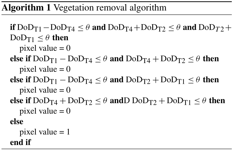
In Algorithm 1, DoDT# refers to the DoD for a given time period (i.e., T1, T2, or T4), and θ is a threshold in meters. We used this algorithm to classify each pixel as a 0 or 1, with 0 indicating a seasonal vegetation artifact when at least two of the three DoDs showed a difference in elevation change that was less than or equal to 1 m (θ). This raster of 1's and 0's was multiplied on a cell-by-cell basis for each DEM to exclude those pixels with a seasonal vegetation artifact for that DoD, and the GCD tool was rerun to more accurately estimate the volume and uncertainty of geomorphic changes. Figure 2 shows an example of this vegetation filtering for a location in Skin Gulch that showed around 1–3 m of deposition from fall 2012 to summer 2013 (Fig. 2a) and around 1–3 m of erosion from summer 2013 to fall 2013 before filtering out the seasonal artifacts (Fig. 2b). A site visit in September 2016 verified the lack of such large vertical geomorphic change and confirmed a predominantly deciduous cover of narrowleaf cottonwood, Rocky Mountain maple, alders, chokecherry, and wild raspberries (Fig. 2c).
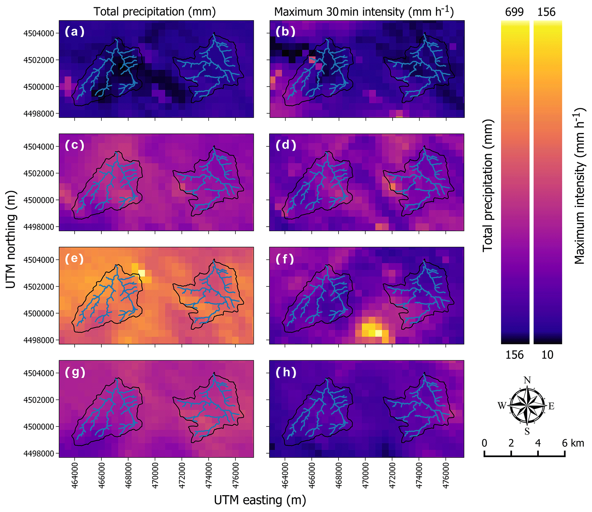
Figure 3Total precipitation (mm) and maximum 30 min intensity (mm h−1) for each of the four time periods for (a, b) T1 (201210 to 201307), (c, d) T2 (201307 to 201310), (e, f) T3 (201310 to 201409), and (g, h) T4 (201409 to 201506). Within each panel Skin Gulch is the watershed on the left and Hill Gulch is to the right.
3.7 Statistical analysis of controls on erosion and deposition
Pearson correlation coefficients (r) were calculated between the different site factors and the erosion, deposition, and net volume changes in the 50 m segments for each of the four time periods and each watershed. The different site factors were total precipitation, MI30, percent of contributing area burned at high and/or moderate severity, and drainage network morphometrics as explained in Sect. 3.4. Since some of the morphometric variables changed from the beginning to the end of a given time period (i.e., S, ΔS, , and ), we calculated the correlations for each time period using both the beginning and end values. We found negligible differences in the strength of the correlations depending on whether we used the beginning or end values, so we only present the results for the values at the beginning of each time period. Normalizing the net volume changes by contributing area generally did not improve the correlations, so these results are also not presented here. Correlations were also calculated after stratifying the data by channel slope (< or ≥4 %) and contributing area (< or ≥4 km2), but these results are not presented as these did not greatly improve the correlations or lead to clear insights about the underlying processes. We did not stratify the data by physiographic unit or lateral confinement as suggested by Rinaldi et al. (2013) and Nardi and Rinaldi (2015) because the stream types in our two study watersheds were predominantly cascade channels (Montgomery and Buffington, 1997). It should be noted that a positive correlation indicates increasing deposition or decreasing erosion with an increasing independent variable, while a negative correlation indicates decreasing deposition or increasing erosion. We recognize that each stream segment is not necessarily spatially independent because upstream erosion or deposition can affect downstream segments or reaches, but autocorrelations of the dependent variables generally fell below r=0.5 for five segments upstream or downstream. This correlation analysis provides a useful, initial assessment of how morphologic and site characteristics are generally related to the magnitudes of erosion, deposition, and net volumetric change. In the results we primarily focus on correlation coefficients that are either greater than 0.32 or less than −0.32 (i.e., r2>0.10).
Precipitation
Total precipitation and maximum 30 min intensities varied considerably between each DoD time period, but the values were relatively similar within and between the two watersheds (Fig. 3). Total precipitation was lowest during T1 with a mean in SG of only 174 and 185 mm in HG (Table 2 and Fig. 3a). The T1 period also generally had the lowest MI30 values other than a few very localized high-intensity storms (Table 2 and Fig. 3b). Mean total precipitation over the short second period was much larger than in T1 with 366 mm in SG and 327 mm in HG (Table 2), with most of this rainfall due to the mesoscale storm. Total precipitation was relatively evenly distributed over the two watersheds (Kampf et al., 2016). Precipitation intensities during the mesoscale flood generally did not exceed 40 mm h−1 (Kampf et al., 2016), but intense localized thunderstorms prior to the mesoscale flood generated some of the highest MI30 values recorded over the period covered by the ALS datasets (Table 2 and Fig. 3d).
Table 2Mean total precipitation and mean maximum 30 min intensities (MI30) for Skin Gulch and Hill Gulch for each time period. Ranges are in parentheses, and the values are derived from the gage-corrected radar data.
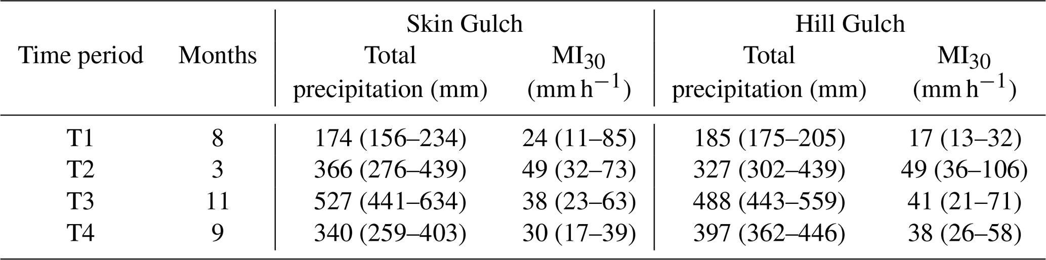
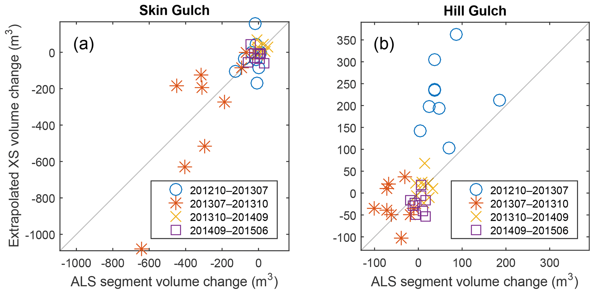
Figure 4Plots of the extrapolated cross section (XS) volume changes versus the corresponding ALS segment volume changes for (a) Skin Gulch and (b) Hill Gulch. Diagonal lines are the 1:1 relationship, and the different symbols in each plot represent the different time periods.
The third period was nearly a year so it had relatively high total precipitation values but low MI30 values (Table 2 and Fig. 3f). As in T1 and T2, the relative variation in maximum MI30 values was much greater than the variation in total precipitation due to the high spatial variability of the summer thunderstorms. Mean total precipitation in T4 was lower than in T3 (Table 2), and the mean MI30 values of around 30 mm h−1for SG and 38 mm h−1 for HG (Fig. 3h) were both lower than in T2 and T3, indicating less potential for hillslope erosion and downstream channel change.
4.1 ALS data accuracy and valley morphometrics
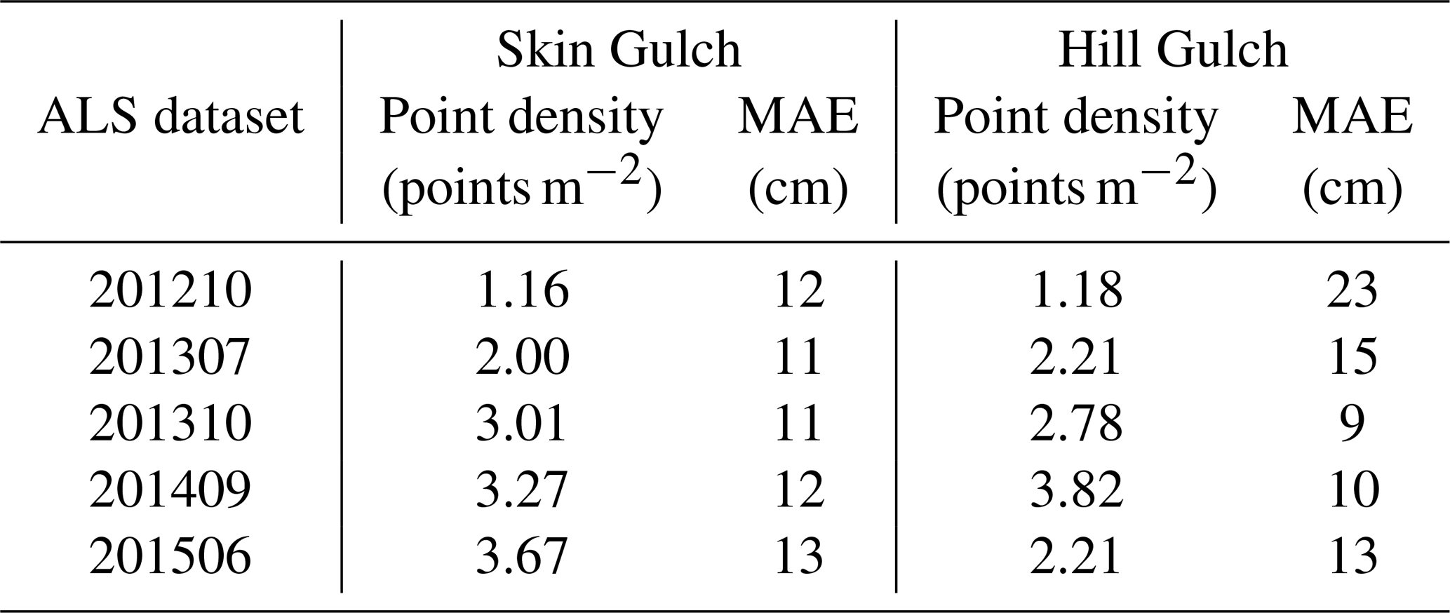
Point density increased with each ALS dataset from a minimum of just under 1.2 points m−2 in the first ALS dataset to over 3.5 points m−2 for the last dataset in Skin Gulch and the next to last dataset in Hill Gulch (Table 3). After alignment the mean absolute errors (MAEs) of the ALS point clouds were only 9–13 cm except for the first and second ALS datasets in HG, which had MAEs of 23 and 15 cm, respectively (Table 3).
Table 3Point density and average mean absolute error (MAE) for each ALS dataset for Skin Gulch and Hill Gulch, respectively. MAE was determined by the elevation difference between total station and RTK-GNSS survey points and interpolated ALS points.
The volume changes estimated from cross section data and the calculated volume changes from the ALS data for the corresponding segments generally plot close to the 1:1 line except for the first time period in Hill Gulch and one cross section in the second period in Skin Gulch (Fig. 4). Some differences between these two datasets should be expected given that the measured cross-section change was extrapolated to the entire 50 m segment. The key point is that the ALS differencing results appear to be valid given the general agreement in the sign and magnitude of the ALS differencing and measured cross-section changes.
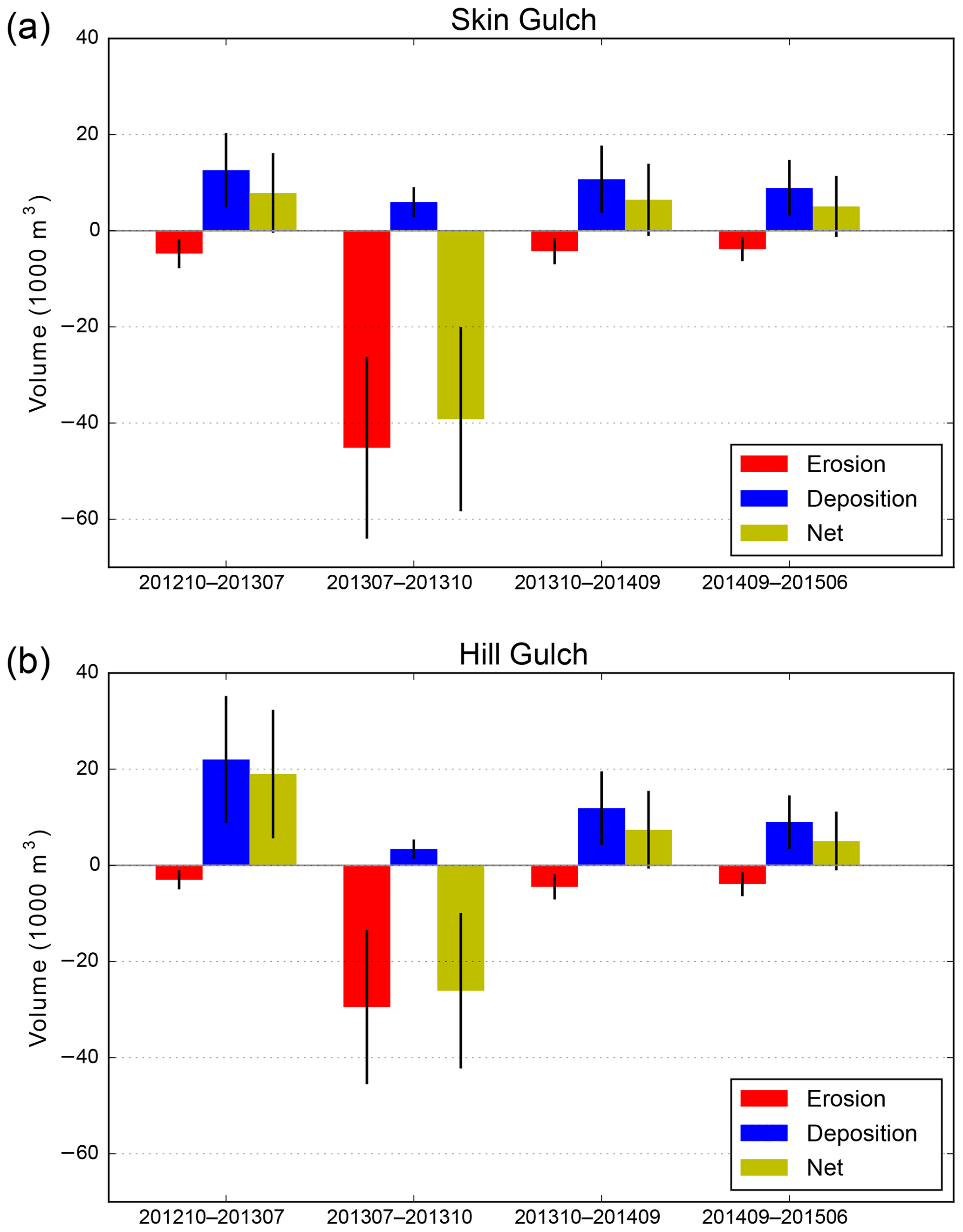
Figure 5Total valley erosion, deposition, and net volume change for each time period for (a) Skin Gulch and (b) Hill Gulch. Black vertical bars indicate the uncertainty for each volume estimate.
The overall comparability of SG and HG is further confirmed by the generally similar spatial distributions and trends in channel slopes, valley widths, and confinement ratios. For the 490 segments in SG and 484 segments in HG used in our analyses 86 % and 73 % had channel slopes greater than 0.065 m m−1, respectively, and were classified as cascade according to Montgomery and Buffington (1997). A total of 13 % of the channel segments in SG and 22 % of the segments in HG had channel slopes of 0.03 to 0.065 m m−1, which would be classified as step pool. Less than 2 % of the segments in SG and 5 % of the segments in HG had channel slopes less than 0.03 m m−1. The few channel segments with slopes less than 0.03 m m−1 are primarily in a few headwater areas, near tributaries, and towards the outlet of each watershed.
Valley widths tended to increase downstream, with the exception of certain headwater locations where FluvialCorridor had difficulty characterizing the valley bottoms. Approximately 80 % of the valley widths in each watershed were between 10 and 40 m. As might be expected, confinement ratios tended to decrease downstream and were relatively similar in the two watersheds with about 75 % of the valley bottoms having values between 10 % and 35 %, about 20 % having values greater than 35, and no segments having a confinement ratio below 5.
4.2 Spatial and temporal erosion and deposition volumes
The T1 period (201210–201307) only began after the first summer of thunderstorm-driven runoff and erosion, so the two main periods of geomorphic change were spring snowmelt and the first summer thunderstorms. Snowmelt runoff was almost entirely erosional while the summer thunderstorms were primarily depositional but highly variable in space, and these different processes are reflected in the high variability and complex spatial patterns of deposition and erosion within and between the two watersheds (Figs. 5–9; see also Figs. A1–A4). Many of the headwater reaches in SG had little or no erosion or deposition, while in the middle portions of SG there was more extensive deposition (Fig. 6a), particularly along the main stem about 4–5 km above the outlet (Fig. 8b). Lower in the watershed there were areas with substantial amounts of net erosion with some deposition, particularly in the eastern tributary (Figs. 6a and 8b). The total net volume change was nearly 8000 m3 of deposition (Fig. 5a), but our extensive field observations indicate that the total post-fire deposition was actually much larger as the first lidar data were collected only after the summer thunderstorms. It is of interest that the greatest erosion of 130 m3 in one 50 m segment was just downstream of a confluence about 2 km above the outlet (Fig. 8b), which is where our field observations showed tremendous sediment deposition from the exceptionally large convective rainstorm and flood that occurred just 1 week after the fire (see reference to confluence and XS6 in Brogan et al., 2017, 2019). This confluence marks a very large decrease in channel slope for the west branch of Skin Gulch and a tremendous widening of the valley bottom (Fig. 8a), which largely explains the large amount of deposition. In HG there was much more net deposition during T1, and the calculated volume of 19 000 m3 was spread throughout much of the channel network (Figs. 5b, 7a, and 9b). Much of this deposition was in the middle reaches where the channel slopes decreased to less than ∼0.10 and valley widths increased to more than ∼30 m (Fig. 9). Similar to SG, a number of the headwater reaches had only minor erosion or deposition (Fig. 7a). Aerial imagery and soil data (Soil Survey Staff, 2018) indicate that these areas are steep with a high density of exposed rock outcrops, suggesting a limited capacity for both channel incision and deposition.
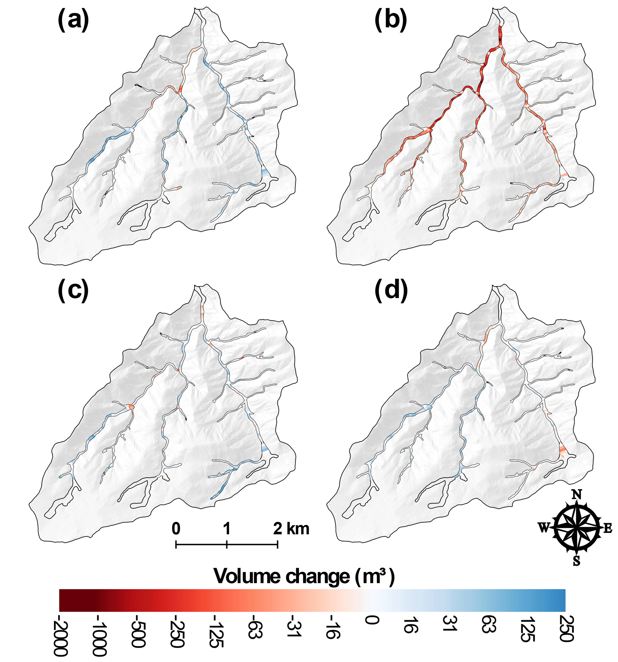
Figure 6Net volume differences for each valley bottom segment in Skin Gulch for (a) T1 (201210–201307), (b) T2 (201307–201310), (c) T3 (201310–201409), and (d) T4 (201409–201506). Calculated volumes are not reported for the transparent segments in the headwaters and segments furthest downstream (outlined by heavier black lines) due to unrealistically wide valley widths, repeat excavations, or the ground surface not being reliably determined.
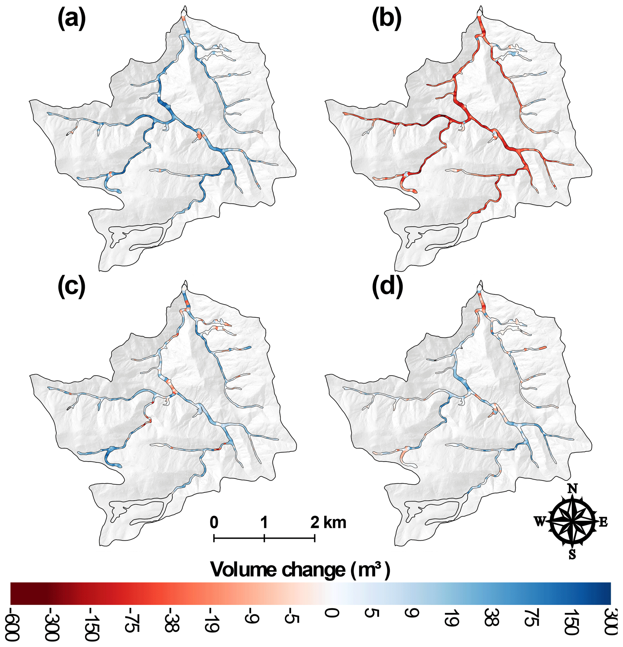
Figure 7Net volume differences for each valley bottom segment in Hill Gulch for (a) T1 (201210–201307), (b) T2 (201307–201310), (c) T3 (201310–201409), and (d) T4 (201409–201506). Calculated volumes are not reported for the transparent segments in the headwaters and segments furthest downstream (outlined by heavier black lines) due to unrealistically wide valley widths, repeat excavations, or the ground surface not being reliably determined.
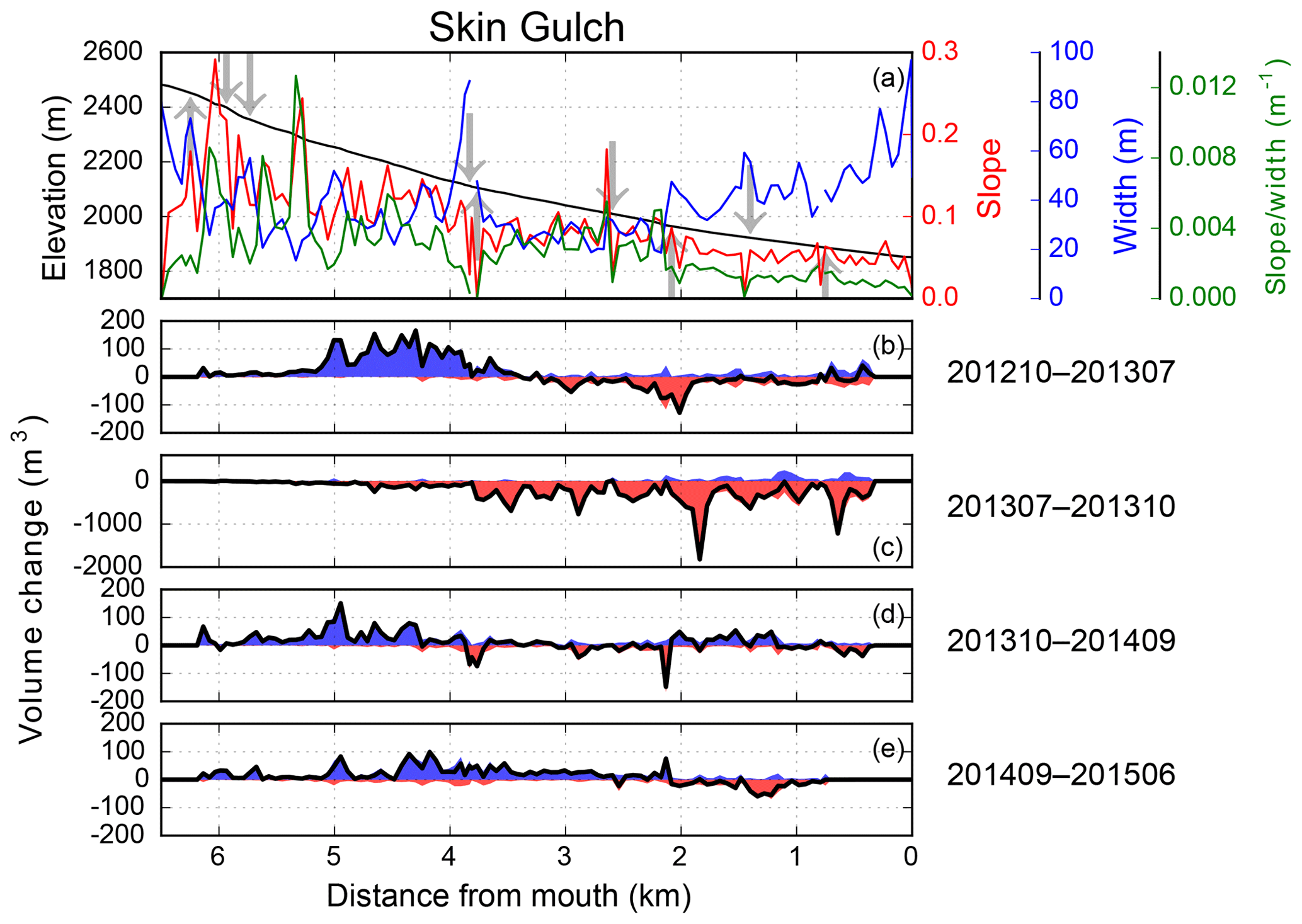
Figure 8Longitudinal distributions in Skin Gulch of (a) elevation, channel slope, valley width and slope ∕ width, and the corresponding longitudinal changes in volumes for (b) T1 (201210–201307), (c) T2 (201307–201310), (d) T3 (201310–201409), and (e) T4 (201409–201506). Up and down arrows in (a) represent tributaries that enter the main channel from the right and left, respectively. Blue and red areas in (b)–(e) are deposition and erosion, respectively, and the black line is net volume change. Removal of excess sediment and restoration activities means that the data for the lowest 400 m were excluded for all time periods, and for the lowest 700 m in (e). See Fig. 1 for the location of the reaches being represented, and the data in (a) were taken from the 201310 lidar dataset.
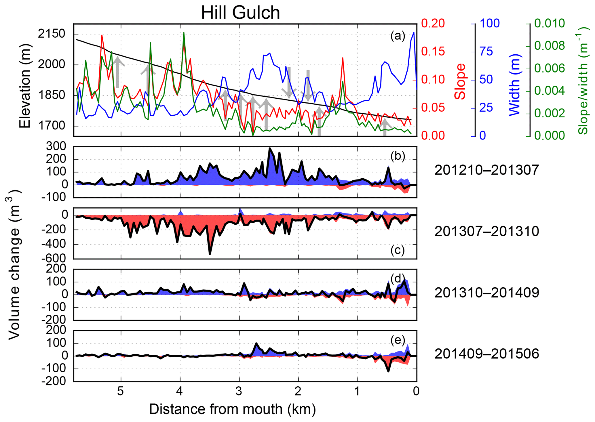
Figure 9Longitudinal distributions in Hill Gulch of (a) elevation, channel slope, valley width and flood power, and the corresponding longitudinal changes in volume for (b) T1 (201210–201307), (c) T2 (201307–201310), (d) T3 (201310–201409), and (e) T4 (201409–201506). Up and down arrows in (a) represent tributaries that enter the main channel from the right and left, respectively. Blue and red areas in (b)–(e) are deposition and erosion, respectively, and the black line is net volume change. See Fig. 1 for the location of the reaches being represented, and the data in (a) were taken from the 201310 lidar dataset.
In September 2013 the mesoscale flood caused widespread and often dramatic erosion in SG (Brogan et al., 2017, 2019). While there was some deposition in the downstream channels due to the summer thunderstorms (Brogan et al., 2019) (Fig. 8c), the total net change in SG was 39 000 m3 of erosion, with the vast majority of this occurring in the middle and downstream reaches (Figs. 6b and 8c). In the middle portion of the watershed channel incision was particularly prevalent in the narrower valley bottoms (see Figs. 4.13D, 4.13E, and 4.13F in Brogan, 2018). Often the segments with the greatest eroded volumes were where we had observed larger amounts of deposited sediment from summer 2012 that could be easily eroded. From a more process-based perspective, the sediment available for erosion consisted of pre-fire deposits accumulated over centuries to millennia (Cotrufo et al., 2016) that would have been somewhat protected from erosion by the vegetative cover, while the post-fire sediment was more readily accessible because it usually was at lower elevations within the valley bottom and unprotected by any vegetative cover. Overall the total erosion in SG during T2 was 3.6 times larger than the total deposition during T1, and this large discrepancy can be largely attributed to the fact that most of the post-fire sediment had been deposited in summer 2012 prior to the first ALS survey (Brogan et al., 2017, 2019).
HG also experienced widespread erosion during T2 (Figs. 5b and 7b; Brogan et al., 2017, 2019), but the net volume change was only two-thirds of the value calculated for SG (Fig. 5). Some of the greatest erosion occurred where there was more pre-fire sediment storage, including floodplain pockets (e.g., ∼2.4, ∼3.7, and ∼4.7 km), tributary junctions (e.g., ∼2.2 and ∼3.3 km), and colluvial deposits from hollows (e.g., ∼4.4 km; Fig. 9). Substantial erosion also occurred where the hillsides constricted the valley width to less than 20 m; for example, there was over 800 and 1300 m3 of erosion around 3.4–3.5 and 3.8–4.0 km from the outlet (Fig. 9c). The pattern of erosion during T2 closely mirrored the depositional patterns from T1 (Figs. 8 and 9), and this was particularly true for HG because there was qualitatively less deposition in summer 2012 prior to the first lidar dataset and proportionally more deposition during T1. For example, during T1 there was an estimated 2300 m3 of deposition in the valley bottom between 2 and 3 km upstream of the outlet, and this large amount of deposition was associated with a slope decrease to around 0.04 m m−1 and an increase in valley width to 55 m. During T2 this same reach experienced 2700 m3 of erosion, or just slightly more than the amount of deposition during T1.
During T3 the patterns of erosion, deposition, and net change in both watersheds were similar in direction and location to T1 but smaller in magnitude (Fig. 5), with the decline in magnitude attributed to the reduced upslope erosion due to vegetative regrowth (Schmeer et al., 2018). SG and HG had more similar magnitudes of change in T3 than in T1 because there were no undocumented periods of erosion or deposition. In SG there again was substantial deposition about 4–5 km upstream of the outlet (Fig. 8d), while going downstream there was a more even balance between erosion and deposition (Fig. 6c). In HG there tended to be more consistent deposition from the headwaters to the outlet than in SG (Fig. 7). The total volumes of erosion and deposition were slightly greater in HG than in SG, but this difference was much smaller than the 2–3-fold difference in T1 (Fig. 5). The largest volumes of sediment deposition were in the headwaters and the lowest portion of the watershed where the sediment left by the mesoscale flood could be reworked and transported by spring snowmelt and the runoff from summer thunderstorms (Fig. 7c).
The T4 period had smaller volume changes than any of the other time periods (Fig. 5). Like T1 and T3, the overall pattern was deposition with net volume increase of just over 5000 m3 in both SG and HG. Most of the net erosion was focused in the lowest portions of the watersheds, especially in lower HG where there had been more deposition in T3 and therefore more sediment to be eroded in T4 (Figs. 6d, 7d, 8e, and 9e). The similarities between the two watersheds in the amounts and patterns of erosion, deposition, and net volume changes indicate a similarity in the primary driving processes of summer thunderstorms, hillslope erosion, downstream deposition, and erosion due to snowmelt. The lower absolute magnitude of these changes in T4 is consistent with the overall trend of vegetative recovery leading to less runoff and erosion as observed in other fires in the Colorado Front Range (e.g., Benavides-Solorio and MacDonald, 2005).
To summarize, the calculated volume changes for SG and HG were similar in their direction over the four time periods, and they also generally had roughly similar trends in magnitude (Fig. 5). There was a positive net volume change in T1, T3, and T4 for both watersheds, and other studies have documented that the primary effect of the High Park Fire and the summer thunderstorms was erosion at the hillslope scale (Schmeer et al., 2018) and deposition in the lower portions of both SG and HG (Brogan et al., 2019). The data presented here show that this post-fire deposition occurred nearly throughout the entire channel network, and that amount of geomorphic change decreased sharply over time, particularly in HG where the estimated net volume change dropped from nearly 20 000 m3 in T1 to just over 7000 and 5000 m3 in T3 and T4, respectively (Fig. 5b). In SG the net volumes over these same time periods also decreased from nearly 8000 m3 in T1 to over 6000 m3 and then 5000 m3 in T3 and T4, respectively (Fig. 5a). This overall pattern of deposition was counterbalanced by the large volumes of erosion during T2 as a result of the mesoscale flood. Hence in SG the total deposition over the four time periods was just over 38 000 m3, while the total erosion was nearly 50 % larger because the mesoscale flood eroded virtually all of the sediment that had been deposited in summer 2012 but was not captured by the first lidar dataset. In HG the total deposition over all four time periods was just over 46 000 m3, and this was very similar to the total erosion over the study period of nearly 41 000 m3. The importance of the mesoscale flood is indicated by the fact that 78 % of the total erosion in SG and 72 % of the total erosion in HG took place during T2. This means that, in the absence of the highly unusual mesoscale flood, the HPF would ultimately have caused extensive net deposition throughout nearly all of the channel network.
4.3 Statistical analysis of controls on erosion and deposition
Pearson correlation coefficients indicate that several of the independent variables were closely correlated with one or more of the other independent variables (Fig. 10; see also Tables A1 and A2). The strongest correlations between the independent variables included percentage of area burned at high severity and percentage of area burned at moderate and high severity (r=0.99 for both watersheds), slope ∕ width ratio vs. channel width ( in SG and in HG), and contributing area versus channel width (r=0.94 in SG and r=0.96 in HG). These relationships led us to remove percentage of area burned at high severity, slope ∕ width ratio, and channel width from further analyses. The removal of these three independent variables also necessitated the removal of the change in slope ∕ width ratio and the change in confinement ratio as these were also based on one of the independent variables that was removed from the analysis.
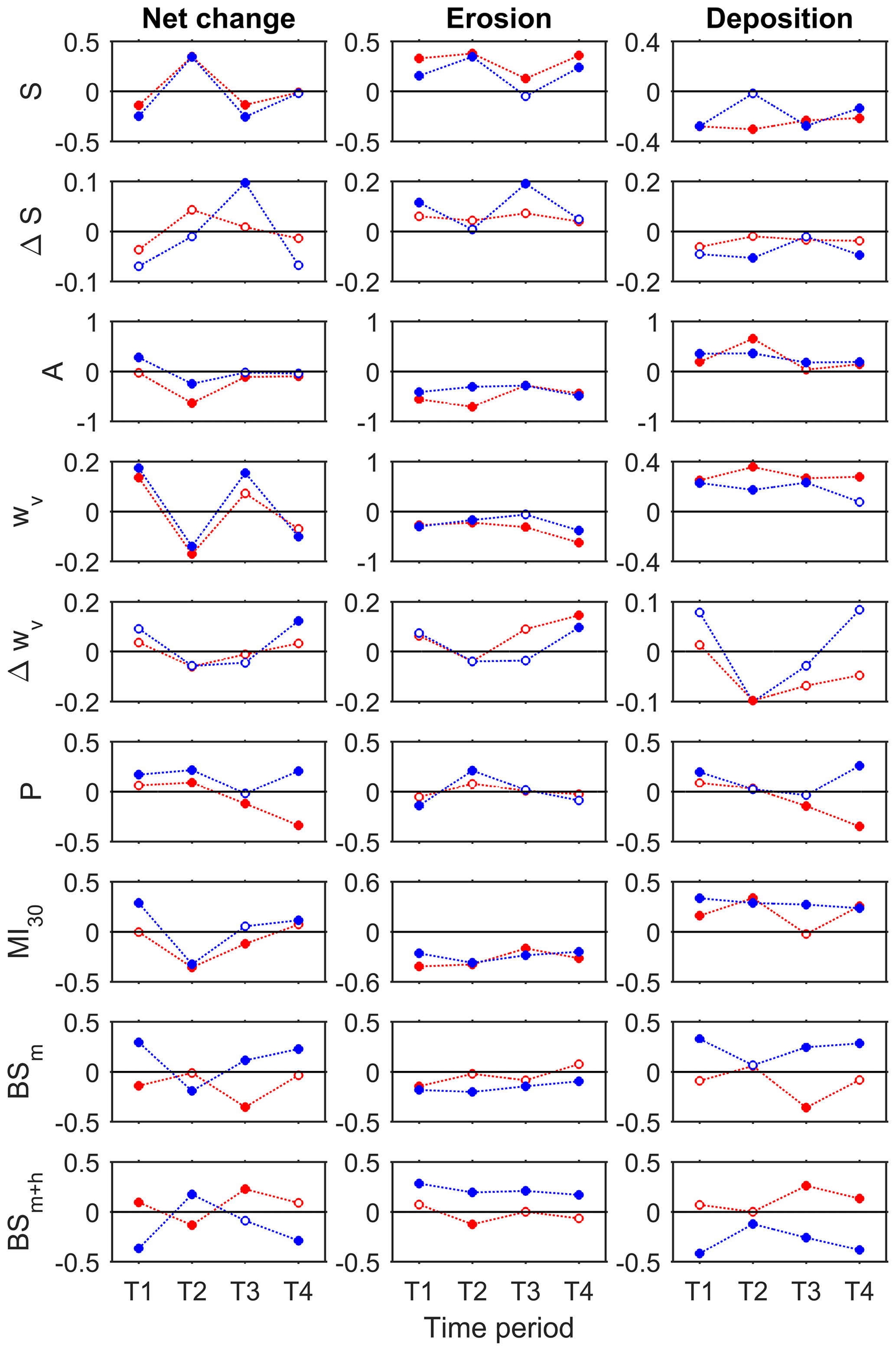
Figure 10Pearson correlation coefficients for Skin Gulch (dotted red lines) and Hill Gulch (dotted blue lines) for each time period between the independent metrics and the dependent variables of net volume change, total erosion, and total deposition, respectively. T1 to T4 are for the time periods (T#) of 201210–201307, 201307–201310, 201310–201409, and 201409–201506, respectively. Independent variables include channel slope (S), change in channel slope ΔS, contributing area (A), valley width (wv), change in valley width (Δwv), total precipitation (P), maximum 30 min intensity (MI30), percent burned at moderate severity (BSm), and percent burned at moderate and high severity (BSm+h). Filled circles indicate correlations that are significant at p value ≤ 0.05. Note that the vertical axes vary according to the strength of the correlations.
There was considerable variability in the correlation coefficients (r) between the various independent variables and the net volume change in each segment, and in the value of the correlations and across the four time periods (Fig. 10). Given the differences in the direction and magnitudes of geomorphic changes among the different time periods, the following sections summarize the key results for each successive time period, and we report correlations rather than coefficients of determination in order to indicate both the direction and the magnitude of the different relationships. By definition a positive correlation indicates that an increase in the independent variable is associated with either a decrease in erosion or an increase in deposition, while a negative correlation indicates that an increase in the independent variable is associated with either an increase in erosion or a decrease in deposition.
In SG the absolute correlations () for net volume change during T1 never exceeded 0.17 (Fig. 10), and this was primarily a result of the generally limited geomorphic change detected between the first and second ALS datasets (Figs. 6a and 8b). Since the T1 period did not capture the large amounts of deposition that were qualitatively observed in SG in the first 3 months after burning, the correlations were substantially stronger for segment-scale erosion volumes because the primary causal process was spring snowmelt rather than thunderstorm-driven deposition (Fig. 10). The independent variables that were most strongly correlated with segment-scale erosion volumes were contributing area (), MI30 () and channel slope (r=0.33). These results indicate that more erosion occurred in the lower gradient, wider downstream reaches with larger contributing areas, and this is because these reaches were where we qualitatively observed the greatest amounts of post-fire deposition and they therefore had more sediment that could be readily eroded by snowmelt and lower-intensity rainstorms. We posit that the correlations for deposition and net volume change in SG would have been much greater had the T1 period recorded the extensive post-fire deposition that was so apparent in the first summer after burning (Brogan et al., 2017, 2019).
Overall the correlations for T1 were slightly stronger in HG than in SG (Fig. 10). In contrast to SG, deposition in HG was more strongly correlated with the independent variables than either net volume change or total erosion. This difference is likely due to the greater magnitudes of deposition in the middle and lower reaches in HG relative to SG (Fig. 7). As in SG, two of the independent variables that were most strongly correlated with the volume of deposition were contributing area (r=0.35) and MI30 (r=0.34), and these are consistent with our understanding of the underlying causal processes of post-fire erosion and downstream deposition.
Further investigation of the scatterplots indicate that – particularly in SG – deposition predominated when contributing areas were less than about 4–5 km2, while erosion tended to dominate when contributing areas greater than about 4–5 km2. Since the T1 period only included spring snowmelt and smaller convective storms in the first part of summer 2013, this indicates that the smaller convective thunderstorms had limited impact at larger scales, while elevated baseflow could cause significant channel changes if there was sufficient readily erodible sediment in the channels and valley bottoms.
Correlations for T2 were generally stronger than for any of the other three time periods in both SG and HG, and this was primarily due to the substantial and consistent erosion resulting from the large mesoscale flood (Fig. 10; Brogan et al., 2017, 2019). In SG three metrics had r values >0.32 or with net volume change, and again these were contributing area (), MI30 (), and channel slope (r=0.35). These results indicate increasing erosion in the downstream direction and that nearly 40 % of the variance in the amount of net change can be explained solely by the increase in contributing area. The correlations with erosion were generally stronger than the correlations with net volume change, and the r value of −0.71 between contributing area and erosion for T2 in SG was the strongest correlation for any variable for any time period (Fig. 10). The correlations for HG were not as high as for SG, and this can be largely attributed to the lower volume changes in HG compared to SG (Fig. 5). In HG the two variables most strongly correlated with net volume change were again channel slope (r=0.35) and MI30 (). As in SG, correlations were generally stronger when the volume of erosion was the dependent variable compared to deposition (Fig. 10).
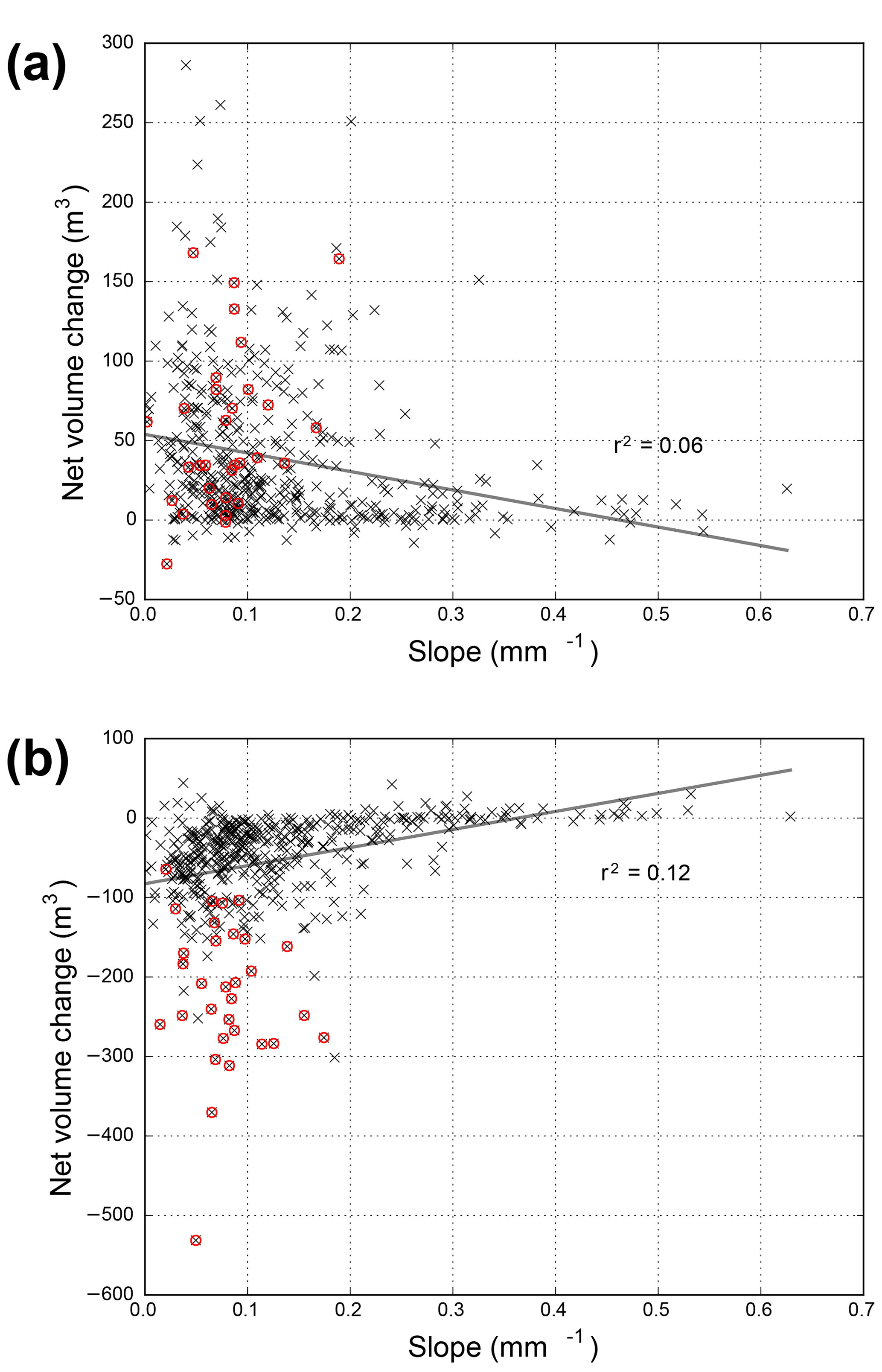
Overall the volume changes in T2 were similar in magnitude but opposite in sign to the volume changes in T1 (Figs. 8 and 9). Scatterplots of the segment-scale net volume changes for T2 against the net volume changes for T1 show that the bulk of the data plot along a line with a slope of −1 for SG and −0.8 for HG (Fig. 11). This indicates that the volumes eroded primarily by the mesoscale flood tended to be similar or proportional to the volumes deposited in T1. However, in both watersheds there are about 30 segments of the several hundred segments that had far more erosion in T2 than was deposited in T1; these points plot well below the regression line and are shown in red in Fig. 11a, d. In the case of SG these segments are almost exclusively along the channels where we observed massive deposition by the July 2012 convective storm along with some additional deposition by subsequent summer thunderstorms (Fig. 11c) (Brogan et al., 2017). Since this deposition was prior to the first ALS dataset, it should not be surprising that these points had much more erosion in T2 than deposition in T1. The sign changes in the correlations from negative to positive, or vice versa, between T1 and T2 are particularly notable for channel slope ( in T1 and 0.35 in T2) and valley width (r=0.13 in T1 and −0.17 in T2; Fig. 10), and these are consistent with the expected controls on post-fire deposition and flood-induced erosion, respectively.

Figure 11Regression of the net volume change for each 50 m segment for T2 (the period including the large erosional mesoscale flood of 201307–201310) against the net volume change for T1 (the depositional period of 201210–201307) for (a) Skin Gulch and (d) Hill Gulch. The red x's in (a) and (d) are the segments with much more erosion in T2 than deposition in T1, causing them to deviate substantially from the dashed line. The regression line and statistics for all of the data are shown in black, while the regression line and statistics in blue are for the truncated data after removing the red data points. (b) and (e) are burn severity maps of Skin Gulch and Hill Gulch, respectively, and the black boxes show the valley bottom segments in (c) and (f). The red segments in (c) and (f) are the red data points in (a) and (d).
In HG the volumes of deposition in T1 and erosion in T2 were more closely matched (Fig. 9) as indicated by the stronger r2 value of 0.40, but there is again a cluster of about 30 points below the line (Fig. 11d). The number and absolute magnitude of the differences between these points and the line is smaller than in SG, and this can be attributed to the smaller amounts of qualitatively observed deposition during the first summer after burning and the measured deposition during the T1 period, and hence the smaller volumes of sediment readily available for erosion by the mesoscale flood. A closer evaluation of the points below the line show that they come almost exclusively from a major tributary draining an area burned at high severity (Fig. 11e, f), and our field observations indicate that this area was subjected to extensive deposition prior to the first ALS dataset (see Fig. 3.9 in Brogan, 2018). If the points in red are excluded from the regression, the r2 increases to 0.64, and this confirms the relative importance of the initial post-fire storms in providing large amounts of sediment that were then eroded by the mesoscale flood. As in SG, many of the correlations between the independent variables and the volume changes shifted from negative to positive, or vice versa, between T1 and T2, including channel slope ( in T1 and 0.35 in T2), contributing area (r=0.28 in T1 and −0.24 in T2), and MI30 (r=0.29 in T1 and −0.33 in T2; Fig. 10).
In T3 and T4 the correlations between the independent variables and the segment-scale volume changes were generally low in both watersheds (Fig. 10). The lower correlations can be attributed in part to the much lower amounts of erosion and deposition (Fig. 5). The correlations in T3 and T4 generally had the same direction as in T1 because each of these periods was primarily depositional. In SG the only correlations with r>0.32 or (i.e., r2>0.10) were between net volume change and the percentage of area burned at moderate severity () in T3 and the total precipitation () in T4 (Fig. 10). In HG none of the independent variables explained much more than 8 % of the variation in net volume change, and the volumes of erosion and deposition were also only weakly correlated with the independent variables. In HG there were only three correlations with an r>0.32 or , and these were for increasing segment-scale erosion in T4 with increasing contributing area () and valley width () and decreasing deposition in T3 with increasing percentage of area burned at moderate and high severity (). The results for both watersheds indicate that the spring high flows continued to erode the relatively raw and enlarged channel created by the mesoscale flood.
5.1 Mechanisms of watershed-scale post-fire erosion, deposition, and recovery
When post-fire rainfall intensities exceed the sharply diminished infiltration rates (e.g., Cammeraat, 2004; Kampf et al., 2016), hillslope runoff is greatly enhanced and this causes a dramatic expansion and incision of the headwater channels (Wohl, 2013). The increased hillslope-channel connectivity and increased runoff transports the eroded sediment down into the channel network (e.g., Prosser and Williams, 1998; Schmeer et al., 2018), with the finer particles being readily transported much further downstream as suspended load. In contrast, the coarser sands and gravel are usually transported much shorter distances as bed load (e.g., Moody and Martin, 2001; Reneau et al., 2007), and are usually deposited in the wider, lower gradient reaches (e.g., Doehring, 1968; Anderson, 1976; Meyer et al., 1995; Moody and Martin, 2009).
The ash and sediment transported into the Cache la Poudre River after the High Park Fire greatly increased turbidities and suspended sediment concentrations (Writer et al., 2014), but our observations indicated that these sediment inputs generally did not alter the channel morphology of the main stem other than at a few tributary confluences, immediately behind a diversion dam, and much further downstream where the river suddenly emerges from the foothills into an unconfined valley bottom. Our qualitative observations indicate that fine sands, silts, and clays did not comprise much of the post-fire deposits in either the valley bottom of our two study watersheds or the main stem of the Cache la Poudre River. Particle-size data collected in both watersheds before the mesoscale flood show that only five of our 21 cross sections had a D16 smaller than 2 mm, and this dropped to only one cross section after the flood (Brogan et al., 2019). This means that the volume changes in our two study watersheds as quantified by the ALS differencing are primarily the deposition and subsequent movement of the coarser bed load particles.
Our study was unique in terms of being able to compare five ALS datasets taken over a 3-year period following the June 2012 High Park Fire and then the September 2013 mesoscale flood. These allowed us to quantify erosion and deposition volumes throughout the channels and valley bottoms in our two study watersheds on a spatially explicit basis. More specifically, we could calculate the combined effects of snowmelt and thunderstorms in the second summer after burning, evaluate the changes due to the mesoscale flood, and then quantify the changing volumes of erosion and deposition over the next nearly 2 years as the watersheds recovered from the fire and the flood. The resulting maps of valley bottom changes allow a far more detailed assessment of the spatial and temporal complexity of geomorphic changes than would be possible from manual measurements (sensu Schumm, 1973). While the ALS data do not allow us to fully separate the effects of snowmelt runoff versus summer thunderstorms, the results clearly show net deposition in both study watersheds during three of the four time periods, with net erosion in the second time period. This illustrates that – other than the mesoscale flood – the predominant post-fire effect is deposition in the downstream channels and valley bottoms (Fig. 5; see also Fig. 3.21 in Brogan, 2018), and that deposition from the summer thunderstorms substantially exceeds the erosion from snowmelt and low-intensity rainstorms. This preponderance of deposition over erosion is a typical post-fire response (e.g., Swanson, 1981; Morris and Moses, 1987; Moody and Martin, 2001; Wagenbrenner et al., 2006). Our more intensive field surveys of the cross sections and longitudinal profiles in each watershed do provide a more detailed assessment of post-fire changes within the larger time periods delineated by the ALS datasets (Brogan et al., 2019), but our field measurements necessarily represent only a relatively small fraction of the channel network. In contrast, the DoD results cover the entire channel network, but the trade-off is that the ALS differencing has a lower temporal resolution and higher measurement uncertainties due to alignment issues, horizontal displacement errors, interpolation errors, and errors due to leaf on and leaf off. Hence both types of data are needed to more accurately and completely characterize the effects of the High Park Fire and subsequent mesoscale flood, and together they highlight the importance of collecting data using different techniques at different spatial and temporal scales with their accompanying differences in spatial extent, temporal resolution, and measurement accuracy.
The smaller geomorphic changes in T3 and T4 relative to T1 are due to several factors. Of primary importance is the ongoing hillslope vegetation recovery, reduction in headwater channel length (Wohl and Scott, 2017), and relative paucity of large convective storms. Together these factors have resulted in a sharp decline in hillslope runoff, erosion, and connectivity as documented in the High Park Fire and other Front Range fires (Benavides-Solorio and MacDonald, 2005; Wagenbrenner et al., 2006; Schmeer et al., 2018), and these declines directly cause much smaller amounts of downstream deposition. In this study we also have to add another factor, which is the stripping and coarsening of the channel and valley bottoms due to the mesoscale flood (Brogan et al., 2019). The resulting reduction in available sediment in the channels and valley bottoms, when combined with the coarsening of the bed material in the active channel, limits the amount of erosion that can take place as a result of increased baseflows, runoff from convective thunderstorms, and spring snowmelt (e.g., Brunsden and Thornes, 1979; Thomas, 2001; Phillips and Van Dyke, 2016; Rathburn et al., 2017; Fryirs, 2017; Brogan et al., 2019). We should believe that the difference in the amount of deposition and net change between T1 and T3 and T4 is much larger than what we have shown here (e.g., Fig. 5) primarily because the first ALS data were collected after the first summer when there were very large amounts of post-fire sediment deposited in the channels and valley bottoms of both watersheds (Brogan et al., 2019), and also because of the poorer accuracy of the first ALS dataset.
The uncertainty in our ALS differencing also affects the extent to which we can fully understand the underlying geomorphic processes during our study. With average uncertainties of 10–15 cm, we generally could only detect elevation changes at tributary junctions and in larger channels and valley bottoms rather than on the hillslopes or in the headwater channels. Hence it was difficult to tell exactly where the break was between upslope incision versus downstream deposition. Most of the largest volume changes were in downstream locations where channel slopes were generally less than ∼10 % and valley widths were greater than ∼30 m. The limited accuracy of the ALS differencing also leads us to posit that we underestimated deposition more than erosion because deposition tended to be more widespread and shallower compared to the more localized and concentrated erosion.
5.2 Uncertainty, errors, and methodological issues in DEM differencing
It should be self-evident that future studies need to minimize the errors associated with DEM differencing if one is to accurately detect and quantify geomorphic changes, particularly in smaller streams. The challenges we encountered in working with five different ALS datasets suggests a set of best practices for using repeat ALS data to document geomorphic change after wildfires or other disturbances. First, ALS data collection must happen as soon as possible following the disturbance, particularly after fires as these landscapes are extremely sensitive to runoff, erosion, and channel change from even relatively small rainstorms (e.g., Shakesby and Doerr, 2006; Moody et al., 2013). Second, high-resolution topography should be repeated at the temporal resolution needed to distinguish and understand the seasonal effects of different driving forces (e.g., summer thunderstorms versus snowmelt). Recent advances in the use of drones and drone-based structure-from-motion (SfM) photogrammetry rather than airplanes should greatly facilitate more frequent lidar data collection (e.g., Tulldahl and Larsson, 2014), and allow data to be collected at a sufficiently high temporal resolution to capture the effects of discrete storms and floods rather than the combined effects that were inherent in our datasets. Drones can also provide data of substantially higher spatial resolution (e.g., Smith et al., 2016).
Third, repeat high-resolution topographic data often require translational rectification to better match the different datasets. In this study both vertical and horizontal translation was needed to more accurately match up the different ALS datasets, and thereby more accurately calculate elevation changes and associated volumes. Manual adjustments are laborious and non-repeatable, and our work was greatly facilitated by an automated approach to co-register the different point clouds (Nuth and Kääb, 2011). This approach, along with the availability of highly accurate RTK-GNSS field data (Brogan et al., 2019), reduced the vertical uncertainties of most of our ALS data to 10–15 cm. Fourth, ALS data should be collected at low altitudes with narrow flight pass widths, low scan angles, and good ground controls to improve the quality and density of the raw point clouds. The highest mean point density in our ALS datasets was 3.8 points m−2. We therefore recommend future studies aim for a minimum point density of 4 points m−2, as higher point densities would allow for a more detailed and accurate analysis.
Fifth, automated GIS tools now allow faster and easier characterization of the channel, adjacent topography, and specific geomorphic features; examples include FluvialCorridor (e.g., Roux et al., 2015), River Bathymetry Toolkit (e.g., McKean et al., 2009), TerEx (Stout and Belmont, 2014), V-BET (Gilbert et al., 2016), and the Valley Confinement Algorithm (Nagel et al., 2014). However, users must be aware of the limitations of these tools. FluvialCorridor provides objective valley bottom delineations that can be used over large spatial domains and it facilitates longitudinal segmentation of the channel and valley bottom, but we experienced problems in identifying valley margins when they were near very steep slopes. In some cases the delineated valley bottom included this adjacent steep slope or rock outcrop. In these locations ALS interpolation errors and horizontal displacement errors (Hodgson and Bresnahan, 2004) can lead to errors in estimating ground locations and elevations, resulting in substantial errors in the DoD volume estimates (e.g., Heritage et al., 2009; Wheaton et al., 2010; Milan et al., 2011; Bangen et al., 2016). These inaccuracies in identifying valley margins also caused higher elevation points to be included within a given segment, which will lead to inaccurate estimates of valley bottom slopes. Users of these automated tools need to carefully check the validity of any automated process, and we found it necessary to sometimes manually delineate the valley bottoms, especially when the valley bottoms were directly abutted by steep terrain.
Sixth, we tried to directly compute elevation differences from the point clouds (e.g., Lague et al., 2013), but procedures to do so are still in their infancy (Passalacqua et al., 2015). In our case we ended up using the standard DoD approach to compute the volumes of erosion and deposition because this resulted in lower uncertainties given our lower density point clouds (Hartzell et al., 2015). With raster-based differencing there is also a mature suite of tools to calculate spatially varying uncertainties, and this improves the accuracy of volume change estimates compared to assuming a uniform uncertainty (e.g., Wheaton et al., 2010; Milan et al., 2011).
Lastly, we had large errors due to the varying seasonal timing of the ALS datasets (i.e., leaf on versus leaf off). We therefore had to develop an algorithm to remove unrealistically large elevation changes due to changes in canopy cover. This procedure removed about 2 % of the valley bottom area from the analysis and this reduced the mean calculated total erosion, total deposition, and net volume differences by 46 % (s.d. = 16 %), 54 % (s.d. = 15 %), and 22 % (s.d. = 33 %), respectively. Conversely, the use of this algorithm increased the net volume change in T3 by 11 % in SG and 25 % in HG as it reduced total deposition more than total erosion. Careful manual checks of the DoDs and aerial imagery showed that this algorithm was still not able to always identify pixels with erroneous elevation changes due to changes in the vegetation heights between ALS datasets (e.g., Fig. 2d). Hence we strongly recommend that repeat ALS data be collected at similar times of the year, preferably during leaf off, to optimize the accuracy of the bare-earth DEMs and hence the accuracy and sensitivity for detecting elevation and volume changes. Our experience again shows that visual checks of DoDs are essential to detect various errors that otherwise would be presumed to represent real geomorphic change (e.g., Lane et al., 2004).
5.3 Controls on spatial and temporal patterns of geomorphic change
The linear regression results showed that post-fire volume changes for the different periods and watersheds were significantly correlated with precipitation depth and maximum 30 min intensities, percentage of area burned at moderate and/or high severity, and valley and basin morphology (Fig. 10). None of the independent variables had consistently strong coefficients of determination (r2) with segment-scale volume changes over the different time periods and watersheds, but the strongest relationships were generally with channel slope, contributing area, maximum 30 min precipitation intensity, and percentage of area burned at moderate and/or high severity. Precipitation intensity and burn severity both make physical sense as these are two of the dominant controls on the amount of sediment that is likely to be generated after a wildfire (e.g., Benavides-Solorio and MacDonald, 2005; Abrahams et al., 2018), while channel slope is a key control on both erosion and deposition. Contributing area will be directly related with the volume of runoff for both snowmelt and widespread storms like in September 2013, and segments with larger contributing areas also will tend to have larger channels and valley bottoms where larger volumes of sediment can be either deposited or eroded. Surprisingly, the volumes of erosion, deposition, and net change were generally not correlated with valley width, and this could be partially due to the issues with accurately delineating the valley bottoms.
We hypothesized that stronger correlations might be present when the watershed data were stratified by valley bottom slope or drainage area, but this did not greatly improve the strength of the correlations. It has been suggested that better relationships between volume changes and morphometric characteristics could be attained by parsing the valley into more discrete geomorphic units (e.g., channel, floodplain, terrace) to reflect different dominant processes (e.g., Weber and Pasternack, 2017), but there was no easy way for us to accurately identify these different geomorphic units throughout our study watersheds. The correlation results do help identify the key controls on the direction and magnitude of volumetric changes for the different time periods. Not surprisingly, the largest amount of deposition occurred in the first period after burning, while the mesoscale flood caused by far the greatest erosion. Correlations in the two periods after the mesoscale flood were lower due to both the lower magnitudes of erosion and deposition as the watersheds recovered from the fire and also the reduced sensitivity to channel change following the removal of post-fire sediment and the channel coarsening caused by the mesoscale flood. Overall the results here and from our field data (Brogan et al., 2019) strongly indicate that the magnitude of erosion in the channels and valley bottoms was largely controlled by sediment availability, and the closely related studies show that post-fire sediment availability is largely dependent on the combination of burn severity and the intensity of the summer thunderstorms (Kampf et al., 2016; Schmeer et al., 2018).
The importance of sediment availability is strongly supported by the observation that the volumes eroded in T2 were often very similar to the segment-scale volumes deposited in T1, with the discrepancies stemming mostly from the locations where there were large amounts of unrecorded deposition during the first summer after burning (Fig. 11; Brogan et al., 2017, 2019). There also was little net volume change in segments with a slope much greater than about 0.2 m m−1 (Fig. 12). In these steep channels the bed is comprised primarily of large, generally immobile clasts (e.g., Yager et al., 2012), and the steep slope means that there is very limited potential for storing the gravel and finer particles that comprise most of the post-fire sediment eroded by surface runoff. This means that efforts to predict potential geomorphic change may need to focus on quantifying where and how much sediment is available (e.g., Carling and Beven, 1989) rather than the spatial distribution of hydraulic and morphometric controls.
Areas of erosion and deposition are often highly correlated with the downstream gradient in stream power (e.g., Gartner et al., 2015; Yochum et al., 2017), but to our surprise none of our gradient metrics (i.e., ΔS, Δwv, ) were strongly correlated to net volume change, total erosion, or total deposition. Most of the largest volume changes occurred in segments where these gradients were close to zero, resulting in low correlation coefficients. These results again suggest that for our montane watersheds the spatial and temporal differences in sediment supply can better predict the volumes of erosion, deposition, and net change than local changes in slope or valley width.
Overall our correlations generally were not improved if erosion or deposition were used as the dependent variable instead of net volume change, but in some cases there were sharp differences in the correlations according to the selected dependent variable. For example, contributing area explained 50 % of the total erosion in SG during T2 as well as 32 % of the erosion in T1, which included spring snowmelt but did not include a full thunderstorm season. In both of these cases a larger contributing area would lead to a more or less proportional increase in discharge.
The results from our two study watersheds show a clear commonality of controlling processes, but some substantial differences in the magnitude of post-fire sediment storage and net volume change. Our efforts to correlate the independent variables and volume changes had only limited success, but the prediction of downstream deposition and erosion could potentially be improved by adding in spatially explicit hillslope erosion predictions. Spatially explicit erosion models (e.g., McGuire et al., 2016, 2017) could be used to predict the spatial distribution of post-fire sediment inputs, and the question is whether a better knowledge of sediment inputs could better help explain the variations in segment-scale deposition. More accurate predictions of sediment inputs and deposition would then help improve the spatially explicit predictions of erosion from the channels and valley bottoms. The ultimate goal is to develop the key components of a sediment budget (sensu Vericat et al., 2017) that would link hillslope-scale predictions of sediment production and delivery into the channel network (e.g., Schmeer et al., 2018) with spatially explicit estimates of downstream deposition and erosion due to different types, magnitudes, and sequences of rainstorms and snowmelt. The next step is to estimate the magnitude of post-fire runoff and sediment effects on local residents and downstream water users. After fires considerable funds are spent to reduce hillslope erosion risks (e.g., Robichaud et al., 2000), but there is a need to more rigorously evaluate the extent to which these hillslope risks are directly linked to the likelihood of a given downstream effect. Our research helps identify where burned area emergency rehabilitation teams might focus post-fire rehabilitation efforts. Ecosystem and infrastructure concerns within or very near a burned area are more likely to require rehabilitation efforts immediately upstream. However, if the effects of greatest concern are much farther downstream, then post-fire treatments might best be focused on the tributary watersheds with relatively steep and narrow valleys that drain directly to the main stem river and offer little potential for sediment storage. Tributary watersheds with lower slopes and wider valley bottoms would have a lower priority for post-fire treatments given the greater potential for sediment storage in the channels and valley bottoms. However, if ash and suspended sediment are of primary concern, rehabilitation efforts should probably focus on rapidly increasing the amount of ground cover on the hillslopes as the ash and very fine sediments – once detached and being transported by overland flow – are very likely to be carried much further downstream. A more rigorous understanding of the controls on erosion and sediment storage, and the potential for longer-term storage of post-fire sediment, can help prioritize post-fire hillslope rehabilitation treatments and identify downstream locations with the greatest risk for post-fire sediment deposition.
Fires can induce tremendous amounts of overland flow and hillslope erosion, and these can cause profound erosion and deposition throughout the channel network. This study analyzed post-fire changes in the channels and valley bottoms in two 15 km2 watersheds for 3 years after the 2012 High Park Fire. Field observations and a detailed analysis of channel and valley bottom changes from differencing five sequential airborne laser scanning datasets show the primary effect of the fire was deposition resulting from summer thunderstorms with smaller amounts of channel erosion resulting from spring runoff. This sequence was interrupted by a very unusual and large sustained rainstorm in September 2013, 15 months after the fire. The sustained high flows from this storm eroded nearly all of the post-fire sediment deposits along with substantial amounts of the older, pre-fire valley bottom deposits. In the following 2 years there was much less sediment deposition in the channels and valley bottoms as the hillslopes revegetated, and much less channel erosion as so much of the available sediment had been removed by the September 2013 mesoscale flood.
Precipitation depths and intensities, percentage of area burned at high and moderate severity, and valley and basin morphology were weakly to moderately correlated with segment-scale volumes of deposition, erosion, and net change. This suggests that it is possible to identify those portions of a watershed with a greater potential for sediment storage. Our results also show that areas with more deposition have more available sediment for erosion by subsequent high flows, and hence a greater potential for subsequent geomorphic change. These more sensitive locations include segments with lower slopes, tributary junctions, colluvial deposits and floodplain pockets, and wider valleys where there are more extensive and continuous floodplains.
Our experience in processing ALS datasets indicates the need to: (1) collect ALS data as soon as possible following a disturbance, (2) with sufficient frequency to capture the effects of different driving forces, (3) at similar times of the year, preferably during leaf off, to avoid vegetation artifacts, (4) with good ground controls; (5) use an automated approach to co-register the point clouds; and (6) calculate spatially varying uncertainties. The use of drones and structure from motion can greatly facilitate the collection of more frequent and higher-spatial-resolution elevation data.
Future research should be aimed at investigating post-fire sediment routing from hillslopes through channel networks, quantifying geomorphic changes at shorter temporal scales, and evaluating how geomorphic changes vary among specific geomorphic units (e.g., channel, floodplains, pools, bars). Our ability to rigorously address these research needs is rapidly increasing as repeat high-resolution topographic data become more readily available. Our results are an initial step towards more rigorously identifying downstream areas with higher sensitivity to geomorphic change, and thereby helping guide future post-fire mitigation efforts.
Data associated with this paper can be accessed from the Colorado State University Digital Repository (https://doi.org/10.25675/10217/193080; Nelson and Brogan, 2019).
Table A1Pearson correlation coefficients (r) for the independent variables used in our statistical analysis in Skin Gulch. Independent variables include channel slope (S), ΔS, contributing area (A), valley width (wv), change in valley width (Δwv), slope ∕ width ratio (), change in slope ∕ width ratio (), channel width (wc), confinement ratio (Cr), total precipitation (P), maximum 30 min intensity (MI30), percent burned at moderate severity (BSm), percent burned at high severity (BSh), and percent burned at moderate-to-high severity (BSm+h).
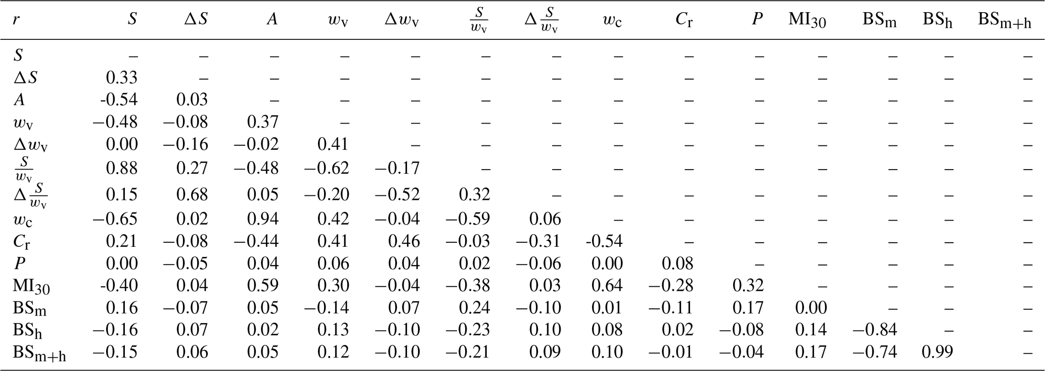
Table A2Pearson correlation coefficients (r) for the independent variables used in our statistical analysis in Hill Gulch. Independent variables include channel slope (S), ΔS, contributing area (A), valley width (wv), change in valley width (Δwv), slope ∕ width ratio (), change in slope ∕ width ratio (), channel width (wc), confinement ratio (Cr), total precipitation (P), maximum 30 min intensity (MI30), percent burned at moderate severity (BSm), percent burned at high severity (BSh), and percent burned at moderate-to-high severity (BSm+h).
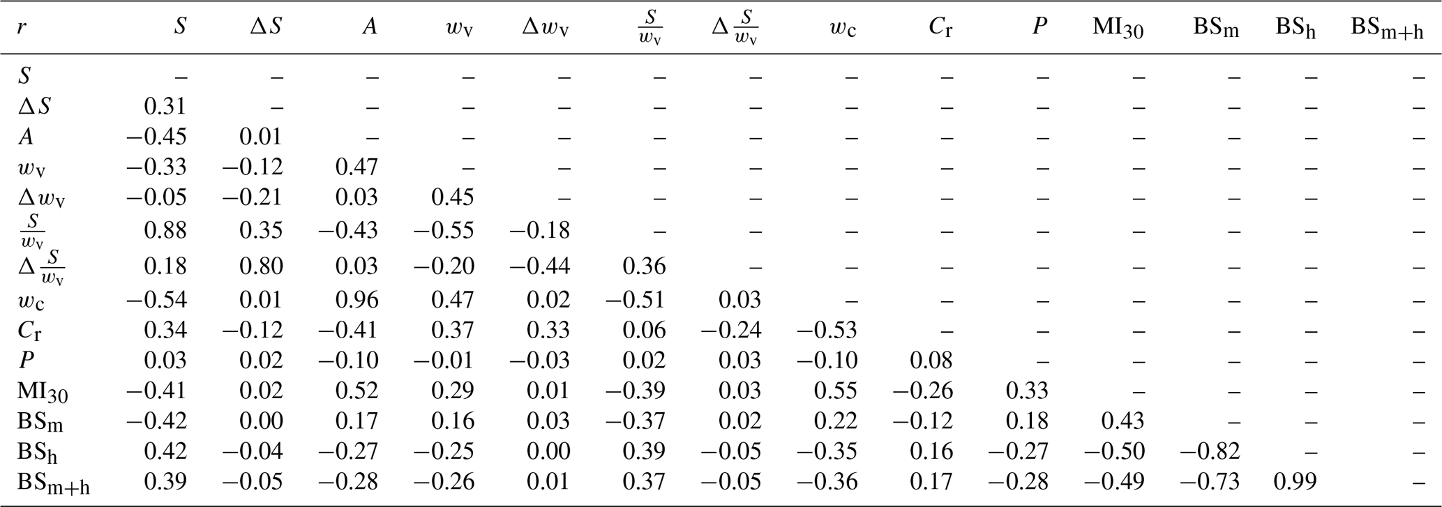

Figure A1Total deposition for each valley bottom segment in Hill Gulch for (a) 201210–201307, (b) 201307–201310, (c) 201310–201409, and (d) 201409–201506. Calculated volumes are not reported for the transparent segments due to unrealistically wide valley widths, repeat excavations, or the ground surface not being reliably determined.
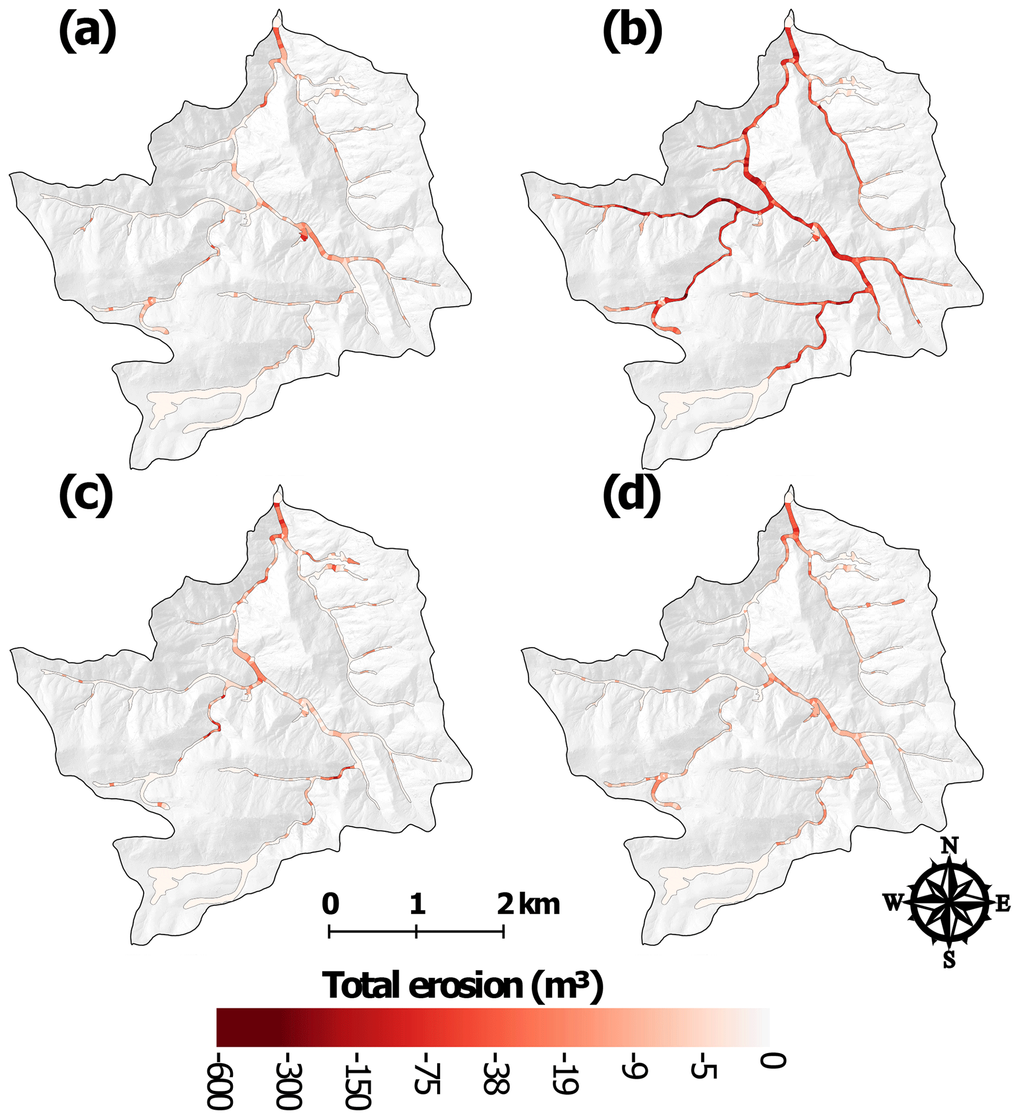
Figure A2Total erosion for each valley bottom segment in Hill Gulch for (a) 201210–201307, (b) 201307–201310, (c) 201310–201409, and (d) 201409–201506. Calculated volumes are not reported for the transparent segments due to unrealistically wide valley widths, repeat excavations, or the ground surface not being reliably determined.

Figure A3Total deposition for each valley bottom segment in Skin Gulch for (a) 201210–201307, (b) 201307–201310, (c) 201310–201409, and (d) 201409–201506. Calculated volumes are not reported for the transparent segments due to unrealistically wide valley widths, repeat excavations, or the ground surface not being reliably determined.
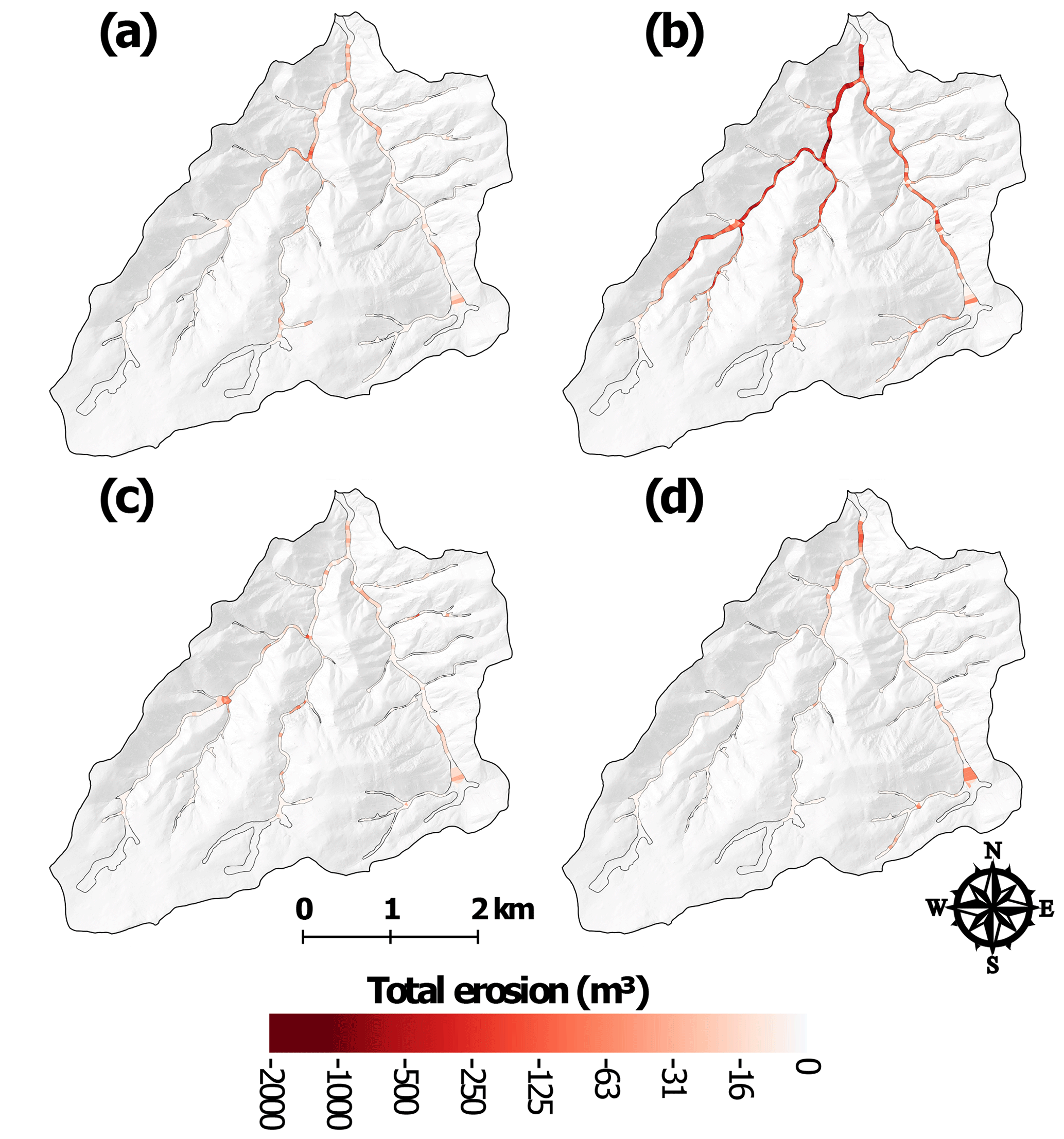
Figure A4Total erosion for each valley bottom segment in Skin Gulch for (a) 201210–201307, (b) 201307–201310, (c) 201310–201409, and (d) 201409–201506. Calculated volumes are not reported for the transparent segments due to unrealistically wide valley widths, repeat excavations, or the ground surface not being reliably determined.
DJB performed the analyses, collected field data, and wrote the paper. PAN and LHM assisted with the analysis and interpretation of data and writing and editing of the paper.
The authors declare that they have no conflict of interest.
Airborne laser scanning was provided by the National Ecological Observatory Network, a project sponsored by the National Science Foundation. This material is based in part upon work supported by the National Science Foundation under grant no. DBI-0752017. Constructive reviews from the two anonymous reviewers helped to improve the paper.
This research has been supported by the National Science Foundation, Division of Emerging Frontiers in Research and Innovation (grant nos. 1250205 and 1339928), the National Science Foundation, Division of Earth Sciences (grant no. 1419223), and the U.S. Department of Agriculture, National Institute of Food and Agriculture (grant no. 1003276), the Arapaho Roosevelt National Forest, and the U.S. Department of Agriculture Forest Service National Stream and Aquatic Ecology Center.
This paper was edited by Greg Hancock and reviewed by two anonymous referees.
Abbott, J. T.: Geology of Precambrian rocks and isotope geochemistry of shear zones in the Big Narrows area, northern Front Range, Colorado, US Geological Survey, Open-File Report OF-70-1, 1970. a
Abbott, J. T.: Geologic map of the Big Narrows quadrangle, Larimer County, Colorado, US Geological Survey, Geologic Quadrangle Map GQ-1323, 1976. a
Abrahams, E. R., Kaste, J. M., Ouimet, W., and Dethier, D. P.: Asymmetric hillslope erosion following wildfire in Fourmile Canyon, Colorado, Earth Surf. Process. Landf., 43, 2009–2021, 2018. a
Anderson, H. W.: Fire effects on water supply, floods, and sedimentation, in: Proceedings Tall Timbers Fire Ecology Conference, 249–260, 1976. a
Baker, V. and Costa, J.: Flood power, in: Catastrophic Flooding, edited by: Baker, V. and Costa, J., 1–21, Allen and Unwin, 1987. a
Bangen, S., Hensleigh, J., McHugh, P., and Wheaton, J.: Error modeling of DEMs from topographic surveys of rivers using fuzzy inference systems, Water Resour. Res., 52, 1176–1193, https://doi.org/10.1002/2015WR018299, 2016. a
Benavides-Solorio, J. and MacDonald, L. H.: Post-fire runoff and erosion from simulated rainfall on small plots, Colorado Front Range, Hydrol. Process., 15, 2931–2952, https://doi.org/10.1002/hyp.383, 2001. a
Benavides-Solorio, J. and MacDonald, L. H.: Measurement and prediction of post-fire erosion at the hillslope scale, Colorado Front Range, Int. J. Wildland Fire, 14, 457–474, https://doi.org/10.1071/WF05042, 2005. a, b, c
Benda, L. and Dunne, T.: Stochastic forcing of sediment routing and storage in channel networks, Water Resour. Res., 33, 2865–2880, https://doi.org/10.1029/97WR02387, 1997. a
Bieger, K., Rathjens, H., Allen, P. M., and Arnold, J. G.: Development and evaluation of bankfull hydraulic geometry relationships for the physiographic regions of the United States, J. Am. Water Resour. Assoc., 51, 842–858, 2015. a
Braddock, W. A., Abbott, J. T., Connor, J. J., and Swann, G. A.: Geologic map of the Poudre Park quadrangle, Larimer County, Colorado, US Geological Survey, Geologic Quadrangle Map GQ-1620, 1988. a
Brogan, D. J.: Spatial and temporal channel changes across the watershed scale following wildfire and floods, PhD dissertation, Department of Civil and Engineering. Colorado State University, Fort Collins, CO, 248 pp., 2018. a, b, c
Brogan, D. J., Nelson, P. A., and MacDonald, L. H.: Reconstructing extreme post-wildfire floods: a comparison of convective and mesoscale events, Earth Surf. Process. Landf., 42, 2505–2522, https://doi.org/10.1002/esp.4194, 2017. a, b, c, d, e, f, g, h, i, j, k, l
Brogan, D. J., MacDonald, L. H., Nelson, P. A., and Morgan, J. A.: Geomorphic complexity and sensitivity in channels to fire and floods in mountain catchments, Geomorphology, 337, 53–68, https://doi.org/10.1016/j.geomorph.2019.03.031, 2019. a, b, c, d, e, f, g, h, i, j, k, l, m, n, o, p, q, r, s, t, u, v
Brunsden, D. and Thornes, J.: Landscape sensitivity and change, Trans. Inst. British Geogr., 4, 463–484, https://doi.org/10.2307/622210, 1979. a
Cammeraat, E. L.: Scale dependent thresholds in hydrological and erosion response of a semi-arid catchment in southeast Spain, Agr. Ecosyst. Environ., 104, 317–332, https://doi.org/10.1016/j.agee.2004.01.032, 2004. a
Cannon, S. H., Kirkham, R. M., and Parise, M.: Wildfire-related debris-flow initiation processes, Storm King Mountain, Colorado, Geomorphology, 39, 171–188, https://doi.org/10.1016/S0169-555X(00)00108-2, 2001. a
Carling, P. and Beven, K.: The Hydrology, Sedimentology and Geomorphological Implications of Floods: an Overview, in: Floods: Hydrological, Sedimentological and Geomorphological Implications, John Wiley & Sons New York, 1–9, 1989. a
Costa, J. E. and O'Connor, J. E.: Geomorphically Effective Floods, in: Natural and Anthropogenic Influences in Fluvial Geomorphology, edited by: Costa, J. E., Miller, A. J., Potter, K. W., and Wilcock, P. R., 45–56, American Geophysical Union, https://doi.org/10.1029/GM089p0045, 1995. a
Cotrufo, M. F., Boot, C. M., Kampf, S., Nelson, P. A., Brogan, D. J., Covino, T., Haddix, M. L., MacDonald, L. H., Rathburn, S., Ryan-Bukett, S., Schmeer, S., and Hall, E.: Redistribution of pyrogenic carbon from hillslopes to stream corridors following a large montane wildfire, Global Biogeochem. Cy., 30, 1348–1355, https://doi.org/10.1002/2016GB005467, 2016. a
Doehring, D. O.: The effect of fire on geomorphic processes in the San Gabriel Mountains, California, Rocky Mountain Geol., 7, 43–65, 1968. a, b
Ebel, B. A., Moody, J. A., and Martin, D. A.: Hydrologic conditions controlling runoff generation immediately after wildfire, Water Resour. Res., 48, W03529, https://doi.org/10.1029/2011WR011470, 2012. a
Elliot, W. J.: WEPP internet interfaces for forest erosion prediction, J. Am. Water Resour. Assoc., 40, 299–309, https://doi.org/10.1111/J.1752-1688.2004.TB01030.X, 2004. a
Elliot, W. J., Miller, M. E., and Enstice, N.: Targeting forest management through fire and erosion modelling, Int. J. Wildland Fire, 25, 876–887, https://doi.org/10.1071/WF15007, 2016. a
Filippelli, S.: unpublished data, Colorado State University, 2015. a
Fryirs, K. A.: River sensitivity: A lost foundation concept in fluvial geomorphology, Earth Surf. Process. Landf., 42, 55–70, https://doi.org/10.1002/esp.3940, 2017. a
Fuller, I. C.: Geomorphic impacts of a 100-year flood: Kiwitea Stream, Manawatu catchment, New Zealand, Geomorphology, 98, 84–95, https://doi.org/10.1016/j.geomorph.2007.02.026, 2008. a
Gabet, E. J. and Dunne, T.: Sediment detachment by rain power, Water Resour. Res., 39, 1002, https://doi.org/10.1029/2001WR000656, 2003. a
Gartner, J. D., Dade, W. B., Renshaw, C. E., Magilligan, F. J., and Buraas, E. M.: Gradients in stream power influence lateral and downstream sediment flux in floods, Geology, 43, 983–986, https://doi.org/10.1130/G36969.1, 2015. a, b
Gilbert, J. T., Macfarlane, W. W., and Wheaton, J. M.: The Valley Bottom Extraction Tool (V-BET): A GIS tool for delineating valley bottoms across entire drainage networks, Comput. Geosci., 97, 1–14, https://doi.org/10.1016/j.cageo.2016.07.014, 2016. a
Goodrich, D., Canfield, H. E., Burns, I. S., Semmens, D., Miller, S., Hernandez, M., Levick, L., Guertin, D., and Kepner, W.: Rapid post-fire hydrologic watershed assessment using the AGWA GIS-based hydrologic modeling tool, in: Managing Watersheds for Human and Natural Impacts: Engineering, Ecological, and Economic Challenges, edited by: Moglen, G. E., 1–12, American Society of Civil Engineers, 2005. a
Hamilton, E., Horton, J., Rowe, P., and Reimann, L.: Fire-flood sequences on the San Dimas Experimental Forest, Forest Service – U.S. Department of Agriculture, California Forest and Range Experiment Station, Technical Paper No. 6, 1954. a
Hartzell, P. J., Gadomski, P. J., Glennie, C. L., Finnegan, D. C., and Deems, J. S.: Rigorous error propagation for terrestrial laser scanning with application to snow volume uncertainty, J. Glaciol., 61, 1147–1158, https://doi.org/10.3189/2015JoG15J031, 2015. a
Henkle, J. E., Wohl, E., and Beckman, N.: Locations of channel heads in the semiarid Colorado Front Range, USA, Geomorphology, 129, 309–319, 2011. a
Heritage, G. L., Milan, D. J., Large, A. R., and Fuller, I. C.: Influence of survey strategy and interpolation model on DEM quality, Geomorphology, 112, 334–344, https://doi.org/10.1016/j.geomorph.2009.06.024, 2009. a
Hodgson, M. E. and Bresnahan, P.: Accuracy of airborne LiDAR-derived elevation, Photogr. Eng. Remote Sens., 70, 331–339, https://doi.org/10.14358/PERS.70.3.331, 2004. a
HPF BAER Report: High Park Fire Burned Area Emergency Response (BAER) Report, Department of Transportation, Larimer County, Natural Resources Conservation Service, U.S. Forest Service, 25 pp., 2012. a
Huffman, E. L., MacDonald, L. H., and Stednick, J. D.: Strength and persistence of fire-induced soil hydrophobicity under ponderosa and lodgepole pine, Colorado Front Range, Hydrol. Process., 15, 2877–2892, https://doi.org/10.1002/hyp.379, 2001. a
Inbar, M., Tamir, M. I., and Wittenberg, L.: Runoff and erosion processes after a forest fire in Mount Carmel, a Mediterranean area, Geomorphology, 24, 17–33, https://doi.org/10.1016/S0169-555X(97)00098-6, 1998. a
Isenburg, M.: LAStools – fast tools to catch reality, available at: http://lastools.org, last access: 13 May 2015. a, b
Jin, S., Yang, L., Danielson, P., Homer, C., Fry, J., and Xian, G.: A comprehensive change detection method for updating the National Land Cover Database to circa 2011, Remote Sens. Environ., 132, 159–175, https://doi.org/10.1016/j.rse.2013.01.012, 2013. a
Kampf, S. K., Brogan, D. J., Schmeer, S., MacDonald, L. H., and Nelson, P. A.: How do geomorphic effects of rainfall vary with storm type and spatial scale in a post-fire landscape?, Geomorphology, 273, 39–51, https://doi.org/10.1016/j.geomorph.2016.08.001, 2016. a, b, c, d, e, f
Kean, J. W., Staley, D. M., and Cannon, S. H.: In situ measurements of post-fire debris flows in southern California: Comparisons of the timing and magnitude of 24 debris-flow events with rainfall and soil moisture conditions, J. Geophys. Res.-Earth Surf., 116, F04019, https://doi.org/10.1029/2011JF002005, 2011. a
Lague, D., Brodu, N., and Leroux, J.: Accurate 3D comparison of complex topography with terrestrial laser scanner: Application to the Rangitikei canyon (NZ), ISPRS J. Photogr. Remote Sens., 82, 10–26, https://doi.org/10.1016/j.isprsjprs.2013.04.009, 2013. a
Lane, S. N., Reid, S. C., Westaway, R. M., and Hicks, D. M.: Remotely sensed topographic data for river channel research: the identification, explanation and management of error, in: Spatial Modelling of the Terrestrial Environment, edited by: Kelly, R., Barr, S., and Drake, N., 113–136, John Wiley & Sons, Ltd: West Sussex, UK, 2004. a
Larsen, I. J. and MacDonald, L. H.: Predicting postfire sediment yields at the hillslope scale: Testing RUSLE and Disturbed WEPP, Water Resour. Res., 43, W11412, https://doi.org/10.1029/2006WR005560, 2007. a
Larsen, I. J., MacDonald, L. H., Brown, E., Rough, D., Welsh, M. J., Pietraszek, J. H., Libohova, Z., de Dios Benavides-Solorio, J., and Schaffrath, K.: Causes of post-fire runoff and erosion: water repellency, cover, or soil sealing?, Soil Sci. Soc. Am. J., 73, 1393–1407, https://doi.org/10.2136/sssaj2007.0432, 2009. a
Legleiter, C. J., Lawrence, R. L., Fonstad, M. A., Marcus, W. A., and Aspinall, R.: Fluvial response a decade after wildfire in the northern Yellowstone ecosystem: a spatially explicit analysis, Geomorphology, 54, 119–136, https://doi.org/10.1016/S0169-555X(02)00332-X, 2003. a
Magilligan, F. J., Buraas, E., and Renshaw, C.: The efficacy of stream power and flow duration on geomorphic responses to catastrophic flooding, Geomorphology, 228, 175–188, https://doi.org/10.1016/j.geomorph.2014.08.016, 2015. a
Mandlburger, G., Otepka, J., Karel, W., Wagner, W., and Pfeifer, N.: Orientation and processing of airborne laser scanning data (OPALS) – Concept and first results of a comprehensive ALS software, Int. Arch. Photogr. Remote Sens. Spatial Info. Sci., 38, 55–60, 2009. a
McGuire, L. A., Kean, J. W., Staley, D. M., Rengers, F. K., and Wasklewicz, T. A.: Constraining the relative importance of raindrop-and flow-driven sediment transport mechanisms in postwildfire environments and implications for recovery time scales, J. Geophys. Res.-Earth Surf., 121, 2211–2237, 2016. a
McGuire, L. A., Rengers, F. K., Kean, J. W., and Staley, D. M.: Debris flow initiation by runoff in a recently burned basin: Is grain-by-grain sediment bulking or en masse failure to blame?, Geophys. Res. Lett., 44, 7310–7319, 2017. a
McKean, J., Nagel, D., Tonina, D., Bailey, P., Wright, C. W., Bohn, C., and Nayegandhi, A.: Remote sensing of channels and riparian zones with a narrow-beam aquatic-terrestrial LIDAR, Remote Sens., 1, 1065–1096, https://doi.org/10.3390/rs1041065, 2009. a
Meyer, G. A., Wells, S. G., Balling Jr., R. C., and Jull, A. T.: Response of alluvial systems to fire and climate change in Yellowstone National Park, Nature, 357, 147, https://doi.org/10.1038/357147a0, 1992. a
Meyer, G. A., Wells, S. G., and Jull, A. J. T.: Fire and alluvial chronology in Yellowstone National Park: climatic and intrinsic controls on Holocene geomorphic processes, Geol. Soc. Am. Bull., 107, 1211–1230, https://doi.org/10.1130/0016-7606(1995)107<1211:FAACIY>2.3.CO;2, 1995. a
Milan, D. J., Heritage, G. L., Large, A. R., and Fuller, I. C.: Filtering spatial error from DEMs: Implications for morphological change estimation, Geomorphology, 125, 160–171, https://doi.org/10.1016/j.geomorph.2010.09.012, 2011. a, b, c
Miller, A. J.: Valley morphology and boundary conditions influencing spatial patterns of flood flow, in: Natural and anthropogenic influences in fluvial geomorphology, edited by: Costa, J. E., Miller, A. J., Potter, K. W., and Wilcock, P. R., 57–81, Wiley Online Library, https://doi.org/10.1029/GM089p0057, 1995. a
Miller, M. E., MacDonald, L. H., Robichaud, P. R., and Elliot, W. J.: Predicting post-fire hillslope erosion in forest lands of the western United States, Int. J. Wildland Fire, 20, 982–999, https://doi.org/10.1071/WF09142, 2011. a, b
Montgomery, D. R. and Buffington, J. M.: Channel-reach morphology in mountain drainage basins, Geol. Soc. Am. Bull., 109, 596–611, https://doi.org/10.1130/0016-7606(1997)109<0596:CRMIMD>2.3.CO;2, 1997. a, b
Moody, J. A.: Residence times and alluvial architecture of a sediment superslug in response to different flow regimes, Geomorphology, 294, 40–57, https://doi.org/10.1016/j.geomorph.2017.04.012, 2017. a
Moody, J. A. and Kinner, D. A.: Spatial structures of stream and hillslope drainage networks following gully erosion after wildfire, Earth Surf. Process. Landf., 31, 319–337, https://doi.org/10.1002/esp.1246, 2006. a
Moody, J. A. and Martin, D. A.: Initial hydrologic and geomorphic response following a wildfire in the Colorado Front Range, Earth Surf. Process. Landf., 26, 1049–1070, https://doi.org/10.1002/esp.253, 2001. a, b, c, d
Moody, J. A. and Martin, D. A.: Wildfire impacts on reservoir sedimentation in the western United States, in: Proceedings of the Ninth International Symposium on River Sedimentation, 1095–1102, Tsinghua University Press China, 2004. a
Moody, J. A. and Martin, D. A.: Synthesis of sediment yields after wildland fire in different rainfall regimes in the western United States, Int. J. Wildland Fire, 18, 96–115, https://doi.org/10.1071/WF07162, 2009. a
Moody, J. A., Shakesby, R. A., Robichaud, P. R., Cannon, S. H., and Martin, D. A.: Current research issues related to post-wildfire runoff and erosion processes, Earth-Sci. Rev., 122, 10–37, 2013. a, b, c, d
Morris, S. E. and Moses, T. A.: Forest fire and the natural soil erosion regime in the Colorado Front Range, Ann. Assoc. Am. Geogr., 77, 245–254, https://doi.org/10.1111/j.1467-8306.1987.tb00156.x, 1987. a
Nagel, D., Buffington, J., Parkes, S., Wenger, S., and Goode, J.: A Landscape Scale Valley Confinement Algorithm: Delineating Unconfined Valley Bottoms for Geomorphic, Aquatic, and Riparian Applications, US Dept of Agriculture, Forest Service, RMRS-GTR 321, Fort Collins, CO, p. 42, https://doi.org/10.2737/RMRS-GTR-321, 2014. a
Nardi, L. and Rinaldi, M.: Spatio-temporal patterns of channel changes in response to a major flood event: the case of the Magra River (central–northern Italy), Earth Surf. Process. Landf., 40, 326–339, https://doi.org/10.1002/esp.3636, 2015. a, b
Nelson, P. A. and Brogan, D. J.: Dataset associated with “Spatial and temporal patterns of sediment storage and erosion following a wildfire and extreme flood”, Data set, https://doi.org/10.25675/10217/193080, 2019. a
Nuth, C. and Kääb, A.: Co-registration and bias corrections of satellite elevation data sets for quantifying glacier thickness change, The Cryosphere, 5, 271–290, https://doi.org/10.5194/tc-5-271-2011, 2011. a, b
Onda, Y., Dietrich, W. E., and Booker, F.: Evolution of overland flow after a severe forest fire, Point Reyes, California, Catena, 72, 13–20, https://doi.org/10.1016/j.catena.2007.02.003, 2008. a
Orem, C. A. and Pelletier, J. D.: Quantifying the time scale of elevated geomorphic response following wildfires using multi-temporal LiDAR data: An example from the Las Conchas fire, Jemez Mountains, New Mexico, Geomorphology, 232, 224–238, 2015. a, b
Passalacqua, P., Belmont, P., Staley, D. M., Simley, J. D., Arrowsmith, J. R., Bode, C. A., Crosby, C., DeLong, S. B., Glenn, N. F., Kelly, S. A., Lague, D., Sangireddy, H., Schaffrath, K., Tarboton, D. G., Wasklewicz, T., and Wheaton, J. M.: Analyzing high resolution topography for advancing the understanding of mass and energy transfer through landscapes: A review, Earth-Sci. Rev., 148, 174–193, https://doi.org/10.1016/j.earscirev.2015.05.012, 2015. a, b
Pelletier, J. D. and Orem, C. A.: How do sediment yields from post-wildfire debris-laden flows depend on terrain slope, soil burn severity class, and drainage basin area? Insights from airborne-LiDAR change detection, Earth Surf. Process. Landf., 39, 1822–1832, https://doi.org/10.1002/esp.3570, 2014. a
Phillips, J. D. and Van Dyke, C.: Principles of geomorphic disturbance and recovery in response to storms, Earth Surf. Process. Landf., 41, 971–979, https://doi.org/10.1002/esp.3912, 2016. a
Prosser, I. P. and Williams, L.: The effect of wildfire on runoff and erosion in native Eucalyptus forest, Hydrol. Process., 12, 251–265, https://doi.org/10.1002/(SICI)1099-1085(199802)12:2<251::AID-HYP574>3.0.CO;2-4, 1998. a
Rathburn, S. L., Shahverdian, S. M., and Ryan, S. E.: Post-disturbance sediment recovery: Implications for watershed resilience, Geomorphology, 305, 61–75, https://doi.org/10.1016/j.geomorph.2017.08.039, 2017. a
Renard, K. G., Foster, G. R., Weesies, G. A., McCool, D. K., and Yoder, D. C.: Predicting soil erosion by water: a guide to conservation planning with the Revised Universal Soil Loss Equation (RUSLE), US Government Printing Office Washington, DC, 1997. a
Reneau, S. L., Katzman, D., Kuyumjian, G. A., Lavine, A., and Malmon, D. V.: Sediment delivery after a wildfire, Geology, 35, 151–154, https://doi.org/10.1130/G23288A.1, 2007. a, b
Rengers, F., McGuire, L., Kean, J. W., Staley, D. M., and Hobley, D.: Model simulations of flood and debris flow timing in steep catchments after wildfire, Water Resour. Res., 52, 6041–6061, 2016a. a
Rengers, F., Tucker, G., Moody, J., and Ebel, B.: Illuminating wildfire erosion and deposition patterns with repeat terrestrial lidar, J. Geophys. Res.-Earth Surf., 121, 588–608, https://doi.org/10.1002/2015JF003600, 2016b. a
Rhoades, C. C., Entwistle, D., and Butler, D.: The influence of wildfire extent and severity on streamwater chemistry, sediment and temperature following the Hayman Fire, Colorado, Int. J. Wildland Fire, 20, 430–442, https://doi.org/10.1071/WF09086, 2011. a
Rinaldi, M., Surian, N., Comiti, F., and Bussettini, M.: A method for the assessment and analysis of the hydromorphological condition of Italian streams: the Morphological Quality Index (MQI), Geomorphology, 180, 96–108, https://doi.org/10.1016/j.geomorph.2012.09.009, 2013. a
Robichaud, P. R., Beyers, J. L., and Neary, D. G.: Evaluating the effectiveness of postfire rehabilitation treatments, USDA Forest Service, RMRS-GTR-63, Fort Collins, CO, 2000. a
Robichaud, P. R., Elliot, W. J., Pierson, F. B., Hall, D. E., and Moffet, C. A.: Predicting postfire erosion and mitigation effectiveness with a web-based probabilistic erosion model, Catena, 71, 229–241, https://doi.org/10.1016/j.catena.2007.03.003, 2007. a
Roering, J. J. and Gerber, M.: Fire and the evolution of steep, soil-mantled landscapes, Geology, 33, 349–352, https://doi.org/10.1130/G21260.1, 2005. a
Roux, C., Alber, A., Bertrand, M., Vaudor, L., and Piégay, H.: “FluvialCorridor”: A new ArcGIS toolbox package for multiscale riverscape exploration, Geomorphology, 242, 29–37, https://doi.org/10.1016/j.geomorph.2014.04.018, 2015. a, b
Santi, P. M., deWolfe, V. G., Higgins, J. D., Cannon, S. H., and Gartner, J. E.: Sources of debris flow material in burned areas, Geomorphology, 96, 310–321, https://doi.org/10.1016/j.geomorph.2007.02.022, 2008. a
Schmeer, S. R., Kampf, S. K., MacDonald, L. H., Hewitt, J., and Wilson, C.: Empirical models of annual post-fire erosion on mulched and unmulched hillslopes, CATENA, 163, 276–287, https://doi.org/10.1016/j.catena.2017.12.029, 2018. a, b, c, d, e, f, g, h, i
Schumm, S. A.: Geomorphic thresholds and complex response of drainage systems, Fluv. Geomor., 6, 69–85, 1973. a
Shakesby, R. A. and Doerr, S. H.: Wildfire as a hydrological and geomorphological agent, Earth-Sci. Rev., 74, 269–307, 2006. a, b
Smith, M., Carrivick, J., and Quincey, D.: Structure from motion photogrammetry in physical geography, Progr. Phys. Geogr., 40, 247–275, https://doi.org/10.1177/0309133315615805, 2016. a
Soil Survey Staff: Natural Resources Conservation Service, United States Department of Agriculture. Web Soil Survey, available at: https://websoilsurvey.sc.egov.usda.gov/, last access: 25 January 2018. a, b
Stoffel, M., Wyżga, B., and Marston, R. A.: Floods in mountain environments: A synthesis, Geomorphology, 272, 1–9, https://doi.org/10.1016/j.geomorph.2016.07.008, 2016. a
Stone, B.: Mapping burn severity, pine beetle infestation, and their interaction at the High Park Fire, Master's thesis, Graduate Degree Program in Ecology. Colorado State University, Fort Collins, CO, 90 pp., 2015. a
Stoof, C. R., Vervoort, R. W., Iwema, J., van den Elsen, E., Ferreira, A. J. D., and Ritsema, C. J.: Hydrological response of a small catchment burned by experimental fire, Hydrol. Earth Syst. Sci., 16, 267–285, https://doi.org/10.5194/hess-16-267-2012, 2012. a, b
Stout, J. C. and Belmont, P.: TerEx Toolbox for semi-automated selection of fluvial terrace and floodplain features from lidar, Earth Surf. Process. Landf., 39, 569–580, https://doi.org/10.1002/esp.3464, 2014. a
Surian, N., Righini, M., Lucía, A., Nardi, L., Amponsah, W., Benvenuti, M., Borga, M., Cavalli, M., Comiti, F., Marchi, L., Rinaldi, M., and Viero, A.: Channel response to extreme floods: insights on controlling factors from six mountain rivers in northern Apennines, Italy, Geomorphology, 272, 78–91, https://doi.org/10.1016/j.geomorph.2016.02.002, 2016. a
Swanson, F. J.: Fire and geomorphic processes, in: Fire Regime and Ecosystem Properties, edited by: Mooney, H., Bonnicksen, T., Christensen, N., Lotan, J., and Reiners, W., 401–444, United States Department of Agriculture Forest Service General Technical Report WO-26, 1981. a
Thomas, M. F.: Landscape sensitivity in time and space – an introduction, Catena, 42, 83–98, https://doi.org/10.1016/S0341-8162(00)00133-8, 2001. a
Thompson, C. and Croke, J.: Geomorphic effects, flood power, and channel competence of a catastrophic flood in confined and unconfined reaches of the upper Lockyer valley, southeast Queensland, Australia, Geomorphology, 197, 156–169, https://doi.org/10.1016/j.geomorph.2013.05.006, 2013. a
Tulldahl, H. M. and Larsson, H.: Lidar on small UAV for 3D mapping, in: Electro-Optical Remote Sensing, Photonic Technologies, and Applications VIII; and Military Applications in Hyperspectral Imaging and High Spatial Resolution Sensing II, International Society for Optics and Photonics, Amsterdam, Netherlands, https://doi.org/10.1117/12.2068448, 2014. a
Vericat, D., Wheaton, J. M., and Brasington, J.: Revisiting the Morphological Approach: Opportunities and Challenges with Repeat High-Resolution Topography, in: Gravel-Bed Rivers: Process and Disasters, 121–155, John Wiley & Sons, 2017. a
Wagenbrenner, J. W. and Robichaud, P. R.: Post-fire bedload sediment delivery across spatial scales in the interior western United States, Earth Surf. Process. Landf., 39, 865–876, https://doi.org/10.1002/esp.3488, 2014. a, b
Wagenbrenner, J., MacDonald, L., and Rough, D.: Effectiveness of three post-fire rehabilitation treatments in the Colorado Front Range, Hydrol. Process., 20, 2989–3006, https://doi.org/10.1002/hyp.6146, 2006. a, b
Weber, M. D. and Pasternack, G. B.: Valley-scale morphology drives differences in fluvial sediment budgets and incision rates during contrasting flow regimes, Geomorphology, 288, 39–51, https://doi.org/10.1016/j.geomorph.2017.03.018, 2017. a
Wheaton, J. M., Brasington, J., Darby, S. E., and Sear, D. A.: Accounting for uncertainty in DEMs from repeat topographic surveys: improved sediment budgets, Earth Surf. Process. Landf., 35, 136–156, https://doi.org/10.1002/esp.1886, 2010. a, b, c, d
Wicherski, W., Dethier, D. P., and Ouimet, W. B.: Erosion and channel changes due to extreme flooding in the Fourmile Creek catchment, Colorado, Geomorphology, 294, 87–98, https://doi.org/10.1016/j.geomorph.2017.03.030, 2017. a
Wilson, C., Kampf, S. K., Wagenbrenner, J. W., and MacDonald, L. H.: Rainfall thresholds for post-fire runoff and sediment delivery from plot to watershed scales, Forest Ecol. Manage., 430, 346–356, https://doi.org/10.1016/j.foreco.2018.08.025, 2018. a
Wohl, E.: Migration of channel heads following wildfire in the Colorado Front Range, USA, Earth Surf. Process. Landf., 38, 1049–1053, https://doi.org/10.1002/esp.3429, 2013. a
Wohl, E. and Scott, D. N.: Transience of channel head locations following disturbance, Earth Surf. Process. Landf., 42, 1132–1139, https://doi.org/10.1002/esp.4124, 2017. a
Wolman, M. G. and Eiler, J. P.: Reconnaissance study of erosion and deposition produced by the flood of August 1955 in Connecticut, EOS, Transactions American Geophysical Union, 39, 1–14, https://doi.org/10.1029/TR039i001p00001, 1958. a
Wright, D. B., Smith, J. A., Villarini, G., and Baeck, M. L.: Long-term high-resolution radar rainfall fields for urban hydrology, JAWRA J. Am. Water Resour. Assoc., 50, 713–734, https://doi.org/10.1111/jawr.12139, 2014. a
Writer, J. H., Hohner, A., Oropeza, J., Schmidt, A., Cawley, K. M., and Rosario-Ortiz, F. L.: Water treatment implications after the high Park wildfire, Colorado, J. Am. Water Works Assoc., 106, E189–E199, https://doi.org/10.5942/jawwa.2014.106.0055, 2014. a, b
Yager, E. M., Dietrich, W., Kirchner, J. W., and McArdell, B.: Patch dynamics and stability in steep, rough streams, J. Geophys. Res.-Earth Surf., 117, F02010, https://doi.org/10.1029/2011JF002253, 2012. a
Yochum, S. E., Sholtes, J. S., Scott, J. A., and Bledsoe, B. P.: Stream power framework for predicting geomorphic change: The 2013 Colorado Front Range flood, Geomorphology, 292, 178–192, https://doi.org/10.1016/j.geomorph.2017.03.004, 2017. a, b