the Creative Commons Attribution 4.0 License.
the Creative Commons Attribution 4.0 License.
 | 26 Jun 2019
A coupled soilscape–landform evolution model: model formulation and initial results
W. D. Dimuth P. Welivitiya
Garry R. Willgoose
Greg R. Hancock
This paper describes the coupling of the State Space Soil Production and Assessment Model (SSSPAM) soilscape evolution model with a landform evolution model to integrate soil profile dynamics and landform evolution. SSSPAM is a computationally efficient soil evolution model which was formulated by generalising the mARM3D modelling framework to further explore the soil profile self-organisation in space and time, as well as its dynamic evolution. The landform evolution was integrated into SSSPAM by incorporating the processes of deposition and elevation changes resulting from erosion and deposition. The complexities of the physically based process equations were simplified by introducing a state-space matrix methodology that allows efficient simulation of mechanistically linked landscape and pedogenesis processes for catena spatial scales. SSSPAM explicitly describes the particle size grading of the entire soil profile at different soil depths, tracks the sediment grading of the flow, and calculates the elevation difference caused by erosion and deposition at every point in the soilscape at each time step. The landform evolution model allows the landform to change in response to (1) erosion and deposition and (2) spatial organisation of the co-evolving soils. This allows comprehensive analysis of soil landform interactions and soil self-organisation. SSSPAM simulates fluvial erosion, armouring, physical weathering, and sediment deposition. The modular nature of the SSSPAM framework allows the integration of other pedogenesis processes to be easily incorporated. This paper presents the initial results of soil profile evolution on a dynamic landform. These simulations were carried out on a simple linear hillslope to understand the relationships between soil characteristics and the geomorphic attributes (e.g. slope, area). Process interactions which lead to such relationships were also identified. The influence of the depth-dependent weathering function on soilscape and landform evolution was also explored. These simulations show that the balance between erosion rate and sediment load in the flow accounts for the variability in spatial soil characteristics while the depth-dependent weathering function has a major influence on soil formation and landform evolution. The results demonstrate the ability of SSSPAM to explore hillslope- and catchment-scale soil and landscape evolution in a coupled framework.
- Article
(1863 KB) - Full-text XML
- BibTeX
- EndNote


Soil is one of the most important substances found on planet Earth. As the uppermost layer of the Earth's surface, soil supports all the terrestrial organisms ranging from microbes to plants to humans and provides the substrate for terrestrial life (Lin, 2011). Soil provides a transport and a storage medium for water and gases (e.g. carbon dioxide which influences the global climate) (Strahler and Strahler, 2006). The nature of the soil heavily influences both geomorphological and hydrological processes (Bryan, 2000). In addition to the importance of soil from an environmental standpoint, it provides a basis for human civilisation and played an important role in its advancement through the means of agricultural development (Jenny, 1941). Understanding the formation and the global distribution of soil (and its functional properties) is imperative in the quest for sustainable use of this resource.
Characterisation of soil properties at a global scale by sampling and analysis is time-consuming and prohibitively expensive due to the dynamic nature of the soil system and its complexity (Hillel, 1982). However, over the years researchers have found strong links between different soil properties and the geomorphology of the landform on which they reside (Gessler et al., 2000, 1995). Working on this relationship several statistical methods have been developed to determine and map various soil properties depending on other soil properties and geomorphology such as pedotransfer functions, geostatistical approaches, and state-factor (e.g. clorpt) approaches (Behrens and Scholten, 2006). Pedotransfer functions (PTFs) use easily measurable soil attributes such as particle size distribution, amount of organic matter, and clay content to predict hard-to-measure soil properties such as soil water content. Although very useful, PTFs need a large database of spatially distributed soil property data and require site-specific calibration (Benites et al., 2007). Geostatistical methods use a finite number of field samples to interpolate the soil property distribution over a large area. Developing soil property maps using geostatistical methods is possible for smaller spatial scales; however, soil sampling and mapping soil attributes can be prohibitively expensive and time-consuming for larger spatial domains (Scull et al., 2003). State-factor methods, such as scorpan (developed by introducing existing soil types and geographical position to the clorpt framework), use digitised existing soil maps and easily measurable soil attribute data to generate spatially distributed soil property data using mathematical concepts such as fuzzy set theory, artificial neural network, or decision tree methods (McBratney et al., 2003). However, these techniques also suffer from scalability issues and the typical need for site-specific calibration.
While spatial mapping of soil properties is important, understanding the evolution of these soil properties and processes responsible for observed spatial variability of soil properties is also important. In order to quantify these processes and predict the soil characteristics evolution through time, dynamic process-based models are required (Hoosbeek and Bryant, 1992). These mechanistic process models predict soil properties using both geomorphological attributes and various physical processes such as weathering, erosion, and bioturbation (Minasny and McBratney, 1999). ARMOUR, developed by Sharmeen and Willgoose (2006), is one of the earliest process-based pedogenesis models. ARMOUR simulated surface armouring based on erosion and size-selective entrainment of sediments driven by rainfall events and overland flow, as well as physical weathering of the soil particles which break down the surface armour layer. However, very high computational resource requirements and long run times prevented ARMOUR from performing simulations beyond short hillslopes. Subsequently Cohen et al. (2009) developed mARM by implementing a state-space matrix methodology to simplify the process-based equations and calibrated its process parameters using the results from ARMOUR. Its high computational efficiency allowed mARM to explore soil evolution characteristics on spatially distributed landforms. Through their simulations, Cohen et al. (2009) found a strong relationship between the geomorphic quantities contributing area, slope, and soil surface grading d50. Both ARMOUR and mARM simulate a surface armour layer and a semi-infinite subsurface soil layer which supplies sediments to the upper armour layer. For this reason both of these models were incapable of exploring the evolution of subsurface soil profiles. To overcome this limitation Cohen et al. (2010) developed mARM3D by incorporating multiple soil layers into the mARM modelling framework. To generalise the work of Cohen et al. (2010), Welivitiya et al. (2016) developed a new soil grading evolution model called SSSPAM (State Space Soil Production and Assessment Model), which was based on the approach of mARM3D and showed that the area–slope–d50 relationship in Cohen et al. (2009) was robust against changes in process and climate parameters and that the relationship is also true for all the subsurface soil layers, not just the surface. Although these models predict the properties of the soil profile at an individual pixel, they do not model the spatial interconnectivity between different parts of the soil catena resulting from transport-limited erosion and deposition. Lateral material movement and particle redistribution through deposition is very important in determining the soil characteristics such as soil depth and soil texture (Chittleborough, 1992; Minasny and McBratney, 2006). In order to correctly predict spatially distributed soil attributes and determine the changes in soil attributes with time, coupling soil profile evolution with landform evolution is important.
The first attempt to integrate soilscape evolution with landform evolution was done by Minasny and McBratney (1999, 2001). They used a single layer to model the influence of soil and weathering processes on landform evolution. In addition to Minasny and McBratney (1999, 2001) there are a number of conceptual frameworks found in the literature for developing coupled soil-profile–landform evolution models (Yoo and Mudd, 2008; Sommer et al., 2008). MILESD (Vanwalleghem et al., 2013) is a model which can simulate soil profile evolution coupled with landform evolution. MILESD is built upon the conceptual framework of landscape-scale models for soil redistribution by Minasny and McBratney (1999, 2001) and the pedon-scale soil formation model developed by Salvador-Blanes et al. (2007). In MILESD the soil profile is divided into four layers containing the bottommost bedrock layer and three soil layers above it representing the A, B, and C soil horizons. MILESD was used to model soil development over 60 000 years for a field site in Werrikimbe National Park, Australia (Vanwalleghem et al., 2013). They matched trends observed in the field such as the spatial variation of soil thickness, soil texture, and organic carbon content. A limitation of MILESD is that it only uses three layers to represent the soil profile. Recently the soil evolution module used in MILESD has been modified to incorporate additional layers and has been combined with the landform evolution model LAPSUS to develop a new coupled soilscape–landform evolution model, LORICA (Temme and Vanwalleghem, 2015). They found similar results for soil–landform interaction and evolution similar to MILESD simulation results.
Since only three layers were used in MILESD, the representation of the particle size distribution down the soil profile was limited. Although LORICA incorporated additional soil layers into the MILESD modelling framework, detailed exploration of soil profile evolution or interactions between landform evolution and soil profile evolution has not yet been done with this model. Importantly, particle size distribution of the soil can be used as a proxy for various soil attributes such as the soil moisture content (Arya and Paris, 1981; Schaap et al., 2001). The main objective of this paper is to present a new soilscape evolution model capable of predicting the particle size distribution of the entire soil profile by integrating a previously developed soil grading evolution model into a landscape evolution model.
Here we present the methodology for incorporating sediment transport, deposition, and elevation changes of the landform into the SSSPAM modelling framework to create a coupled soilscape–landform evolution model. Detailed information regarding the development and testing of the SSSPAM soil grading evolution model is provided in previous papers by the authors (Cohen et al., 2010; Welivitiya et al., 2016). The main focus of this paper is to incorporate landform evolution into the SSSPAM framework. In addition to the model development we also present the initial results of coupled soilscape–landform evolution exemplified on a linear hillslope.
The introduction of a landform into the SSSPAM framework is done using a digital elevation model. The structure of the landform evolution model follows that for transport-limited erosion (Willgoose et al., 1991) but modified so as to facilitate its coupling with the soilscape soil grading evolution model SSSPAM described in Welivitiya et al. (2016). Here a regular square grid digital elevation model was used and converted into a two-dimensional array which can be easily processed and analysed in the Python/Cython programming language. Using the steepest-slope criterion (Tarboton, 1997) the flow direction and the slope value of each pixel was determined. Then using the created flow direction matrix, the contributing area of each pixel was determined using the D8 method (O'Callaghan and Mark, 1984) with a recursive algorithm.
The soil profile evolution of each pixel is determined using the interactions between the soil profile and the flowing water at the surface. Figure 1 shows these layers and their potential interactions. This is similar to the schematic for the stand-alone soil grading evolution model but is different in that the erosion/deposition at the surface is a result of the imbalance between upslope and downslope sediment transport. The water layer acts as the medium in which soil particle entrainment or deposition occurs depending on the transport capacity of the water at that pixel. The water provides the lateral coupling across the landform, by the sediment transport process. The soil profile is modelled as several layers to reflect the fact that the soil grading changes with soil depth depending on the weathering characteristics of soil. Erosion of soil and/or sediment deposition occurs at the surface soil layer (surface armour layer).

SSSPAM uses the state-space matrix approach to evolve the soil grading through the soil profile. The state-space matrix methodology used for soilscape evolution is presented in detail elsewhere (Cohen et al., 2009, 2010; Welivitiya et al., 2016) and will not be discussed in detail here. Using this method a range of processes (e.g. erosion, weathering, deposition) can be represented and applied so that the total change in soil layers and their properties can be determined (Cohen et al., 2009, 2010). Once the erosion and deposition mass is determined, elevation changes are calculated and the digital elevation model is modified accordingly. Once the algorithm completes modifying the digital elevation model matrix, the calculation of flow direction and contributing area is done and the process is repeated until a given number of iterations (evolution time) is reached.
2.1 Characterising erosion and deposition
As described in Welivitiya et al. (2016), the SSSPAM soil grading evolution model used a detachment-limited erosion model to calculate the amount of erosion. In order to simulate deposition and to differentiate between erosion and deposition, a transport-limited model is incorporated into the soil grading evolution model SSSPAM. Before calculating the erosion or deposition at a pixel (i.e. grid cell/node), we determine the transport capacity of the flow at that particular pixel. The transport capacity determines if the pixel is being subjected to erosion or deposition. The calculation of the transport capacity at each pixel is done according to the empirical equation presented by Zhang et al. (2011), which was determined by flume-scale sediment detachment experiments. The transport capacity at a pixel (node) Tc (kg s−1) is given by
where Q is the discharge per unit width (m3 s−1 m−1) at the pixel, S is the slope gradient (m m−1), and is the median diameter of the sediment load in the flow (m); K1, δ1, δ2, and δ3 are constants determined empirically; and ω is the flow width (m) at the pixel. Q is
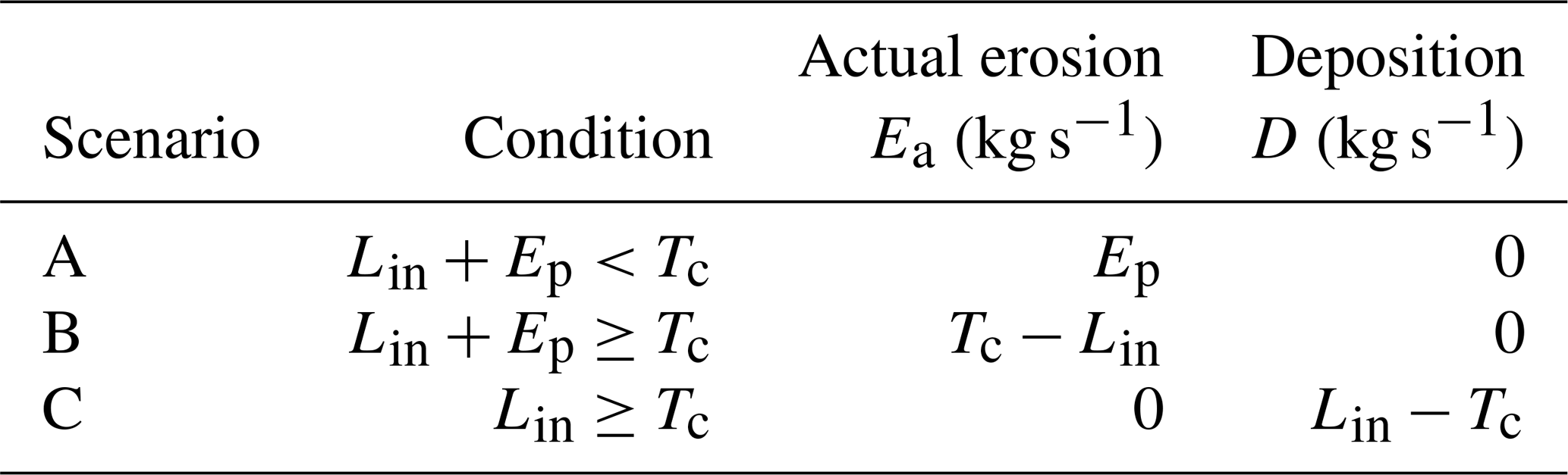
where r is runoff excess generation (m3 s−1 m−2) and Ac is contributing area (m2) of that pixel. Using their flume particle detachment experiments Zhang et al. (2011) determined that K1=2382.32, δ1=1.26, δ2=1.63, and gave the best fit to their experimental results (with an R2 value of 0.98). If ψin is the mass vector of the incoming sediment to the pixel, then is the total mass of incoming sediments to that pixel transported by water. Here ψin represents the cumulative outflow sediment mass vectors of upstream pixels (∑ψout) which drain into the pixel in question and is determined using the flow direction matrix mentioned earlier. Using this method, SSSPAM can model the total mass of the eroded sediment as well as the grading of the eroded material. Depending on the total incoming sediment load at the pixel Lin, the transport capacity Tc of the flow, and the potential total erosion mass Ep, the amount of actual erosion Ea (kg s−1) or deposition D (kg s−1) can be determined according to Table 1. The scenarios A and B (in Table 1) lead to erosion and armouring while scenario C leads to deposition.
2.2 Erosion, armouring, and soil profile restructuring
The calculation of potential erosion Ep and armouring of the soil surface is done as in Welivitiya et al. (2016) and Cohen et al. (2009). The actual erosion Ea is then determined by adjusting the potential erosion Ep according to scenarios A or B (Table 1). When calculating the actual erosion Ea we determine only the total mass of the erodible material (although it should be remembered that total erosion is a function of the transport capacity which is in turn a function of the grading d50). The actual erosion mass vector Ge is determined using the total soil surface mass grading vector G and erosion transition matrix A. The method utilised to generate this erosion transition matrix A is identical to that described in detail in Welivitiya et al. (2016) and Cohen et al. (2009) and will not be discussed in detail here. Briefly, the methodology is a size-selective entrainment of soil particles from the surface due to erosion leaving the surface armour layer enriched with coarser material. It is similar to the approach of Parker and Klingeman (1982) which Willgoose and Sharmeen (2006) showed was the best fit to their field data for their ARMOUR surface armouring model. The eroded material is added to the sediment load flowing into the pixel and can be given as the outflow sediment mass vector ψout.
The actual depth of erosion ΔhE (m) is calculated using the equation
where Rx and Ry are the grid cell dimensions (m) in the two cardinal direction (pixel resolution), and ρs is the bulk density of the soil material (kg m−3). Here we assume that the bulk density ρs remains constant regardless of the soil grading and over the simulation time of the simulation.
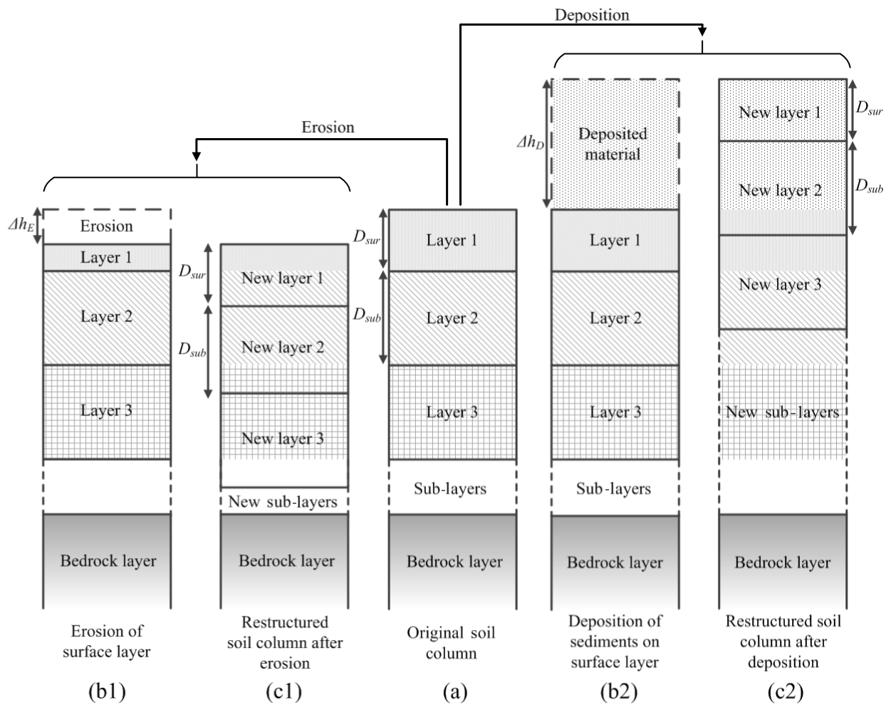
Figure 2Erosion, deposition, and the restructuring of the soil profile: (a) original soil profile, (b1, c1) for erosion, and (b2, c2) for deposition.
As described by the above equations, mass is removed from the surface armour layer into the water flowing above. In SSSPAM, mass conservation of the surface armour layer is achieved by adding a portion of soil from the first subsurface layer to the surface armour layer equal to the mass entrained into the water flow. It is important to note that the materials resupplied to the surface armour have the same soil grading as the subsurface layer. So both small particles and large particles are resupplied to the armour layer. Most of the time the net effect of this material resupply and the size-selective erosion will be enrichment of larger particles and armour strengthening. Depending on the depth-dependent weathering function, the relative coarseness of the subsurface layers can be less compared to armour layer. But once the armour layer is reconfigured with the added material from below and removal of small particles through erosion, again the net effect is armour strengthening. More detailed description of this process can be found in Cohen et al. (2009) and Welivitiya et al. (2016)
This material resupply propagates down the soil profile (one soil layer supplying material to the layer above and receiving material from the layer below) all the way to the bedrock layer, which is semi-infinite in thickness. Since the soil gradings of different layers are different to each other, this flux of material through the soil profile changes the soil grading of all the subsurface layers. Conceptually the position of the modelled soil column moves downward since all vertical distances for the soil layers are relative to the soil surface. In the case of deposition the model space would move upwards (discussed in detail later). This movement of the soil model space during erosion is illustrated in Fig. 2.
Note that erosion is limited by the imbalance between sediment transport capacity and the amount of the sediment load in the flow as well as the threshold diameter of the particle which can be entrained (Shields shear threshold; see Cohen et al., 2009, for details) by the water flow. These factors limit the potential erosion rate at a pixel. During the test simulations presented later in this paper, the depth of erosion ΔhE was always less than the surface armour layer thickness Dsur (Fig. 2a) and the rearrangement of the soil grading of all the layers was straightforward.
2.3 Sediment deposition
If the total mass of incoming sediment Lin is higher than the transport capacity of the sediment transport capacity Tc at the pixel (Table 1, scenario C) deposition of sediments occurs at the pixel. The mass of deposited material is the difference between Lin and Tc. Although calculating the total mass of sediment which needs to deposit at a pixel (D) is straightforward, determining the distribution of the deposited sediments in the form of deposition mass vector Φ is somewhat complicated. The deposition mass vector Φ depends on the size distribution of the incoming sediments, which in turn depend on the erosion characteristics of the upstream pixels. The calculation of the deposition mass vector Φ is done using the deposition transition matrix J. Here Φ is defined as
where Jz,z represents the diagonal entries of J (here and after, the subscript z denotes the zth grading class), and ψz represents the elements of ψin. K is an adjustment vector which modifies the values in deposition mass vector Φ such that Φz≤ψz, with Φz being the elements of the vector Φ. The adjustment vector K ensures that deposited material from each size class is not greater than the total amount of sediment load available in the incoming sediment flow and is iteratively determined within the deposition module of SSSPAM. The following simplified example shows the need to have this adjustment vector and the method we used to calculate it.
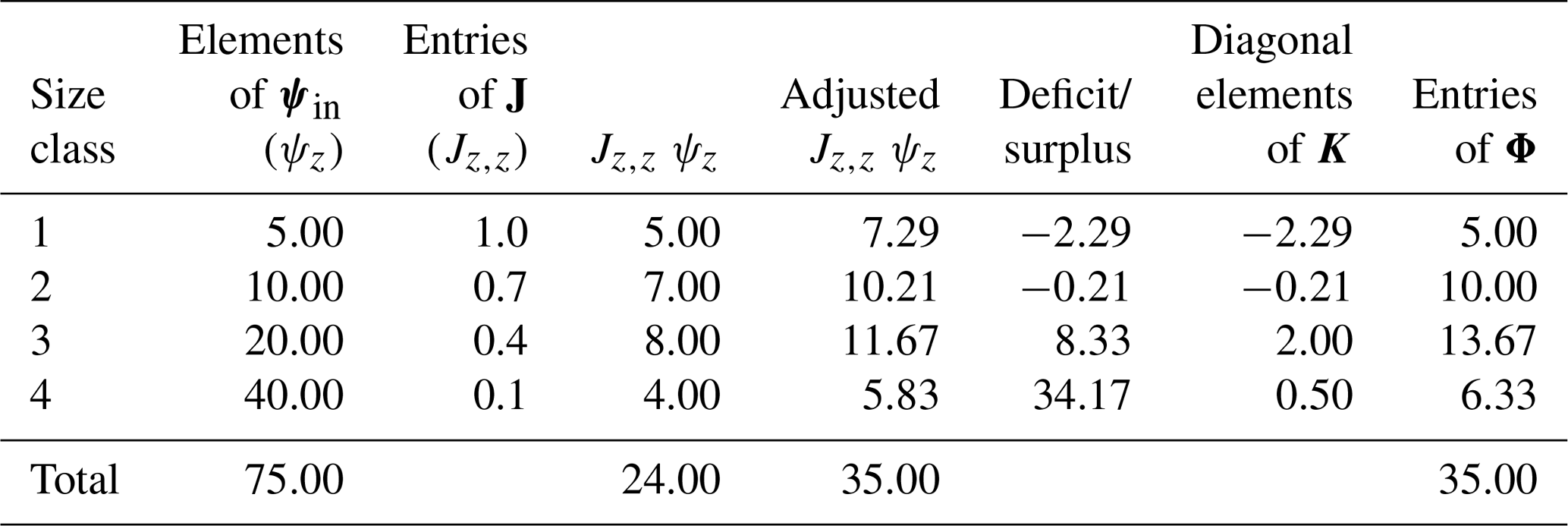
Consider the example values given in Table 2. The total mass of the incoming sediments is 75 kg and the sediments are distributed in four size classes. Here the size class one is the largest and has the highest potential for deposition (with ) while the size class four has the lowest potential for deposition (with ). If the transport capacity Tc is 40 kg, 35 kg of incoming sediments should deposit at the pixel as the total deposition D. Using the value (which is 24) and rescaling these values with D (total deposition mass), we can calculate the masses of sediment which need to be deposited from each grading class. In some cases (when the total deposition D is higher than the value) the mass of material which needs to be deposited can be larger than the available sediments in that particular size class. In this example there is 5 kg of sediments in the first size class and 10 kg of sediments in the second size class respectively. However, our adjusted calculations dictate that there should be a 7.29 kg deposition from the first size class and 10.21 kg from the second size class, which is not possible. So these values needs to be adjusted to reflect the maximum possible deposition from size classes one and two, which are 5 and 10 kg respectively. This adjustment introduces a deficit of 2.5 kg into the total deposition and it needs to be deposited from the third and fourth smaller grading classes. According to the deposition matrix values Jz,z, the deposition probability ratio between the third and fourth grading class is 4:1 (0.4:0.1). The deficit mass, 2.5 kg, is deposited from the third and fourth size class with a 4:1 ratio which accounts for an additional deposition mass of 2 kg from the third size class and 0.5 kg from the fourth size class. In this way the entries of the adjustment vector K are calculated. Depending on the number of size classes and the distribution of the sediments, this adjustment vector K needs to be calculated iteratively.
The deposition of material from the incoming sediment flow reduces the total mass of the sediment load in the flow and changes its distribution due to this size-selective deposition (particles with higher settling velocity deposit faster). The outflow sediment mass vector ψout is then calculated by
Also the deposition height ΔhD is calculated using
The deposition height ΔhD can exceed the surface armour layer thickness (and even the thickness of several soil layers, illustrated in Fig. 2b2 and c2, if the time step is large), and the restructuring of the soil layer grading can be complicated. One solution to this problem is to use a smaller time step. But we preferred to use a conceptualisation that does not impact as much on the numerical efficiency. Details on restructuring the soil column under deposition are given in the following section.
The following section describes the methodology for deriving the deposition transition matrix.
2.3.1 Derivation of deposition transition matrix
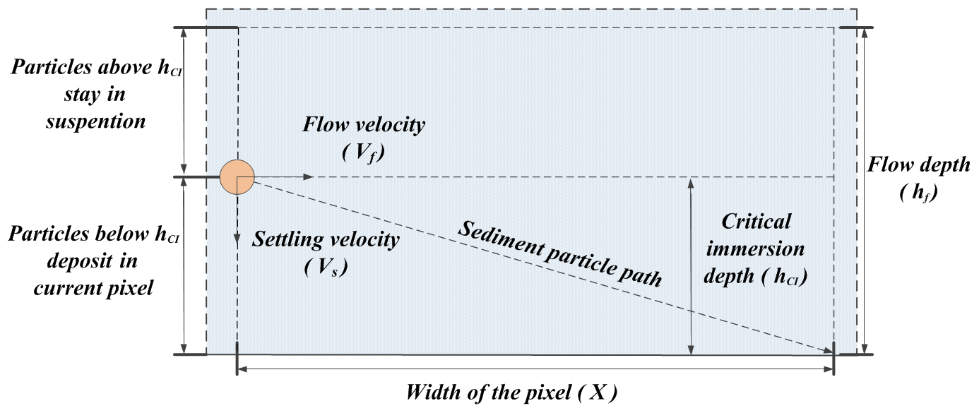
The deposition transition matrix is derived by considering the particle trajectories at the pixel level. Assuming all the sediments flowing into the pixel are homogeneously distributed throughout the water column, we define the critical immersion depth for all the particle size classes as illustrated with Fig. 3. The critical immersion depth is the vertical distance travelled by the particle at the average settling velocity of the particle size class Vz, where it will travel the horizontal distance of the pixel width X under the flow with the fluid flow velocity Vf and settle at the far edge (i.e. exit) of the pixel.
Depending on the position of the sediment particle entering into the pixel with respect to the critical immersion depth, whether or not that particle will deposit in that pixel can be determined. Particles entering the pixel below the critical immersion depth will settle within the current pixel, while particles entering above the critical immersion depth will stay in suspension and exit the current pixel. The critical immersion depth is greater for larger (or denser) particles and less for smaller (or less dense) particles. For sediment particles in larger size classes, the critical immersion depth can be larger than the flow depth Hf (m) (thickness of the water column). That means all the particles in that particle size class will settle in the pixel. Using the critical immersion depth and the flow depth, we can define the diagonal elements Jz,z of the deposition transition matrix J in the following manner.
Note that the deposition transition matrix J is a diagonal matrix which contains only diagonal elements (all off-diagonal elements being 0). The evaluation of elements in the potential deposition matrix J requires the calculation of the critical immersion depth and the flow depth Hf.
The following discussion briefly describes the methodology used to calculate the above variables. The average settling velocity of all the particle size classes can be calculated for typical sediment sizes using Stoke's law (Lerman, 1979).
where ρs and ρf are the bulk density of the soil particles and the density of water (kg m−3) (fluid), g is gravitational acceleration (m s−2), dz is the median particle diameter of the size class z (m), and μ is the dynamic viscosity of water (kg s−1 m−2). The average flow velocity and the flow depth can be calculated using the Manning formula (Meyer-Peter and Müller, 1948; Rickenmann, 1994). Although the Manning formula is normally used to calculate the average flow velocity in channels, we assume that the same formula can be used to calculate the flow velocity at the pixel level assuming water flowing over a pixel as a small channel segment. The Manning formula states
where n is the Manning roughness coefficient, R is the hydraulic radius (m), and S is the slope (m m−1). The Manning roughness coefficient n can be approximated using the median diameter d50 (mm) of the surface armour layer (Coon, 1998) using following equation.
The hydraulic radius is the ratio between the cross-sectional area of the flow and the wetted perimeter. When we consider the flowing water column at a pixel, the cross-sectional area of the flow is the multiplication of flow width (pixel width) ω and the flow depth Hf, with the wetted parameter being the flow width ω. The hydraulic radius at the pixel is then the flow depth Hf. Substituting flow depth for hydraulic radius Eq. (11) becomes
The flow velocity at the pixel can be also expressed in terms of upslope contributing area Ac, runoff excess generation r, flow width ω, and flow depth Hf.
Solving the Eqs. (13) and (14) the flow depth Hf and the flow velocity Vf can be calculated in terms of Ac, r, ω, S, and n using
2.3.2 Restructuring of the soil layers after deposition
Deposition of sediment on the soil surface moves the soil surface upwards (soil model space moves upwards). As mentioned earlier the deposition height ΔhD can exceed the surface armour layer thickness and/or a number of subsurface soil layer thicknesses. Figure 2b2 illustrates a typical scenario where the deposition height has exceeded the thickness of the surface armour layer Dsur.
Figure 2b2 and c2 show the movement of the model space for three soil layers. In the restructured soil column (Fig. 2c2) the new third layer consists of a portion of the original layer one (surface armour layer) and the first original subsurface layer. Because of the upward movement of the model space, a portion of the second original soil layer and the entire third soil layer has been incorporated into the new bedrock layer. However, the grading of the new bedrock layer remains unchanged although the material from the original soil layers two and three is added to the bedrock layer. At the first glance it may seem that this process would drastically alter the soilscape evolution dynamics by introducing a sharp contrast in soil grading at the soil–bedrock interface. In SSSPAM a large number of soil layers (50 to 100) are used to ensure smooth soil grading transition from soil to bedrock.
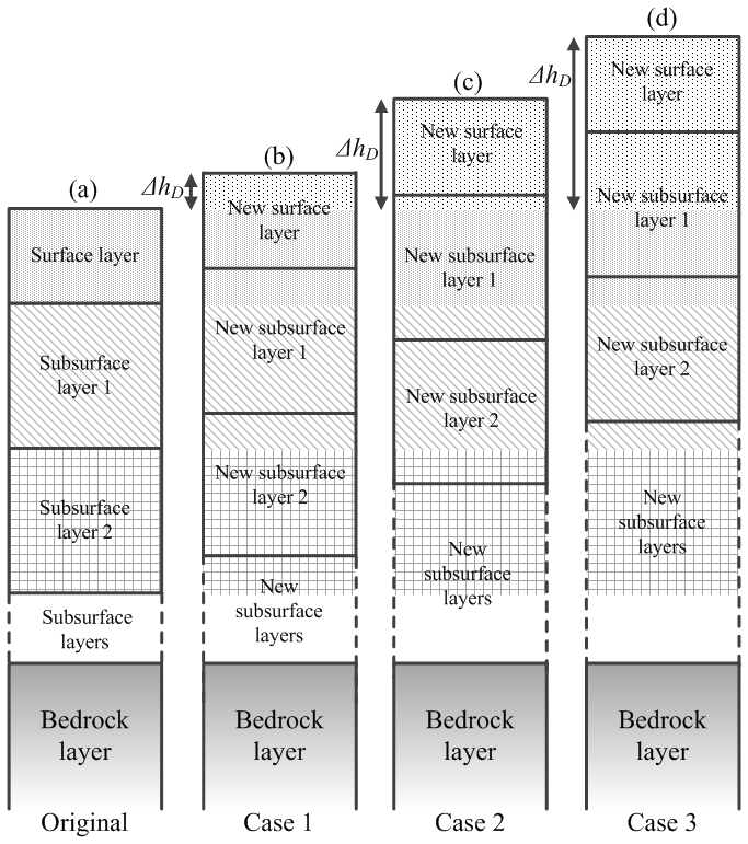
Figure 4 shows three different cases that can occur during the deposition process. In Case 1 (Fig. 4b) the deposition height ΔhD is less than the surface armour thickness Dsur. In Case 2 (Fig. 4c) the deposition height ΔhD is greater than the surface armour layer thickness Dsur, and the original surface armour layer is situated inside a single new subsurface layer. Also the new soil subsurface layer which contains the original surface armour layer can reside in any depth within the new soil profile depending on the deposition height (e.g. it can be the first, second, fifth, or any subsurface layer). For simplicity of explanation, Fig. 4c shows this layer in the first new subsurface layer. Case 3 (Fig. 4d) is similar to the situation in Case 2 where the deposition height ΔhD is greater than the surface armour layer thickness Dsur. However, in this case the original surface armour layer belongs to two new subsurface layers instead of one. As with Case 2, the new soil subsurface layers, which contain portions of the original surface armour layer, can reside at any depth within the new soil profile. Calculation of soil grading of the surface and all the subsurface soil layers is performed with different approaches according to the previously mentioned deposition scenarios. A detailed description of these soil grading approaches can be found in Welivitiya (2017).
2.4 Soil profile weathering
The methodology used for simulating weathering within the soil profile is detailed by Welivitiya et al. (2016). It uses a physical fragmentation mechanism where a parent particle disintegrates into n number of daughter particles with a single daughter particle retaining fraction α of the parent particle by volume and the remaining n−1 daughter particles retaining fraction 1−α of the parent particle volume. By changing n and α we can simulate a wide range of particle disintegration geometries which can be attributed to different weathering mechanisms. In this paper we used n=2 and α=0.5 to simulate symmetric fragmentation mechanism where a single parent particle breaks down into two equal daughter particles. But the model can simulate any values of n and α which can simulate a wide range of weathering mechanisms ranging from symmetric fragmentation to granular disintegration. We decided to use the symmetric fragmentation mechanism based on the results of Wells et al. (2006). Using the above-mentioned parameters, parent–daughter particle diameters, and soil grading distribution values, the weathering transition matrix is constructed according to the methodology described by Cohen et al. (2009) and will not be discussed further.
The weathering rate of each soil layer is simulated using a depth-dependent weathering function. It defines the weathering rate as a function of the soil depth relative to the soil surface depending on the mode of weathering of that particular material. SSSPAM can use different depth-dependent weathering functions to simulate the soil profile weathering rate. For the initial simulations presented in this paper we used the exponential (Humphreys and Wilkinson, 2007) and humped exponential (Ahnert, 1977; Minasny and McBratney, 2006) depth-dependent weathering functions. A detailed explanation and the rationale of these weathering functions are presented in Welivitiya et al. (2016) and extended by Willgoose (2018).
It is important to note that SSSPAM can assign different weathering mechanisms (using different values of n and α) and different depth-dependent weathering functions for each pixel (node) depending on the material and the dominant weathering drivers (such as temperature) in the pixels' geographical location. Also, if need be, the depth-dependent weathering function at each pixel may be changed during the simulation to reflect any perceived temporal change in weathering drivers by slightly modifying the weathering module. This will allow SSSPAM to conduct simulation studies on global change incorporating both physical and chemical weathering processes on soilscapes in the future.
The objective of the simulations below was to explore the capabilities and implications of the SSSPAM coupled soilscape–landform evolution model. Although the model is capable of simulating soilscape and landform evolution for a three-dimensional catchment-scale landform, a synthetic two-dimensional linear hillslope (length and depth) landform was used here. Because it is two-dimensional, the landform always discharges in a single direction. In this way the complexities of multidirectional discharge were avoided so we can focus on the soilscape–landform coupling.
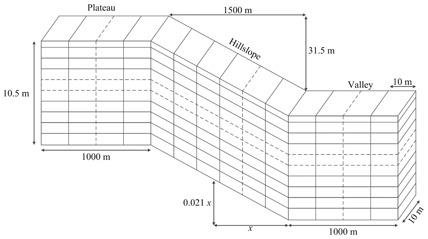
The simulated landform starts from an almost flat 1 km long plateau (almost flat area at the top of the hillslope) with a very small gradient of 0.001 % (Fig. 5). A hillslope with a gradient of 2.1 % starts at the edge of the plateau and continues 1.5 km horizontally while dropping 31.5 m vertically and terminates at a valley. The valley (another almost flat area at the bottom of the hillslope) itself has the same gradient as the upslope plateau (0.001 %) and continues for another 1 km. The valley (the bottom section of the landform) is designed to facilitate sediment deposition so the effect of sediment deposition on soilscape development can be analysed. The simulated hillslope has a constant width of 10 m (one pixel wide) and is divided into 350 10 m long pixels along slope. At each pixel the soil profile is defined by a maximum of 102 soil layers. The soil surface armour layer is the topmost soil layer and it has a thickness of 50 mm. The 100 layers below the surface layer are subsurface soil layers with a thickness of 100 mm each. The bottommost layer (102nd layer) is a permanent non-weathering layer and it is the limit of the hillslope modelling depth. In this way SSSPAM is capable of modelling a soil profile with a maximum thickness of 10.05 m. By changing the number of soil layers used in the simulation SSSPAM is able to simulate a soil profile with any thickness. However, as the number of model layers increases, the time required for the each simulation also increases. During our initial testing, we found that the soil depth rarely increased beyond 10 m and decided to set 10.05 m as the maximum soil depth for this scenario.
Two soil grading data sets (Table 3) were used for the initial surface soil grading and the bedrock. The first soil grading was from Ranger Uranium Mine (Northern Territory, Australia) spoil site. This soil grading was first used by Willgoose and Riley (1998) for their landform simulations. It was also subsequently used by Sharmeen and Willgoose (2007) for their work with ARMOUR simulations and Cohen et al. (2009) for mARM simulation work. The soil grading consisted of stony metamorphic rocks produced by mechanical weathering with a body fracture mechanism (Wells et al., 2008). It had a median diameter of 3.5 mm and a maximum diameter of 19 mm (Table 3 – Ranger1a). The second grading was created to represent the bedrock of the previous soil grading. It contained 100 % of its mass in the largest particle size class that is 19 mm (Table 3 – Ranger1b). These soil gradings are the same soil gradings used in the SSSPAM parametric study of Welivitiya et al. (2016). At the start of the simulation the surface armour layer was set to the soil grading (Table 3 – Ranger1a) and all the subsurface layers were set to bedrock grading (Table 3 – Ranger1b). The discharge (runoff excess generation) rate of water is derived from averaging the 30-year rainfall data collected by Willgoose and Riley (1998). Using the simulation setup described above, simulations were carried out using the yearly averaged discharge rate. For this simulation we set the time step to 10 years and the model was run for 10 000 time steps (simulating 100 000 years of evolution).
Table 3Soil grading distribution data used for SSSPAM simulation.
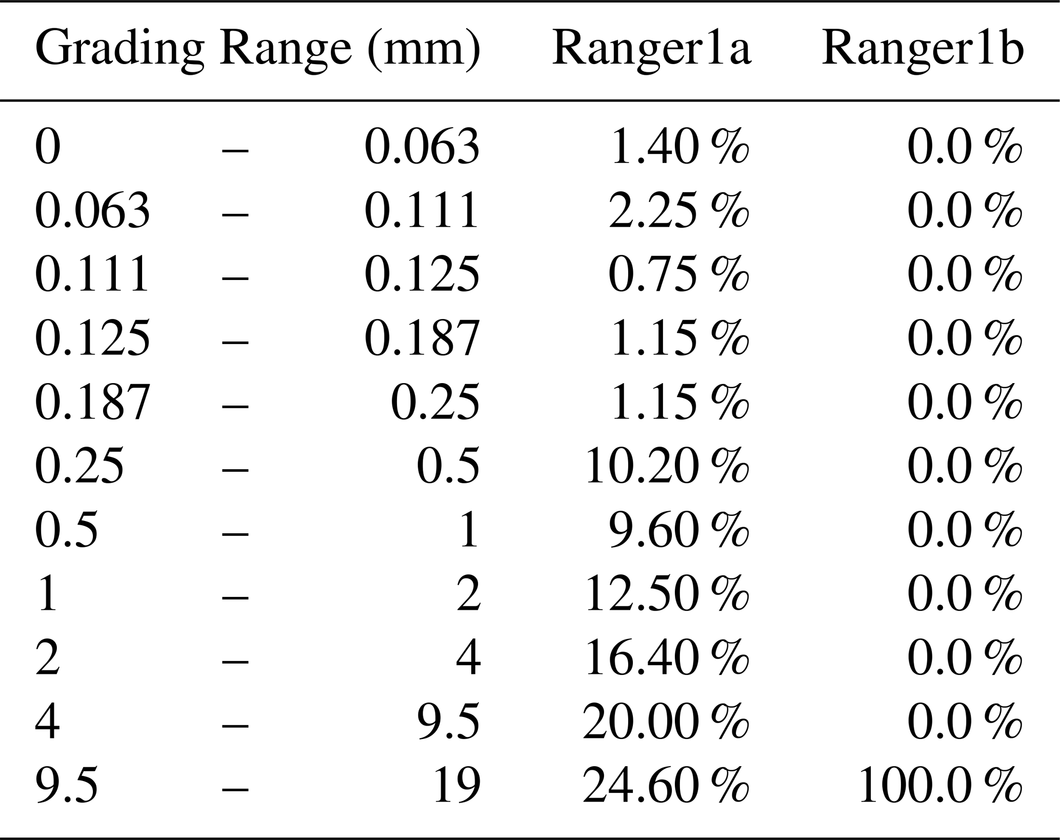
Figure 6 shows six outputs at different times during hillslope and soil profile evolution.
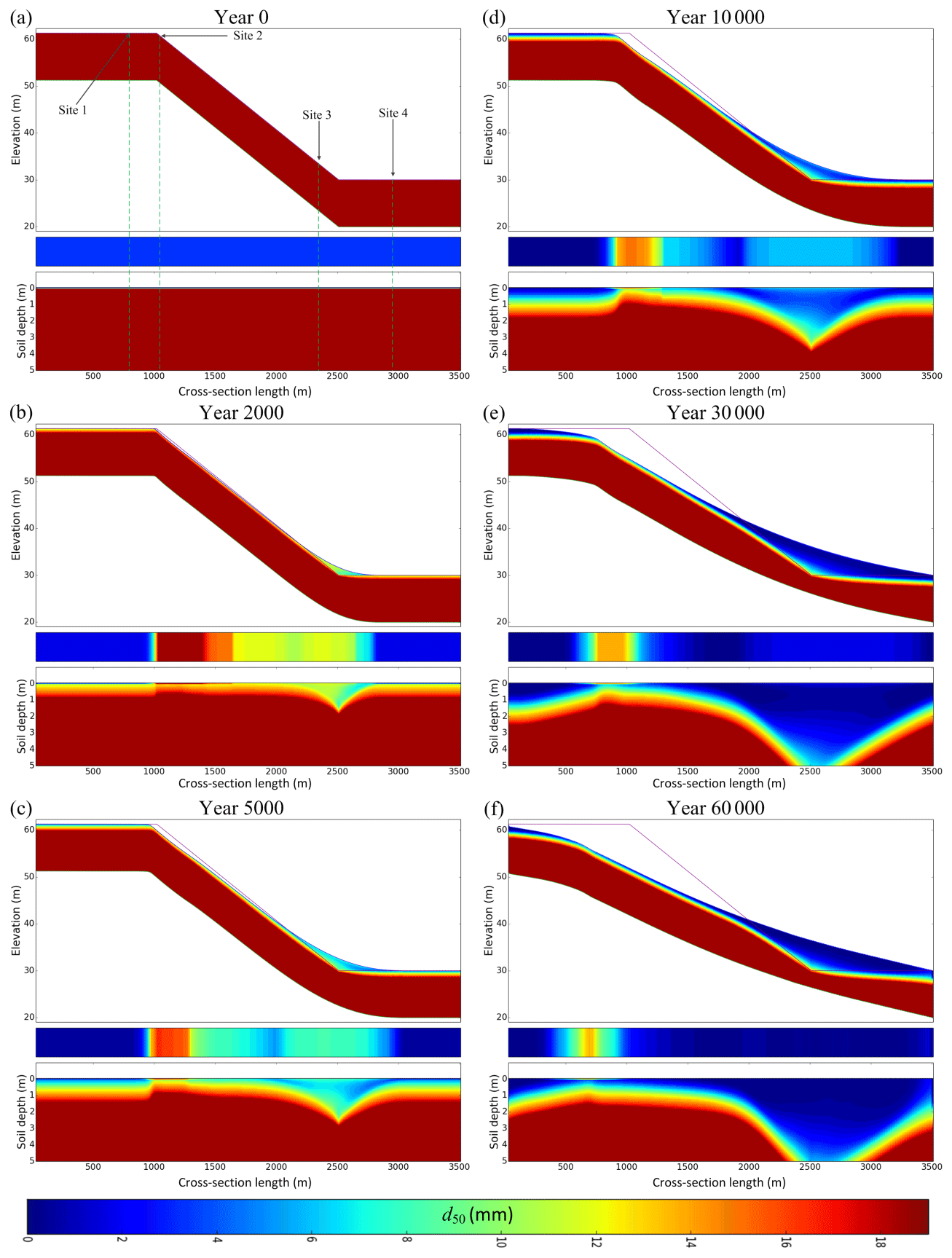
Figure 6Evolution of the soilscape with the exponential depth-dependent weathering function.
The upper section in each of the panels in Fig. 6 is the cross-section median diameter (d50) of the soil profile and the landform, with the line denoting the original landform surface. The middle panel is the median diameter d50 of the soil surface armour layer. The bottom panel is the soil profile relative to the surface highlighting the soil profile d50 (i.e elevation differences at different nodes are removed and the d50 for all the nodes are displayed at the same level). The soil depth is the depth below the surface at which d50 reaches the maximum possible particle size (i.e. the bedrock grading). Figure 6a shows the initial condition for the soilscape: a deep bedrock overlain by a very thin fine-grained soil layer. The evolution of the coupled soilscape and landform at different simulation times is presented in Fig. 6b–f.
If we initially consider the landform evolution alone, the erosion-dominated regions and the deposition-dominated regions can be clearly identified. Initially erosion is highest on top of the hillslope where the plateau transitions to the hillslope (plateau–hillslope boundary) and erosion gradually reduces down the hillslope. Also, there is a sharp increase in surface d50 at the plateau–hillslope boundary and then a gradual decrease down the hillslope. The summit plateau has a very low slope gradient, and although the contributing area increases across the plateau, the potential erosion and the transport capacity of the flow remains negligible, resulting in minimum erosion. At the plateau–hillslope boundary, the slope gradient suddenly increases. This increase in slope gradient and high contributing area increases the potential erosion of the flow and causes a rapid increase in transport capacity downslope. This erosion gradually reduces further down the hillslope despite increasing contributing area. Although the transport capacity increases towards the bottom of the hillslope, water flowing over the downslope nodes is laden with sediments already eroded from upslope nodes. This reduces the amount of erosion at the downslope nodes.
Turning to the evolution of the soil profile, the upslope plateau retains the initial surface soil layer without any armouring due to the very low erosion, and it develops a relatively thick soil profile as a result of bedrock weathering. The high erosion rate at the plateau–hillslope boundary removes all the fine particles from the initial soil layer as well as fine particles produced by the weathering process, creating a very coarse surface armour layer. This high erosion rate also leads to a relatively shallow soil profile. The erosion rate reduces down the slope due to saturation of the flow with sediments from upstream. Low erosion leads to a weak armouring, and the fine particles produced from surface weathering remain on the surface. These processes lead to the fining of the surface soil layer and thickening of the soil profile down the hillslope.
With time the location of the high erosion region shifts upstream onto the plateau cutting into it. The d50 of the armour layer downslope also decreases. Both of these changes occur due to lowering of the slope gradient of the hillslope over time.
Deposition of material occurs on either side of the hillslope–valley boundary. The valley at the foot of the hillslope has a very low initial slope gradient. At the hillslope–valley boundary (toe slope) the slope gradient reduces suddenly. This sudden slope gradient reduction reduces the transport capacity of the water flow and initiates deposition. Initially deposition occurs only at the hillslope–valley boundary node and increases its elevation. This deposition and slope reduction propagates upslope until equilibrium is reached with erosion. Deposition propagates across the valley and produces the deposits in Fig. 6.
There is a change in surface d50 between the erosion and deposition regions starting at around 2000 m. The surface d50 of the erosion region reduces down the slope, reaches a minimum at 2000 m, and then increases as it transitions into the deposition region. This can be clearly seen in Fig. 6c and d. As noted previously, the actual erosion rate reduces down the slope due to saturation of the flow with sediments. At the end of the erosion region no more erosion can take place because the flow is completely saturated with sediment. Because of the lack of erosion, fine particles are not removed from the surface and weathering produces more and more fine particles, reducing the surface d50 and increasing the soil depth.
Near the erosion–deposition boundary, only a small amount of sediment is deposited. Since the larger particles have the highest probability of deposition, a small amount of coarse material deposits there. Downslope into the deposition region the slope further decreases, the difference between the transport capacity and the sediment load increases, and the rate of deposition steadily increases. Since larger particles have a higher probability of depositing first, coarse material preferentially deposits. Mixing of these coarse particles with pre-existing weathered fine particles produces the observed coarsening of the surface d50. Once the surface d50 of the deposition region reaches a peak, it starts to decrease again (from 2500 to 3000 m). Beyond 3000 m the deposited material is smaller because the larger particles have already been deposited upstream. The deposition of each consecutive downstream node consists of finer particles leading to the observed decrease in surface and profile d50. As expected the soil thickness is higher in the deposition regions than the other regions.
With time the deposition region moves upslope. The gradient of d50 observed in earlier times of the deposition region (until 30 000 years) decreases, and the soil changes into a very fine-grained homogeneous material resulting from surface weathering. Due to the high weathering rate at the surface and the upper soil layers, the deposited sediment decomposes into a very fine material. With time, the d50 of the sediments in the water flow also decreases due to low erosion potential and weathering of the surface armour layer of upslope nodes. For these reasons the d50 of the deposition region decreases and becomes homogeneous, leading to burial of the coarse material that was deposited earlier.
The simulation produced a landform morphology which resembles the five-unit model proposed by Ruhe and Walker (1968). At the conclusion of the simulation the plateau area resembles a flat summit, the plateau–hillslope boundary resembles the convex shoulder, the transition region from the plateau–hillslope boundary to the deposition region resembles the backslope with a uniform slope, and the deposition region resembles the concave base divided into upper footslope and lower toeslope. Generally the soil grading distribution is fine at the summit and coarsens from the summit to the shoulder and backslope followed by fining from the backslope to the base (Birkeland, 1984). Furthermore, the soil depth is typically high in the summit area, low in the shoulder and backslope, and high in the upper footslope and lower toeslope (Brunner et al., 2004). The soil grading and the soil depth variations of our simulations produce similar trends.
Evolution characteristics of different sites
In order to better understand the dynamics of soilscape evolution we also plotted the elevation, slope, rate of erosion (and/or deposition), surface d50, soil depth, and profile d50 for four sites (Fig. 6a). The first two sites (sites 1 and 2) are on either side of the plateau–hillslope boundary in the erosion region. The other two sites (sites 3 and 4) are on either side of the hillslope–valley boundary in the deposition region.
4.0.1 Site 1 and 2
For site 1 (Fig. 7 – solid line plots) the erosion and surface d50 are strongly correlated over time. The soil depth and profile d50 plots are also highly correlated. The abrupt change in profile d50 occurs at the same time as abrupt changes in soil depth. Site 1 initially has small erosion because the slope is very low. This small amount of erosion means the elevation and slope are initially constant. Due to the dominance of weathering, both surface and profile grading become enriched with fine particles and the d50 decreases. Weathering of the profile layers creates a relatively deep soil profile. With time the erosion front, initially at the plateau–hillslope transition, cuts back into the plateau. The increased erosion rate removes the fine material created by weathering, leading to a coarse-grained armour. This observation may have some important implications for the landform evolution modelling community. Most landform evolution models which do not explicitly model soil profile evolution or weathering consider a single unchanging soil layer on top of the landform. When evolving a landform similar to the setup used in this paper, such landform evolution models may underestimate the upward propagation rate of the erosion front as they will be trying to erode relatively coarser particles. With weathering producing smaller particles, the erosion front would propagate faster in a natural hillslope.
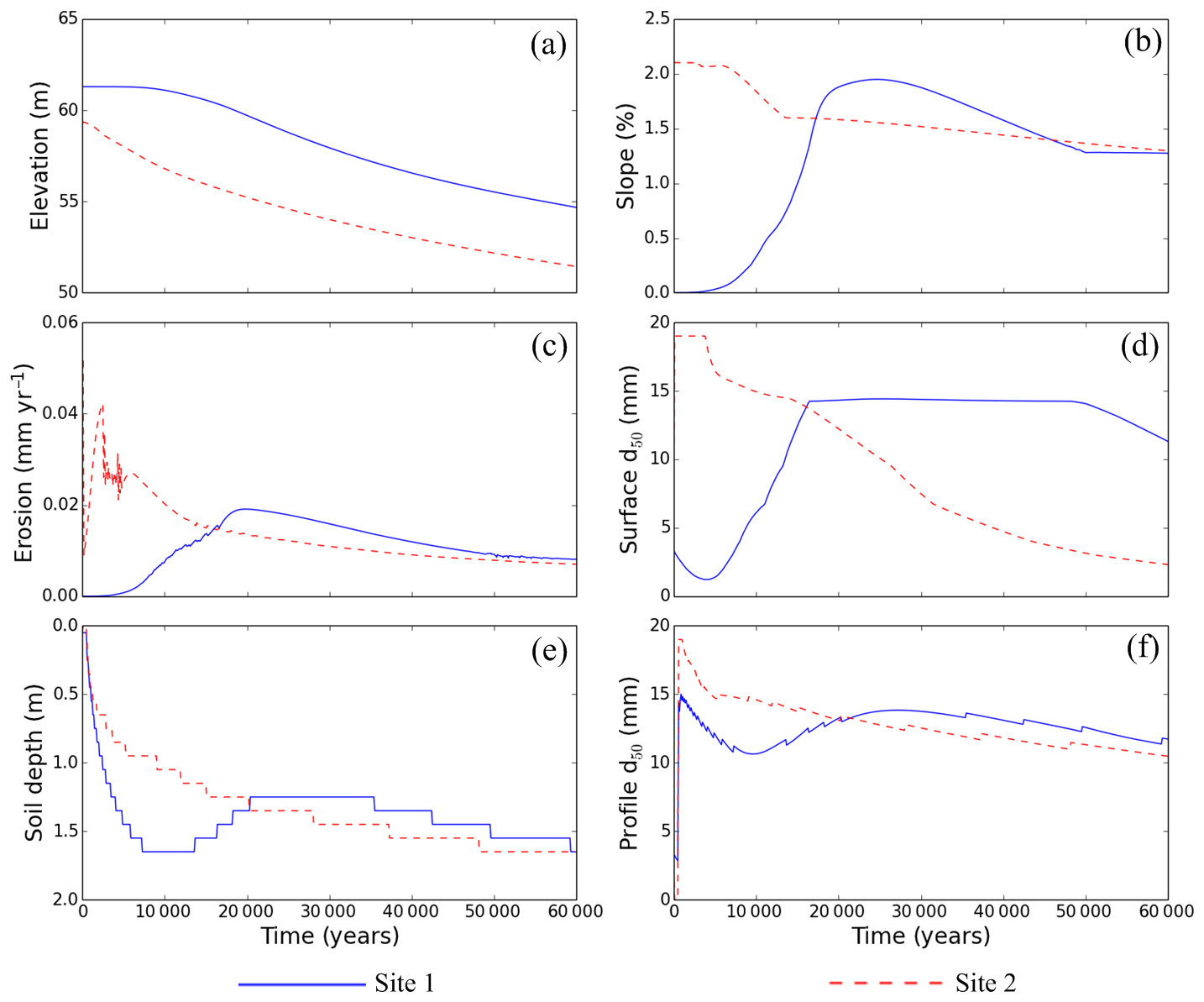
Figure 7Evolution characteristics of sites 1 and 2: (a) elevation, (b) hillslope gradient, (c) erosion rate, (d) surface d50, (e) soil depth, and (f) profile d50.
When the erosion front crosses site 1, the gradient increases as does the erosion rate (at around 20 000 years). During this phase of increasing erosion the surface d50 also increased. However, the surface d50 stabilises around 14 mm before the erosion rate reaches its maximum value. This is because once total armouring occurs, the erosion is reduced to a very low value. Although the erosion is low, the slope of the site 1 continues to increase until it reaches a maximum and the Shields shear stress threshold diameter also increases. This allows erosion to keep increasing while the surface d50 remains essentially constant. When the erosion rate overtakes the rate of production of weathering, the soil depth decreases. Increasing erosion reduces the soil thickness while coarsening the surface of upper soil layers. This results in the increase in the profile d50 at later times. At 20 000 years, the reduction of slope reduces the rate of erosion so that weathering again dominates the site. Weathering produces more fine particles reducing the surface d50 from about 48 000 years. The dominance of weathering over erosion also increases the soil depth while decreasing the profile d50.
Both soil depth and profile d50 plots resemble a stair-stepped graph. The reason for this appearance is that SSSPAM calculates soil depths as the number of soil profile layers. The model does not interpolate the depth of soil within a single layer. Since the profile d50 is a function the soil thickness, this plot also displays this pattern.
For site 2 (Fig. 7 – dashed line plots) the evolution is simpler than site 1. The initial transport capacity and discharge energy at site 2 is very high while the sediment inflow from upstream is low because of low erosion from the plateau. The resulting higher erosion rate produces a very coarse surface layer and exposes the bedrock in the subsurface. This effect causes both the surface d50 and profile d50 to rapidly increase to the maximum possible diameter (bedrock grading).
Although the surface d50 has reached the maximum possible diameter the erosion continues to increase as the Shields threshold diameter for entrainment of the water flow has increased beyond the maximum particle size (19 mm) and the bedrock grading itself is being eroded. However, at around 2700 years the Shields threshold diameter decreases below 19 mm, and the fully armoured surface causes the erosion rate to decrease rapidly and becomes unstable in time with rapid fluctuations. Once an armour layer develops on the surface, the profile layers are protected from erosion and weathering becomes more dominant, so the profile d50 decreases while soil depth increases.
4.0.2 Site 3 and 4
For site 3 (Fig. 8 – solid line plots) the elevation increases due to deposition. The initial increase in surface d50 occurs due to size-selective deposition. As noted in the model description, larger particles deposit at a higher rate. This deposition of larger particles on the surface causes the surface d50 to initially increase.

Figure 8Evolution (near the hillslope–valley boundary) of sites 3 and 4: (a) elevation, (b) hillslope gradient, (c) erosion rate, (d) surface d50, (e) soil depth, and (f) profile d50.
The subsequent decrease in the surface d50 occurs due to a combination of two processes. Firstly, with time the upstream boundary of the deposition region moves upslope, and since the largest particles tend to deposit at the beginning of the deposition region, the sediment flow at site 3 gets enriched with more and more fine particles. Due to the deposition of these relatively finer particles the surface d50 tends to decrease. Secondly, weathering of the surface and the subsurface layers reduces the surface d50. Compared to sites 1 and 2 the soil depth increase of site 3 is much higher. In sites 1 and 2 the soil profile growth only occurred due to the excess of weathering over erosion. At site 3 the soil layer grows due to material deposition as well as weathering of the bedrock. The profile d50 increases in the initial stage.
For site 4 (Fig. 8 – dashed line plots), while the initial evolution is different, in the latter stages (beyond year 15 000) the evolution characteristics of the soil properties are similar to those of site 3. Since the valley initially has a low slope, the initial erosion is negligible and the elevation, slope, and erosion remain close to 0. With the growth of the deposition region, a deposition front moves across the valley. Before the deposition front reaches site 4, the elevation, slope, and erosion/deposition remain unchanged. Because the initial erosion rate at site 4 is low, there is no armouring so that weathering dominates and the surface d50 decreases. When the deposition front reaches site 4, the elevation increases due to sediment deposition and so does the slope. Due to the size-selective deposition of coarse sediment the surface d50 increases. Afterwards the evolution of the soil properties is similar to site 3 as the same processes are acting at sites 3 and 4.
To test the sensitivity of the conclusions in the previous section to changes in the depth-dependent weathering functions, in this section we explore the effect of weathering using the humped exponential weathering function. The key difference is that the humped function has a low weathering rate at the surface with the peak weathering rate occurring mid-profile.
Superficially, both the humped and exponential weathering functions produce similar trends; however, there are some differences in the particle size distribution, soil depth, and the evolution of the landform (Fig. 9). At identical times the surface d50 is coarser and the soil depth is less for the humped simulations. There is also a subtle difference in the initial landform evolution. For the exponential weathering function the highest erosion rate occurs near the plateau–hillslope boundary (year 2000 near 1000 m, Fig. 6). For the humped function this maximum soil surface deviation occurs further down the hillslope (year 2000 near 1500 m, Fig. 9). For subsequent times, this difference in the location of the maximum erosion leads to subtly different landforms.
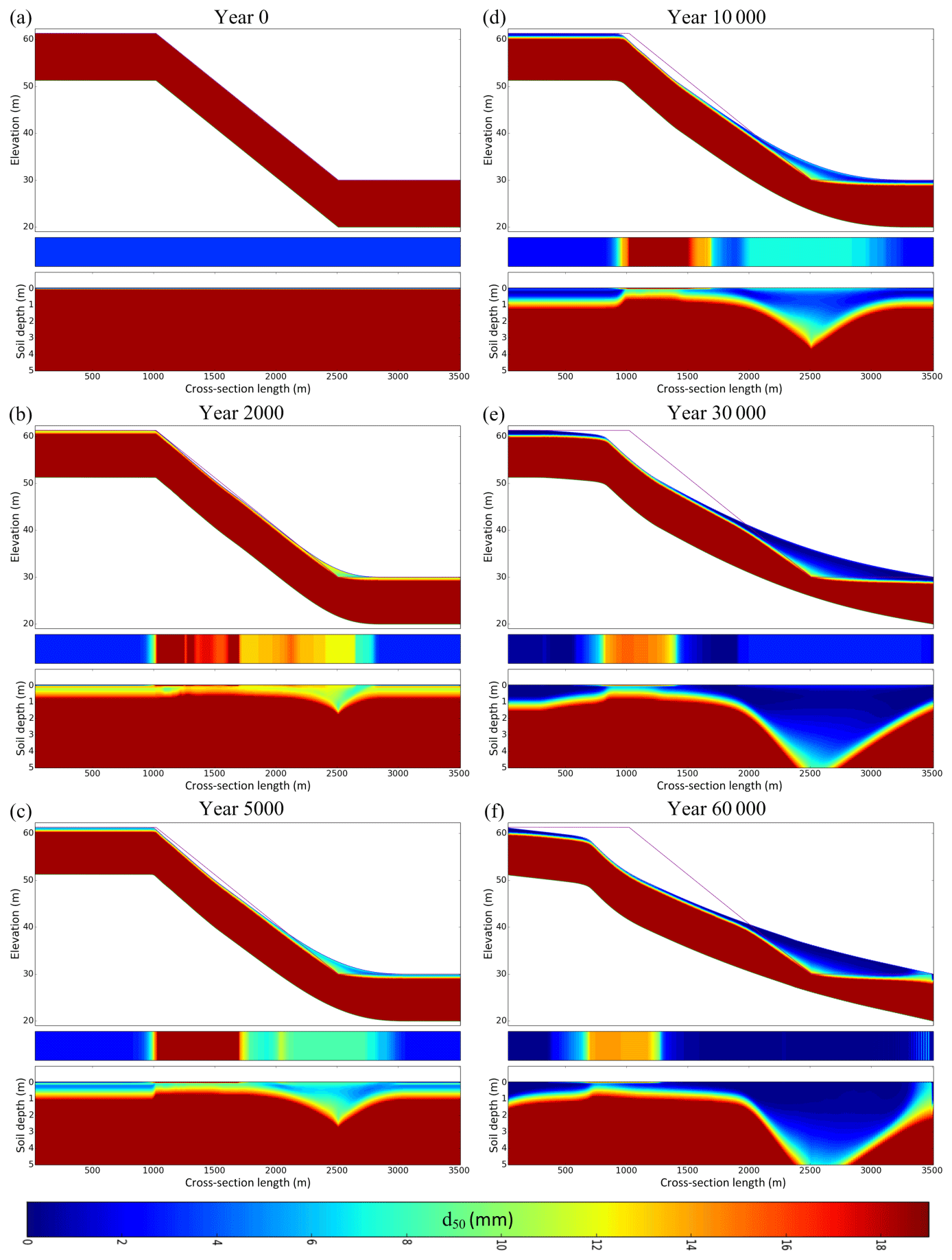
Figure 9Evolution of the soilscape with the humped exponential depth-dependent weathering function.
These differences in landform evolution are explained by the near surface weathering rates. For the exponential weathering function the weathering rate is highest at the surface and declines exponentially with depth. For the humped exponential weathering function the highest weathering rate is at a finite depth below the surface and exponentially decreases below and above this depth. Because of the lower surface weathering rate for humped, the surface d50 remains coarser during the entire simulation. The relative coarseness of the surface means that the water flow needs to be more energetic to entrain material from the surface due to the Shields stress entrainment threshold. For the exponential weathering function simulations, shear stress of the water flow is high enough to entrain most of the surface soil particles near the plateau–hillslope boundary owing to the finer armour layer as a result of surface weathering. However, for the humped exponential weathering simulations the surface armour is coarser because of the lower surface weathering rate, and the shear stress of the water flow is not high enough to detach material from the armour layer. Because of this, the highest erosion occurs downslope where the contributing area is higher and hence the shear stress of the water flow is higher.
Currently the coupled soilscape–landform evolution model SSSPAM presented here is limited in its scientific scope. The model is based on physical fragmentation of parent soil particles, and it does not model chemical transformations. Also at the current time SSSPAM does not account for soil organic carbon (SOC) and its influence in the soil formation and evolution processes. The modelling approach used here is complimentary to the chemical weathering modelling work done by Kirkby (Kirkby, 1977, 1985, 2018). However, we will be incorporating a physically based chemical weathering model described by Willgoose (2018) into SSSPAM in the future. All available evidence suggests that, in order to effectively model SOC, it will require an extremely complicated coupled model which requires soil grading, soil moisture, and vegetation and decomposition rates. Although formulating such a model is very desirable (and would be an important endeavour by itself) for the entire scientific community, it is well beyond the scope of this current research work.
The deposition model of SSSPAM is designed in such a way that the difference between the transport capacity and the sediment load of the flow is always deposited regardless of the settling velocities. This is done to prevent the flow from being over the transport capacity. Depending on the material grading distribution and the concentration in the profile of the flow, the theoretical amount of the material that can be deposited can be different. In this model formulation we assume that the sediment grading is uniform and the sediment concentration is also uniform within the flow. The reality may not be as simple as that. There is some literature such as Agrawal et al. (2012) which argues that the sediment concentration profile has an exponential distribution (i.e. most of the sediments are concentrated near the bottom of the flow) and that the grading distribution profile in the flow is also a function of the settling velocity of different particles (i.e. larger particles are concentrated near the bottom of the flow). So in practice the amount of material deposited at each pixel according to the critical immersion depth might be higher. Although the approach used in SSSPAM may not perfectly mimic the natural behaviour of sediment deposition, we believe that this is an effective way to numerically represent this process in the model at this time.
The main objective of this paper was to introduce the new coupled soilscape–landform evolution model. Here some applications of the model simulations albeit simple were presented to show how the model performed in reality and to highlight some of the geomorphic signatures emerging from the modelling results itself. The simulation setup may not be a reasonable application that necessarily reflects the total environment. However, we are inspired by the early work on hillslope geomorphology by authors such as Kirkby (1971) and Carson and Kirkby (1972) which was very useful in understanding hillslope evolution processes. So as a first step we used a one-dimensional hillslope to run our simulations because understanding dynamics of 1-D hillslope evolution is simpler and we can better illustrate possible implications for different processes. Further, only limited comparison with field data was possible because of a dearth of any experimental work done by other researchers using setups comparable with our simulations. However, a subsequent paper will deal with implications of model results in terms of one-dimensional and three-dimensional alluvial fans. In this paper, we compare and contrast the model results with experimental work done by authors like Seal et al. (1997) and Toro-Escobar et al. (2000), as well as general observations on naturally occurring alluvial fans and their formation dynamics.
This study presents a methodology for incorporating landform evolution into the SSSPAM soil grading evolution model. This was achieved by incorporating elevation changes produced by erosion and deposition. Previous published work with SSSPAM assumed that the landform, slope gradients, and contributing areas remained constant during the simulation. This did not preclude the landform from evolving, only that the soil reached equilibrium faster (i.e. had a shorter response time) than the landform evolved (i.e. a “fast” soil, Willgoose, 2018). In the new version of SSSPAM discussed here, the elevations, contributing area, slope gradient, and slope directions at each node dynamically evolve. This new model explicitly models co-evolution of the soil and the landform, where the response times for soil and landform are similar.
By defining the critical immersion depth, a novel and simple methodology for size-selective deposition was introduced to formulate the deposition transition matrix. This deposition transition matrix characterises the size selectivity of sediment deposition depending on the settling velocity of the sediment particle, with faster settling velocity particles settling first.
The results demonstrated SSSPAM's ability to simulate erosion, deposition, and weathering processes which govern soil formation and its evolution coupled with an evolving landform. The simulation results qualitatively agree with general trends in soil catena observed in the field. The model predicts the development of a thin and coarse-grained soil profile on the upper eroding hillslope and a thick and fine-grained soil profile at the bottom valley. Considering the dominant process acting upon the soilscape, the hillslope can be divided into weathering-dominated, erosion-dominated, and deposition-dominated sections. The plateau (summit) was mainly weathering-dominated due to its very low slope gradient and low erosion rate. The upper part of the hillslope was erosion-dominated owing to its high slope gradient and high contributing area. The lower part of the hillslope and the valley was deposition-dominated. The position and the size of these sections change with time due to the evolution of the landform and the soil profile. During the simulation, the weathering-dominated region shrinks due to the erosional region dominating it. The erosion-dominated region expands upslope into the previously weathering-dominated region, and the downstream boundary retreats upslope away from the deposition-dominated region but shows a net expansion in area. The deposition-dominated region expands upslope into the previously erosion-dominated region with a net expansion.
The simulation results also show how the interaction of different processes can have unexpected outcomes in terms of soilscape evolution. The best example is the fining of the surface grading despite an increasing transport capacity and potential erosion rate. This occurs due to saturation of the flow with sediment eroded from upstream nodes. Further, the comparison of results produced by the exponential and humped exponential weathering functions showed how the distribution of weathering rate down the soil profile changes the overall properties of the soilscape. For instance, the humped exponential simulation produced a thinner soil profile and coarser soil surface armour compared with simulation results of exponential weathering function because of the reduced weathering rate at the soil surface. This led to a longer-lived surface armour for the humped function.
The synthetic landform simulations demonstrated SSSPAM's ability to qualitatively simulate erosion, deposition, and weathering processes and to generate familiar soilscapes observed in the field. Comparison of results obtained from two different depth functions demonstrates how the soilscape dynamic evolution is influenced by the weathering mechanisms. This in turn links to the geology of the soil parent materials and their preferred weathering mechanism, which leads to the heterogeneity of soilscape properties in a region. A future paper will discuss how this work can be extended to include the impact of chemical weathering into soilscape evolution.
The SSSPAM model (computer code, parameters) and data (soil grading and elevation data) used in this paper are available on request from the authors.
The authors declare that they have no conflict of interest.
The authors would like to acknowledge Peter Finke and Arnaud Temme for their review comments which greatly assisted in strengthening this paper. The research work presented in this paper were performed while the lead author was on a post graduate scholarship from The University of Newcastle, Australia.
This research has been supported by the Australian Research Council (grant no. DP110101216).
This paper was edited by Andreas Baas and reviewed by Arnaud Temme and Peter Finke.
Agrawal, Y. C., Mikkelsen, O. A., and Pottsmith, H.: Grain size distribution and sediment flux structure in a river profile, measured with a LISST-SL Instrument, Sequoia Scientific, Inc. Report, 2012.
Ahnert, F.: Some comments on the quantitative formulation of geomorphological processes in a theoretical model, Earth Surf. Process., 2, 191–201, https://doi.org/10.1002/esp.3290020211, 1977.
Arya, L. M. and Paris, J. F.: A physicoempirical model to predict the soil moisture characteristic from particle-size distribution and bulk density data, Soil Sci. Soc. Am. J., 45, 1023–1030, 1981.
Behrens, T. and Scholten, T.: Digital soil mapping in Germany – a review, J. Plant Nut. Soil Sci., 169, 434–443, https://doi.org/10.1002/jpln.200521962, 2006.
Benites, V. M., Machado, P. L. O. A., Fidalgo, E. C. C., Coelho, M. R., and Madari, B. E.: Pedotransfer functions for estimating soil bulk density from existing soil survey reports in Brazil, Geoderma, 139, 90–97, https://doi.org/10.1016/j.geoderma.2007.01.005, 2007.
Birkeland, P. W.: Soils and geomorphology, Oxford University Press, Oxford, ISBN 0195033981, 372 pp., 1984.
Brunner, A. C., Park, S. J., Ruecker, G. R., Dikau, R., and Vlek, P. L. G.: Catenary soil development influencing erosion susceptibility along a hillslope in Uganda, CATENA, 58, 1–22, https://doi.org/10.1016/j.catena.2004.02.001, 2004.
Bryan, R. B.: Soil erodibility and processes of water erosion on hillslope, Geomorphology, 32, 385–415, https://doi.org/10.1016/S0169-555X(99)00105-1, 2000.
Carson, M. A. and Kirkby, M. J.: Hillslope Form and Process, Cambridge University Press: London, ISBN 052108234X, 475 pp., 1972.
Chittleborough, D.: Formation and pedology of duplex soils, Animal Product. Sci., 32, 815–825, 1992.
Cohen, S., Willgoose, G., and Hancock, G.: The mARM spatially distributed soil evolution model: A computationally efficient modeling framework and analysis of hillslope soil surface organization, J. Geophys. Res.-Earth Surf., 114, F03001, https://doi.org/10.1029/2008jf001214, 2009.
Cohen, S., Willgoose, G., and Hancock, G.: The mARM3D spatially distributed soil evolution model: Three-dimensional model framework and analysis of hillslope and landform responses, J. Geophys. Res.-Earth Surf., 115, F04013, https://doi.org/10.1029/2009jf001536, 2010.
Coon, W. F.: Estimation of roughness coefficients for natural stream channels with vegetated banks, US Geological Survey, 1998.
Gessler, P. E., Moore, I., McKenzie, N., and Ryan, P.: Soil-landscape modelling and spatial prediction of soil attributes, Int. J. Geogr. Inform. Syst., 9, 421–432, 1995.
Gessler, P. E., Chadwick, O., Chamran, F., Althouse, L., and Holmes, K.: Modeling soil–landscape and ecosystem properties using terrain attributes, Soil Sci. Soc. Am. J., 64, 2046–2056, 2000.
Hillel, D.: Introduction to soil physics, Academic Press, London, ISBN 9780123485205, 364 pp., 1982.
Hoosbeek, M. R. and Bryant, R. B.: Towards the quantitative modeling of pedogenesis – a review, Geoderma, 55, 183–210, https://doi.org/10.1016/0016-7061(92)90083-j, 1992.
Humphreys, G. S. and Wilkinson, M. T.: The soil production function: A brief history and its rediscovery, Geoderma, 139, 73–78, https://doi.org/10.1016/j.geoderma.2007.01.004, 2007.
Jenny, H.: Factors of soil formation, McGraw-Hill Book Company New York, NY, USA, 1941.
Kirkby, M.: Hillslope process-response models based on the continuity equation, Special Pub. Inst. Brirish Geogr., 3, 5–30, 1971.
Kirkby, M.: Soil development models as a component of slope models, Earth Surf. Process., 2, 203–230, 1977.
Kirkby, M.: A basis for soil profile modelling in a geomorphic context, J. Soil Sci., 36, 97–121, 1985.
Kirkby, M.: A conceptual model for physical and chemical soil profile evolution, Geoderma, 2018.
Lerman, A.: Geochemical processes, Water and sediment environments, John Wiley and Sons, Inc., 1979.
Lin, H.: Three Principles of Soil Change and Pedogenesis in Time and Space, Soil Sci. Soc. Am. J., 75, 2049–2070, https://doi.org/10.2136/sssaj2011.0130, 2011.
McBratney, A. B., Mendonça Santos, M. L., and Minasny, B.: On digital soil mapping, Geoderma, 117, 3–52, https://doi.org/10.1016/S0016-7061(03)00223-4, 2003.
Meyer-Peter, E. and Müller, R.: Formulas for Bed Load Transport. Proceedings of 2nd meeting of the International Association for Hydraulic Structures Research, Delft, 7 June 1948, 39–64, 1948.
Minasny, B. and McBratney, A. B.: A rudimentary mechanistic model for soil production and landscape development, Geoderma, 90, 3–21, https://doi.org/10.1016/s0016-7061(98)00115-3, 1999.
Minasny, B. and McBratney, A. B.: A rudimentary mechanistic model for soil formation and landscape development: II. A two-dimensional model incorporating chemical weathering, Geoderma, 103, 161–179, https://doi.org/10.1016/S0016-7061(01)00075-1, 2001.
Minasny, B. and McBratney, A. B.: Mechanistic soil-landscape modelling as an approach to developing pedogenetic classifications, Geoderma, 133, 138–149, https://doi.org/10.1016/j.geoderma.2006.03.042, 2006.
O'Callaghan, J. F. and Mark, D. M.: The extraction of drainage networks from digital elevation data, Lext. Notes Comput. Sc., 28, 323–344, 1984.
Parker, G. and Klingeman, P. C.: On why gravel bed streams are paved, Water Resour. Res., 18, 1409–1423, https://doi.org/10.1029/WR018i005p01409, 1982.
Rickenmann, D.: An alternative equation for the mean velocity in gravel-bed rivers and mountain torrents, Proceedings of the ASCE National Conference on Hydraulic Engineering, 672–676, 1994.
Ruhe, R. V. and Walker, P.: Hillslope models and soil formation. I. Open systems, Transactions of the 9th International Congress of Soil Science, Adelaide, South Australia, 5–15 August, 1968.
Salvador-Blanes, S., Minasny, B., and McBratney, A. B.: Modelling long-term in situ soil profile evolution: application to the genesis of soil profiles containing stone layers, Eur. J. Soil Sci., 58, 1535–1548, https://doi.org/10.1111/j.1365-2389.2007.00961.x, 2007.
Schaap, M. G., Leij, F. J., and van Genuchten, M. T.: rosetta: a computer program for estimating soil hydraulic parameters with hierarchical pedotransfer functions, J. Hydrol., 251, 163–176, https://doi.org/10.1016/S0022-1694(01)00466-8, 2001.
Scull, P., Franklin, J., Chadwick, O., and McArthur, D.: Predictive soil mapping: a review, Prog. Phys. Geogr., 27, 171–197, 2003.
Seal, R., Paola, C., Parker, G., Southard, J. B., and Wilcock, P. R.: Experiments on downstream fining of gravel: I. Narrow-channel runs, J. Hydraul. Eng., 123, 874–884, 1997.
Sharmeen, S. and Willgoose, G. R.: The interaction between armouring and particle weathering for eroding landscapes, Earth Surf. Process. Landf., 31, 1195–1210, https://doi.org/10.1002/esp.1397, 2006.
Sharmeen, S. and Willgoose, G. R.: A one-dimensional model for simulating armouring and erosion on hillslopes: 2. Long term erosion and armouring predictions for two contrasting mine spoils, Earth Surf. Process. Landf., 32, 1437–1453, https://doi.org/10.1002/esp.1482, 2007.
Sommer, M., Gerke, H., and Deumlich, D.: Modelling soil landscape genesis – a “time split” approach for hummocky agricultural landscapes, Geoderma, 145, 480–493, 2008.
Strahler, A. H. and Strahler, A. N.: Introducing physical geography, 4th Ed. Hoboken, NJ, John Wiley, ISBN 047167950X, 2006.
Tarboton, D. G.: A new method for the determination of flow directions and upslope areas in grid digital elevation models, Water Resour. Res., 33, 309–319, 1997.
Temme, A. J. and Vanwalleghem, T.: LORICA – a new model for linking landscape and soil profile evolution: development and sensitivity analysis, Comput. Geosci., 90 Part B, 131–143, 2016.
Toro-Escobar, C. M., Paola, C., Parker, G., Wilcock, P. R., and Southard, J. B.: Experiments on downstream fining of gravel. II: Wide and sandy runs, J. Hydraul. Eng., 126, 198–208, 2000.
Vanwalleghem, T., Stockmann, U., Minasny, B., and McBratney, A. B.: A quantitative model for integrating landscape evolution and soil formation, J. Geophys. Res.-Earth Surf., 118, 331–347, https://doi.org/10.1029/2011JF002296, 2013.
Welivitiya, W. D. D. P., Willgoose, G. R., Hancock, G. R., and Cohen, S.: Exploring the sensitivity on a soil area-slope-grading relationship to changes in process parameters using a pedogenesis model, Earth Surf. Dynam., 4, 607–625, https://doi.org/10.5194/esurf-4-607-2016, 2016.
Welivitiya, W. D. D. P.: A next generation spatially distributed model for soil profile dynamics and pedogenesis, PhD, School of Engineering and the School of Environmental and Life Sciences, University of Newcastle, Australia, University of Newcastle, Australia, 2017.
Wells, T., Binning, P., Willgoose, G., and Hancock, G.: Laboratory simulation of the salt weathering of schist: I. Weathering of schist blocks in a seasonally wet tropical environment, Earth Surf. Process. Landf., 31, 339–354, https://doi.org/10.1002/esp.1248, 2006.
Wells, T., Willgoose, G. R., and Hancock, G. R.: Modeling weathering pathways and processes of the fragmentation of salt weathered quartz-chlorite schist, J. Geophys. Res.-Earth Surf., 113, F01014, https://doi.org/10.1029/2006jf000714, 2008.
Willgoose, G.: Principles of Soilscape and Landscape Evolution, Cambridge University Press, 2018.
Willgoose, G. and Riley, S.: The long-term stability of engineered landforms of the Ranger Uranium Mine, Northern Territory, Australia: Application of a catchment evolution model, Earth Surf. Process. Landf., 23, 237–259, https://doi.org/10.1002/(sici)1096-9837(199803)23:3<237::aid-esp846>3.0.co;2-x, 1998.
Willgoose, G. and Sharmeen, S.: A One-dimensional model for simulating armouring and erosion on hillslopes: I. Model development and event-scale dynamics, Earth Surf. Process. Landf., 31, 970–991, https://doi.org/10.1002/esp.1398, 2006.
Willgoose, G., Bras, R. L., and Rodriguez-Iturbe, I.: A coupled channel network growth and hillslope evolution model: 1. Theory, Water Resour. Res., 27, 1671–1684, https://doi.org/10.1029/91wr00935, 1991.
Yoo, K. and Mudd, S. M.: Toward process-based modeling of geochemical soil formation across diverse landforms: A new mathematical framework, Geoderma, 146, 248–260, https://doi.org/10.1016/j.geoderma.2008.05.029, 2008.
Zhang, G.-H., Wang, L.-L., Tang, K.-M., Luo, R.-T., and Zhang, X.: Effects of sediment size on transport capacity of overland flow on steep slopes, Hydrol. Sci. J., 56, 1289–1299, 2011.
- Abstract
- Introduction
- Model development
- SSSPAM simulation setup
- Simulation results with exponential weathering function
- Simulation results with humped exponential weathering function
- Model and simulation limitations
- Conclusions
- Data availability
- Competing interests
- Acknowledgements
- Financial support
- Review statement
- References