the Creative Commons Attribution 4.0 License.
the Creative Commons Attribution 4.0 License.
 | 03 Jun 2020
Parameterization of river incision models requires accounting for environmental heterogeneity: insights from the tropical Andes
Benjamin Campforts
Veerle Vanacker
Frédéric Herman
Matthias Vanmaercke
Wolfgang Schwanghart
Gustavo E. Tenorio
Patrick Willems
Gerard Govers
Landscape evolution models can be used to assess the impact of rainfall variability on bedrock river incision over millennial timescales. However, isolating the role of rainfall variability remains difficult in natural environments, in part because environmental controls on river incision such as lithological heterogeneity are poorly constrained. In this study, we explore spatial differences in the rate of bedrock river incision in the Ecuadorian Andes using three different stream power models. A pronounced rainfall gradient due to orographic precipitation and high lithological heterogeneity enable us to explore the relative roles of these controls. First, we use an area-based stream power model to scrutinize the role of lithological heterogeneity in river incision rates. We show that lithological heterogeneity is key to predicting the spatial patterns of incision rates. Accounting for lithological heterogeneity reveals a nonlinear relationship between river steepness, a proxy for river incision, and denudation rates derived from cosmogenic radionuclide (CRNs). Second, we explore this nonlinearity using runoff-based and stochastic-threshold stream power models, combined with a hydrological dataset, to calculate spatial and temporal runoff variability. Statistical modeling suggests that the nonlinear relationship between river steepness and denudation rates can be attributed to a spatial runoff gradient and incision thresholds. Our findings have two main implications for the overall interpretation of CRN-derived denudation rates and the use of river incision models: (i) applying sophisticated stream power models to explain denudation rates at the landscape scale is only relevant when accounting for the confounding role of environmental factors such as lithology, and (ii) spatial patterns in runoff due to orographic precipitation in combination with incision thresholds explain part of the nonlinearity between river steepness and CRN-derived denudation rates. Our methodology can be used as a framework to study the coupling between river incision, lithological heterogeneity and climate at regional to continental scales.
- Article
(8050 KB) - Full-text XML
-
Supplement
(4678 KB) - BibTeX
- EndNote


1.1 Background
Research on how climate variability and tectonic forcing interact to make a landscape evolve over time has long been limited by the lack of techniques that measure denudation rates over sufficiently long time spans (Coulthard and Van de Wiel, 2013). Consequently, the relative role of climate variability and tectonic processes could only be deduced from sediment archives (e.g., Hay et al., 1988). However, whether sediment archives offer reliable proxies remains contested because sediment sources and transfer times to depositional sites are often obscured by stochastic processes that shred environmental signals (Bernhardt et al., 2017; Jerolmack and Paola, 2010; Romans et al., 2016; Sadler, 1981).
Nowadays, cosmogenic radionuclides (CRNs) contained in quartz minerals of river sediments provide an alternative tool for determining catchment-wide denudation rates on a routine basis (Codilean et al., 2018; Harel et al., 2016; Portenga and Bierman, 2011). In sufficiently large catchments, detrital CRN-derived denudation rates (ECRN) integrate over timescales that average out the episodic nature of sediment supply (Kirchner et al., 2001). Hence, benchmark or natural denudation rates can be calculated for disturbed as well as pristine environments (Reusser et al., 2015; Safran et al., 2005; Schaller et al., 2001; Vanacker et al., 2007).
Catchment-wide denudation rates have been found to correlate with a range of topographic metrics including basin relief, average basin gradient and elevation (Abbühl et al., 2011; Kober et al., 2007; Riebe et al., 2001; Safran et al., 2005; Schaller et al., 2001). However, in tectonically active regimes, hillslopes tend to evolve towards a critical threshold gradient, which is controlled by mechanical rock properties (Anderson, 1994; Roering et al., 1999; Schmidt and Montgomery, 1995). Once slopes approach this critical gradient, mass wasting becomes the dominant process controlling hillslope response to changing base levels (Burbank et al., 1996). In such a configuration, hillslope gradients are no longer an indication of denudation rates (Binnie et al., 2007; Korup et al., 2007; Montgomery and Brandon, 2002), and hillslope metrics (Hurst et al., 2012) often require high-resolution topographic data that are not widely available.
Contrary to hillslope gradients, rivers and river longitudinal profiles are more sensitive to changes in erosion rates (Whipple et al., 1999). Bedrock rivers in mountainous regions mediate the interplay between uplift and erosion (Whipple and Tucker, 1999; Wobus et al., 2006). They incise into bedrock and efficiently convey sediments, thus setting the base level for hillslopes and controlling the evacuation of hillslope-derived sediment. Quantifying the spatial patterns of natural denudation rates in tectonically active regions therefore requires detailed knowledge of the processes driving fluvial incision (Armitage et al., 2018; Castelltort et al., 2012; Finnegan et al., 2008; Gasparini and Whipple, 2014; Goren, 2016; Scherler et al., 2017; Tucker and Bras, 2000).
River morphological indices, such as channel steepness (ksn) (Wobus et al., 2006), have successfully been applied as a predictor for catchment denudation and thus ECRN by Safran et al. (2005) and many others, commonly identifying a monotonically increasing relationship between channel steepness (ksn) (Wobus et al., 2006) and ECRN (Cyr et al., 2010; DiBiase et al., 2010; Mandal et al., 2015; Ouimet et al., 2009; Safran et al., 2005; Vanacker et al., 2015). Several authors identified a nonlinear relationship between ksn and ECRN in both regional (e.g., DiBiase et al., 2010; Ouimet et al., 2009; Scherler et al., 2014; Vanacker et al., 2015) and global compilation studies (Harel et al., 2016). Theory suggests that this nonlinear relationship reflects the dependency of long-term denudation on hydrological variability (Deal et al., 2018; Lague et al., 2005; Tucker and Bras, 2000). Hydrological variability affects both temporal and spatial variations in river discharge, and the effect of river discharge on denudation and river incision rates can be approximated by theoretical model derivations. However, the impact of hydrological variability on incision rates in natural environments has, until now, only been successfully identified in a limited number of case studies (DiBiase and Whipple, 2011; Ferrier et al., 2013; Scherler et al., 2017).
We identify two limitations hampering the large-scale application of river incision models that include hydrological variability. First, the necessary high-resolution hydrological data are usually unavailable. Mountain regions are typically characterized by large temporal and spatial variation in runoff rates (e.g., Mora et al., 2014). Yet, most of the observational records on river discharge in mountain regions are fragmented and/or have limited geographic coverage. Second, large catchments are often underlain by variable lithologies. Studies exploring the role of river hydrology in controlling river incision have hitherto mainly focused on regions underlain by rather uniform lithology (DiBiase and Whipple, 2011; Ferrier et al., 2013) or they have considered lithological variations to be of minor importance (Scherler et al., 2017). However, tectonically active regions have usually experienced tectonic accretion, subduction, active thrusting, volcanism and denudation, resulting in a highly variable lithology over > 100 km distances (Horton, 2018). Rock strength is known to control river incision rates and is a function of its lithological composition and stratigraphic age (Brocard and van der Beek, 2006; Lavé and Avouac, 2001; Stock and Montgomery, 1999), as well as its rheology and fracturing (Molnar et al., 2007). If we want to use geomorphic models not only to emulate the response of landscapes to climatic and/or tectonic forces but also to predict denudation rates, then we need to account for variations in physical rock properties (Attal and Lavé, 2009; Nibourel et al., 2015; Stock and Montgomery, 1999). Even more importantly, these variations in rock erodibility can potentially obscure the relation between river incision and discharge (Deal et al., 2018). Therefore, the climatic effects on denudation rates can only be correctly assessed if the geomorphic model accounts for physical rock properties and vice versa. Based on current limitations, we formulate two main objectives: we want (i) to assess the impact of lithological heterogeneity on river incision and (ii) to unravel the role of allogenic (spatial and/or temporal runoff variability) versus autogenic (incision thresholds) controls on river incision. We develop and evaluate our approach in the southern Ecuadorian Andes, for which detailed lithological information is available as is a database of CRN-derived denudation rates (Vanacker et al., 2007, 2015).
1.2 River incision models
Bedrock rivers are shaped by processes including weathering, abrasion–saltation, plucking, cavitation and debris scouring (Whipple et al., 2013). However, explicitly accounting for these processes renders models too complex at the spatial and temporal scales relevant to understanding landscape evolution of entire mountain ranges. Therefore, a broad variety of models have been proposed to simplify the complex nature of river incision dynamics (Armitage et al., 2018; Lague et al., 2005; Shobe et al., 2017; Venditti et al., 2019). Most river incision models assume a functional dependence of river incision on the shear stress (τ; Pa) exerted by the river on its bed (Sklar and Dietrich, 1998; Whipple and Tucker, 1999). However, within the family of shear stress–stream power models, several approaches exist. Most commonly used is the Area-Based Stream Power Model (A-SPM), explicitly representing the universally observed inverse power relation between channel slope and drainage area (Howard, 1994; Whipple and Tucker, 1999). Parametrization of the A-SPM is purely empirical and involves the calibration of three incision parameters (an erosion efficiency parameter, an area exponent and a slope exponent). Given the interdependency of these parameters (e.g., Campforts and Govers, 2015; Croissant and Braun, 2014; Roberts and White, 2010), there is an ongoing effort to calibrate river incision models using a process-oriented strategy whereby small-scale observations and physical mechanisms are upscaled to the landscape scale (Venditti et al., 2019). In particular and not exclusively, ongoing efforts evaluate how the three incision parameters are affected by the presence of incision thresholds (e.g., DiBiase and Whipple, 2011; Lague, 2014), discharge variability (DiBiase and Whipple, 2011; Lague et al., 2005; Snyder et al., 2003; Tucker and Bras, 2000), and the spatial and temporal distribution of runoff (Deal et al., 2018; Ferrier et al., 2013; Lague et al., 2005; Molnar et al., 2006). In this paper, we evaluate how two of such derived models (the Stochastic-Threshold and Runoff-Based Stream Power Model – ST-SPM and R-SPM, respectively) can be used to explain measured variations in denudation rates at the landscape scale.
1.2.1 Area-Based Stream Power Model
The Area-Based Stream Power Model (A-SPM; Howard, 1994) is a first, lumped statistical approach to represent river incision:
in which E is the long-term river erosion (L T−1), K′ (L1−2m T−1) is the erosional efficiency as a function of rock erodibility and erosivity, A (L2) is the upstream drainage area, S (L L−1) is the channel slope, and m and n are exponents whose values depend on lithology, rainfall variability and sediment load. Equation (1) can be rewritten as a function of the steepness index, ks,
where ks can be written as the upstream area-weighted channel gradient:
in which is the concavity index (Snyder et al., 2000; Whipple and Tucker, 1999). In order to compare steepness indices from different locations, θ is commonly set to 0.45 and referred to as the normalized steepness index, ksn (Wobus et al., 2006). Variations in ksn are often used to infer uplift patterns by assuming a steady state between uplift and erosion (Kirby and Whipple, 2012). In transient settings, in which steady-state conditions are not necessarily met, the ksn values can be used to infer local river incision rates (Harel et al., 2016; Royden and Perron, 2013).
When using the A-SPM, the effect of autogenic (caused by intrinsic river dynamics such as incision thresholds and changes in channel width) and allogenic (originating from the transient response of river dynamics to extrinsic changes such as climate variability) controls is assumed to be accounted for in the model parameters (K′, m and n). For example, it has been shown that incision thresholds translate into a slope exponent n greater than unity when applying the A-SPM (Lague, 2014). Notwithstanding empirical evidence supporting the A-SPM, such as the scaling between drainage area and channel slope in steady-state river profiles (Lague, 2014) or its capability to simulate transient river incision pulses (Campforts and Govers, 2015), the lumped modeling approach of the A-SPM cannot be used to evaluate the role of autogenic or allogenic river response.
1.2.2 Stochastic-Threshold Stream Power Model
The Stochastic-Threshold Stream Power Model (ST-SPM; Crave and Davy, 2001; Deal et al., 2018; Lague et al., 2005; Snyder et al., 2003; Tucker and Bras, 2000) simulates the impact of hydrological variability and incision thresholds on river incision and thus enables us to evaluate the role of autogenic or allogenic river response.
The ST-SPM is calculated in two consecutive steps. First, instantaneous river incision I (L t−1) is calculated as
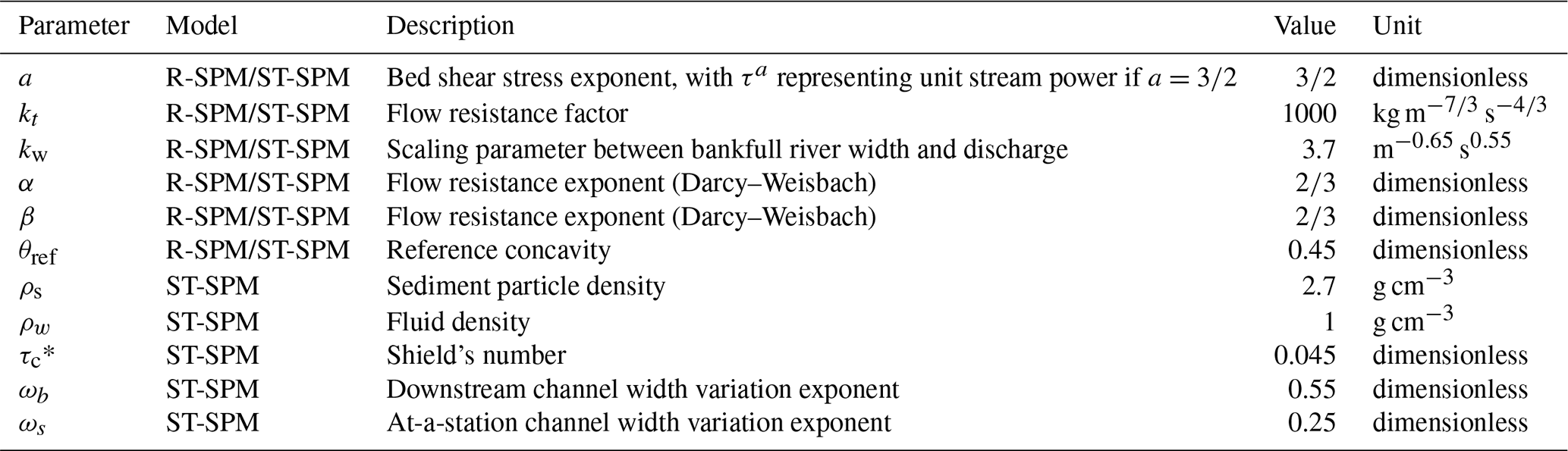
in which Q* represents the dimensionless normalized daily discharge calculated by dividing daily discharge Q (L3 T−1) by mean annual discharge (L3 T−1), ke (L2.5 T2 m−1.5) is the erosional efficiency constant, (L T−1) is the mean annual runoff, a is the shear stress exponent reflecting the nature of the incision process (Whipple et al., 2000), ψ is the threshold term (L T−1), and kt, kw, α, β, ωa and ωb are the channel hydraulic parameters described in Table 1.
In a second step, long-term river incision is calculated by multiplying instantaneous river incision, I, calculated for a discharge of a given magnitude (Q*) with the probability for that discharge to occur (pdf(Q*)), and subsequently integrating this product over the range of possible discharge events specific to the studied timescale (DiBiase and Whipple, 2011; Lague et al., 2005; Scherler et al., 2017; Tucker and Bras, 2000; Tucker and Hancock, 2010):
in which is the minimum normalized discharge required to exceed the critical shear stress (τc), and is the maximum possible normalized discharge over the time considered.
1.2.3 Runoff-Based Stream Power Model
The Runoff-Based Stream Power Model (R-SPM) is a simplified version of the Stochastic-Threshold Stream Power Model (ST-SPM). The R-SPM assumes that the incision thresholds are negligible (ψ=0) and that discharge is constant over time (, simplifying Eq. (5) to
In the following sections, we first describe the study area, characterize the lithological configuration by developing a lithological erodibility index and compile a database to represent runoff variability. Second, we present the methods and assumptions used for calibrating and simulating river incision. In a third section, the modeling results are presented at the catchment scale: we start by evaluating the impact of lithological heterogeneity on river incision rates using an area-based river incision model (A-SPM). We then evaluate to what extent the variability in denudation rates can be explained by spatial and/or temporal runoff variability and the existence of incision thresholds using the R-SPM and ST-SPM. In a final section, we discuss our findings, highlight the implications of our work and discuss further perspectives.
2.1 Tectonics and geomorphic setting
The Paute catchment is a 6530 km2 transverse drainage basin (2.9∘ S, 79∘ W): the Paute River has its source in the eastern flank of the Western Cordillera, traverses the Cuenca intramontane basin and cuts through the Eastern Cordillera before joining the Santiago River, a tributary of the Amazon (Fig. 1; Hungerbühler et al., 2002; Steinmann et al., 1999). Where the Paute River cuts through the Eastern Cordillera, the topography is rough with steep hillslopes (90th percentile of slope gradients: 0.40 m m−1) and deeply incised river valleys (Guns and Vanacker, 2013).
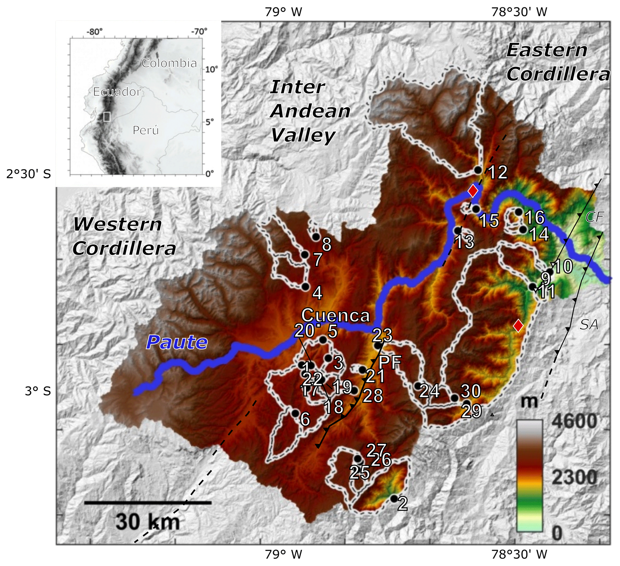
Figure 1Geomorphic setting of the Paute catchment. The numbered dots indicate the sampling locations for the CRN-derived erosion rates and their corresponding watersheds (Table 2). Solid black lines indicate the major faults. PF: the Peltetec Fault, CF: the Cosanga Fault, SA: the sub-Andean thrust fault. Concealed faults separating major stratigraphical units are indicated with dashed lines. The location of Quaternary faults is derived from the international lithosphere program (http://geology.cr.usgs.gov). Major knickpoints are indicated as red diamonds. The color scale indicates elevations, which were derived from the 30 m SRTM v3 DEM (Farr et al., 2007). The main map is produced with Topo Toolbox (Schwanghart and Scherler, 2014). The inset map is made in QGis 3 ©.
The oblique accretion of terranes to the Ecuadorian margin during the Cenozoic resulted in a diachronous exhumation and cooling history along the Ecuadorian cordillera system (Spikings et al., 2010). South of 1.5∘ S, where the Paute basin is situated, three distinct periods with a higher cooling rate have been reported during the Paleogene at 73–55, 50–30 and 25–18 Ma, corresponding to a total cooling from ca. 300 to ca. 60∘ C (Spikings et al., 2010). In the Western Cordillera, no elevated cooling is observed during the Paleogene and extensional subsidence of the Cuenca basin allowed synsedimentary deposition of marine, lacustrine and terrestrial facies until the Middle to Late Miocene (Hungerbühler et al., 2002; Steinmann et al., 1999). The collision between the Carnegie ridge and Ecuadorian trench at some time between the Middle to Late Miocene (Spikings et al., 2001) resulted in uplift of the Western Cordillera and caused a tectonic inversion of the Cuenca basin (Hungerbühler et al., 2002; Steinmann et al., 1999). Based on a compilation of mineral cooling ages available for the Cuenca basin, Steinman et al. (1999) estimated a mean rock uplift rate of ca. 0.7 mm yr−1 and a corresponding surface uplift of ca. 0.3 mm yr−1 from 9 Ma to present. Uplift patterns are assumed to be reflected in the river steepness and not explicitly simulated in this paper.
The Paute basin is characterized by a tropical mountain climate (Muñoz et al., 2018). Despite the presence of mountain peaks up to ca. 4600 m (Fig. 1), the region is free of permanent snow and ice (Celleri et al., 2007). The region's precipitation is regulated by its proximity to the Pacific Ocean (ca. 60 km distance), the seasonal shifting of the Intertropical Convergence Zone (ITCZ) and the advection of continental air masses sourced in the Amazon basin, giving rise to an orographic precipitation gradient along the eastern flank of the Eastern Cordillera (Bendix et al., 2006). Total annual precipitation is highly variable within the Paute basin and ranges from ca. 800 mm in the center of the basin up to ca. 3000 mm in the eastern parts of the catchment (Celleri et al., 2007; Mora et al., 2014).
2.2 Lithological strength
The erodibility map was developed using an empirical, hybrid classification method: it combines information on the lithological composition (Aalto et al., 2006) and the age of non-igneous formations assuming higher degrees of diagenesis and increased lithological strength for older formations (see Kober et al., 2015). Adding age information to evaluate lithological strength has advantages because lithostratigraphic units are typically composed of different lithologies but mapped as a single entity because of their stratigraphic age. The lithological erodibility (LE) is calculated as
LA is a dimensionless erodibility index based on stratigraphic age (Fig. 2a), and LL is a dimensionless erodibility index based on lithological strength (Table 3), similar to the erodibility indices published by Aalto (2006). Note that LA varies between 1 (Carboniferous) and 6 (Quaternary), whereas LL ranges between 2 (e.g., granite) and 12 (e.g., unconsolidated colluvial deposits). The lithological strength thus has a double weight, resulting in L′ values ranging between 1 and 6. For igneous rocks, only LL is considered, assuming that the lithological strength of igneous rocks remains constant over time. For river incision parameters to be comparable to other published ranges, LE is finally scaled around 1 by multiplying L′ with 2∕7. LE therefore ranges between 2∕7 and 12∕7. A description of the lithological units, the age of the formations and their lithological strength (LA, LL and LE) is provided in Supplement Table S3.
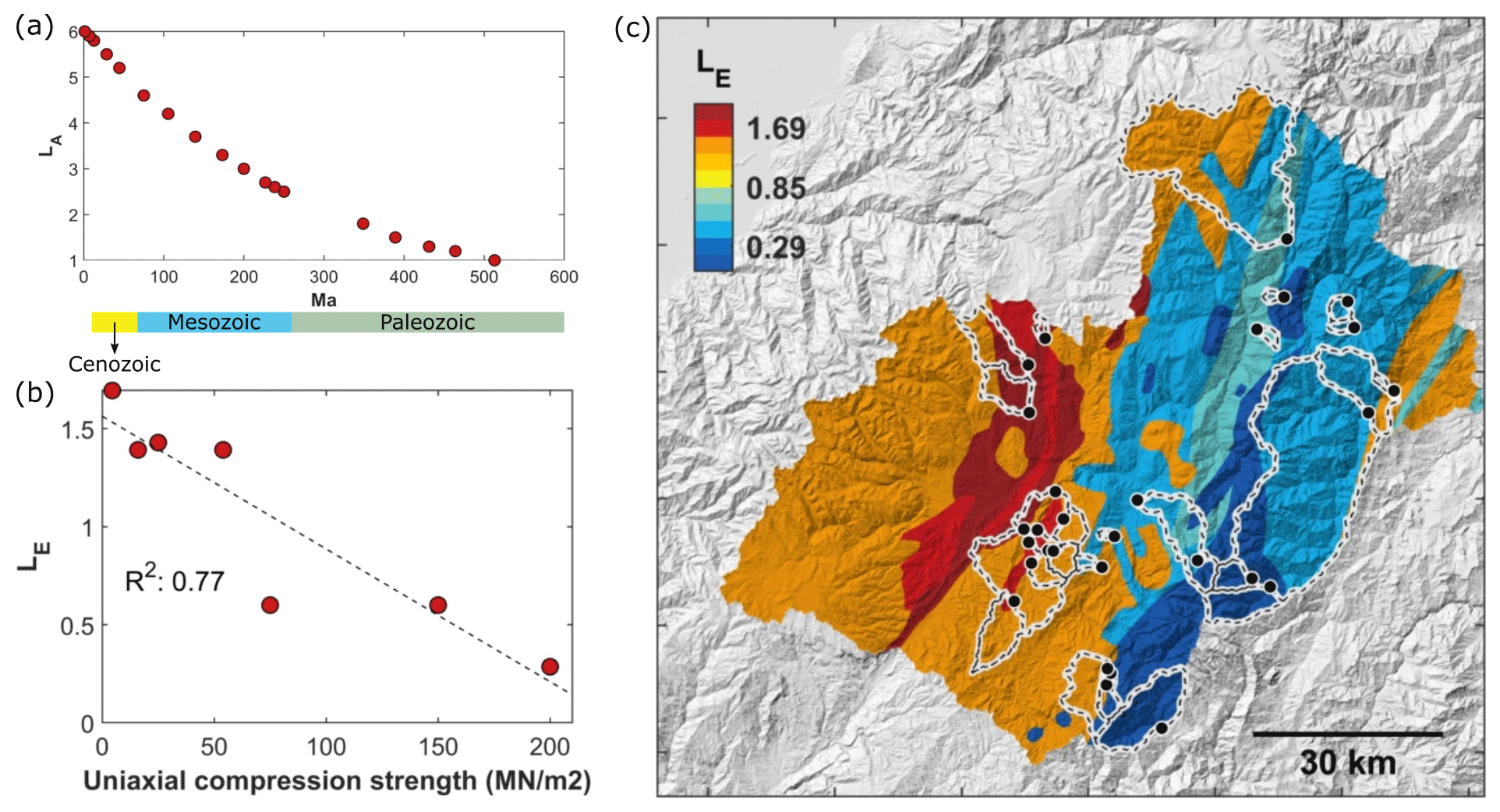
Figure 2Development of empirical lithological erodibility index (LE) and its application to the Paute catchment. (a) Proposed lithological erodibility index based on lithological age (LA). Detailed sub-classifications per lithology can be found in Table S1. (b) Field measurements of uniaxial compressive strength (Basabe, 1998; Table S4) versus the empirical erodibility index calculated using Eq. (7). Note that two of the nine observations overlap on this plot. (c) Spatial distribution of LE in the Paute catchment. The underlying topographic map is based on the 30 m SRTM v3 DEM (Farr et al., 2007). The lithological erodibility map for Ecuador was used to delineate different lithostratigraphic units and is based on the 1M geological map of Ecuador (Egüez et al., 2017; see also Fig. S1 in the Supplement). The map is produced with Topo Toolbox (Schwanghart and Scherler, 2014).
Using Eq. (7), we developed the erodibility map of Ecuador (Fig. S1) and the Paute catchment (Fig. 2c) based on the 1M geological map of Ecuador (Egüez et al., 2017). The lithological erodibility values were compared with field measurements (n=9) of bedrock rheology by Basabe (1998). An overview of measured lithological strength values is provided in Table S4 (e.g., uniaxial compressive strength). Figure 2b shows good agreement (R2=0.77) between the lithological erodibility index, LE, and the measured uniaxial compressive strength.
2.3 CRN-derived denudation rates
Catchment-wide denudation rates are derived from in situ produced 10Be concentrations in river sand. At the outlet of 30 sub-catchments (Fig. 1, Table 2), fluvial sediments were collected. We refer to Vanacker et al. (2015) for details on sample processing and derivation of CRN denudation rates taking into account altitude-dependent production, atmospheric scaling and topographical shielding (Dunai, 2000; Norton and Vanacker, 2009; Schaller et al., 2002). CRN concentrations are not corrected for snow or ice coverage because there is no evidence of glacial activity during the integration time of CRN-derived denudation rates (Vanacker et al., 2015). Three data points were excluded from model optimization runs: two catchments with a basin area smaller than 0.5 km2 (MA1 and SA) and one catchment with an exceptionally low 10Be concentration that can be attributed to recent landslide activity (NG-SD; see Vanacker et al., 2015).
Table 2Characteristics of the sub-catchments studied in this paper. IDs correspond to the numbers indicated in Fig. 1. The 10Be cosmogenic nuclide erosion rates were derived from Vanacker et al. (2015)a. Coordinates are given in decimal degrees in the WGS84 datum, is the average lithological index for the catchment, ksn is the normalized catchment average steepness, PRIDW and RRIDW are respectively the downscaled catchment average precipitation and runoff, and k is the optimized discharge variability coefficient (see Eq. 9).
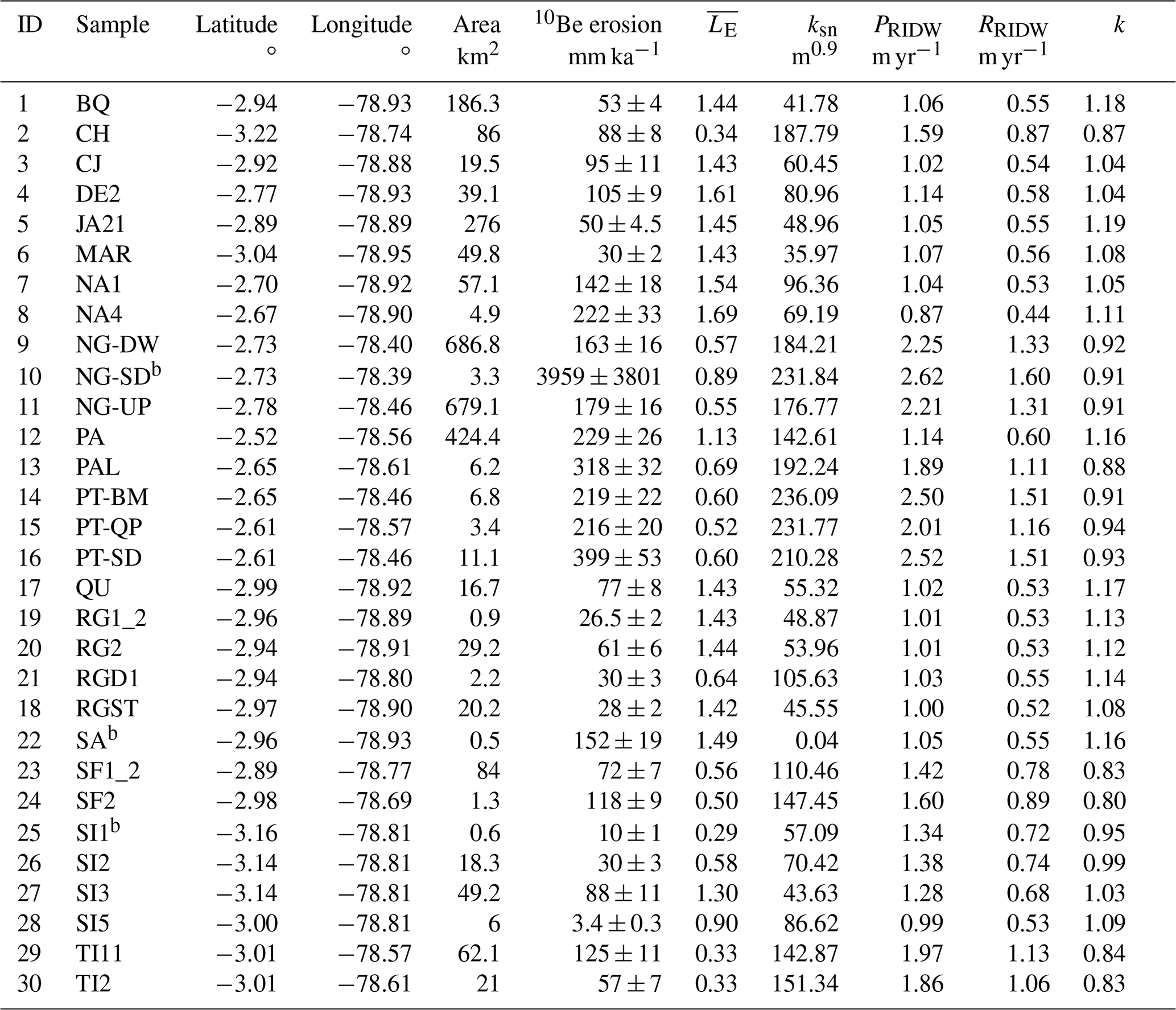
a Catchment MA1 from Vanacker et al. (2015) is not listed because its area (< 0.1 km2) did not allow us to accurately calculate the catchment properties listed here. b Catchments excluded from model optimization runs (see text).
2.4 River morphology
Based on a gap-filled SRTM v3 digital elevation model (DEM) with 1 arcsec resolution (Farr et al., 2007), we calculate river steepness for all channels with drainage areas > 0.5 km2 and average it over 500 m reaches. The optimized concavity θ for the Paute catchment (0.42; Text S1) is close to the frequently used value of 0.45, so we fix concavity to the reference value of 0.45 and report river steepness as normalized river steepness (ksn) in the remainder of this paper. The spatial pattern of ksn values (Fig. 3) is a result of the transient geomorphic response to river incision initiated at the Andes Amazon transition zone (Vanacker et al., 2015). To evaluate the extent to which transient river features influence simulated denudation rates, chi plots (χ) for all studied sub-catchments are calculated following Royden and Perron (2013) and given in the Supplement (Text S1; Fig. S4; Royden and Perron, 2013).
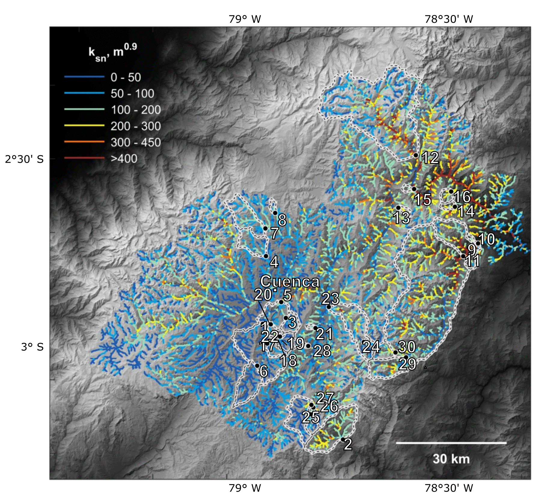
Figure 3Normalized steepness (ksn) for the Paute basin. Calculated ksn values for the Paute basin are overlain with a hillshade map (based on the 30 m SRTM v3 DEM; Farr et al., 2007). The highest values can be observed in two major knickzones located in the lower part of the Paute basin. In these zones, topographic rejuvenation started and a transient incision pulse has propagated from east to west (see also Fig. S3). The map is produced with Topo Toolbox (Schwanghart and Scherler, 2014).
To constrain the value of kw used in the process-based incision models (Eqs. 4 and 6), we calibrate the relationship between bankfull river width (Wb) and discharge (Leopold and Maddock, 1953):
in which kw () and ωb are scaling parameters regulating the interaction between mean annual discharge and incision rates (Eq. 4). We constrain kw by analyzing downstream variations in bankfull channel width for a fraction of the river network (see Scherler et al., 2017). River sections are selected based on the availability of high-resolution optical imagery in Google Earth, and river width was derived using the ChanGeom toolset (Fisher et al., 2013; Fig. S5).
The power-law fit between Q and W yields a value of 0.43 for the scaling exponent, ωb, with an R2 of 0.51 (Fig. 4). The value of this exponent lies within the range of published values of 0.23–0.63 (Fisher et al., 2012; Kirby and Ouimet, 2011). To maintain a dimensionally consistent stream power model, ωb was fixed to a value of 0.55. When doing so, the fit remains good (R2=0.5) and we obtained a kw value of 3.7 m−0.65 s0.55 that is used in the remainder of the paper.
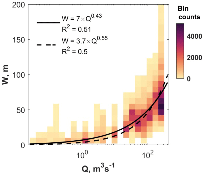
Figure 4River width (W) as a function of the mean annual discharge (Q). W represents bankfull channel width for a selected number of river sections. These were digitized in Google Earth using the ChanGeom toolset (Fisher et al., 2013; Fig. S5). Mean annual water discharges (Q) were derived from the downscaled RRIDW WRR2 WaterGAP3 data (available from http://www.earth2observe.eu; see Sect. 2.4).
2.5 Runoff variability
Evaluating the role of spatial and temporal runoff variability (Eqs. 5 and 6) requires estimates of catchment-specific runoff (, spatial variability) and discharge (temporal variability). Although measured runoff data and discharge records are available for the Paute basin (Molina et al., 2007; e.g., Mora et al., 2014; Muñoz et al., 2018), the monitoring network of existing hydrological stations does not capture the spatial variability present in the different sub catchments of the 6530 km2 Paute basin (Fig. 1). To estimate runoff variability for all 30 sub-catchments, we use hydrological data derived in the framework of the Earth2Observe Water Resource Reanalysis project (WRR2; Schellekens et al., 2017) available from 1979 to 2014. Specifically, we use the hydrological data calculated with the global water model WaterGAP3 (Water – Global Assessment and Prognosis: Alcamo et al., 2003; Döll et al., 2003) at a spatial resolution of 0.25∘ and a daily temporal resolution (http://www.earth2observe.eu, last access: 19 May 2020). Uncertainties associated with the WaterGAP3 data originate from hydrological model assumptions and spatially distributed input data (Beck et al., 2017). We revisit the impact of uncertainties in the climatological data on our model runs in the Discussion section of this paper. In the following paragraphs, we explain how we derive (i) a high-resolution runoff map by spatially downscaling these coarse data and (ii) catchment-specific magnitude frequency distributions of discharge (pdf_Q*) characterizing the temporal variability of runoff.
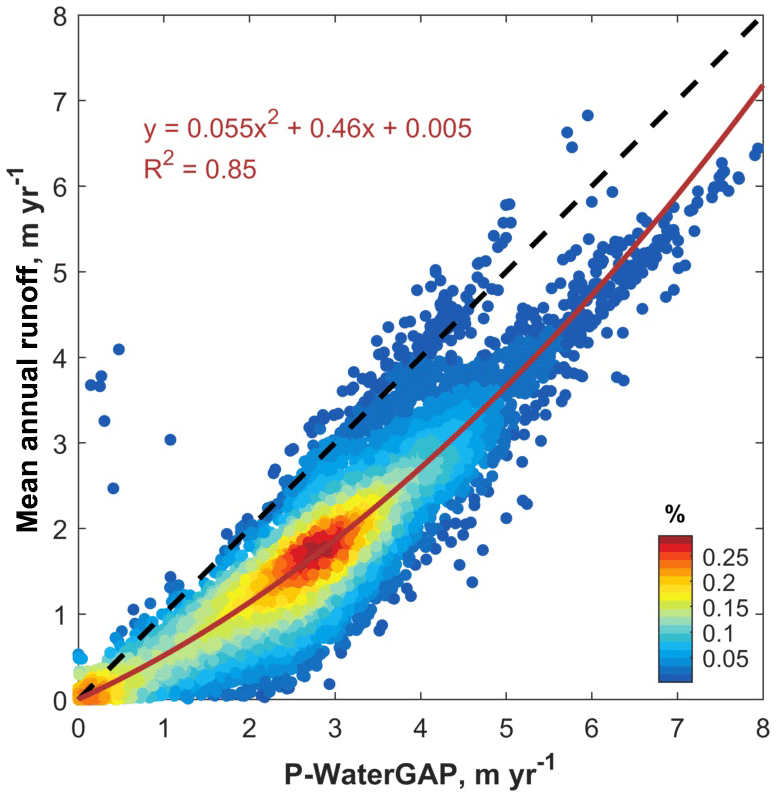
Figure 5Calibration of the precipitation (P) versus runoff curve (R). Mean annual runoff versus the mean annual precipitation for all WaterGAP3 pixels in Ecuador (0.25∘; 1979–2014; WaterGAP3 data available from http://www.earth2observe.eu).
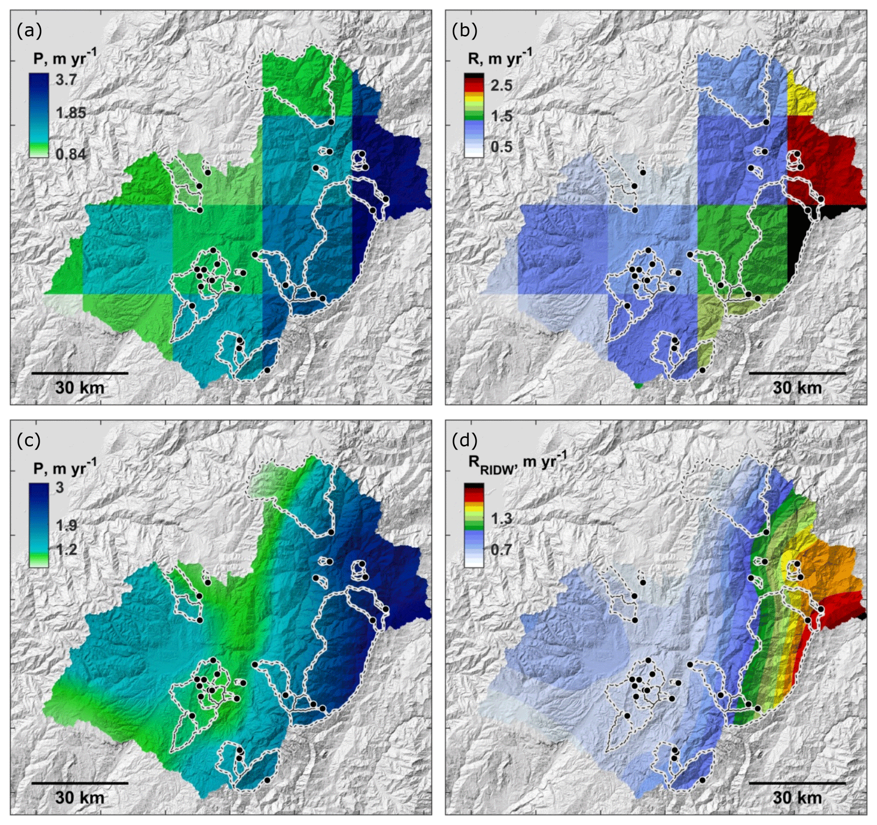
Figure 6Downscaling of WRR2 WaterGAP3 rainfall and runoff products to high-resolution regional maps. (a) WRR2 WaterGAP3 precipitation (P) at the original resolution of 0.25∘. (b) Corresponding runoff (R) at the original resolution of 0.25∘. (c) Downscaled precipitation (PRIDW) at a resolution of 2500 m, and (d) corresponding downscaled runoff (RRIDW) at a resolution of 2500 m. WaterGAP3 data were derived from earth2observe.eu. The underlying hillshade maps are based on the 30 m SRTM v3 DEM (Farr et al., 2007). The maps are produced with Topo Toolbox (Schwanghart and Scherler, 2014).
2.5.1 Spatial runoff patterns
A global hydrological reanalysis dataset such as WaterGAP provides daily runoff data over several decades and makes our methodology transferable to other regions. However, a spatial resolution of 0.25∘ is insufficient to represent highly variable regional trends in water cycle dynamics over mountainous regions (Mora et al., 2014) and in small catchments. Therefore, we downscale the Ecuadorian WaterGAP3 data to a resolution of 2.5 km by amalgamating rain gauge data with the reanalysis product. The procedure consisted of the following steps and is presented in Figs. 5 and 6.
The relationship between precipitation (P) and runoff (R) is constrained from the fit between monthly mean values for P and R available for all Ecuadorian WaterGAP 0.25∘ pixels (Fig. 5).
A high-resolution mean annual precipitation map (PRIDW) is calculated by downscaling the WaterGAP precipitation data (P) using a series of rain gauge observations (338 stations, 1990–2013) from the Ecuadorian national meteorological service (INAMHI; available from http://www.serviciometeorologico.gob.ec/biblioteca/, last access: 19 May 2020). A residual inverse distance weighting (RIDW) method is applied to amalgamate mean annual gauge data with the mean annual WaterGAP3 precipitation map. First, the differences between the gauge and WaterGAP data are interpolated using an IDW method (Fig. S6). Second, the resulting residual surface is added back to the original P data. A similar approach is often applied to integrate gauge data with satellite products, and we refer to the literature for further details on its performance (e.g., Dinku et al., 2014; Manz et al., 2016). Figure 6a shows P for the Paute region, and Fig. 6c shows its downscaled equivalent (PRIDW).
Daily precipitation data (12 784 daily grids between 1979 and 2014) are downscaled to 2.5 km using the ratio between PRIDW and P, thereby assuming that the mean annual correction for precipitation also holds for daily precipitation patterns.
The relationship between P and R (Fig. 5) is used to derive daily runoff values from the downscaled precipitation data for every day between 1979 and 2014.
The mean annual runoff map for the Paute basin is shown in Fig. 6b and its downscaled equivalent in Fig. 6d. Mean annual values are further used to calculate mean catchment runoff () and the discharge variability (next paragraph) for every sub-catchment described in Table 2. The mean catchment-specific runoff averaged for all catchments equals 0.82±0.35 m yr−1.
2.5.2 Frequency magnitude distribution of orographic discharges
Runoff variability is typically cast in terms of spatial runoff variability (Sect. 2.4.1). However, the temporal pattern of runoff might also influence river incision and is typically represented by discharge magnitude frequency distributions. Constraining the shape of these distributions is important because the number of large storm events determines the frequency with which thresholds for river incision to occur are exceeded (see Sect. 1.2.2 and references therein).
The probability distribution of discharge magnitudes consists of two components: at low discharges, the frequency of events increases exponentially with increasing discharge (Lague et al., 2005), whereas at high discharge, the frequency of events decreases with increasing discharge following a power-law distribution (Molnar et al., 2006). An inverse gamma distribution captures this hybrid behavior and can be written as (Crave and Davy, 2001; Lague et al., 2005)
in which Γ is the gamma function and k is a discharge variability coefficient; k represents the scale factor of the inverse gamma distribution and (k+1) the shape factor. Previous studies used a single average k value to characterize regional discharge: DiBiase and Whipple (2011) use a constant k value for the San Gabriel Mountains, whereas Scherler et al. (2017) use a constant k value for high and low discharge but distinguish between eastern Tibet and the Himalaya. However, given the strong variation in temporal precipitation regimes in the Paute basin (Celleri et al., 2007; Mora et al., 2014), we explicitly evaluated the role of temporal runoff variability by calculating catchment-specific discharge distributions from the WRR2 WaterGAP dataset.
Daily variations in discharge at the sub-catchment outlets (Fig. 1) were calculated by weighing flow accumulation with runoff (RRIDW; see Sect. 5.1.1). For every catchment, the complementary cumulative distribution function (CCDF) of the daily discharge was fitted through the observed discharge distribution as
where Γ is the lower incomplete gamma function. Figure S7 illustrates the fit between the WaterGAP-derived discharge distribution and the optimized CCDF for one of the catchments. Site-specific discharge variability values (k) are calculated for all catchments and listed in Table 2. The obtained k values range between 0.8 and 1.2 with a mean of 1.01±0.12.
The presented river incision models (A-SPM, R-SPM and ST-SPM in Sect. 1.2) all depend on river steepness, ksn, which is known to correlate well with ECRN (DiBiase et al., 2010; Ouimet et al., 2009; Scherler et al., 2017; Vanacker et al., 2015). Moreover, ECRN integrates over time spans that average out temporal fluctuations of denudation rates and over spatial extents that are sufficient to average out the erratic nature of hillslope processes. Therefore, ECRN can be used to constrain models of river incision provided a set of assumptions that we first describe below.
3.1 CRN-derived denudation rates to calibrate river incision
The use of CRN-derived denudation rates to calibrate river incision relies on three main assumptions, summarized by Scherler et al. (2017). A first assumption is that the catchment-wide denudation rates derived from CRN are representative for long-term fluvial incision. Positive correlations between river steepness, ksn, and CRN-derived denudation rates support this assumption (Vanacker et al., 2015), except for very small catchments where CRN-derived denudation rates are sensitive to the occurrence of deep-seated landslides during which material shielded at depth is supplied to the river (Niemi et al., 2005; Yanites et al., 2009). A second assumption when using CRN data to calibrate river incision models is that the sediment cosmogenic nuclide budget is at steady state at the catchment scale so that the input of CRN via in situ production equals the export of CRN via sediment export and radioactive decay. Given the size of the studied basins, this assumption seems to be reasonable. A third assumption, in particular when using the process-based R-SPM and ST-SPM, is that the runoff data used to calibrate the incision parameters are uniform within the sampled sub-catchments and representative of the time span over which CRN data integrate (1–100 kyr). This is a challenging assumption given that available hydrological data only cover the recent past. While spatial patterns of runoff, mainly controlled by orographic precipitation, could be assumed to be broadly similar over the integration time of CRN-derived denudation, this is not necessarily true for the temporal variation in runoff. We will revisit the validity and implications of these three assumptions in the Discussion section of this paper.
3.2 River incision models
In a first set of model runs, we evaluate the performance of the area-based SPM (A-SPM) in predicting ECRN rates. To account for rock strength variability Eq. (2) is rewritten as
where ka (L1−2m T−1) is the erosional efficiency parameter and is a dimensionless catchment mean lithological erodibility value. Given its empirical nature, wherein the effect of allogenic (e.g., runoff variability) and autogenic (e.g., incision thresholds and river width dynamics) controls of fluvial processes is integrated within the empirical scaling parameters (K, m and n), the A-SPM does not enable us to identify the role of spatial or temporal runoff variability and incision thresholds. Note that, at any point in the paper, lithological heterogeneity within the Paute catchment is represented using the average values of LE for the individual sub-catchments indicated with and listed in Table 2. If lithological heterogeneity is not considered, is fixed to a value of 1.
In a second set of model runs, we evaluate to what extent more advanced SPMs can be used to understand the role of these allogenic and autogenic processes. We start by evaluating the performance of a runoff-based SPM (R-SPM). To account for rock strength variability Eq. (6) is rewritten as
An overview of the parameter values required to solve the R-SPM is given in Table 1. Only the value of kw is based on a regional calibration of the hydraulic geometry scaling (see Sect. 2.3). Other parameters are set to theoretical values (reported by Deal et al., 2018; DiBiase and Whipple, 2011; Scherler et al., 2017). Actively incising bedrock channels are often covered by a layer of sediment (Shobe et al., 2017). Therefore, we assume that river incision is scaled to the bed shear stress as for bedload transport (Meyer-Peter and Müller, 1948) and set a to 3∕2 (see DiBiase and Whipple, 2011; Scherler et al., 2017). We use the Darcy–Weisbach resistance relation and coefficients () to calculate shear stress exerted by the river flow on its bed and assume a friction factor of 0.08, resulting in a flow resistance factor kt of 1000 kg m s (e.g., Tucker, 2004). The use of Darcy–Weisbach friction coefficients in combination with results in a value for the slope exponent equal to unity (n=1; see Eq. 4). Based on these theoretical derivations, we fix n to unity when constraining the R-SPM. Note that this contrasts with the first set of model runs (application of the A-SPM) in which we allow n to vary. By fixing n to unity, we want to verify whether spatial variations in runoff (incorporated in K from Eq. 12) can explain variations in incision rates otherwise ascribed to nonlinear river incision. The only parameter not fixed to a constant value is the erosivity coefficient ke, which is optimized as described in Sect. 3.3.
In a final set of model runs, we apply the Stochastic-Threshold SPM (ST-SPM) to evaluate the role of temporal precipitation variability and thresholds for incision (Eq. 4). Here, we adjust the ST-SPM to account for rock strength variability as
To derive long-term erosion rates (E), Eq. (13) is integrated over the probability density function of discharge magnitudes (Eq. 5), which requires values for the lower () and the upper () limit of the integration interval. Constraining is difficult based on observational records alone as they might miss some of the most extreme flooding events. However, when simulating incision rates over long time spans and thus considering long return times of (> 1000 years), the solution of Eq. (5) is insensitive to the choice of (Lague et al., 2005). We therefore set to infinity in all our model runs. The critical discharge () for erosion to occur can be derived from Eq. (13) by setting I equal to 0:
The impact of spatial variations in runoff and discharge variability is evaluated by setting and k to the sub-catchment-specific values or the mean of these values (listed in Table 2; Eq. 4). The parameters left free during optimization are the erosivity coefficient ke and the critical shear stress . Parameter values of both variables are optimized as described in Sect. 3.3.
3.3 Optimization of model parameters
We propose three metrics to evaluate the performance of the river incision models. The first one is the commonly used model error (ME),
where nb is the number of ECRN data points, Oi represents the catchment-specific measured ECRN denudation rates, Mi represents the catchment-specific modeled river incision and σi represents the catchment-specific standard deviation of ECRN. The advantage of the ME is that it explicitly incorporates the error on the analytical data (ECRN) by weighing the model error with the analytical error. However, errors on CRN data are heteroscedastic: they systematically increase with increasing denudation rates. Although the ME thus provides a good metric to evaluate overall model performance, the metric is not well suited to optimize model parameters in an optimization procedure: too much weight will be given on optimization of the model in the lower regime of the denudation spectrum in which measured errors on ECRN are low, whereas higher measured ECRN data will not be approximated well because of large associated errors. To compensate for the effect of heteroscedasticity we rescale values Oi, Mi and Ei using a logarithm with base 10 when calculating ME (Herman et al., 2015). In this paper, ME will be used to evaluate model performance but not to optimize model parameters.
A second metric is the coefficient of determination, R2:
where fi represents the fitted ECRN denudation rates. Contrary to ME, R2 evaluates the explained variance of the model by giving all observations the same weight, regardless their analytical error. However, when model parameters result in an offset between simulated and observed data (i.e., the intercept of the fit), this can still result in a high R2.
We therefore use the Nash–Sutcliffe model efficiency to optimize model parameters (NS; Nash and Sutcliffe, 1970):
The NS coefficient ranges between −∞ and 1, where 1 indicates optimal model performance explaining 100 % of the data variance. When NS =0, the model is as good a predictor of the mean of the observed data. When NS < =0, the model performance is unacceptably low. The NS coefficient was developed in the framework of hydrological modeling but has been applied in a wide range of geomorphologic studies (e.g., Jelinski et al., 2019; Nearing et al., 2011).
In the following sections, we compare simulated erosion rates, obtained with the river incision models presented in Eqs. (11)–(13), with measured CRN-derived denudation rates. We start with the use of the A-SPM (Eq. 11) to evaluate the extent to which lithological variability controls denudation rates. Once the impact of lithological heterogeneity on river incision is clarified, we evaluate whether runoff variability and incision thresholds can explain variations in ECRN-derived denudation rates. To this end, two river incision models are evaluated (the R-SPM and ST-SPM, presented in Eqs. 12 and 13, respectively). The optimized parameters and model performance of all model scenarios are listed in Table 4. Best-fit results of a selected number of model runs are presented in Figs. 7 and 8. An overview of model fits for all the scenarios listed in Table 4 is given in Figs. S8, S9 and S10.
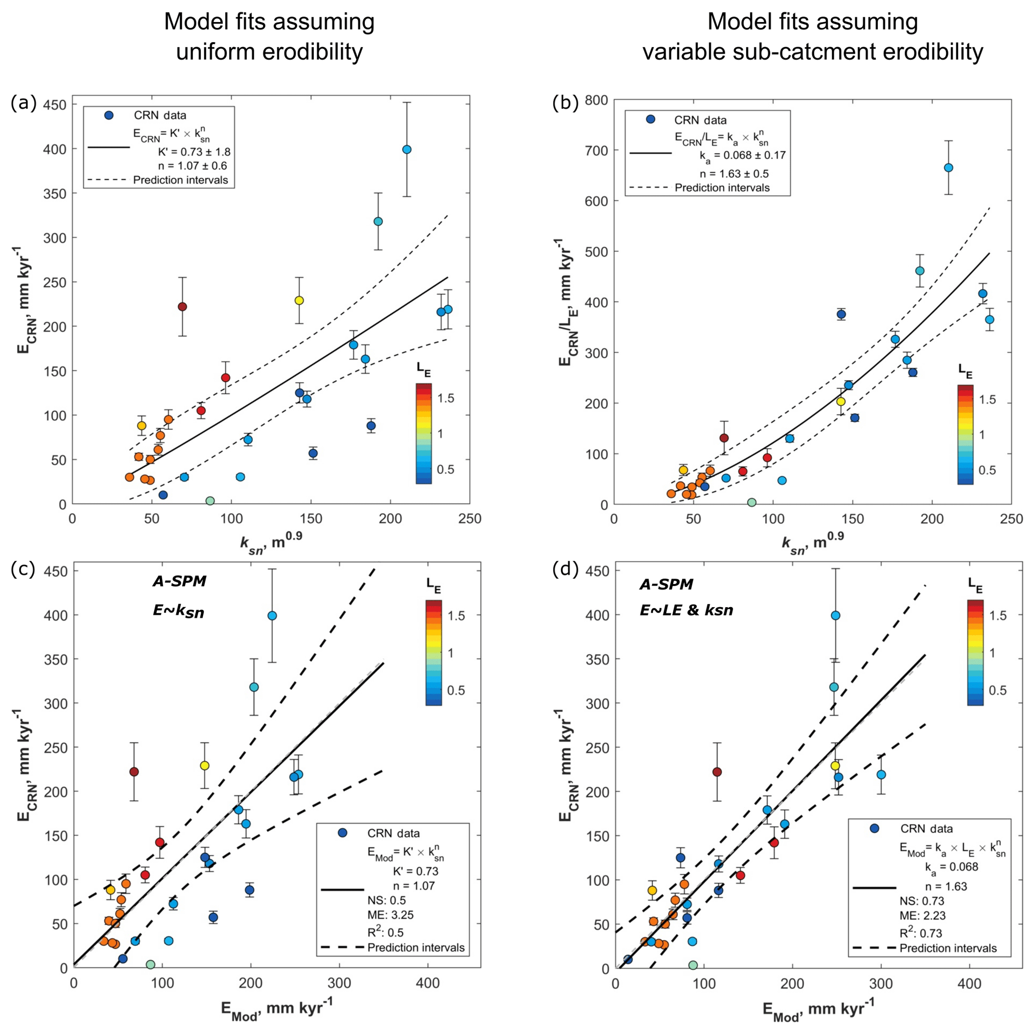
Figure 7Best fit between CRN-derived erosion rates (ECRN) and river steepness index (ksn) or modeled river incision (EMod) using the Area-Based Stream Power Model (A-SPM). (a) Measured ECRN versus ksn (Table 2). Observations are colored according to the average lithological erodibility of the sub-catchment (). Low values for represent strong rocks that are resistant to erosion. High values for represent weak rocks that are susceptible to erosion. (b) Measured ECRN divided by versus ksn (Table 2). By correcting the ECRN values for lithological heterogeneity, the ksn−ECRN relationship becomes significantly nonlinear (). (c) A-SPM scenario 1 (see Table 4). Modeled erosion rates for catchments consisting of strong rocks (blue) are mostly overpredicted and plot below the 1:1 line. Modeled erosion rates for catchments consisting of weak rocks (red) are mostly underpredicted and plot above the 1:1 line. (d) A-SPM scenario 2 (Table 4) in which spatially variable lithological erodibility is explicitly accounted for. A complete overview of all best model fits for A-SPM scenarios 1–4 is given in Fig. S8.
Table 3Lithological erodibility index values based on the lithological strength (LL; Eq. 7). Detailed sub-classifications per lithology can be found in Table S2.
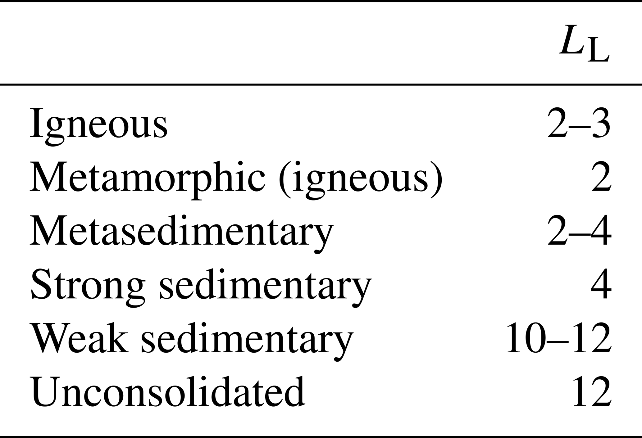
Table 4Overview of the best-fit model results.
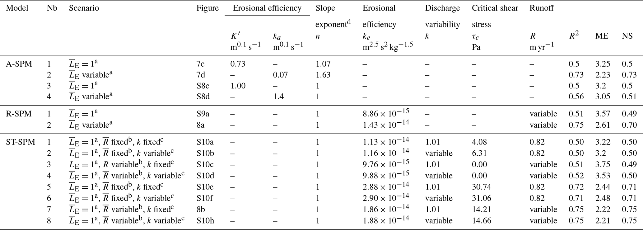
a If is variable, catchment-specific values for LE are used (Table 2). b If R is fixed, a uniform mean runoff value of 0.8 m yr−1 is used for all catchments. If R is variable, catchment-specific values are used (Table 2). c If k is fixed, a uniform mean discharge variability value of 1.01 is used for all catchments. If k is variable, catchment-specific values are used (Table 2). d The slope exponent (n) is optimized as a free parameter in A-SPM 1–2. It is fixed to 1 in A-SPM 3–4 (see text).
4.1 Area-based stream power model
In a first set of model runs we evaluate the use of an area-based stream power model (A-SPM) to explain observed variations in CRN-derived denudation rates (ECRN). We optimize river incision parameters for four scenarios (Table 4: A-SPM scenarios 1–4): in the first two scenarios, the slope exponent, n, is left as a free parameter. In the second two scenarios, the slope parameter is fixed to unity (n=1). Figure 7 illustrates both the ksn−ECRN (Fig. 7a and b) and corresponding EMod−ECRN relationships, wherein EMod represents the simulated river incision (Fig. 7c and d).
In A-SPM scenario 1 (Table 4, Fig. 7c), we assume a spatially uniform erodibility ( fixed to 1 in Eq. 11) and leave the erosion efficiency coefficient (K′) and the slope parameter n as free parameters during model optimization. The optimized fit between simulated erosion (E; Eq. 2) and ECRN is shown in Fig. 7c. The optimized fit results in a high degree of data scattering, resulting in an NS model efficiency of 0.5, an R2 of 0.5, an ME of 3.25, and optimized values for K′ and n of respectively 0.73 m0.1 s−1 and 1.07. The fit between ksn and ECRN (Fig. 7a) or simulated river incision and measured denudation rates (Fig. 7c) hints at the existence of a correlation between ECRN and river incision rates. The fit shown in Fig. 7c illustrates that modeled erosion rates for catchments with a low mean erodibility index (high resistance to erosion) are mostly overpredicted (plotting below the 1:1 line), whereas modeled erosion rates of catchments with a high erodibility index are mostly underpredicted (plotting above the 1:1 line).
In A-SPM scenario 2 (Table 4, Fig. 7d), we quantify the impact of varying lithology by using sub-catchment-specific values for the lithological erodibility ( in Eq. 11) and leaving ka and n as free optimization parameters. The optimized fit between simulated river incision (E, Eq. 11) and ECRN is shown in Fig. 7d. Optimization results in an NS model efficiency of 0.73, an R2 of 0.73, an ME of 2.23, and optimized values for ka and n of respectively 0.07 m0.1 s−1 and 1.63. Considering lithological erodibility strongly reduces data scatter surrounding the fit. The importance of lithological strength in controlling the A-SPM and the ksn−ECRN relation (Fig. 7b) confirms that strong metamorphic and plutonic rocks erode at slower rates than lithologies that are less resistant to weathering such as volcaniclastic deposits. The erodibility index appears to provide an appropriate scaling of relative rock strength: analysis of residuals did not reveal any significant relation of residuals with lithology. When using spatially variable, sub-catchment-specific lithological erodibility values () (Fig. 7d), the n coefficient of the SPM is considerably larger than unity (n=1.63) and the ksn−ECRN relationship becomes nonlinear (Fig. 7b), corroborating earlier empirical findings (DiBiase et al., 2010; Harel et al., 2016; Lague, 2014; Whittaker and Boulton, 2012). To evaluate the impact of a variable n exponent on the performance of the empirical A-SPM, we executed two more model optimizations.
In A-SPM scenario 3 (Table 4, Fig. S8c), we assume a spatially uniform lithology and erodibility ( fixed to 1 in Eq. 11), fix n to 1 and only leave K′ to be optimized as a free model parameter. With an NS model efficiency of 0.5, an R2 of 0.5, an ME of 3.2 and an optimized value for K′ of 1.00 m0.1 s−1, the model fit and performance are similar to the values obtained in scenario 1.
In A-SPM scenario 4 (shown in Table 4, Fig. S8d), lithological variability is considered (using sub-catchment-specific values for in Eq. 11), n is fixed to 1 and K′ is a free model parameter. With an NS model efficiency of 0.51, an R2 of 0.56, an ME of 3.05 and an optimized value for K′ of 1.4 m0.1 s−1, the model performance is much lower than when leaving the slope exponent n as a free parameter (A-SPM scenario 2).
The results from the four scenarios show that a nonlinear relationship between river steepness (ksn, representing river incision rates) and ECRN is unveiled when the lithological heterogeneity is explicitly taken into account (Fig. 7b). Likewise, a nonlinear river incision model (A-SPM scenario 2; Fig. 7d) in which lithological heterogeneity is considered outperforms the other evaluated A-SPM scenarios (Table 4).
4.2 Runoff-based and stochastic-threshold stream power models
The previous analysis shows that the explanatory power of the A-SPM model, and therefore the ksn−ECRN relationship, improves when considering spatial variations in lithology. Moreover, when considering variations in lithological erodibility, river incision is found to be nonlinearly dependent on the channel slope (S), with n=1.63. In a next step we evaluate whether this nonlinear relation can be explained by spatial and/or temporal rainfall variability and/or the existence of thresholds for river incision (Table 4: R-SPM scenarios 1–2 and ST-SPM scenarios 1–8; Fig. 8).
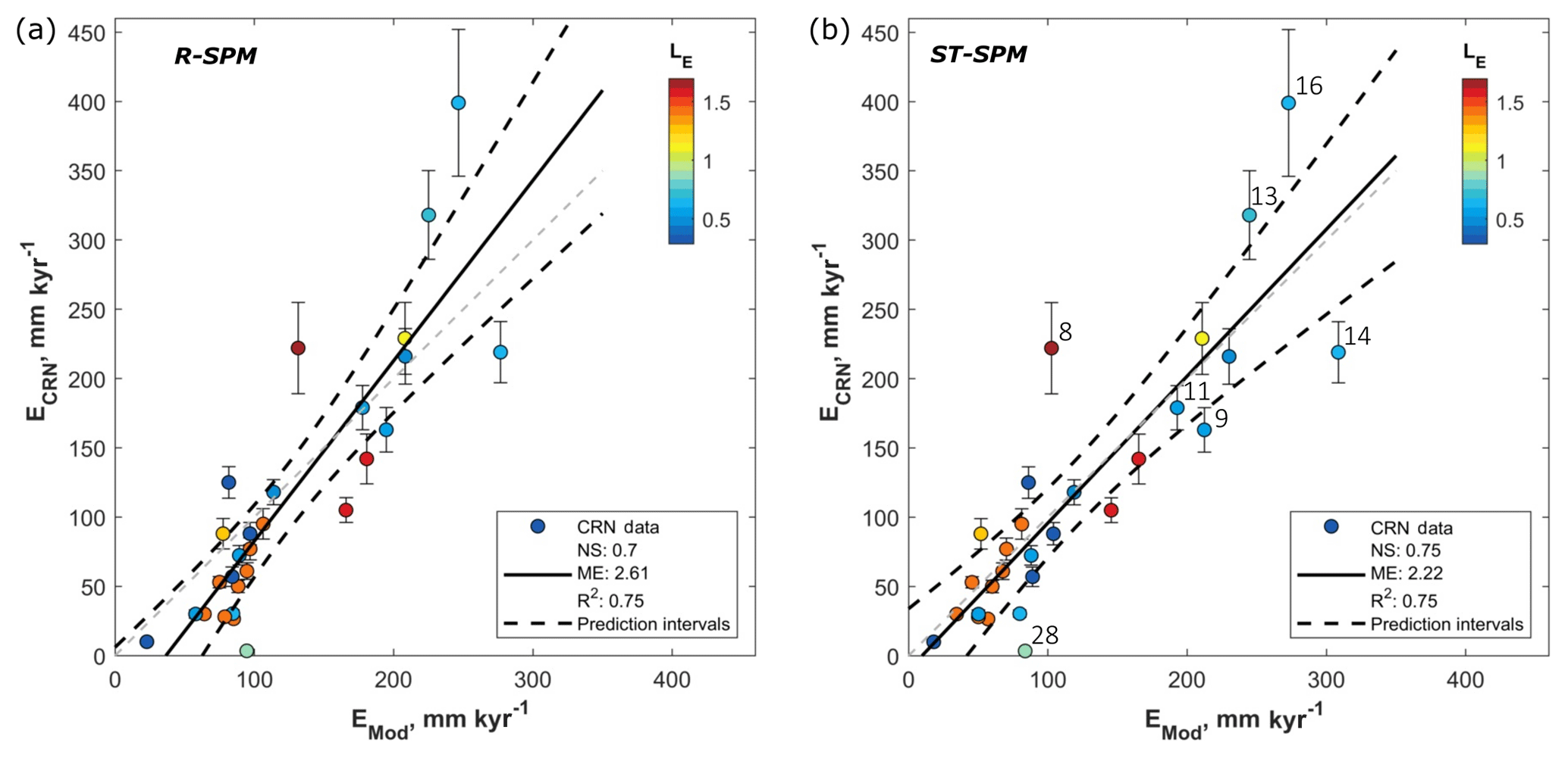
Figure 8Best fit between CRN-derived erosion rates (ECRN) and modeled river incision (EMod) using the Runoff-Based and Stochastic-Threshold Stream Power Model. (a) R-SPM scenario 2 (Table 4) using the average lithological erodibility () and runoff values per sub-catchment (both listed in Table 2). (b) ST-SPM scenario 7 (Table 4) using the average lithological erodibility () and runoff () values, as well as an incision threshold (τc=14 Pa). Numbered observations in (b) correspond to catchment IDs as listed in Table 2 (see also the discussion in Sect. 5). A complete overview of all best model fits for R-SPM scenarios 1–2 and ST-SPM scenarios 1–8 is given in Figs. S9 and S10, respectively.
4.2.1 Runoff-Based SPM (R-SPM)
In a first set of model runs, we evaluate the performance of the Runoff-Based Stream Power Model (R-SPM Eq. 12) to evaluate the role of spatially variable runoff using catchment-specific values for mean runoff (R derived from the WaterGAP data; reported in Table 2 and shown in Fig. 6).
In R-SPM scenario 1 (Table 4, Fig. S9a), lithological variability is not considered ( fixed to 1 in Eq. 12). With an NS model efficiency of 0.49, an ME of 3.57 and an R2 of 0.51, model performance is comparable to the regular A-SPM under uniform lithology with n fixed to 1 (NS = 0.5). This illustrates that studying spatial runoff variability is not feasible when ignoring the confounding role of lithological erodibility in controlling denudation rates.
In R-SPM scenario 2 (Table 4, Fig. 8a), lithological variability is considered (using sub-catchment-specific values for in Eq. 12). With an NS model efficiency of 0.7, an ME of 2.61 and an R2 of 0.75, model performance is close to that of the regular A-SPM under uniform lithology with n≫1 (NS =0.72). This model simulation therefore suggests that spatial variations in runoff can account for the nonlinearity in the ksn−ECRN relationship: while slope dependency in the R-SPM is fixed to unity (see derivation in Eq. 4a–c), the model is capable of explaining the spatial pattern in denudation rates. This implies that orographic rainfall and thus runoff gradient as shown in Fig. 6 influence the efficiency of river incision. The offset between the R2 (0.75) and NS (0.70) values can be attributed to the way in which these metrics work: whereas R2 evaluates the goodness of the linear fit between modeled and measured observations, NS evaluates the absolute differences between modeled and observed denudation rates. Hence, for the NS model efficiency to be high, observations must fit on the 1:1 line (Fig. 8a). However, most of the simulated values for low denudation rates are overestimated when using the optimized parameter values of the R-SPM and plot below the 1:1 line (Fig. 8a). Therefore, we conclude that the R-SPM performs well in predicting measured denudation rates but low denudation rates are overestimated, resulting in an NS and ME value respectively slightly lower and higher than those of the empirical A-SPM. In the following section we evaluate whether introducing temporally variable runoff coefficients and/or incision thresholds can further improve the performance of a river incision model.
4.2.2 Stochastic-Threshold SPM (ST-SPM)
In a final series of model runs, we use the Stochastic-Threshold Stream Power Model (ST-SPM, Eq. 13) to evaluate the role of spatially variable runoff (catchment-specific R; reported in Table 2 and shown in Fig. 6) in combination with catchment-specific runoff variability (k; reported in Table 2) and the presence of incision thresholds (τc in ψ in Eqs. 4 and 10). Table 4 reports details on the different model scenarios in which ST-SPM is optimized to the observed ECRN data considering all possible combinations (4) of uniform or spatially variable catchment mean runoff (R) and uniform or spatially variable catchment mean runoff variability (k). For reference, the four scenarios include both uniform and spatially variable lithological erodibility, LE (eight scenarios in total).
In ST-SPM scenarios 1–4 (Table 4, Fig. S10a–d), the ST-SPM is optimized assuming a constant erodibility (LE fixed to 1). Similar to what has been found for the R-SPM, model performance is not any better compared to the use of a simple A-SPM when not considering lithological variability. This confirms that optimizing more complex river incision models (such as the ST-SPM) has little added value when the heterogeneity in environmental conditions (lithological heterogeneity) is not considered.
In ST-SPM scenarios 5 and 6 (Table 4, Fig. S10e–f), catchment mean runoff ( is fixed to the average value of all catchments (0.82 m yr−1) in order to evaluate the role of (i) variations in observed temporal runoff variability (k) and (ii) optimized values for the incision threshold (τc). In scenario 5, k is fixed to the average value for all catchments (k=1.01), whereas in scenario 6, k is set to the catchment-specific values as listed in Table 2. Both scenarios (5 and 6) perform well with an NS value equalling 0.71, indicating that temporal runoff variability (k) is not influencing model performance. Regardless of the lack of spatially variable runoff (R), both scenarios perform as well as R-SPM scenario 2, in which runoff variability was considered. The good performance of ST-SPM scenarios 5 and 6 can be attributed to the presence of an incision threshold (ψ > 0 in Eq. 13) at which τc is optimized to a value of ca. 30 Pa (Table 4). The fact that the use of the ST-SPM with constant runoff values yields a good model fit suggests that part of the nonlinear relationship between river steepness, ksn, and ECRN can be attributed to the presence of thresholds for river incision to occur (Lague, 2014).
ST-SPM scenarios 7 and 8 (Table 4, Figs. S10e–f and 8b) are similar to scenarios 5 and 6, with the difference that spatial runoff variability is considered by using catchment-specific values for runoff (; Table 2). Similarly to scenarios 5 and 6, using catchment-specific values for k does not improve model performance, resulting in a similar model performance for scenarios 7 and 8. Overall, ST-SPM scenarios 6 and 7 result in the highest model performance of all tested scenarios, with an NS model efficiency of 0.75, an ME of 2.22 and 2.21, and an R2 of 0.75. The optimized model fit for ST-SPM scenario 7 is shown in Fig. 8b and corresponds well with the 1:1 line between modeled and observed denudation rates. Optimized values for τc are ca. 14–15 Pa, which is in the range but at the lower spectrum of earlier documented values for critical shear stress (e.g., Shobe et al., 2018, report τc values between 10 and 1000 Pa). Contrary to the R-SPM with which low denudation rates are overestimated (Fig. 8a), the ST-SPM does predict low denudation rates better due to the consideration of an incision threshold that mainly influences simulated river denudation rates at the lower end of the spectrum.
ST-SPM scenarios 7 and 8 have a model error (ME of 2.22 and 2.21, respectively) similar to the model error of A-SPM scenario 2 (ME =2.23). Hence, we conclude that an ST-SPM considering spatial variations in runoff and simulating a critical threshold for river incision performs as well as an A-SPM with the effect of allogenic (runoff variability) and autogenic (incision thresholds) response cast in the lumped empirical incision parameters. While the R-SPM and ST-SPM do not necessarily predict spatial patterns in observed ECRN rates better than an A-SPM, they do enable one to simulate the effect of runoff variability and incision thresholds, therefore providing an operational tool to simulate past and future climate changes. Note that differences in model performance between R-SPM scenario 2 and ST-SPM scenarios 5–8 are existent but not very pronounced. To evaluate the significance of these differences, our analysis should be repeated on larger datasets capturing a wider variability in denudation rates and hydrology.
5.1 Equilibrium between river incision and hillslope denudation
In theory, rates of hillslope denudation equal rates of river incision if landscapes are either in a steady state or if transient landscapes are characterized by rapid hillslope response (e.g., threshold hillslopes). Steady-state landscapes can only be achieved under stable climatic and tectonic settings that prevail over millions of years. Such stability is rarely met in tectonically active regions where landscapes continuously respond to environmental perturbations (Armitage et al., 2018; Bishop et al., 2005; Campforts and Govers, 2015).
The downstream reaches of the Paute catchment are a good example of a transient landscape where a major knickzone is propagating upstream, resulting in steep threshold topography downstream of the knickzone (Fig. S3 and Vanacker et al., 2015). Facing a sudden lowering of their base level after river rejuvenation, soil production and linear hillslope processes (Campforts et al., 2016) are no longer in equilibrium with rapidly incising rivers (Fig. 15 in Hurst et al., 2012). In steep topography, hillslopes may transiently evolve to their mechanically limited threshold slope whereby any further perturbation will result in increased sediment delivery through mass-wasting processes such as rockfall or landsliding (Bennett et al., 2016; Blöthe et al., 2015; Burbank et al., 1996; Larsen et al., 2010; Schwanghart et al., 2018). Given the erratic nature of landslides, not all threshold hillslopes will respond simultaneously to base-level lowering depending on local variations in rock strength, hydrology, land use and seismic activity (Broeckx et al., 2020; Guns and Vanacker, 2014). Therefore, catchments in transient landscapes might experience hillslope denudation with highly variable rates (Vanacker et al., 2020).
We argue that CRN-derived denudation rates in the Paute basin both overestimate and underestimate long-term incision rates in these catchments. Overestimation may result from the occurrence of recent, deep-seated landslide events, that deliver sediments with a low CRN concentration to rivers (Tofelde et al., 2018). Underestimation, in turn, may occur if long-term hillslope lowering is accomplished by rare and large landslides whose return periods exceed the integration time of CRN-derived denudation rates (Niemi et al., 2005; Yanites et al., 2009).
Longitudinal profiles of rivers draining to the knickzone in the Paute catchment show marked knickpoints. This is particularly evident in catchments 9–16 (Fig. 1) where ksn values are high (Fig. 2) and knickpoints appear in the longitudinal profiles (Figs. S3 and S4). Simulated erosion rates for some of these catchments deviate from CRN-derived denudation rates (Fig. 8b; IDs 13, 14 and 16), whereas for others (e.g., IDs 9 and 11), predictions from the stochastic-threshold river incision model show good agreement with ECRN data. For catchments with a sufficiently large drainage area, modeled incision rates correspond well with ECRN (IDs 9 and 11 being both ca. 700 km2), most likely because the mechanisms that potentially cause overestimation and underestimation cancel each other out at this scale. For smaller catchments (IDs 8, 13, 14 and 16 all being < 12 km2) there is a discrepancy between simulated river incision rates and ECRN.
Although river incision models can be used to simulate denudation patterns in large transient catchments (> 10 km2), there is a need to develop alternative approaches including landslide mechanisms in long-term landscape evolution models such as the TTLEM (Topo Toolbox Landscape Evolution Model; Campforts et al., 2017) or Landlab (Hobley et al., 2017).
5.2 Integration timescales of ECRN and ksn
Our analysis reveals the potential role of temporal and spatial variations of rainfall in long-term landscape evolution. Integration times of CRN-derived denudation rates measured in the Paute basin are of the order of 1.5–175 kyr. In contrast, response times of longitudinal river profiles generally range 0.25–2.5 Myr (Campforts et al., 2017; Goren et al., 2014; Snyder et al., 2003; Whipple, 2001; Wobus et al., 2006). During thousand-year to million-year timescales, it is unlikely that temporal rainfall distributions remain stationary. Thus, there is little reason to assume that the hydrometeorological data that we inferred from 35 years of data fully capture rainfall variability over the response times of river profiles and hillslopes. Contrary to temporal variations, the spatial patterns in orographic precipitation are characteristic of the formation of a mountain range at geological timescales (Garcia-Castellanos and Jiménez-Munt, 2015). In the southern Ecuadorian Andes, moist air advection via the South American low-level flow generates pronounced patterns of orographic precipitation (Campetella and Vera, 2002). These patterns might have persisted since at least the most recent phase of Andean uplift in the Late Miocene (Spikings et al., 2010; Spikings and Crowhurst, 2004). Present-day rainfall and runoff spatial gradients (Fig. 6) are thus deemed to be informative for spatial patterns of discharge at longer timescales (Sect. 3.1). The performance of the stream power models underscores this interpretation. While accounting for spatial patterns in runoff improves the performance of a stochastic-threshold SPM (Table 4 and Sect. 4.2.2), incorporating proxies for temporal discharge variability leads to no improvement of model performance (the role of k in Sect. 4.2.2).
5.3 Impact of lithological heterogeneity on long-term river incision rates
In all our simulations, model efficiency improves when incorporating rock strength variability (Table 4), which is consistent with earlier studies (Lavé and Avouac, 2001; Stock and Montgomery, 1999). In the absence of generally accepted metrics of erodibility, we employ an empirically derived lithological erodibility index (LE; Eq. 7) based on the age and lithological composition of stratigraphic units. Owing to its simplicity, this or a similar index can potentially be applied at continental to global scales at which information on rock physical properties is usually lacking the detail available at smaller spatial scales (Attal and Lavé, 2009; Nibourel et al., 2015). Notwithstanding, river incision also depends on other rock properties such as the density of bedrock fractures, joints and other discontinuities (Whipple et al., 2000). Fracture density has in turn been linked to spatial patterns of seismic activity (Molnar et al., 2007). Given the limited variability of seismic activity within the Paute basin (Petersen et al., 2018; Fig. S2), seismicity was not considered in our regional analysis but could be considered when applying our approach to other regions characterized by more spatial seismic variability.
Incorporating spatial patterns of rock strength not only reduces the scatter surrounding the modeled river incision versus ECRN-derived denudation rates, but also controls the degree of nonlinearity between river steepness (ksn) and denudation rates, expressed by the slope exponent n in the A-SPM (Fig. 7). Omitting rock strength variability results in a ksn−ECRN relation that is close to linear in the Paute catchment (with n=1.07). This contradicts other studies in which lithology was assumed to be uniform and n has been reported to be larger than 1 (e.g., DiBiase et al., 2010; Lague, 2014; Whittaker and Boulton, 2012).
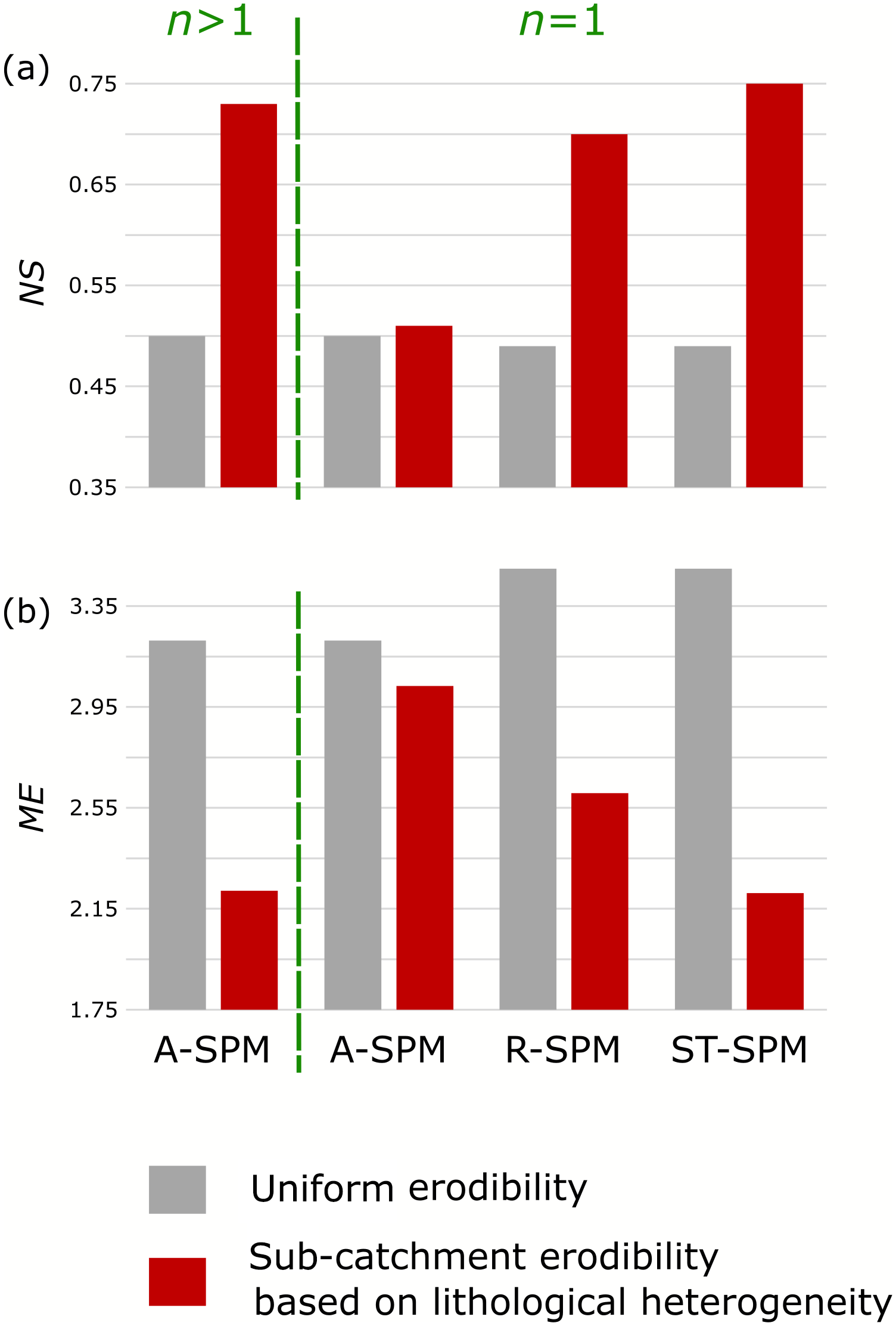
Figure 9Comparison of model performance for four selected river incision models. (a) Nash–Sutcliffe model efficiency (NS) for different model scenarios without (grey bars) or with (red bars) considering lithological heterogeneity; (b) the corresponding model error (ME). The A-SPM model scenario corresponds to the Area-Based Stream Power Model (see Fig. 7). It performs well when lithological heterogeneity is considered and all parameters are freely calibrated, resulting in a slope steepness exponent (n; see Eq. 1) of 1.63 (for a full overview of model parameters, see Table 4). In an A-SPM scenario in which n is fixed to 1, the model performance strongly deteriorates. In the R-SPM and ST-SPM models, n is fixed to the theoretically derived value of 1. The R-SPM model explicitly incorporates runoff variability (see Fig. 8a), and the ST-SPM model also includes an incision threshold (see Fig. 8b). Both models perform well when lithological heterogeneity is accounted for. Overall, the best model performance (highest NS and smallest ME) is obtained under the ST-SPM scenario in which lithological and runoff variability, as well as river incision thresholds, are considered.
5.4 Impact of runoff variability on long-term river incision rates
The A-SPM performs well in explaining ECRN when lithology is considered and n ≫1 (Fig. 9; high NS model efficiency, low ME). For n=1, the performance of the A-SPM is low. The result is consistent with earlier studies reporting n≫1 (e.g., DiBiase et al., 2010; Harel et al., 2016; Ouimet et al., 2009; Scherler et al., 2014), which Lague (2014) attributes to discharge variability and incision thresholds. We tested this hypothesis using the R-SPM and ST-SPM. Our results underscore the fact that the nonlinear relationship between ksn and ECRN can be attributed to the spatial variability of mean annual runoff. Figure 9 shows that the R-SPM (in which n is fixed to the theoretically obtained value of 1) performs better than an A-SPM when n is fixed to 1. In tectonically active regions, steep river reaches often spatially coincide with the edge of the mountain range over which mean annual rainfall rates are highest. Accordingly, if variations in runoff are not considered, the effects of orographic precipitation will be partly accommodated by a nonlinear relationship between river steepness and denudation rates. The R-SPM accounts for this effect but results in an underestimation of low river incision rates (Fig. 8a). Moreover, the model error (Fig. 9b) shows that the R-SPM does not perform as well as the A-SPM. In a final set of model runs, we apply the ST-SPM with the explicit simulation of a threshold, which improves model performance, especially for low denudation rates, resulting in an overall model error equal to the one obtained with the A-SPM with n≫1 (Fig. 9). This finding points to the potentially important role of thresholds for river incision to occur.
The model performance of the ST-SPM equals the performance of an empirical A-SPM with a slope exponent ≫1 (Fig. 9). Our interpretation is that (i) spatial variations in runoff and (ii) the incision thresholds are the causes of an observed nonlinear relation between ksn and ECRN. With a seemingly equal model performance, one could wonder what the benefit of the more complex ST-SPM model is over a simple, nonlinear A-SPM. The aim of using an ST-SPM is, however, beyond fitting observed denudation rates: we want to identify to what extent the system is forced by internal allogenic dynamics such as the presence of incision thresholds or external autogenic forces such as runoff variability. The use of the ST-SPM illustrated that both processes can be accounted for in a quantitative way so that future studies can explicitly consider their role when reconstructing past landscape response to external perturbations (e.g., climate change).
To further explore the interdependency between incision thresholds and spatial runoff variability, our approach can be applied to CRN datasets covering regions characterized by more pronounced rainfall gradients (e.g., in Chile: Carretier et al., 2018). Accounting for spatial variations in temporal discharge distributions (with k characterizing the stochastic flood occurrence) did not improve or deteriorate model performance (ST-SPM scenario 8 in Table 4). This is likely due to data limitations: the necessary data to characterize temporal variations in discharge within a given catchment over a timescale that is relevant for CRN-derived denudation rates are, at present, not available.
Our finding that spatial patterns in precipitation are related to river incision patterns corroborate findings in Hawaii (Ferrier et al., 2013), the Himalaya (Scherler et al., 2017) and in the Andes (Sorensen and Yanites, 2019). Sorensen and Yanites (2019) evaluated the role of latitudinal rainfall variability in the Andes in erosional efficiency using a set of numerical landscape evolution model runs. They show that erosion efficiency in tropical climates at low latitudes, where the Paute basin is located, is well captured by the spatial pattern of mean annual precipitation and thus runoff. At higher latitudes (25–50∘) where mean annual precipitation decreases but erosivity is still high due to the intensity of storms (Sorensen and Yanites, 2019), river erosivity is likely better captured by spatial patterns in storm magnitude and frequency.
Numerous studies report a nonlinear relationship between channel steepness and CRN-derived denudation rates. Based on the growing mechanistic understanding of river incision processes, this nonlinear relationship is often attributed to incision thresholds. Rainfall variability controls the frequency of river discharges that exceed incision thresholds. Although the dynamic interplay between stochastic runoff and incision thresholds theoretically results in a nonlinear relationship between channel steepness and denudation rates, coupling theory with field data has been challenging. We address this issue in the Paute basin where we scrutinize the relationship between CRN-derived denudation rates and river incision using three different stream power models. We show that lithological variability obscures the relationship between channel-steepness-based river incision and CRN-derived denudation rates.
In order to account for rock strength variability, which for the Paute basin is mainly ascribed to variations in lithological strength in the study area, we propose the use of an empirical lithological strength index that is based on the lithology and age of lithostratigraphic units. Including lithological variability in the models increases the correlation between river steepness and denudation rates and reveals a nonlinear relation, which we seek to explain using a stochastic-threshold SPM (ST-SPM). Using a downscaled version of a hydrological reanalysis dataset, we show that the combination of spatially varying runoff and incision thresholds explains the observed nonlinear relationship. We do not detect, however, an impact of temporal discharge patterns on river incision. We attribute this to the integration time of CRN data and response times of river longitudinal profiles, which extend beyond the timescales at which discharge distributions can be assumed to be stationary.
Our study shows the potential of an ST-SPM to infer regional and, potentially, continental to global differences in rainfall variability. However, we emphasize that its application needs to account for confounding environmental variables such as rock strength. Simplified process representation of stream-power-based incision models (e.g., lack of sediment–bedrock interactions) might explain part of the remaining scatter between predicted and measured denudation rates. However, residual analysis shows that most of the remaining scatter occurs in small transient catchments (up to 10 km2) where sporadic mass-wasting processes on hillslopes likely obscure the relation between measurements and predictions. Elucidating this relation further could potentially be fostered by dynamic numerical landscape evolutions models that explicitly simulate the coupling between transient river adjustment and hillslope response.
All data used in this paper are freely available from the referenced agencies. The hydrological data used in this paper were created in the framework of the Earth2ObserveWater Resource Reanalysis project (WRR2; Schellekens et al., 2017) and are available from 1979 to 2014. Specifically, we use the hydrological data calculated with the global water model WaterGAP3 (Water – Global Assessment and Prognosis: Alcamo et al., 2003; Döll et al., 2003) at a spatial resolution of 0.25 and a daily temporal resolution (http://www.earth2observe.eu, last access: 19 May 2020) (Schellekens et al., 2017). A high-resolution mean annual precipitation map (PRIDW) is calculated by downscaling the WaterGAP precipitation data (P) using a series of rain gauge observations (338 stations, 1990–2013) from the Ecuadorian national meteorological service (INAMHI; available from http://www.serviciometeorologico.gob.ec/biblioteca/, last access: 19 May 2020) (INAMHI, 2020). Topographic data are available from NASA (Farr et al., 2007). Lithological data are provided in the Supplement. Calculations were done in MATLAB using the Topo Toolbox Software (Schwanghart and Scherler, 2014).
The supplement related to this article is available online at: https://doi.org/10.5194/esurf-8-447-2020-supplement.
BC conceived the project in collaboration with VV, MVM and GG. BC performed the statistical analysis and took the lead in writing the paper. All authors contributed to shaping the research and analyses, as well as writing the paper.
The authors declare that they have no conflict of interest.
Benjamin Campforts received a postdoctoral grant from the Research Foundation
Flanders (FWO, reference number 12Z6518N). Gustavo E. Tenorio received a PhD grant
from ARES – the Académie de recherche et d'enseignement supérieur
de la Belgique – as part of the PRD research cooperation project
“Strengthening the scientific and technological capacities to implement
spatially integrated land and water management schemes adapted to local
socio-economic, cultural and physical settings”, as well as a grant from the
Secretaría de Educación Superior de Ciencia, Tecnología e
Innovación de la República del Ecuador. The article processing charges for this open-access
publication were covered by a Research Centre
of the Helmholtz Association.
This paper was edited by Simon Mudd and reviewed by two anonymous referees.
Aalto, R., Dunne, T., and Guyot, J. L.: Geomorphic Controls on Andean Denudation Rates, J. Geol., 114, 85–99, https://doi.org/10.1086/498101, 2006.
Abbühl, L. M., Norton, K. P., Jansen, J. D., Schlunegger, F., Aldahan, A., and Possnert, G.: Erosion rates and mechanisms of knickzone retreat inferred from 10Be measured across strong climate gradients on the northern and central Andes Western Escarpment, Earth Surf. Proc. Land., 36, 1464–1473, https://doi.org/10.1002/esp.2164, 2011.
Alcamo, J., Döll, P., Henrichs, T., Kaspar, F., Lehner, B., Rösch, T., and Siebert, S.: Development and testing of the WaterGAP 2 global model of water use and availability, Hydrolog. Sci. J., 48, 317–337, https://doi.org/10.1623/hysj.48.3.317.45290, 2003.
Anderson, R. S.: Evolution of the Santa Cruz Mountains, California, through tectonic growth and geomorphic decay, J. Geophys. Res., 99, 20161–20179, https://doi.org/10.1029/94JB00713, 1994.
Armitage, J. J., Whittaker, A. C., Zakari, M., and Campforts, B.: Numerical modelling of landscape and sediment flux response to precipitation rate change, Earth Surf. Dynam., 6, 77–99, https://doi.org/10.5194/esurf-6-77-2018, 2018.
Attal, M. and Lavé, J.: Pebble abrasion during fluvial transport: Experimental results and implications for the evolution of the sediment load along rivers, J. Geophys. Res., 114, F04023, https://doi.org/10.1029/2009JF001328, 2009.
Basabe, P.: Geologia Y Geotecnia, in Prevencion de Desastres Naturales en la Cuenca del Paute, Informe Final: Projecto PreCuPa. Swiss Disaster Relief Unit (SDR/CSS), Cuenca, Ecuador, 1–153, 1998.
Beck, H. E., van Dijk, A. I. J. M., de Roo, A., Dutra, E., Fink, G., Orth, R., and Schellekens, J.: Global evaluation of runoff from 10 state-of-the-art hydrological models, Hydrol. Earth Syst. Sci., 21, 2881–2903, https://doi.org/10.5194/hess-21-2881-2017, 2017.
Bendix, J., Rollenbeck, R., Göttlicher, D., and Cermak, J.: Cloud occurrence and cloud properties in Ecuador, Clim. Res., 30, 133–147, https://doi.org/10.3354/cr030133, 2006.
Bennett, G. L., Miller, S. R., Roering, J. J., and Schmidt, D. A.: Landslides, threshold slopes, and the survival of relict terrain in the wake of the Mendocino Triple Junction, Geology, 44, 363–366, https://doi.org/10.1130/G37530.1, 2016.
Bernhardt, A., Schwanghart, W., Hebbeln, D., Stuut, J.-B. W., and Strecker, M. R.: Immediate propagation of deglacial environmental change to deep-marine turbidite systems along the Chile convergent margin, Earth Planet. Sc. Lett., 473, 190–204, https://doi.org/10.1016/j.epsl.2017.05.017, 2017.
Binnie, S. A., Phillips, W. M., Summerfield, M. A., and Fifield, L. K.: Tectonic uplift, threshold hillslopes, and denudation rates in a developing mountain range, Geology, 35, 743–746, https://doi.org/10.1130/G23641A.1, 2007.
Bishop, P., Hoey, T. B., Jansen, J. D., and Artza, I. L.: Knickpoint recession rate and catchment area: the case of uplifted rivers in Eastern Scotland, Earth Surf. Proc. Land., 778, 767–778, https://doi.org/10.1002/esp.1191, 2005.
Blöthe, J. H., Korup, O., and Schwanghart, W.: Large landslides lie low: Excess topography in the Himalaya-Karakoram ranges, Geology, 43, 523–526, https://doi.org/10.1130/G36527.1, 2015.
Brocard, G. Y. and van der Beek, P. A.: Influence of incision rate, rock strength, and bedload supply on bedrock river gradients and valley-flat widths: Field-based evidence and calibrations from western Alpine rivers (southeast France), in Special Paper 398: Tectonics, Climate, and Landscape Evolution, 2398, 101–126, Geological Society of America, 2006.
Broeckx, J., Rossi, M., Lijnen, K., Campforts, B., Poesen, J., and Vanmaercke, M.: Landslide mobilization rates: A global analysis and model, Earth-Sci. Rev., 201, 102972, https://doi.org/10.1016/j.earscirev.2019.102972, 2020.
Burbank, D. W., Leland, J., Fielding, E., Anderson, R. S., Brozovic, N., Reid, M. R., and Duncan, C.: Bedrock incision, rock uplift and threshold hillslopes in the northwestern Himalayas, Nature, 379, 505–510, https://doi.org/10.1038/379505a0, 1996.
Campetella, C. M. and Vera, C. S.: The influence of the Andes mountains on the South American low-level flow, Geophys. Res. Lett., 29, 7-1–7-4, https://doi.org/10.1029/2002GL015451, 2002.
Campforts, B. and Govers, G.: Keeping the edge: A numerical method that avoids knickpoint smearing when solving the stream power law, J. Geophys. Res.-Earth, 120, 1189–1205, https://doi.org/10.1002/2014JF003376, 2015.
Campforts, B., Vanacker, V., Vanderborght, J., Baken, S., Smolders, E., and Govers, G.: Simulating the mobility of meteoric 10 Be in the landscape through a coupled soil-hillslope model (Be2D), Earth Planet. Sc. Lett., 439, 143–157, https://doi.org/10.1016/j.epsl.2016.01.017, 2016.
Campforts, B., Schwanghart, W., and Govers, G.: Accurate simulation of transient landscape evolution by eliminating numerical diffusion: the TTLEM 1.0 model, Earth Surf. Dynam., 5, 47–66, https://doi.org/10.5194/esurf-5-47-2017, 2017.
Carretier, S., Tolorza, V., Regard, V., Aguilar, G., Bermúdez, M. A., Martinod, J., Guyot, J. L., Hérail, G., and Riquelme, R.: Review of erosion dynamics along the major N-S climatic gradient in Chile and perspectives, Geomorphology, 300, 45–68, https://doi.org/10.1016/j.geomorph.2017.10.016, 2018.
Castelltort, S., Goren, L., Willett, S. D., Champagnac, J. D., Herman, F., and Braun, J.: River drainage patterns in the New Zealand Alps primarily controlled by plate tectonic strain, Nat. Geosci., 5, 744–748, https://doi.org/10.1038/ngeo1582, 2012.
Celleri, R., Willems, P., Buytaert, W., and Feyen, J.: Space–time rainfall variability in the Paute basin, Ecuadorian Andes, Hydrol. Process., 21, 3316–3327, https://doi.org/10.1002/hyp.6575, 2007.
Codilean, A. T., Munack, H., Cohen, T. J., Saktura, W. M., Gray, A., and Mudd, S. M.: OCTOPUS: an open cosmogenic isotope and luminescence database, Earth Syst. Sci. Data, 10, 2123–2139, https://doi.org/10.5194/essd-10-2123-2018, 2018.
Coulthard, T. J. and Van de Wiel, M. J.: Climate, tectonics or morphology: what signals can we see in drainage basin sediment yields?, Earth Surf. Dynam., 1, 13–27, https://doi.org/10.5194/esurf-1-13-2013, 2013.
Crave, A. and Davy, P.: A stochastic “precipiton” model for simulating erosion/sedimentation dynamics, Comput. Geosci., 27, 815–827, https://doi.org/10.1016/S0098-3004(00)00167-9, 2001.
Croissant, T. and Braun, J.: Constraining the stream power law: a novel approach combining a landscape evolution model and an inversion method, Earth Surf. Dynam., 2, 155–166, https://doi.org/10.5194/esurf-2-155-2014, 2014.
Cyr, A. J., Granger, D. E., Olivetti, V., and Molin, P.: Quantifying rock uplift rates using channel steepness and cosmogenic nuclide–determined erosion rates: Examples from northern and southern Italy, Lithosphere, 2, 188–198, https://doi.org/10.1130/L96.1, 2010.
Deal, E., Braun, J., and Botter, G.: Understanding the Role of Rainfall and Hydrology in Determining Fluvial Erosion Efficiency, J. Geophys. Res.-Earth, 123, 744–778, https://doi.org/10.1002/2017JF004393, 2018.
DiBiase, R. A. and Whipple, K. X.: The influence of erosion thresholds and runoff variability on the relationships among topography, climate, and erosion rate, J. Geophys. Res., 116, F04036, https://doi.org/10.1029/2011JF002095, 2011.
DiBiase, R. A., Whipple, K. X., Heimsath, A. M., and Ouimet, W. B.: Landscape form and millennial erosion rates in the San Gabriel Mountains, CA, Earth Planet. Sc. Lett., 289, 134–144, https://doi.org/10.1016/j.epsl.2009.10.036, 2010.
Dinku, T., Hailemariam, K., Maidment, R., Tarnavsky, E., and Connor, S.: Combined use of satellite estimates and rain gauge observations to generate high-quality historical rainfall time series over Ethiopia, Int. J. Climatol., 34, 2489–2504, https://doi.org/10.1002/joc.3855, 2014.
Döll, P., Kaspar, F., and Lehner, B.: A global hydrological model for deriving water availability indicators: model tuning and validation, J. Hydrol., 270, 105–134, https://doi.org/10.1016/S0022-1694(02)00283-4, 2003.
Dunai, T. J.: Scaling factors for production rates of in situ produced cosmogenic nuclides: a critical reevaluation, Earth Planet. Sc. Lett., 176, 157–169, https://doi.org/10.1016/S0012-821X(99)00310-6, 2000.
Egüez, A., Gaona, M., and Albán., A.: Mapa geológico de la República del Ecuador, Escala 1:1.000.000, Quito, 2017.
Farr, T. G., Rosen, P. A., Caro, E., Crippen, R., Duren, R., Hensley, S., Kobrick, M., Paller, M., Rodriguez, E., Roth, L., Seal, D., Shaffer, S., Shimada, J., Umland, J., Werner, M., Oskin, M., Burbank, D., and Alsdorf, D.: The Shuttle Radar Topography Mission, Rev. Geophys., 45, RG2004, https://doi.org/10.1029/2005RG000183, 2007.
Ferrier, K. L., Huppert, K. L., and Perron, J. T.: Climatic control of bedrock river incision, Nature, 496, 206–209, https://doi.org/10.1038/nature11982, 2013.
Finnegan, N. J., Hallet, B., Montgomery, D. R., Zeitler, P. K., Stone, J. O., Anders, A. M., and Yuping, L.: Coupling of rock uplift and river incision in the Namche Barwa-Gyala Peri massif, Tibet, Geol. Soc. Am. Bull., 120, 142–155, https://doi.org/10.1130/B26224.1, 2008.
Fisher, G. B., Amos, C. B., Bookhagen, B., Burbank, D. W., and Godard, V.: Channel widths, landslides, faults, and beyond: The new world order of high-spatial resolution Google Earth imagery in the study of earth surface processes, in: Google Earth and Virtual Visualizations in Geoscience Education and Research, Geological Society of America, 2012.
Fisher, G. B., Bookhagen, B., and Amos, C. B.: Channel planform geometry and slopes from freely available high-spatial resolution imagery and DEM fusion: Implications for channel width scalings, erosion proxies, and fluvial signatures in tectonically active landscapes, Geomorphology, 194, 46–56, https://doi.org/10.1016/j.geomorph.2013.04.011, 2013.
Garcia-Castellanos, D. and Jiménez-Munt, I.: Topographic Evolution and Climate Aridification during Continental Collision: Insights from Computer Simulations, edited by: N. Houlie, PLoS One, 10, e0132252, https://doi.org/10.1371/journal.pone.0132252, 2015.
Gasparini, N. M. and Whipple, K. X.: Diagnosing climatic and tectonic controls on topography: Eastern flank of the northern Bolivian Andes, Lithosphere, 6, 230–250, https://doi.org/10.1130/L322.1, 2014.
Goren, L.: A theoretical model for fluvial channel response time during time-dependent climatic and tectonic forcing and its inverse applications, Geophys. Res. Lett., 43, 10753–10763, https://doi.org/10.1002/2016GL070451, 2016.
Goren, L., Fox, M., and Willett, S. D.: Tectonics from fluvial topography using formal linear inversion: Theory and applications to the Inyo Mountains, California, J. Geophys. Res.-Earth, 119, 1651–1681, https://doi.org/10.1002/2014JF003079, 2014.
Guns, M. and Vanacker, V.: Forest cover change trajectories and their impact on landslide occurrence in the tropical Andes, Environ. Earth Sci., 70, 2941–2952, https://doi.org/10.1007/s12665-013-2352-9, 2013.
Guns, M. and Vanacker, V.: Shifts in landslide frequency-area distribution after forest conversion in the tropical Andes, Anthropocene, 6, 75–85, https://doi.org/10.1016/j.ancene.2014.08.001, 2014.
Harel, M. M.-A., Mudd, S. M., and Attal, M.: Global analysis of the stream power law parameters based on worldwide 10 Be denudation rates, Geomorphology, 268, 184–196, https://doi.org/10.1016/j.geomorph.2016.05.035, 2016.
Hay, W. W., Sloan Ii, J. L., and Wold, C. N.: Mass/Age Distribution and Composition of Sediments on the Ocean Floor and the Global Rate of Sediment Subduction, J. Geophys. Res., 93940, 933–14, https://doi.org/10.1029/JB093iB12p14933, 1988.
Herman, F., Beyssac, O., Brughelli, M., Lane, S. N., Leprince, S., Adatte, T., Lin, J. Y. Y., Avouac, J.-P., and Cox, S. C.: Erosion by an Alpine glacier, Science, 350, 193–195, https://doi.org/10.1126/science.aab2386, 2015.
Hobley, D. E. J., Adams, J. M., Nudurupati, S. S., Hutton, E. W. H., Gasparini, N. M., Istanbulluoglu, E., and Tucker, G. E.: Creative computing with Landlab: an open-source toolkit for building, coupling, and exploring two-dimensional numerical models of Earth-surface dynamics, Earth Surf. Dynam., 5, 21–46, https://doi.org/10.5194/esurf-5-21-2017, 2017.
Horton, B. K.: Sedimentary record of Andean mountain building, Earth-Sci. Rev., 178, 279–309, https://doi.org/10.1016/j.earscirev.2017.11.025, 2018.
Howard, A. D.: A detachment limited model of drainage basin evolution, Water Resour. Res., 30, 2261–2285, https://doi.org/10.1029/94WR00757, 1994.
Hungerbühler, D., Steinmann, M., Winkler, W., Seward, D., Egüez, A., Peterson, D. E., Helg, U., and Hammer, C.: Neogene stratigraphy and Andean geodynamics of southern Ecuador, Earth-Sci. Rev., 57, 75–124, https://doi.org/10.1016/S0012-8252(01)00071-X, 2002.
Hurst, M. D., Mudd, S. M., Walcott, R., Attal, M., and Yoo, K.: Using hilltop curvature to derive the spatial distribution of erosion rates, J. Geophys. Res.-Earth, 117, F02017, https://doi.org/10.1029/2011JF002057, 2012.
INAMHI – Instituto Nacional de Meteorología e Hidrología: Ecuadorian national meteorological service, Anuario Meteorológico [Annual reports from 1990–2013], available at: http://www.serviciometeorologico.gob.ec/biblioteca/, last access: 19 May 2020.
Jelinski, N. A., Campforts, B., Willenbring, J. K., Schumacher, T. E., Li, S., Lobb, D. A., Papiernik, S. K., and Yoo, K.: Meteoric Beryllium-10 as a Tracer of Erosion Due to Postsettlement Land Use in West-Central Minnesota, USA, J. Geophys. Res.-Earth, 124, 874–901, https://doi.org/10.1029/2018JF004720, 2019.
Jerolmack, D. J. and Paola, C.: Shredding of environmental signals by sediment transport, Geophys. Res. Lett., 37, 1–5, https://doi.org/10.1029/2010GL044638, 2010.
Kirby, E. and Ouimet, W.: Tectonic geomorphology along the eastern margin of Tibet: insights into the pattern and processes of active deformation adjacent to the Sichuan Basin, Geol. Soc. Lond. Spec. Publ., 353, 165, https://doi.org/10.1144/sp353.9, 2011.
Kirby, E. and Whipple, K. X.: Expression of active tectonics in erosional landscapes, J. Struct. Geol., 44, 54–75, https://doi.org/10.1016/j.jsg.2012.07.009, 2012.
Kirchner, J. W., Finkel, R. C., Riebe, C. S., Granger, D. E., Clayton, J. L., King, J. G., and Megahan, W. F.: Mountain erosion over 10 yr, 10 k.y., and 10 m.y. time scales, Geology, 29, 591, https://doi.org/10.1130/0091-7613(2001)029<0591:MEOYKY>2.0.CO;2, 2001.
Kober, F., Ivy-Ochs, S., Schlunegger, F., Baur, H., Kubik, P. W., and Wieler, R.: Denudation rates and a topography-driven rainfall threshold in northern Chile: Multiple cosmogenic nuclide data and sediment yield budgets, Geomorphology, 83, 97–120, https://doi.org/10.1016/j.geomorph.2006.06.029, 2007.
Kober, F., Zeilinger, G., Hippe, K., Marc, O., Lendzioch, T., Grischott, R., Christl, M., Kubik, P. W., and Zola, R.: Tectonic and lithological controls on denudation rates in the central Bolivian Andes, Tectonophysics, 657, 230–244, https://doi.org/10.1016/j.tecto.2015.06.037, 2015.
Korup, O., Clague, J. J., Hermanns, R. L., Hewitt, K., Strom, A. L., and Weidinger, J. T.: Giant landslides, topography, and erosion, Earth Planet. Sci. Lett., 261, 578–589, https://doi.org/10.1016/j.epsl.2007.07.025, 2007.
Lague, D.: The stream power river incision model: evidence, theory and beyond, Earth Surf. Proc. Land., 39, 38–61, https://doi.org/10.1002/esp.3462,
2014.
Lague, D., Hovius, N., and Davy, P.: Discharge, discharge variability, and the bedrock channel profile, J. Geophys. Res.-Earth, 110, https://doi.org/10.1029/2004JF000259, 2005.
Larsen, I. J., Montgomery, D. R., and Korup, O.: Landslide erosion controlled by hillslope material, Nat. Geosci., 3, 247–251, https://doi.org/10.1038/ngeo776, 2010.
Lavé, J. and Avouac, J. P.: Fluvial incision and tectonic uplift across the Himalayas of central Nepal, J. Geophys. Res.-Sol. Ea., 106, 26561–26591, https://doi.org/10.1029/2001JB000359, 2001.
Leopold, L. B. and Maddock, T.: The hydraulic geometry of stream channels and some physiographic implications, US Government Printing Office, 1953.
Mandal, S. K., Lupker, M., Burg, J.-P., Valla, P. G., Haghipour, N., and Christl, M.: Spatial variability of 10Be-derived erosion rates across the southern Peninsular Indian escarpment: A key to landscape evolution across passive margins, Earth Planet. Sc. Lett., 425, 154–167, https://doi.org/10.1016/j.epsl.2015.05.050, 2015.
Manz, B., Buytaert, W., Zulkafli, Z., Lavado, W., Willems, B., Robles, L. A., and Rodríguez-Sánchez, J.-P.: High-resolution satellite-gauge merged precipitation climatologies of the Tropical Andes, J. Geophys. Res.-Atmos., 121, 1190–1207, https://doi.org/10.1002/2015JD023788, 2016.
Meyer-Peter, E. and Müller, R.: Formulas for Bed-Load Transport, Proc. Int. Assoc. Hydraul. Struct. Researach – Second Meet. Stock. Sweeden, 39–65, doi:1948-06-07, 1948.
Molina, A., Govers, G., Vanacker, V., Poesen, J., Zeelmaekers, E., and Cisneros, F.: Runoff generation in a degraded Andean ecosystem: Interaction of vegetation cover and land use, CATENA, 71, 357–370, https://doi.org/10.1016/j.catena.2007.04.002, 2007.
Molnar, P., Anderson, R. S., Kier, G., and Rose, J.: Relationships among probability distributions of stream discharges in floods, climate, bed load transport, and river incision, J. Geophys. Res., 111, F02001, https://doi.org/10.1029/2005JF000310, 2006.
Molnar, P., Anderson, R. S., and Anderson, S. P.: Tectonics, fracturing of rock, and erosion, J. Geophys. Res., 112, F03014, https://doi.org/10.1029/2005JF000433, 2007.
Montgomery, D. R. and Brandon, M. T.: Topographic controls on erosion rates in tectonically active mountain ranges, Earth Planet. Sc. Lett., 201, 481–489, https://doi.org/10.1016/S0012-821X(02)00725-2, 2002.
Mora, D. E., Campozano, L., Cisneros, F., Wyseure, G., and Willems, P.: Climate changes of hydrometeorological and hydrological extremes in the Paute basin, Ecuadorean Andes, Hydrol. Earth Syst. Sci., 18, 631–648, https://doi.org/10.5194/hess-18-631-2014, 2014.
Muñoz, P., Orellana-Alvear, J., Willems, P., and Célleri, R.: Flash-Flood Forecasting in an Andean Mountain Catchment–Development of a Step-Wise Methodology Based on the Random Forest Algorithm, Water, 10, 1519, https://doi.org/10.3390/w10111519, 2018.
Nash, J. E. and Sutcliffe, J. V.: River flow forecasting through conceptual models part I – A discussion of principles, J. Hydrol., 10, 282–290, https://doi.org/10.1016/0022-1694(70)90255-6, 1970.
Nearing, M. A., Wei, H., Stone, J. J., Pierson, F. B., Spaeth, K. E., Weltz, M. A., Flanagan, D. C., and Hernandez, M.: A Rangeland Hydrology and Erosion Model, T. ASABE, 54, 901–908, https://doi.org/10.13031/2013.37115, 2011.
Nibourel, L., Herman, F., Cox, S. C., Beyssac, O., and Lavé, J.: Provenance analysis using Raman spectroscopy of carbonaceous material: A case study in the Southern Alps of New Zealand, J. Geophys. Res.-Earth, 120, 2056–2079, https://doi.org/10.1002/2015JF003541, 2015.
Niemi, N. A., Oskin, M., Burbank, D. W., Heimsath, A. M., and Gabet, E. J.: Effects of bedrock landslides on cosmogenically determined erosion rates, Earth Planet. Sc. Lett., 237, 480–498, https://doi.org/10.1016/j.epsl.2005.07.009, 2005.
Norton, K. P. and Vanacker, V.: Effects of terrain smoothing on topographic shielding correction factors for cosmogenic nuclide-derived estimates of basin-averaged denudation rates, Earth Surf. Proc. Land., 34, 145–154, https://doi.org/10.1002/esp.1700, 2009.
Ouimet, W. B., Whipple, K. X., and Granger, D. E.: Beyond threshold hillslopes: Channel adjustment to base-level fall in tectonically active mountain ranges, Geology, 37, 579–582, https://doi.org/10.1130/G30013A.1, 2009.
Petersen, M. D., Harmsen, S. C., Jaiswal, K. S., Rukstales, K. S., Luco, N., Haller, K. M., Mueller, C. S., and Shumway, A. M.: Seismic Hazard, Risk, and Design for South America, B. Seismol. Soc. Am., 108, 781–800, https://doi.org/10.1785/0120170002, 2018.
Portenga, E. W. and Bierman, P. R.: Understanding Earth's eroding surface with 10Be, GSA Today, 21, 4–10, https://doi.org/10.1130/G111A.1, 2011.
Reusser, L., Bierman, P., and Rood, D.: Quantifying human impacts on rates of erosion and sediment transport at a landscape scale, Geology, 43, 171–174, https://doi.org/10.1130/G36272.1, 2015.
Riebe, C. S., Kirchner, J. W., Granger, D. E., and Finkel, R. C.: Strong tectonic and weak climatic control of long-term chemical weathering rates, Geology, 29, 511, https://doi.org/10.1130/0091-7613(2001)029<0511:STAWCC>2.0.CO;2, 2001.
Roberts, G. G. and White, N.: Estimating uplift rate histories from river profiles using African examples, J. Geophys. Res., 115, B02406, https://doi.org/10.1029/2009JB006692, 2010.
Roering, J. J., Kirchner, J. W., and Dietrich, W. E.: Evidence for nonlinear, diffusive sediment transport on hillslopes and implications for landscape morphology, Water Resour. Res., 35, 853–870, https://doi.org/10.1029/1998WR900090, 1999.
Romans, B. W., Castelltort, S., Covault, J. A., Fildani, A., and Walsh, J. P.: Environmental signal propagation in sedimentary systems across timescales, Earth-Sci. Rev., 153, 7–29, https://doi.org/10.1016/j.earscirev.2015.07.012, 2016.
Royden, L. and Perron, J. T.: Solutions of the stream power equation and application to the evolution of river longitudinal profiles, J. Geophys. Res.-Earth, 118, 497–518, https://doi.org/10.1002/jgrf.20031, 2013.
Sadler, P. M.: Sediment Accumulation Rates and the Completeness of Stratigraphic Sections, J. Geol., 89, 569–584, https://doi.org/10.1086/628623, 1981.
Safran, E. B., Bierman, P. R., Aalto, R., Dunne, T., Whipple, K. X., and Caffee, M.: Erosion rates driven by channel network incision in the Bolivian Andes, Earth Surf. Proc. Land., 30, 1007–1024, https://doi.org/10.1002/esp.1259, 2005.
Schaller, M., von Blanckenburg, F., Hovius, N., and Kubik, P. W.: Large-scale erosion rates from in situ-produced cosmogenic nuclides in European river sediments, Earth Planet. Sc. Lett., 188, 441–458, https://doi.org/10.1016/S0012-821X(01)00320-X, 2001.
Schaller, M., von Blanckenburg, F., Veldkamp, A., Tebbens, L. A., Hovius, N. and Kubik, P. W.: A 30 000 yr record of erosion rates from cosmogenic 10Be in Middle European river terraces, Earth Planet. Sc. Lett., 204, 307–320, https://doi.org/10.1016/S0012-821X(02)00951-2, 2002.
Schellekens, J., Dutra, E., Martínez-de la Torre, A., Balsamo, G., van Dijk, A., Sperna Weiland, F., Minvielle, M., Calvet, J.-C., Decharme, B., Eisner, S., Fink, G., Flörke, M., Peßenteiner, S., van Beek, R., Polcher, J., Beck, H., Orth, R., Calton, B., Burke, S., Dorigo, W., and Weedon, G. P.: A global water resources ensemble of hydrological models: the eartH2Observe Tier-1 dataset, Earth Syst. Sci. Data, 9, 389–413, https://doi.org/10.5194/essd-9-389-2017, 2017.
Scherler, D., Bookhagen, B., and Strecker, M. R.: Tectonic control on 10 Be-derived erosion rates in the Garhwal Himalaya, India, J. Geophys. Res.-Earth, 119, 83–105, https://doi.org/10.1002/2013JF002955, 2014.
Scherler, D., DiBiase, R. A., Fisher, G. B., and Avouac, J.-P.: Testing monsoonal controls on bedrock river incision in the Himalaya and Eastern Tibet with a stochastic-threshold stream power model, J. Geophys. Res.-Earth, 122, 1389–1429, https://doi.org/10.1002/2016JF004011, 2017.
Schmidt, K. M. and Montgomery, D. R.: Limits to Relief, Science, 270, 617–620, https://doi.org/10.1126/science.270.5236.617, 1995.
Schwanghart, W. and Scherler, D.: Short Communication: TopoToolbox 2 – MATLAB-based software for topographic analysis and modeling in Earth surface sciences, Earth Surf. Dynam., 2, 1–7, https://doi.org/10.5194/esurf-2-1-2014, 2014.
Schwanghart, W., Ryan, M., and Korup, O.: Topographic and Seismic Constraints on the Vulnerability of Himalayan Hydropower, Geophys. Res. Lett., 45, 8985–8992, https://doi.org/10.1029/2018GL079173, 2018.
Shobe, C. M., Tucker, G. E., and Barnhart, K. R.: The SPACE 1.0 model: a Landlab component for 2-D calculation of sediment transport, bedrock erosion, and landscape evolution, Geosci. Model Dev., 10, 4577–4604, https://doi.org/10.5194/gmd-10-4577-2017, 2017.
Shobe, C. M., Tucker, G. E., and Rossi, M. W.: Variable-Threshold Behavior in Rivers Arising From Hillslope-Derived Blocks, J. Geophys. Res.-Earth, 123, 1931–1957, https://doi.org/10.1029/2017JF004575, 2018.
Sklar, L. and Dietrich, W. E.: River longitudinal profiles and bedrock incision models: Stream power and the influence of sediment supply, 237–260., 1998.
Snyder, N. P., Whipple, K. X., Tucker, G. E., and Merritts, D. J.: Landscape response to tectonic forcing: Digital elevation model analysis of stream profiles in the Mendocino triple junction region, northern California, Geol. Soc. Am. Bull., 112, 1250–1263, https://doi.org/10.1130/0016-7606(2000)112<1250:LRTTFD>2.3.CO;2, 2000.
Snyder, N. P., Whipple, K. X., Tucker, G. E., and Merritts, D. J.: Importance of a stochastic distribution of floods and erosion thresholds in the bedrock river incision problem, J. Geophys. Res.-Sol. Ea., 108, 2388, https://doi.org/10.1029/2001JB001655, 2003.
Sorensen, C. S. and Yanites, B. J.: Latitudinal trends in modern fluvial erosional efficiency along the Andes, Geomorphology, 329, 170–183, https://doi.org/10.1016/j.geomorph.2018.12.030, 2019.
Spikings, R., Winkler, W., Seward, D., and Handler, R.: Along-strike variations in the thermal and tectonic response of the continental Ecuadorian Andes to the collision with heterogeneous oceanic crust, Earth Planet. Sc. Lett., 186, 57–73, https://doi.org/10.1016/S0012-821X(01)00225-4, 2001.
Spikings, R. A. and Crowhurst, P. V.: (U–Th) ∕ He thermochronometric constraints on the late Miocene–Pliocene tectonic development of the northern Cordillera Real and the Interandean Depression, Ecuador, J. South Am. Earth Sci., 17, 239–251, https://doi.org/10.1016/j.jsames.2004.07.001, 2004.
Spikings, R. A., Crowhurst, P. V., Winkler, W., and Villagomez, D.: Syn- and post-accretionary cooling history of the Ecuadorian Andes constrained by their in-situ and detrital thermochronometric record, J. South Am. Earth Sci., 30, 121–133, https://doi.org/10.1016/j.jsames.2010.04.002, 2010.
Steinmann, M., Hungerbühler, D., Seward, D., and Winkler, W.: Neogene tectonic evolution and exhumation of the southern Ecuadorian Andes: a combined stratigraphy and fission-track approach, Tectonophysics, 307, 255–276, https://doi.org/10.1016/S0040-1951(99)00100-6, 1999.
Stock, J. D. and Montgomery, D. R.: Geologic constraints on bedrock river incision using the stream power law, J. Geophys. Res., 104, 4983, https://doi.org/10.1029/98JB02139, 1999.
Tofelde, S., Duesing, W., Schildgen, T. F., Wickert, A. D., Wittmann, H., Alonso, R. N., and Strecker, M.: Effects of deep-seated versus shallow hillslope processes on cosmogenic 10Be concentrations in fluvial sand and gravel, Earth Surf. Proc. Land., 43, 3086–3098, https://doi.org/10.1002/esp.4471, 2018.
Tucker, G. E.: Drainage basin sensitivity to tectonic and climatic forcing: Implications of a stochastic model for the role of entrainment and erosion thresholds, Earth Surf. Proc. Land., 29, 185–205, https://doi.org/10.1002/esp.1020, 2004.
Tucker, G. E. and Bras, R. L.: A stochastic approach to modeling the role of rainfall variability in drainage basin evolution, Water Resour. Res., 36, 1953–1964, https://doi.org/10.1029/2000WR900065, 2000.
Tucker, G. E. and Hancock, G. R.: Modelling landscape evolution, Earth Surf. Proc. Land., 35, 28–50, https://doi.org/10.1002/esp.1952, 2010.
Vanacker, V., von Blanckenburg, F., Govers, G., Molina, A., Poesen, J., Deckers, J., and Kubik, P.: Restoring dense vegetation can slow mountain erosion to near natural benchmark levels, Geology, 35, 303–306, https://doi.org/10.1130/G23109A.1, 2007.
Vanacker, V., von Blanckenburg, F., Govers, G., Molina, A., Campforts, B., and Kubik, P. W.: Transient river response, captured by channel steepness and its concavity, Geomorphology, 228, 234–243, https://doi.org/10.1016/j.geomorph.2014.09.013, 2015.
Vanacker, V., Guns, M., Clapuyt, F., Balthazar, V., Tenorio, G., and Molina, A.: Spatio-temporal patterns of landslides and erosion in tropical andean catchments, Pirineos a J. Mt. Ecol.,75, https://doi.org/10.3989/pirineos.2020.175001, in press, 2020.
Venditti, J. G., Li, T., Deal, E., Dingle, E., and Church, M.: Struggles with stream power: Connecting theory across scales, Geomorphology, 106817, https://doi.org/10.1016/j.geomorph.2019.07.004, in press, 2019.
Whipple, K. X.: Fluvial landscape response time: How plausible is steady-state denudation?, Am. J. Sci., 301, 313–325, https://doi.org/10.2475/ajs.301.4-5.313, 2001.
Whipple, K. X. and Tucker, G. E.: Dynamics of the stream-power river incision model: Implications for height limits of mountain ranges, landscape response timescales, and research needs, J. Geophys. Res.-Sol. Ea., 104, 17661–17674, https://doi.org/10.1029/1999JB900120, 1999.
Whipple, K. X., Kirby, E., and Brocklehurst, S. H.: Geomorphic limits to climate-induced increases in topographic relief, Nature, 401, 39–43, https://doi.org/10.1038/43375, 1999.
Whipple, K. X., Hancock, G. S., and Anderson, R. S.: River incision into bedrock: Mechanics and relative efficacy of plucking, abrasion, and cavitation, Geol. Soc. Am. Bull., 112, 490–503, https://doi.org/10.1130/0016-7606(2000)112<490:RIIBMA>2.0.CO;2, 2000.
Whipple, K. X., DiBiase, R. A., and Crosby, B. T.: 9.28 Bedrock Rivers, in Treatise on Geomorphology, vol. 9, edited by: Shroder, J. F., Elsevier, San Diego, 550–573, 2013.
Whittaker, A. C. and Boulton, S. J.: Tectonic and climatic controls on knickpoint retreat rates and landscape response times, J. Geophys. Res., 117, F02024, https://doi.org/10.1029/2011JF002157, 2012.
Wobus, C., Whipple, K. X., Kirby, E., Snyder, N., Johnson, J., Spyropolou, K., Crosby, B., and Sheehan, D.: Tectonics from topography: Procedures, promise, and pitfalls, in Tectonics, Climate, and Landscape Evolution, 398, Geological Society of America, 55–74, 2006.
Yanites, B. J., Tucker, G. E., and Anderson, R. S.: Numerical and analytical models of cosmogenic radionuclide dynamics in landslide-dominated drainage basins, J. Geophys. Res., 114, F01007, https://doi.org/10.1029/2008JF001088, 2009.