the Creative Commons Attribution 4.0 License.
the Creative Commons Attribution 4.0 License.
 | 12 Jun 2020
Identifying sediment transport mechanisms from grain size–shape distributions, applied to aeolian sediments
Johannes Albert van Hateren
Unze van Buuren
Sebastiaan Martinus Arens
Ronald Theodorus van Balen
Maarten Arnoud Prins
The way in which sediment is transported (creep, saltation, suspension), is traditionally interpreted from grain size distribution characteristics. However, the grain size range associated with transitions from one transport mode to the other is highly variable because it depends on the amount of transport energy available. In this study we present a novel methodology for determination of the sediment transport mode based on grain size and shape data from dynamic image analysis. The data are integrated into grain size–shape distributions, and primary components are determined using endmember modelling. In real-world datasets, primary components can be interpreted in terms of different transport mechanisms and/or sediment sources. Accuracy of the method is assessed using artificial datasets with known primary components that are mixed in known proportions. The results show that the proposed technique accurately identifies primary components, with the exception of those primary components that only form minor contributions to the samples (highly mixed components).
The new method is tested on sediment samples from an active aeolian system in the Dutch coastal dunes. Aeolian transport processes and geomorphology of these type of systems are well known and can therefore be linked to the spatial distribution of endmembers to assess the physical significance of the method's output. The grain size–shape distributions of the aeolian dune dataset are unmixed into three primary components. The spatial distribution of these components is constrained by geomorphology and reflects the three dominant aeolian transport processes known to occur along a beach–dune transect: bedload on the beach and in notches that were dug by man through the shore-parallel foredune ridge, modified saltation on the windward and leeward slope of the intact foredune, and suspension in the vegetated hinterland. The three transport modes are characterised by distinctly different trends in grain shape with grain size: with increasing size, bedload shows a constant grain regularity, modified saltation a minor decrease in grain regularity, and suspension a strong decrease in grain regularity. These trends, or in other words, the shape of the grain size–shape distributions, can be used to determine the transport mode responsible for an aeolian sediment deposit. Results of the method are therefore less ambiguous than those of traditional grain size distribution endmember modelling, especially if multiple transport modes occur or if primary components overlap in terms of grain size but differ in grain shape.
- Article
(40377 KB) - Full-text XML
- BibTeX
- EndNote


Clastic sediment records are generally complex mixtures of grains due to variability in provenance; conditions in the source and sink areas (climate, tectonics); and sorting during entrainment, transport, and deposition. One of the greatest challenges in sedimentology is to reconstruct signals of climate, tectonics, and provenance from the sedimentary record (e.g. Garzanti et al., 2007; Métivier et al., 1998; Prins and Weltje, 1999a; Zhang et al., 2016). These reconstructions are improved when the mixed sedimentary record is unmixed into its primary constituent components (Weltje and Prins, 2007), a procedure which is also termed endmember modelling. Various endmember modelling algorithms are used in sedimentology (e.g. Dietze et al., 2012; Heslop et al., 2007; Paterson and Heslop, 2015; Weltje, 1997; Yu et al., 2016; Zhang et al., 2018). Although the algorithms are capable of unmixing different types of data, they are commonly used on grain size distribution data (e.g. Dietze et al., 2014; Liu et al., 2016; Stuut et al., 2002) and mineralogical data (Itambi et al., 2009; Weltje, 1995).
There are, however, at least two issues that complicate inferences based on single-property (size or mineralogy) endmember modelling. First, sediment behaviour during uptake, transport, and deposition is dictated by three grain properties: size, shape, and density (mineralogy) (Winkelmolen, 1971). Therefore, single-property endmember modelling results are prone to noise from variability in the other two grain properties. The second issue is that the characterisation of sediment transport modes by their grain size distribution alone produces ambiguous results: the grain size range associated with the transitions between transport modes (surface creep, saltation, and suspension) depends on the amount of transport energy available and is therefore highly variable (Visher, 1969). However, accurate identification of the transport mode is essential to a valid interpretation of sedimentary records, since the transport modes sort sediment grains differently during transport and are associated with different transport velocities and distances.
In addition to sorting on grain size, sediment transport modes also sort shape in different ways. The role of particle shape in aeolian transport is highlighted because the method presented in the current paper is tested on an aeolian system. Studies on the influence of particle shape on surface creep are sparse. Eisma (1965) inferred that it is likely that surface creep favours spherical grains because these roll more easily. There are contradicting views regarding shape sorting during saltation: spherical grains bounce higher (Eisma, 1965) and further (MacCarthy and Huddle, 1938) and thus travel faster than non-spherical grains. However, they are also more difficult to entrain (Winkelmolen, 1971). Likewise, studies on shape sorting in saltating transport under natural conditions obtained contradictive results: some publications observed an increase in sphericity with transport distance (MacCarthy and Huddle, 1938; Mazzullo et al., 1986), and others observed a decrease (Eisma, 1965; Winkelmolen, 1971). This is further complicated by the fact that inter-grain collision during (aeolian) saltation effectively rounds grains over longer distances (Kuenen, 1960). During transport in suspension, settling velocity is the dominant sorting parameter (McCave, 2008; Pye, 1994). Settling velocity is higher for more spherical and regularly shaped grains (e.g. Dietrich, 1982; Komar and Reimers, 1978; Wadell, 1934). Hence, in a suspended population of grains, larger grains are expected to be more irregularly shaped than smaller ones to remain below the fall velocity threshold for suspended transport. For example, Shang et al. (2018) observed that elongation increases with increasing size in Chinese loess. This decrease in grain regularity with increasing size should lead to a characteristic size–shape trend of suspended sediment that is different from that of sediment transported as bedload; using grain shape in addition to grain size is therefore a promising approach to determine transport modes with less ambiguity.
In this study we outline a new method for determination of sediment transport processes involving (1) the integration of grain size and shape data into size–shape distributions (e.g. Itoh and Wanibe, 1991) and (2) endmember modelling on these distributions. To determine the accuracy of the method, it is first tested on artificial grain size–shape datasets with known endmembers and known endmember mixing proportions. Subsequently, the method is applied to an active aeolian system in the Dutch coastal dunes (Ruessink et al., 2018). Aeolian transport processes and geomorphology of these type of systems are relatively well constrained (Arens et al., 2002) and can therefore be linked to the spatial distribution of endmembers to assess the physical significance of the method's output. The real-world dataset is also used to compare results of unmixing of size–shape distributions to results of traditional unmixing based on grain size distributions.
2.1 Aeolian dune dataset
The fieldwork area for our dataset is situated south of the town IJmuiden in a coastal dune region named Nationaal Park Zuid-Kennemerland (Fig. 1a and b). In 2013, five notches were dug through the shore-parallel foredune ridge to promote aeolian activity and dune migration (Fig. 1b). The notches are roughly orientated along the dominant wind direction: west–southwest to east–northeast. Parabolic dunes have developed at the downwind end of the notches, and large volumes of sand have been blown land-inward. From 2013 to 2016, approximately 87×103 m3 of sand was transported land-inward, 55 % of which was derived from the beach and 45 % from erosion of the notches (Ruessink et al., 2018). Further land-inward, vegetation has been removed from fossil parabolic dunes to stimulate reactivation of dunes (Fig. 1b).

Figure 1Fieldwork area in the coastal dunes of the Nationaal Park Zuid-Kennemerland. Panel (a) shows the general location of the study area. Panel (b) displays the locations of surface samples and sediment traps. Panel (c) covers the same area and shows subregions based on geomorphologic features. Aerial photograph © PDOK.nl, 2017.
In order to assess the physical meaning of results from the new method, we divided the study area into its five main geomorphologic features (Fig. 1c): (1) the beach, which acts as a sediment source for aeolian transport when dry, (2) the foredune, on which marram grass (partly) impedes aeolian bedload transport (near the crest, aeolian suspension and modified saltation are stimulated through increased wind velocities and high turbulence; Arens et al., 2002), (3) the notches, which enable bedload transport towards the sand lobes that prograde into the vegetated hinterland (Ruessink et al., 2018), (4) the vegetated hinterland, where lower wind velocities and vegetation prevent bedload transport (Arens et al., 2002), and (5) the parabolic dunes that were reactivated by removal of the vegetation cover. These dunes may form an additional source for the sediment flux in the hinterland (Arens et al., 2013).
Table 1Wind conditions and sampling periods of the sediment-trap samples. Sediment-trap names are in reference to Fig. 1b. Meteorological data were obtained from weather station IJmuiden, 3.5 km north of the fieldwork area. Dates are listed in the format dd/mm/yyyy.
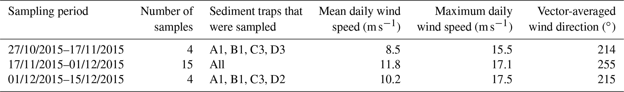
In April 2017, shallow surface samples were obtained from one of the bare notches (n=12) and from an undisturbed part of the foredune ridge (n=18) (Fig. 1b). Based on available flux data from sediment traps (not shown here), deposition rates landward from sediment-trap row A (or perhaps B) are insufficient to sample recently transported material from the surface (Fig. 1b). Samples from sediment traps (n=23) are therefore used to study the inland area. The traps are based on a design by Leatherman (1978) and consist of an 80 cm PVC pipe with a middle height of approximately 1.5 m a.g.l. (Fig. A1 in the Appendix). Their opening is oriented into the dominant southwestern wind direction. At the back of the pipe a mesh with openings of 106 µm lets air and smaller particles through while trapping particles larger than 106 µm. Three time intervals characterised by high flux rates (“storm events”) were sampled from the sediment traps (Table 1). Together, the sediment-trap samples and surface samples form the aeolian dune dataset (Van Hateren, 2019).
2.2 Dynamic image analysis
Sediment samples of approximately 2 g are pre-treated with 5 mL H2O2 to remove organics, 5 mL HCl (10 mL if shell fragments are abundant) to remove carbonates, and 300 mg Na4P2O7⋅10H2O to disperse charged particles (Konert and Vandenberghe, 1997). Size and shape data are based on images of the grains obtained using a Sympatec QICPIC dynamic image analyser (Fig. 2a). The image analyser is set up using a cuvette with 2 mm aperture. Pre-treated samples are sieved through a 1.6 mm mesh to protect the glass walls of this cuvette, thus limiting the maximum measurable grain size to 1600 µm. This is not of concern for the dune sands studied here, which show a maximum grain size of approximately 700 µm. The sediment samples are subsequently suspended in degassed water using a stirrer and pumped repeatedly through the cuvette for 10 min while being filmed at 25 frames per second, resulting in 15 thousand frames per sample. The frames measure 1024 pixels × 1024 pixels, with a pixel size of approximately 5 µm.
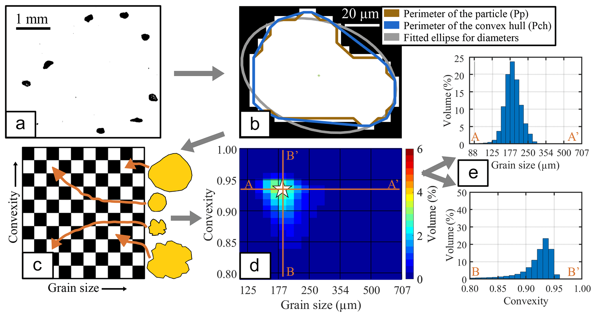
Figure 2(a) Binary image of sediment grains. (b) Computation of particle characteristics (note inversed black–white scale). (c) Assignment of grains to size–shape classes. (d) Grain size–shape distribution (ConD2d in the example; star marker designates the mode of the distribution). (e) Grain size (upper panel) and grain shape (lower panel) cross sections through the SSD along respectively A–A' and B–B'.
Table 2Summary of particle size and shape variables. The table shows lower and upper limits for the variables as well as the size of the respective size or shape classes. The range of interest designates the range over which the sediments studied here contain significant volume for a given variable. The φ unit refers to Krumbein's log base 2 grain size scale (Krumbein, 1938). The following letters were used in the equations for the size–shape variables: Pp (perimeter, or length along the particle boundary), Pch (convex hull or length along the convex points on the particle boundary), A (particle area), DB (minor diameter of ellipse fitted to particle), and DA (corresponding minor diameter).
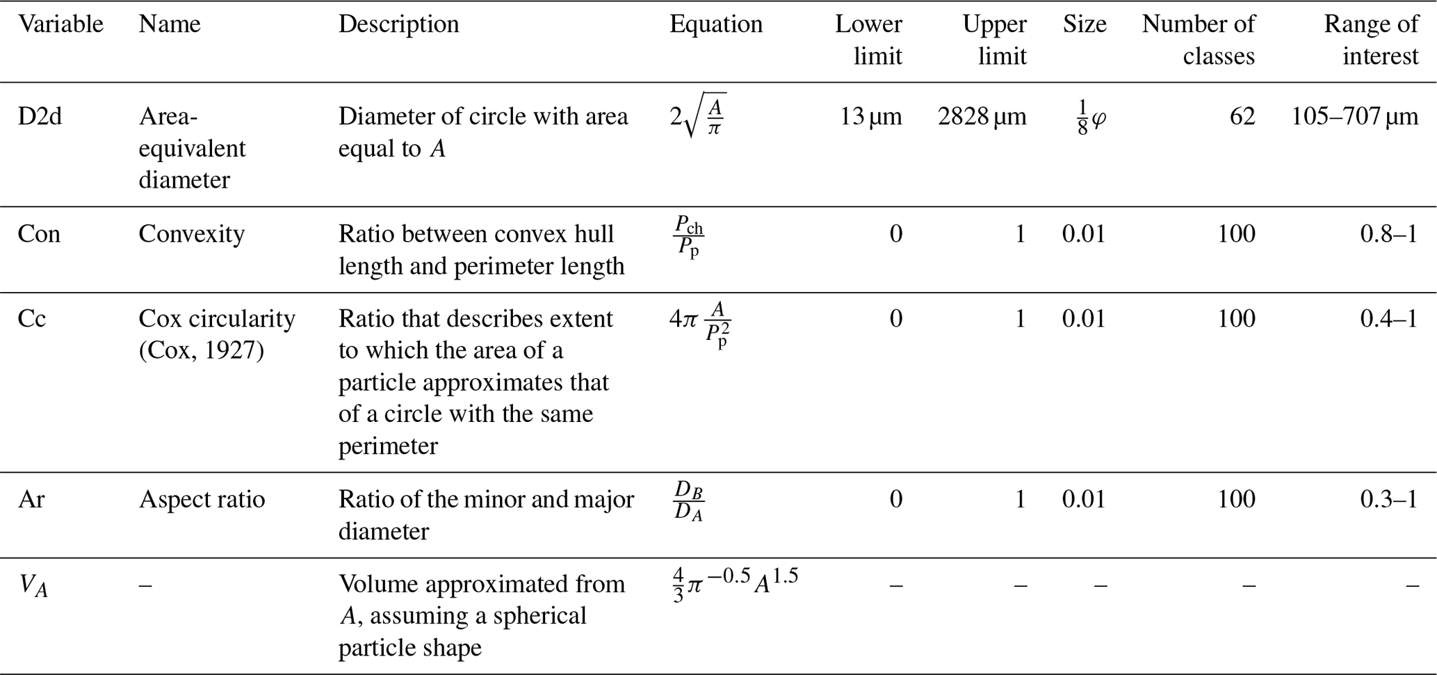
Image processing is carried out using a MATLAB script written by the first author, for which Fig. A2 shows a workflow diagram. The particle size and shape characteristics that form the output of this script are described in Table 2, and an example is given in Fig. 2b. In the first step of the script some limitations and conditions are set. Subsequently, the script iterates over each video, over each frame in the video, and over each particle found in the frames. For each particle, the length of its outer edge (perimeter) is computed as well as its area and the length of its convex hull (a polygon drawn around the particle without taking into account the concave areas). These basic parameters are stored for each particle. Particle size, volume, aspect ratio, convexity, and Cox circularity are subsequently computed from these basic parameters. It is important to note that the major and minor grain diameters, which are used to compute the aspect ratio, are based on the diameters of a fitted ellipse. These diameters are less sensitive to small-scale particle roughness than the traditional Feret diameters (Feret, 1930). “The” grain size of the particle is given in the form of an area-equivalent diameter (D2d; Table 2), essentially the average particle diameter of the two-dimensional image of the grain. Because the two-dimensional shape of the particle is known, grain size obtained by image analysis is more robust than traditional size measurements (e.g. sieving, laser diffraction, and settling) where an assumption has to be made of particle shape before computing size (Konert and Vandenberghe, 1997). We use ranges of interest in the graphs of size and shape distributions to focus on those size and shape classes that contain significant amounts of volume for the given dataset (Table 2).
2.3 Construction and unmixing of size–shape distributions
We explore the applicability of three shape parameters that are known to affect particle transport behaviour: convexity, Cox circularity (Cox, 1927), and aspect ratio (Table 2; Beal and Shepard, 1956; Dietrich, 1982; MacCarthy and Huddle, 1938; Winkelmolen, 1971; Shang et al., 2018). These parameters relate to different aspects of a particle's shape: aspect ratio describes the overall shape of a particle. In contrast, convexity is primarily affected by a particle's surface irregularity, whereas Cox circularity is affected by both.
Grain size–shape distributions (SSDs) are constructed from grain size (D2d; Table 2) and the three shape variables, resulting in the distributions named ArD2d, ConD2d, and CcD2d. The SSDs are created by assigning individual particles to their respective size–shape classes (Fig. 2c; Table 2). Next, the volume of the grains in each size–shape class is summed, and the distribution is normalised to a sum of 100 % using the total volume. This procedure gives rise to three-dimensional distributions (X is size, Y is shape, Z is volume) (Fig. 2d) that can be visualised as a combination of a grain size (X–Z) and a grain shape (Y-Z) distribution (Fig. 2e).
The endmember modelling algorithm AnalySize (Paterson and Heslop, 2015) is used to unmix the SSD datasets because it produces the most accurate results of the algorithms currently available (Van Hateren et al., 2017). The computed endmembers are hereafter referred to as endmember EMx−y, where x denotes the endmember number from coarse to fine and y denotes the total number of endmembers in the given endmember modelling solution. For example, the coarsest EM (endmember) of a dataset with four EMs is referred to as EM1−4.
The fit of endmember modelling solutions to the data is used to infer the most likely number of endmembers. The fit is described by variance squared, also termed the coefficient of determination (R2). We define two types of R2: (1) class-wise R2, denoting the fit per grain size class (grain–size distributions) or grain size–shape class (SSDs), and (2) sample-wise R2, denoting the fit per sample (Van Hateren et al., 2017). By increasing the number of endmembers, R2 will increase. However, at a certain point the increase in fit is not due to geologically significant endmembers but due to fitting of noise. We therefore seek the minimum number of endmembers sufficient to explain most of the variation in the dataset. In grain size data analysis, this minimum number of endmembers is traditionally estimated by a flattening off of the curve of average R2 versus the number of endmembers, also known as the inflection point (Prins and Weltje, 1999b; Weltje, 1997). However, tests with artificial grain size data have pointed out that this method sometimes yields an incorrect number of endmembers (Van Hateren et al., 2017). Rather than taking the average, we therefore use the full distribution of class-wise R2 to obtain more detailed information on the most likely number of endmembers (Prins and Weltje, 1999b; Van Hateren et al., 2017). In addition, we use the distribution of sample-wise R2.
2.4 Artificial datasets for testing and validation of the method
Artificial datasets with known endmembers and endmember abundances (Van Hateren, 2019) are used to evaluate (1) the accuracy of unmixing of SSDs under different mixing scenarios and (2) the potential of, and difference between, class-wise and sample-wise R2 for identification of the most likely number of endmembers in a SSD dataset. The known endmembers of the artificial datasets are hereafter referred to as input endmembers IEMx−y, similar to the notation for modelled endmembers.
Following an approach similar to Van Hateren et al. (2017), three datasets are created with increasingly complex mixing scenarios: the least complex dataset, 3EM_nonoise, is created using, as IEMs (input endmembers), three samples of the aeolian dune dataset with markedly different size–shape distributions (Fig. A3). Two-hundred sets of three random numbers are generated with a uniform distribution between 0 and 1 using a random-number generator. Each set of three numbers is subsequently normalised to sum to 1. The 200 sets represent the contributions of the IEMs to each artificial sample (endmember abundances). By multiplying each set of three random numbers with the three IEM SSDs, 200 artificial samples are generated.
The second dataset, 4EM_noise, is used to test accuracy of the method in the presence of noise and an additional endmember. Addition of noise decreases accuracy of unmixing results in grain size distribution datasets (Van Hateren et al., 2017). The IEMs of the 4EM_noise dataset are the same as those of the 3EM_nonoise dataset except for an additional endmember that, in terms of its grain size, is between the coarsest and intermediate IEM of the 3EM_nonoise dataset (Fig. A4). Noise is included in the dataset by multiplying the volume in each size–shape class of the artificial samples by a random number with a normal distribution characterised by a mean of 1 and a standard deviation of 0.05.
The third and most complex dataset, 4EM_noise_highmix, is similar to 4EM_noise (Fig. A5) but has different endmember abundances. This dataset is used to test the accuracy of the output for highly mixed datasets. In such datasets, one or more of the primary components do not form a dominant contribution to any of the samples. Highly mixed data significantly deteriorate accuracy of unmixing (Heslop, 2015; Van Hateren et al., 2017). We use the following mixing scenario: IEM1−4 occurs in only five samples at abundances between 0.2 and 1 (20 % and 100 %). IEM2−4, the highly mixed endmember, occurs in 100 samples at low abundance between 0.05 and 0.2 (5 % and 20 %). IEM3−4 and IEM4−4 occur in all 200 samples at randomly varying abundance.
Because the number of endmembers, the endmember abundances, and the endmember SSDs are known, the precision of the unmixing procedure can be determined from (1) the correlation between IEM SSDs and modelled endmember SSDs, (2) the correlation between the input and modelled endmember abundances, and (3) the correlation between the input and modelled data expressed as class-wise and sample-wise R2. Furthermore, the applicability can be assessed of class-wise and sample-wise R2 for identification of the most likely number of endmembers, which is an unknown in real-world datasets.
3.1 Endmember modelling results for the artificial datasets
3.1.1 Endmember modelling results for the 3EM_ nonoise dataset
Due to absence of noise in the 3EM_nonoise dataset, explained variance of the endmember modelling outcome reaches 100 % at three endmembers. Because model fit cannot be improved further, the AnalySize algorithm aborts at three endmembers (the algorithm fits a maximum of 10 endmembers for real-world datasets that naturally include noise). Figure 3 therefore displays class-wise R2 distributions for results with one to three endmembers (1EM to 3EM solutions). The “average” SSD of the dataset as well as the modelled endmembers are shown as contours to indicate the relevant size–shape classes. The 1EM solution fits the input data poorly, while the 2EM output increases model fit significantly but lacks explanatory power in the size–shape region that coincides with the missing third endmember (Figs. 3, A3). Using three endmembers increases goodness of fit of all size–shape classes to an R2 of 1. Figure A6a shows median sample-wise and class-wise R2 versus the number of endmembers. Class-wise R2 shows a near-linear increase from one to three endmembers, whereas the curve of sample-wise R2 inflects at two endmembers. In other words, the improvement in sample-wise R2 is significantly higher from one to two endmembers than it is from two to three endmembers.
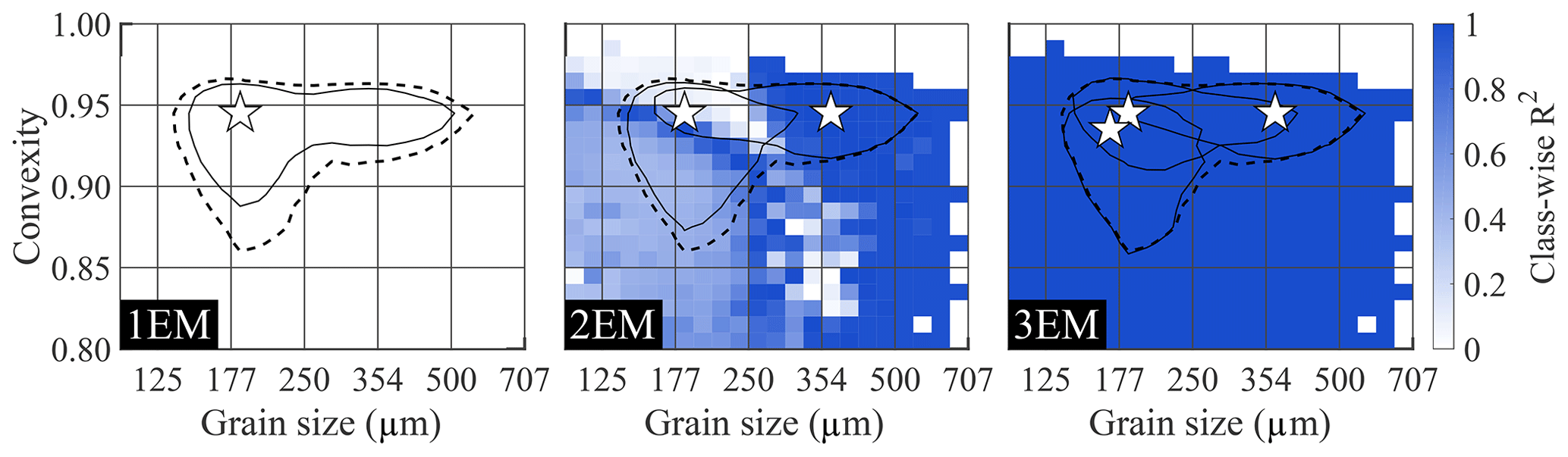
Figure 3Class-wise R2 distributions for endmember modelling results of the ConD2d 3EM_nonoise dataset from a 1EM up to a 3EM solution. Solid black lines denote endmember contours: lines drawn along those size–shape classes where the volume of the endmember SSD equals 0.5 %. The median SSD of the dataset (average SSD) is represented by a dashed line at 0.2 % volume. White stars denote the modes of the endmember size–shape distributions.
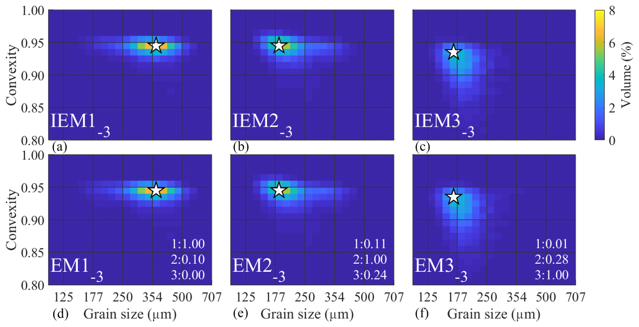
Figure 4Input endmembers (a–c) and determined endmembers (d–f) for the ConD2d 3EM_nonoise dataset, with R2 values denoting the fit between them (lower right corners). The first R2 value indicates the correlation of the determined endmember with IEM1−3, the second with IEM2−3, etc. White stars mark the modes of the SSDs.
Since the 3EM_nonoise dataset is noise-free and consists of three IEMs, an accurate 3EM solution should be identical to the input data, which is nearly the case (Fig. 4). The abundances show 100 % explained variance; however, linear trends between the original and determined abundances reveal a slope slightly higher than 1, meaning that high input abundances are calculated too high and that low input abundances are calculated too low (below input abundances of approximately 3 %, determined abundances go to zero) (Fig. A7a). Thus, the computed endmembers are, to a minor degree, still mixtures of the IEMs.
3.1.2 Endmember modelling results for the 4EM_noise dataset
Figure 5 shows class-wise R2 distributions of solutions for the 4EM_noise dataset. Similar to results for the 3EM_nonoise dataset, a 1EM solution fits the data poorly and a 2EM solution increases the fit significantly but lacks explanatory power in the intermediate and coarse size–shape regions. A 3EM solution fits the intermediate region significantly better but still lacks explanatory power in the coarse region. Compared to that of the 3EM solution, the class-wise R2 distribution of the 4EM solution displays an increase in R2 in the coarse range because EM1−4 more closely resembles IEM1−4 than EM1−3 resembles IEM1−4 (Figs. 5, A4). The increase in median class-wise R2 is small because the improvement occurs in relatively few size–shape classes (Fig. A6b, c). Median sample-wise R2 similarly increases by a low amount. The increase in sample-wise R2 diminishes from four endmembers onwards (Fig. A6c). Class-wise R2 even displays a minor decrease in fit. In contrast to results for the 3EM_nonoise dataset, the explained variance does not reach 100 %.
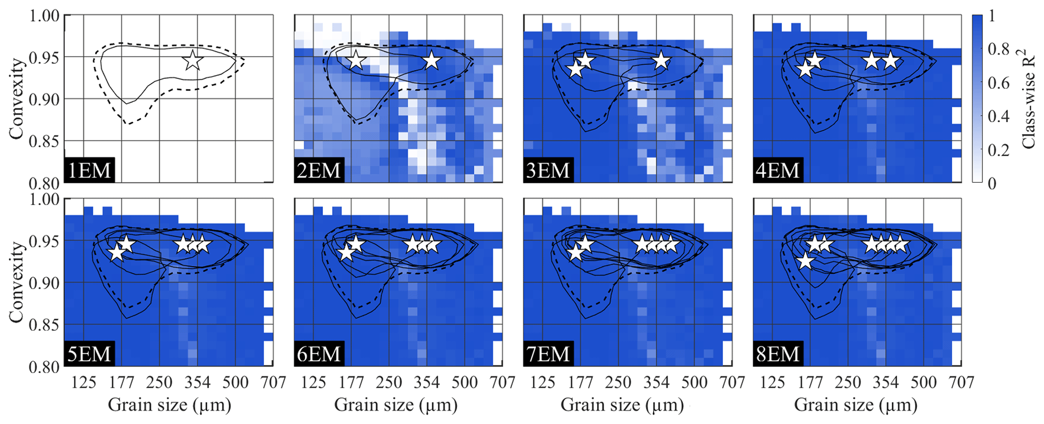
Figure 5Class-wise R2 distributions for endmember modelling results of the ConD2d 4EM_noise dataset. Solutions up to eight endmembers are shown. Solid black lines denote endmember contours: lines drawn along those size–shape classes where the volume of the endmember SSD equals 0.5 %. The median SSD of the dataset (average SSD) is represented by a dashed line at 0.2 % volume. White stars denote the modes of the endmember size–shape distributions.
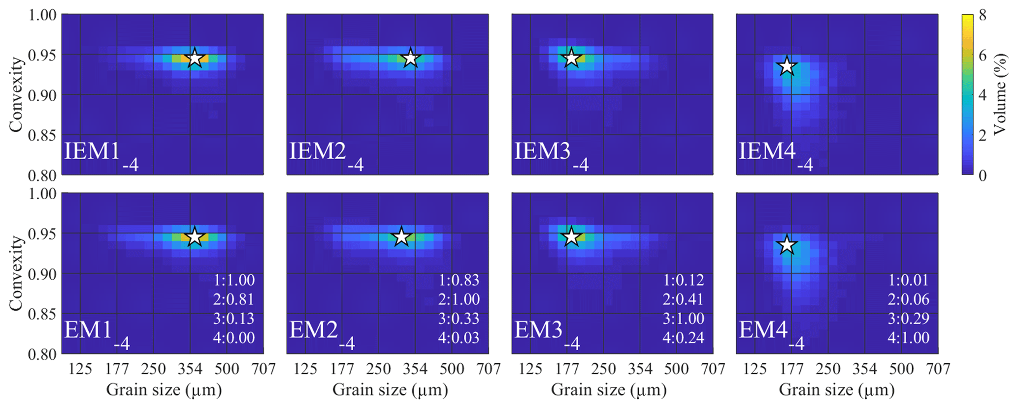
Figure 6Endmembers determined for the ConD2d 4EM_noise dataset. Input endmembers (top) are compared to determined endmembers (bottom) including R2 values. The first R2 value indicates the correlation of the endmember with IEM1−4, the second with IEM2−4, etc. White stars mark the modes of the SSDs.
Figure 6 compares the input and determined endmember SSDs. In spite of the noise added to this dataset, the determined endmembers are very similar to the IEMs. Calculated abundances fit the input abundances well, although minor scattering is present (Fig. A7b). Similar to the results for the noise-free dataset, linear trends have a slope higher than 1, indicating that the determined endmembers are, to a minor extent, mixtures of the IEMs.
3.1.3 Endmember modelling results for the 4EM_noise_ highmix dataset
Similar to the results in Sect. 3.1.1 and 3.1.2, the 1EM solution modelled for the 4EM_noise_highmix dataset fits the dataset poorly (Fig. 7). The 2EM class-wise R2 distribution is notably different from that of the 4EM_noise dataset: the entire coarse range (>350 µm) is not well reproduced. The reason for this disparity is that IEM1−4 and IEM2−4 are not represented in this solution, and thus the coarse range is underrepresented (Figs. A5, 7).
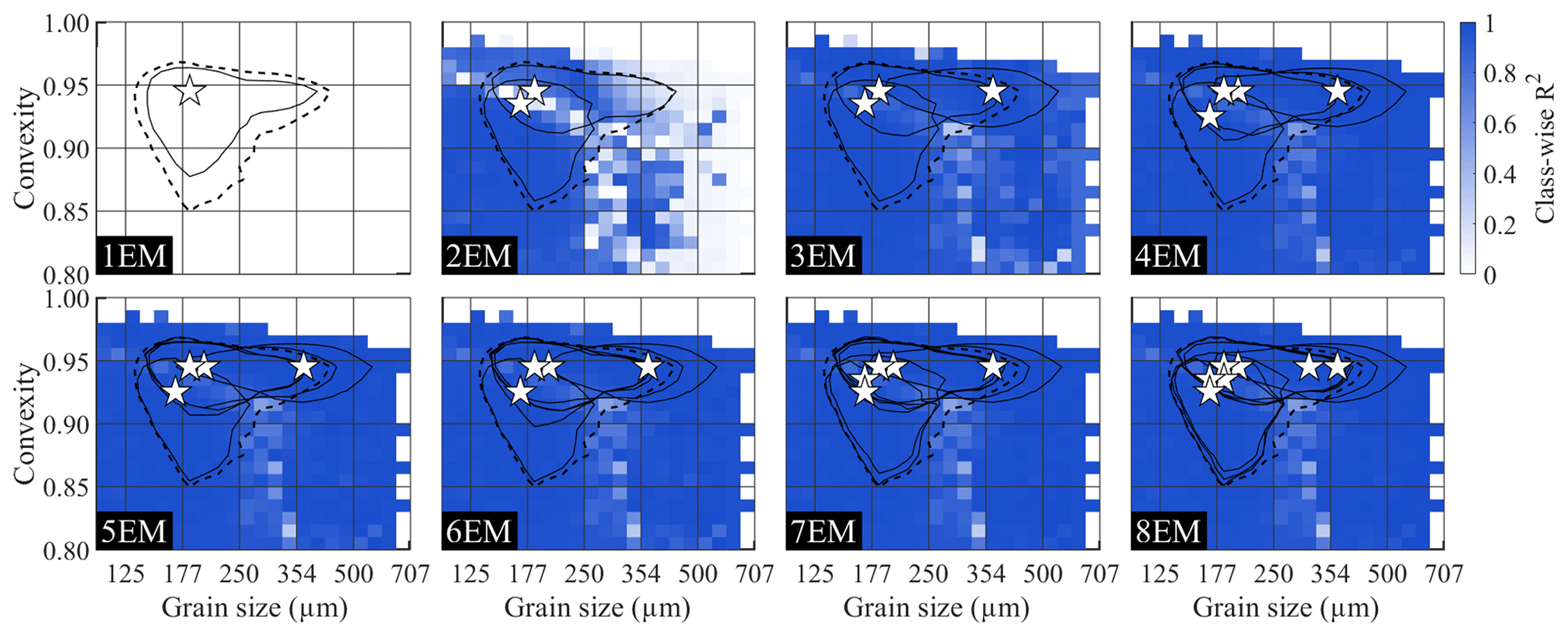
Figure 7Class-wise R2 distributions for endmember modelling results of the ConD2d 4EM_noise_highmix dataset. All solutions up to eight endmembers are shown. Solid black lines denote endmember contours: lines drawn along those size–shape classes where the volume of the endmember SSD equals 0.5 %. The median SSD of the dataset (average SSD) is represented by a dashed line at 0.2 % volume. White stars denote the modes of the endmember size–shape distributions.
A 3EM solution covers the coarser range, invoking a strong increase in class-wise R2 to a level comparable to that of the 4EM solution of the 4EM_noise dataset (Fig. 6d, e). In contrast to the results for the 4EM_noise dataset, addition of a fourth endmember does not result in a significant improvement of class-wise and sample-wise R2.
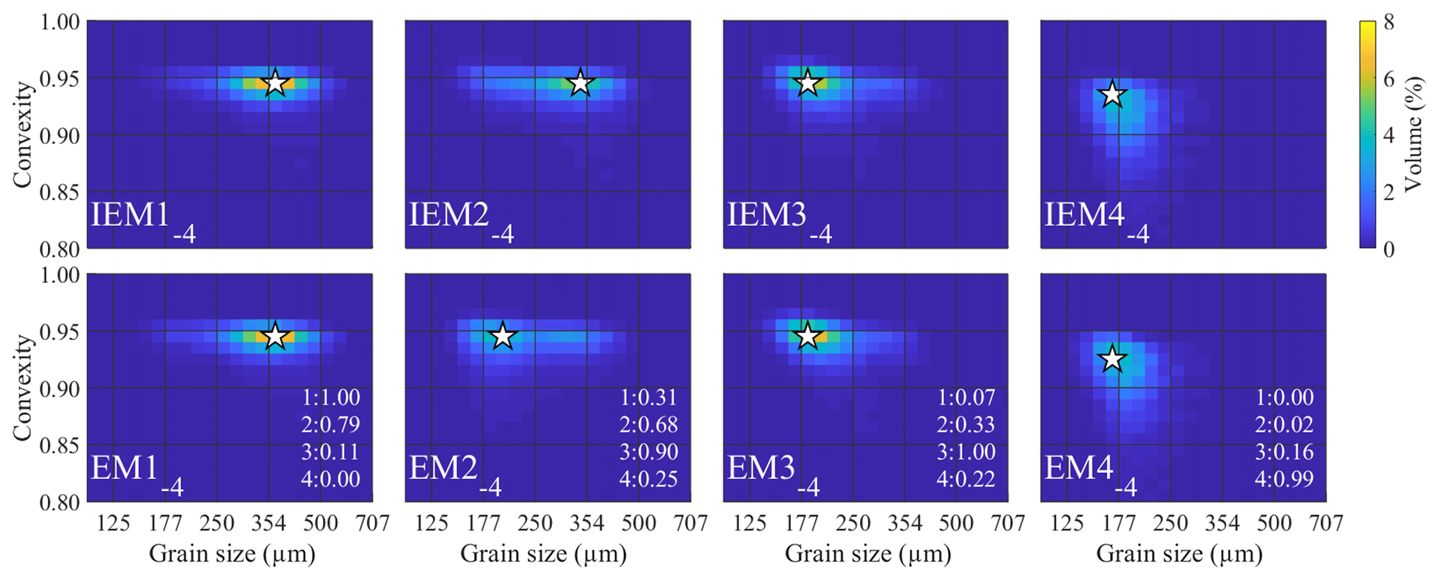
Figure 8Endmembers determined for the ConD2d 4EM_noise_ highmix dataset. Input endmembers (top) are compared to determined endmembers (bottom) including R2 values. The first R2 value indicates the correlation of the determined endmember with IEM1−4, the second with IEM2−4, etc. White stars mark the modes of the SSDs.
Size–shape distributions of the endmembers and IEMs are shown in Fig. 8. The 4EM solution computed for the 4EM_noise_highmix dataset differs in one notable aspect from that calculated for the 4EM_noise dataset: IEM2−4 is not identified as a primary component of the dataset. Rather, the SSD of EM2−4 more closely resembles IEM3−4, leading to overestimated abundances of EM2−4 and underestimated abundances of EM3−4 in the 4EM solution (Fig. A7c). However, the SSDs and the relative abundances of the 3EM solution show a good fit to the SSDs and abundances of the three non-highly mixed IEMs (Figs. A5, 7d).
3.2 Results for the aeolian dune dataset
Endmember modelling results for the aeolian dune dataset are presented in three subsections: statistics for the ConD2d dataset are shown first to derive the number of endmembers necessary to explain grain size–shape variability occurring in the aeolian deposits. Endmember SSDs and abundances of the robust solution are presented in the second subsection. The third subsection compares results of unmixing based on SSDs to results of unmixing based on grain size distributions (D2d).
3.2.1 Unmixing of the size–shape distributions
The trend of median class-wise and sample-wise R2 against the number of endmembers can be used as a primary indication of the number of primary components necessary for a good representation of the aeolian dune dataset. Class-wise R2 reaches a plateau at three endmembers, whereas sample-wise R2 inflects gradually between two and four endmembers (Fig. A8). This gives a first indication that the likely number of endmembers is between two and four.
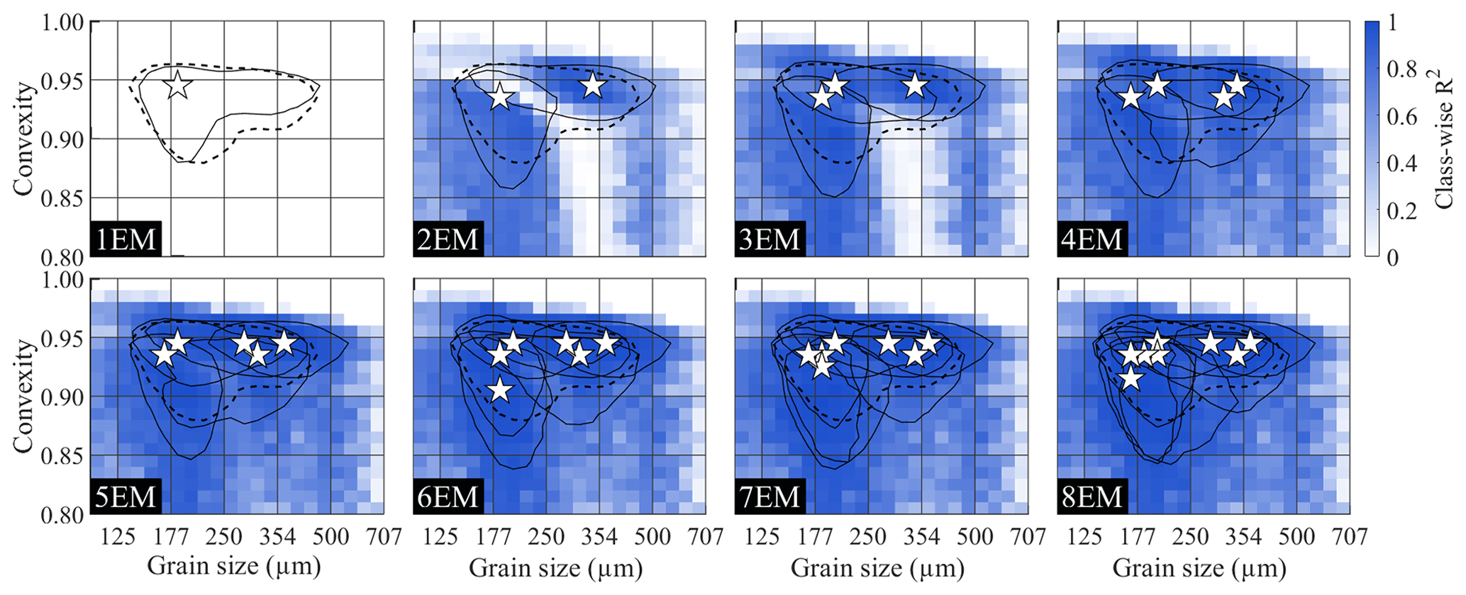
Figure 9Class-wise R2 for endmember modelling results of the ConD2d distributions of the aeolian dune dataset. All solutions up to eight endmembers are shown. Solid black lines denote endmember contours: lines drawn along those size–shape classes where the volume of the endmember SSD equals 0.5 %. The median SSD of the dataset (average SSD) is represented by a dashed line at 0.2 % volume. White stars denote the modes of the endmember size–shape distributions.
Two methods are employed to visualise the fit of the endmember solutions to the dataset in more detail. Class-wise R2 distributions show the fit per size–shape class (Fig. 9). The spatial distribution of sample-wise R2 is shown by plotting it on top of an aerial photograph of the study area (Fig. A9a). The goodness of fit of the samples is compared to the subregions based on geomorphology as shown in Fig. 1c, shown in simplified form in Fig. A9a, and described in Sect. 2.1. If the unmixing result fits poorly to samples from a specific subregion, it is likely that an additional endmember is needed to explain the data in that region.
One endmember is insufficient to capture the size–shape variability in the dataset: the class-wise R2 distribution shows low values across all size–shape classes (Fig. 9). The 1EM solution does not fit well to the samples either, as expressed by low sample-wise R2 (Fig. A8). The spatial distribution of sample-wise R2 for the 2EM solution shows a good fit to the sediment-trap samples of the hinterland. However, the fit to samples of the notch and foredune ridge is poor. The 3EM solution greatly improves fit in these subregions (Fig. A9a). Regarding the class-wise R2 distribution, the 2EM solution performs poorly in the range where its EM1−2 and EM2−2 overlap, indicating that an additional endmember is required to fit these classes (Fig. 9). A 3EM solution represents this intermediate size–shape range much better. Furthermore, comparison of the class-wise R2 distribution to the median data contour shows that this unmixing result performs well in the entire size–shape range where significant volume is present in the data (Fig. 9).
Although the 3EM solution displays high and evenly spread sample-wise R2, there are two regions that stand out: first, slightly lower explained variance occurs at those inland samples that are positioned downwind of fossil dunes that had their vegetation cover removed (Figs. A9a, 1b and c). A 4EM solution does not improve explained variance of these samples significantly (Fig. A9a). Second, the 3EM solution displays low sample-wise R2 on the northern foredune sampling transect, in a small region near the crest (Fig. A9a). This is improved by component EM2−4 of the 4EM solution, which occurs specifically in this region (Fig. A11). The specific geographical location of the component indicates that it has some geological significance. Furthermore, it is also determined in the 5EM and 6EM solutions (Fig. A10) and therefore is a robust component. However, it is of minor importance in terms of geographical extent and in terms of the number of samples it represents. The class-wise R2 distribution of the 4EM solution shows amelioration of fit below a convexity of 0.9 and above a size of 250 µm, but volume in this range is insignificant (Fig. 9). Further increasing the number of endmembers does not increase model fit significantly except that the 6EM solution increases sample-wise R2 for the inland samples downwind of unvegetated dunes (Figs. A9a, 1b and c). In conclusion, a 3EM output appears most robust, and it reproduces the bulk of spatial variability in grain size and shape, although a four-endmember solution locally improves sample-wise R2.
3.2.2 Endmember composition and abundances of the three-endmember solution
The endmember SSDs of the 3EM solution computed for the ConD2d distribution dataset differ markedly from one another (Fig. 10): most volume of coarse-grained EM1−3 is contained between 250 and 500 µm. Its mode lies at a grain size of 339 µm and a convexity of 0.945. This convexity dominates over the entire size range. The intermediate EM2−3 is finer-grained, with most of the volume between 160 and 350 µm. Its mode is positioned at a size of 201 µm and a convexity of 0.945. In contrast to EM1−3, it shows a gradual decline in convexity with increasing size. Most volume of fine-grained EM3−3 lies between 150 and 250 µm. Its mode is located at a size of 185 µm and a convexity of 0.935. It shows a strong decrease in convexity with increasing size.
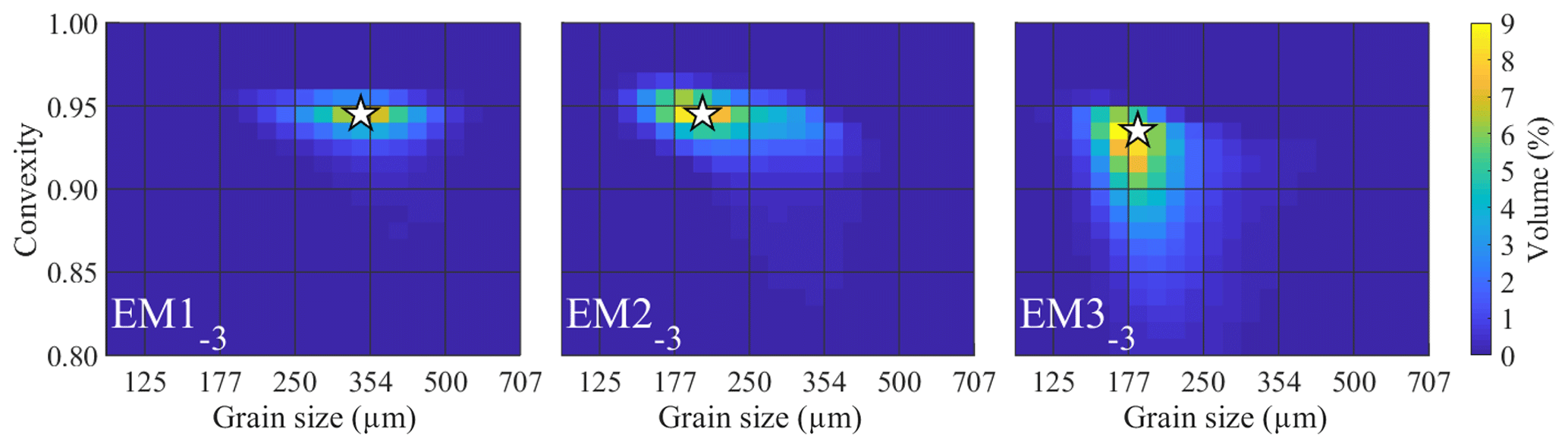
Figure 10SSDs of the ConD2d 3EM solution determined for the aeolian dune dataset. White stars mark the modes of the SSDs.
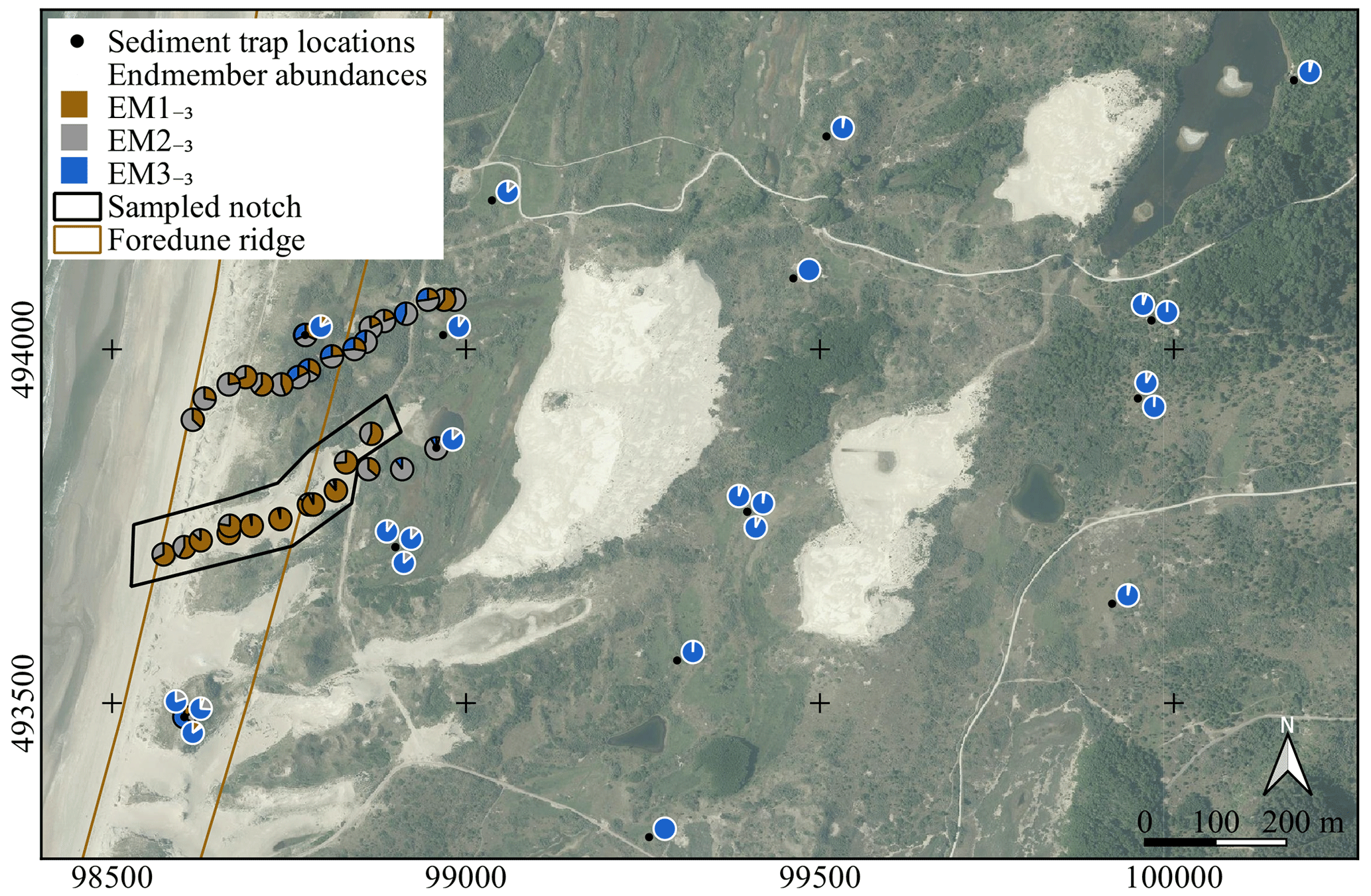
Figure 11Pie charts showing abundances of the 3EM solution computed for the ConD2d distributions of the aeolian dune dataset. Pie charts with a black outline denote surface samples and are plotted at the sampling location. Pie charts with a white outline denote sediment-trap samples and are plotted near the sampling location. The exact locations of sediment traps are marked by black dots. Two of the subregions defined in Fig. 1c are shown in simplified form. Aerial photograph © PDOK.nl, 2017.
The endmember abundances of the 3EM solution show a strong spatial differentiation that corresponds with morphological features: EM1−3 dominates the unvegetated notch that was dug through the foredune (average abundance 81 %). EM2−3 dominates most of the sparsely vegetated foredune (average abundance 46 %) as well as the vegetated area directly downwind of the sand lobe that progrades from the notch (average abundance 80 %). EM3−3 dominates the vegetated hinterland (trap rows B to D, average abundance 94 %) (Fig. 11). It is also noteworthy that samples from traps A1, A2, and B2 contain significantly more of EM3−3 than the surface samples taken at the same locations and thus also lower the average abundance of EM2−3 for the foredune (Figs. 11, 1b).
3.2.3 Comparison of results to traditional endmember modelling on grain size distributions
Besides the size–shape variable ConD2d, we also tested CcD2d and ArD2d. These variables make use of the shape variable Cox circularity and aspect ratio, respectively. In this section we intercompare endmember modelling results of the three size–shape variables. Furthermore, we compare the results using size–shape variables to results from traditional endmember modelling on grain size distributions (D2d). To enable direct comparison between grain size distributions and SSDs, the latter are transformed into grain size distributions by summation of the volumes of all shape classes per size class and subsequent renormalisation to 100 % (Fig. 12). The 3EM solution is used for the comparison. This number of endmembers is also robust for traditional grain-size-based endmember modelling: median R2 values level off at three endmembers (Fig. A12a), grain size classes with significant volume show high R2, indicating that class-to-class variability is well resolved (Fig. A12b), and sample-wise R2 is high throughout the fieldwork area, indicating that spatial variability is also well resolved (Fig. A9b).
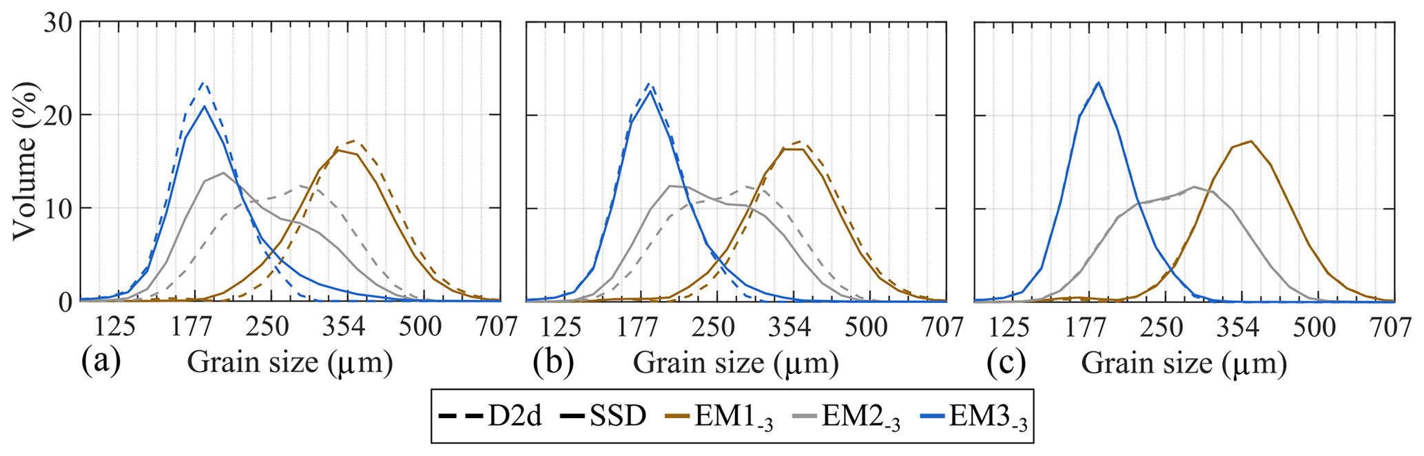
Figure 12ConD2d (a), CcD2d (b), and ArD2d (c) 3EM solutions determined for the aeolian dune dataset. The SSDs are displayed as grain size distributions (solid lines) and compared to grain size distributions of the D2d 3EM solution (dashed lines).
ConD2d endmember grain size distributions show significant deviations from those determined for D2d: most notably a finer modal size for EM2−3 but also a more extended fine tail for EM1−3 and coarse tail for EM3−3 (Fig. 12a). The grain size distributions of CcD2d show deviations at the same grain size ranges. However, the deviations are weaker than for ConD2d (Fig. 12b). In contrast, size distributions of the ArD2d endmembers equal those of D2d (Fig. 12c). Furthermore, the SSDs of ArD2d endmembers lack the trend in grain shape with grain size that was observed for ConD2d and CcD2d (Figs. 10, A13).
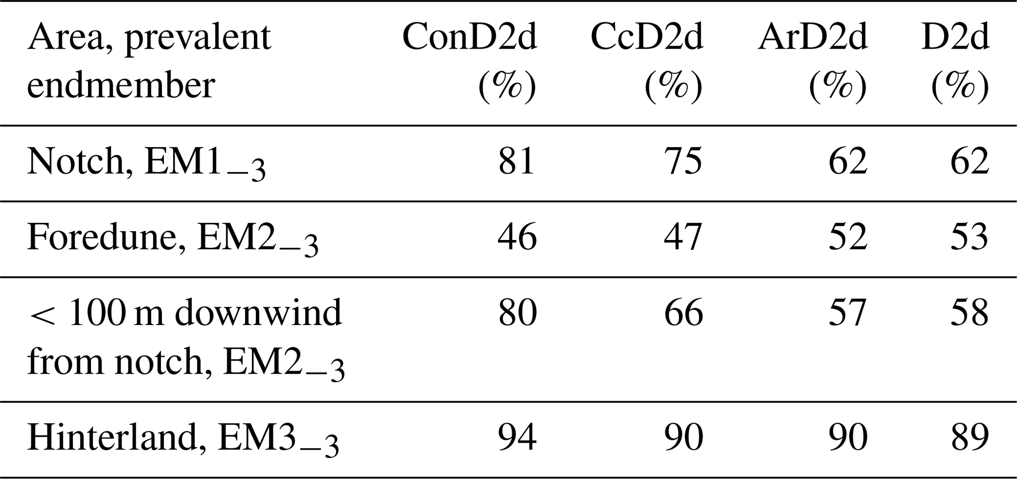
Table 3 and Fig. A14 compare endmember abundances for 3EM solutions of ConD2d, D2d, CcD2d, and ArD2d. The main trends of all variables correspond: EM1−3 prevails in the notch, EM2−3 on the foredune and in the vegetated area within 100 m downwind of the notch, and EM3−3 in the hinterland. However, differences exist between the variables: ConD2d and CcD2d show higher proportions of EM1−3 in the notch than ArD2d and D2d (Table 3). The four variables show similar proportions of EM2−3 on the foredune, but differences occur in the samples directly downwind of the notch. Here, proportions are highest for ConD2d, followed by CcD2d, D2d, and ArD2d (Table 3). Similarly, proportions of EM3−3 in the hinterland are slightly higher for ConD2d, followed by CcD2d, ArD2d, and D2d (Table 3). In summary, unmixing outcomes of ConD2d are generally most extreme, followed by CcD2d (they show the highest abundances of the dominant endmember). Results from ArD2d and D2d are generally less extreme. This clustering of results agrees with what was observed for the endmember grain size distributions in Fig. 12: ArD2d distributions are highly similar to those of D2d, whereas ConD2d and CcD2d distributions differ, respectively, strongly and weakly from the D2d distributions.
Table 3Average endmember abundances of the dominant endmember per subregion as defined in Fig. 1c.
4.1 Accuracy of endmember modelling on size–shape distributions
4.1.1 Accuracy of the unmixing methodology under different mixing scenarios
The precise 3EM solution for the 3EM_nonoise dataset confirms that the method is highly accurate under the condition that no noise is present in the dataset. Results for the 4EM_noise dataset indicate that computed endmembers remain correct reproductions of the input endmembers in the presence of noise. However, the noise induces minor deviations in the endmember proportions. Two conclusions can be drawn on the basis of the results for the 4EM_noise_highmix dataset. First, primary components that occur in a limited number of samples but at high proportions (IEM1−4) can be accurately determined by AnalySize. Second, highly mixed primary components (IEM2−4) cannot be determined accurately by AnalySize. This outcome is similar to results for highly mixed grain size distribution data (Van Hateren et al., 2017). The implication for real-world datasets is that highly mixed components will be overlooked during the endmember modelling procedure. However, our results indicate that the remaining endmembers and their relative proportions are computed accurately.
4.1.2 Methods for determination of the most likely number of endmembers
In the current study we use artificial datasets with a known number of endmembers. This allows us to test three methods for detection of the statistically feasible number of endmembers: median class-wise R2, median sample-wise R2, and class-wise R2 versus size and shape (a class-wise R2 distribution). The last is similar to a graph of class-wise R2 versus grain size for grain size data.
Our results for artificial datasets indicate that interpretation of the number of endmembers is straightforward in the absence of noise but ambiguous when noise is present: the noise-free dataset (3EM_nonoise) displays class and sample-wise R2 values of 1 when the number of determined endmembers equals the number of endmembers present in the dataset. In contrast, the R2 values for the noise-containing dataset (4EM_noise) never reach 1, which is more in line with endmember modelling results for real-world datasets. In this case, median R2 can only be used as a rough indication of the number of endmembers, since an “inflection point” (Prins and Weltje, 1999b; Weltje, 1997) is ill-defined: median R2 values for the dataset level off at three endmembers rather than four. A class-wise R2 distribution provides a better estimation of the number of endmembers: the presence of four endmembers is apparent from an increase in class-wise R2 in the coarser size range going from a 3EM to a 4EM solution. The presence of the highly mixed endmember in the dataset 4EM_noise_highmix is not apparent from the class-wise R2 distribution, indicating that such an endmember will likely be ignored in the endmember modelling of real-world data.
There are two additional conceivable methods for determination of the geologically feasible number of endmembers: (1) a graph of sample-wise R2 against depth (core or outcrop) or against sample location (spatial data such as the aeolian dune dataset) and (2) using samples of known origin to demonstrate the geological meaning of the endmembers (Weltje and Prins, 2003). These two methods cannot be tested with artificial data and thus will be discussed using the aeolian dune dataset.
Results for the aeolian dune dataset indicate that spatially resolved sample-wise R2 can be used to determine the number of endmembers, especially when the spatial distribution of model fit is compared to known geomorphology of the area. For example, the 2EM solution fits poorly to the samples of the notch and foredune area. This indicates that two primary components are insufficient to describe the aeolian processes occurring in these subregions. The 3EM solution satisfactorily fits all main subregions, indicating that it captures the main transport processes that are active in the study area. The aeolian dune dataset also provides two examples of modern-day samples of known transport processes that can be used as reference material for palaeo-studies. Surface samples from the notch area can be used as a reference for aeolian bedload sediment because the surface of the notch area was characterised by aeolian current ripples. Furthermore, samples from sediment traps, especially from rows C and D, which are furthest land-inward (Fig. 1b), can be used as a reference for aeolian suspension because (1) the distance from the main source areas (beach and notches) excludes modified saltation from reaching the traps, (2) land-inward from the foredune ridge, denser vegetation rules out new entrainment of sediment (Arens et al., 2002; Lancaster and Baas, 1998), and (3) the height of the sediment traps further reduces the chance of contamination by local saltation.
4.2 The value of endmember modelling on size–shape distributions: implications of the aeolian dune dataset
4.2.1 Geological significance of the three-endmember ConD2d model
The spatial distribution of endmembers of the 3EM solution relates strongly to the geomorphology of the area: EM1−3 occurs mainly on the bare surfaces of the beach and notch, EM2−3 occurs on the sparsely vegetated foredune and within the vegetated area directly downwind of the notch, and EM3−3 occurs in the vegetated hinterland. This geographical differentiation suggests that the endmembers are linked to the three aeolian processes known to operate on a beach to dune transect: (1) bedload, consisting of saltation, reptation, and creep, the motions of which are predominantly affected by gravity; (2) modified saltation, which is affected by both gravity and turbulence; and (3) suspension, of which the motions are predominantly affected by turbulence (Arens et al., 2002; Hunt and Nalpanis, 1985).
As mentioned in Sect. 4.1.2, aeolian current ripples on the supratidal beach and in the notch confirm that EM1−3 is linked to the bedload population. Component EM2−3 specifically occurs on the windward and leeward slope of the foredune. Several processes on the foredune increase the proportion of grains travelling in modified saltation (Arens et al., 2002). (1) On the windward slope of the foredune, relief and marram grass induce turbulence, thereby increasing the proportion of grains that travel in modified saltation and suspension. (2) At the same time, the vegetation partly impedes bedload transport. (3) At the foredune crest, flow separation induces even stronger vertical air motion, forcing the grains into short-term suspension. The grains that are less susceptible to turbulence are deposited at the leeward side of the foredune (modified saltation population), whereas the grains that are more susceptible to turbulence (the true suspension population) travel further land-inward, where EM3−3 dominates. As stated in Sect. 4.1.2, the interpretation of EM3−3 as a suspension component is further corroborated by the distance from the source (beach and notches), the dense vegetation in the hinterland, and the fact that the sediment traps are at approximately 1.5 m a.g.l. Sediment traps on the foredune also show a high contribution of EM3−3, which is on average higher than that of the surface samples at the same location. This is likely related to the height of the traps, causing them to trap the sediment that is in transport (suspended load and modified saltation) rather than the sediment that is deposited (bedload and modified saltation).
The three endmembers were also set apart by a markedly different shape of their size–shape distributions: the bedload population was characterised by a constant grain regularity with increasing size, the modified saltation population by a minor decrease in grain regularity, and the suspended population by a strong decrease in grain regularity. These differences are likely caused by differences in size–shape sorting between the aeolian transport modes. Movements of grains in saltation are driven mainly by gravity (Hunt and Nalpanis, 1985), which is a function of particle mass. Because the beach sediments in our fieldwork area are of uniform density with negligible heavy mineral content (Eisma, 1968), particle mass is mainly determined by particle size. Size, not shape, is therefore the predominant sorting agent during saltation. Eisma (1965) furthermore inferred that it is likely that surface creep favours spherical grains because they roll more easily. It therefore follows that the overall bedload population should show relatively regularly shaped grains and no significant trend of grain shape with grain size. This is indeed the case for EM1−3.
Settling of grains in suspension is driven by gravity and restrained by aerodynamic drag of a particle. The latter factor also depends on grain shape: irregular grains have more drag and thus settle slower (Komar and Reimers, 1978) and are also more susceptible to turbulence. It therefore makes sense that the SSD of suspension component EM3−3 shows a strong decrease in grain regularity with increasing size: the irregularity of the coarser grains compensates for their larger weight. Chinese loess deposits are on the order of 2–10 times finer-grained than EM3−3 and show a similar decrease in grain regularity with increasing size (Shang et al., 2018). This indicates that (1) a decrease in grain regularity with increasing size is characteristic of sediments transported in aeolian suspension, and (2) for a given transport mode and a similar grain shape range, the grain size of sediment depends on, and is a reflection of, transport conditions (amount of transport energy available and transport distance). SSDs are therefore a good indication of the mode of transport; grain size distributions are not.
Modified saltation is a process that is intermediate between saltation and suspension: grains are saltating (sorted by susceptibility to gravity) but are also shortly suspended (sorted by susceptibility to gravity and turbulence). The size–shape distribution of EM2−3 is indeed intermediate between EM1−3 and EM3−3, both in terms of its grain size and its minor decline in grain regularity with increasing grain size.
4.2.2 A comparison of traditional grain-size-based and novel size–shape-based endmember modelling
Endmember distributions obtained using size–shape variable ArD2d are remarkably similar to those obtained using traditional size-based endmember modelling (D2d). This suggests that grains are not sorted by their aspect ratio. However, Shang et al. (2018) did observe sorting of aspect ratio during aeolian transport. This incongruity may be explained by the difference in how aspect ratio was defined in the two studies: we defined aspect ratio based on the major and minor diameters of ellipses fitted to the particles. These diameters represent the overall particle shape, since their length is not sensitive to small-scale particle roughness: the ellipse fitting procedure “averages out” small humps. In contrast, the major and minor Feret diameters as used in Shang et al. (2018) are affected by such small humps.
In contrast to ArD2d, endmember modelling results of CcD2d and especially ConD2d differ from D2d (grain size): the mode of their intermediate endmember is significantly finer-grained, and it overlaps more substantially with EM3−3. This overlap may actually be the cause of the observed difference: endmember modelling on size–shape distributions would be more suitable for identification of an endmember that strongly overlaps with another in terms of grain size but differs in grain shape. Of the three studied size–shape variables, results of ConD2d show the strongest unmixing (highest abundances of the dominant endmember). This indicates that ConD2d may be the most appropriate variable for the identification of transport processes.
We introduce a novel method that can be used to reconstruct sediment transport processes from aeolian deposits. The method makes use of endmember modelling on grain size–shape distributions, which are constructed from grain size and shape data obtained by dynamic image analysis. Tests with artificial size–shape distribution datasets indicate that the known endmembers and endmember mixing proportions are accurately computed by the method, even when noise is present in the data. Endmembers with limited occurrence are also identified; highly mixed components, however, cannot be determined accurately. The tests also point out that the distribution of the fit of unmixing results per size–shape class (the class-wise R2 distribution) can be used to indicate the number of endmembers present.
The size–shape distribution unmixing method is also applied to real-world data from an active aeolian system in the Dutch coastal dunes. Results show that a comparison of the spatial distribution of model fit (sample-wise R2) to local geomorphology further increases insight into the number of endmembers present. The geological meaning of endmembers can be validated by comparing their size–shape distributions to reference samples of different transport processes.
Three endmembers are determined for the aeolian dune dataset. The spatial distribution of these endmembers is in accordance with the local geomorphology and reflects the three dominant aeolian transport processes known to occur along a beach to dune transect: bedload, modified saltation, and suspension. These processes are characterised by distinctly different endmember size–shape distributions, resulting from differential (size and) shape sorting: with increasing size, bedload shows a constant grain shape, modified saltation a minor decrease in grain regularity, and suspension a strong decrease in grain regularity (when using convexity or Cox circularity as shape parameter).
Compared to traditional endmember modelling on grain size distributions, unmixing of SSDs gives rise to different endmember grain size distributions due to shape sorting effects. Results of the new method also show higher proportions of the dominant endmembers, indicating a better discrimination of the aeolian transport processes (especially when using convexity as shape parameter). The principal advantage of the new method, however, is that the characteristic shapes of the endmember size–shape distributions can be used as a fingerprint of the transport mode. The new method therefore resolves the ambiguity that arises when the transport mode is reconstructed using grain size distributions.
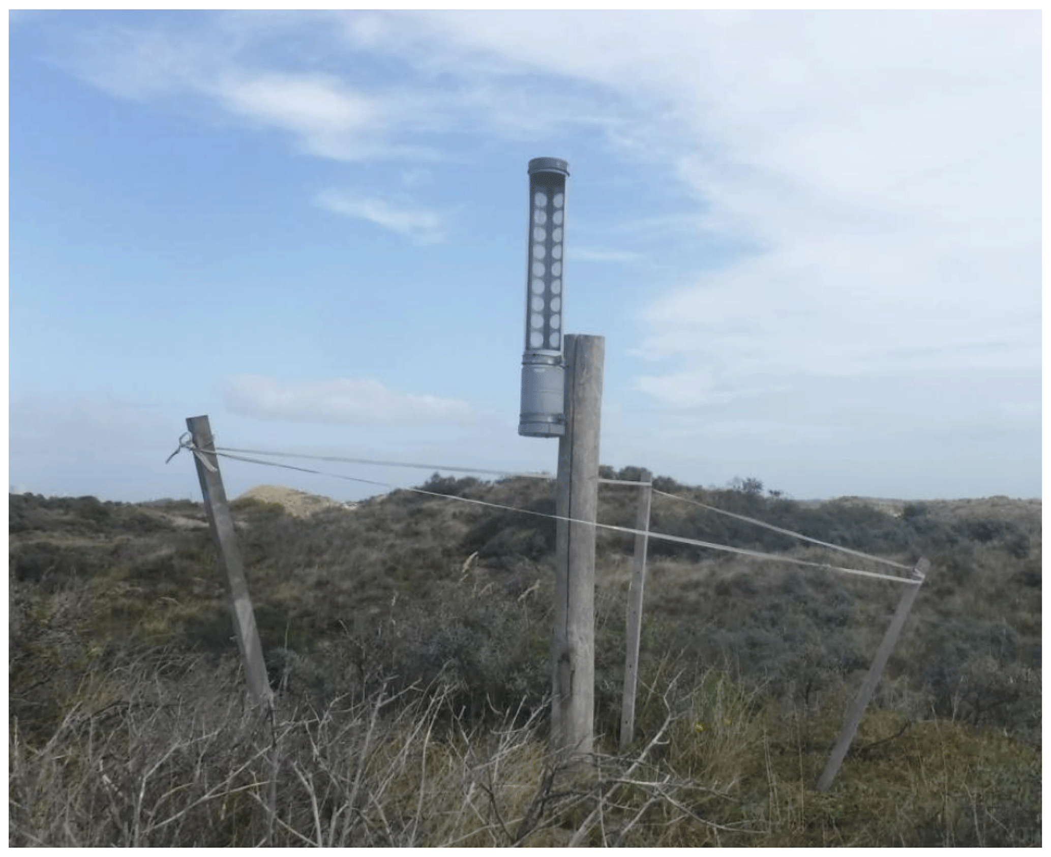
Figure A1Sediment trap on a vegetated dune.
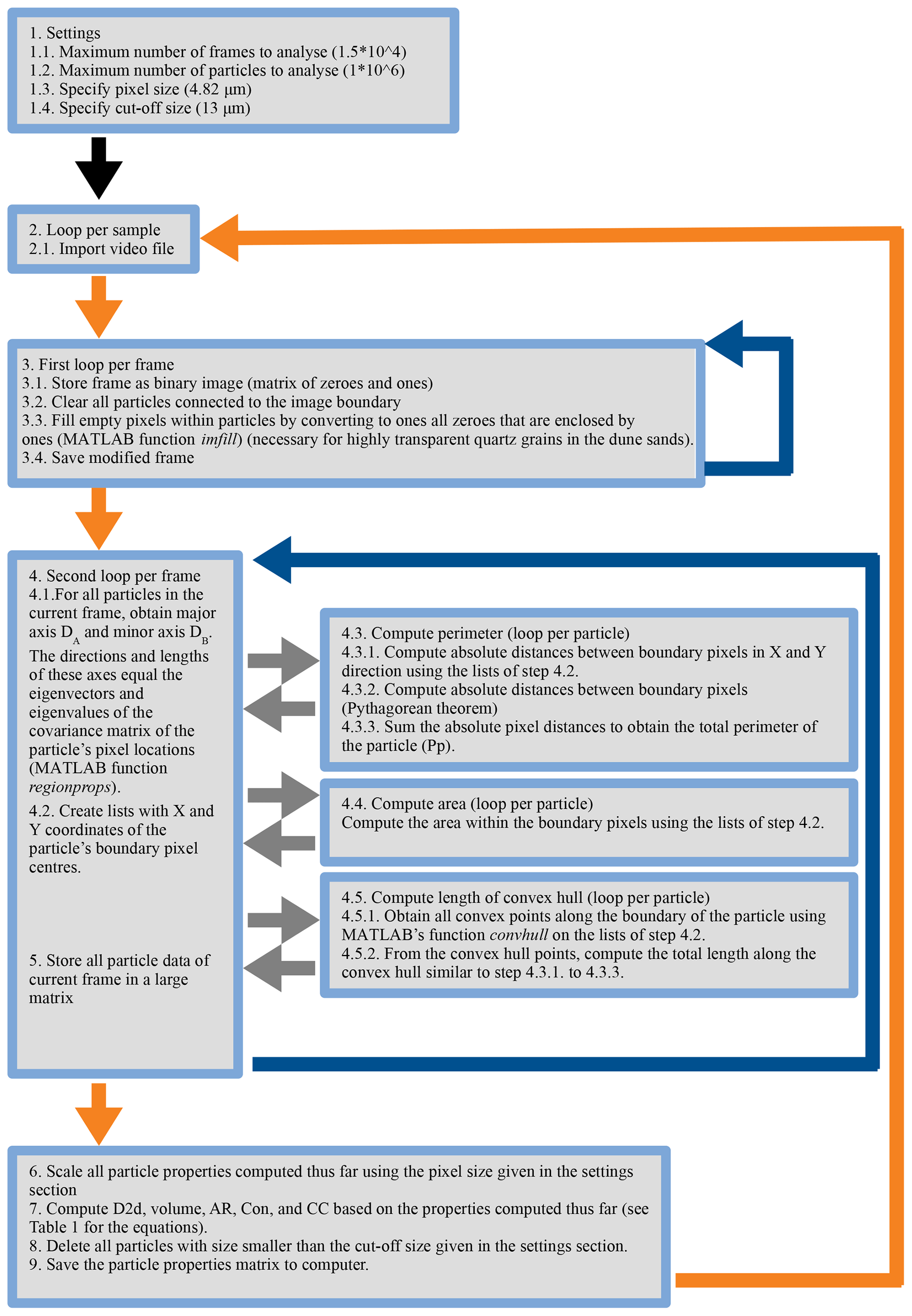
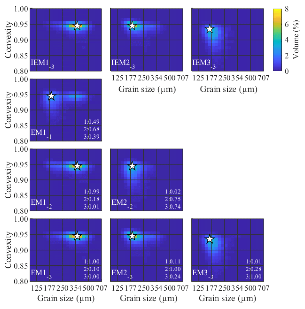
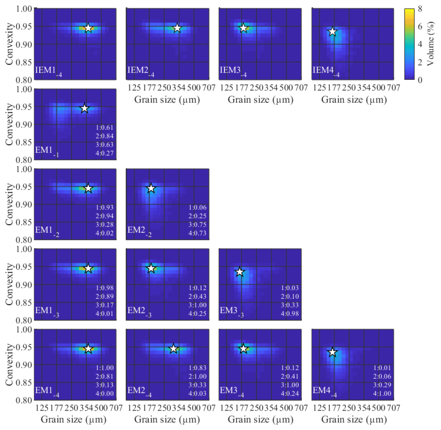

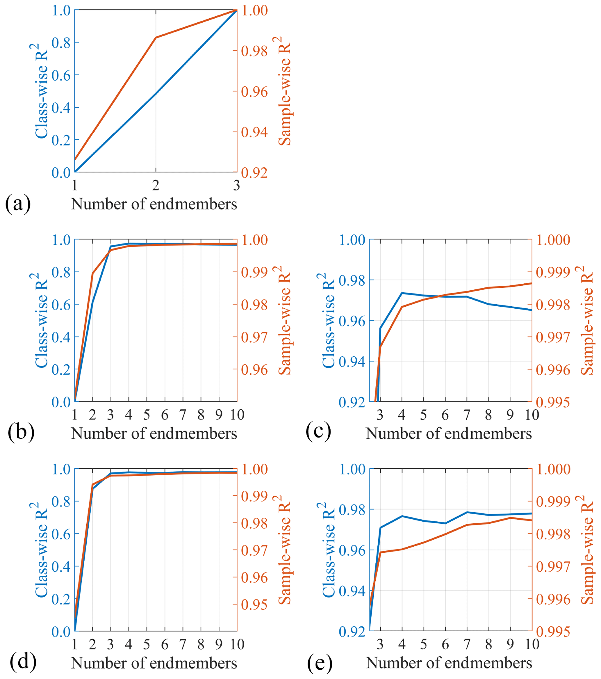
Figure A6Median class- and sample-wise R2 versus the number of endmembers for the artificial datasets: 3EM_nonoise (a), 4EM_noise (b, c), and 4EM_noise_highmix (d, e). Panels (c) and (e) zoom in on panels (b) and (d).
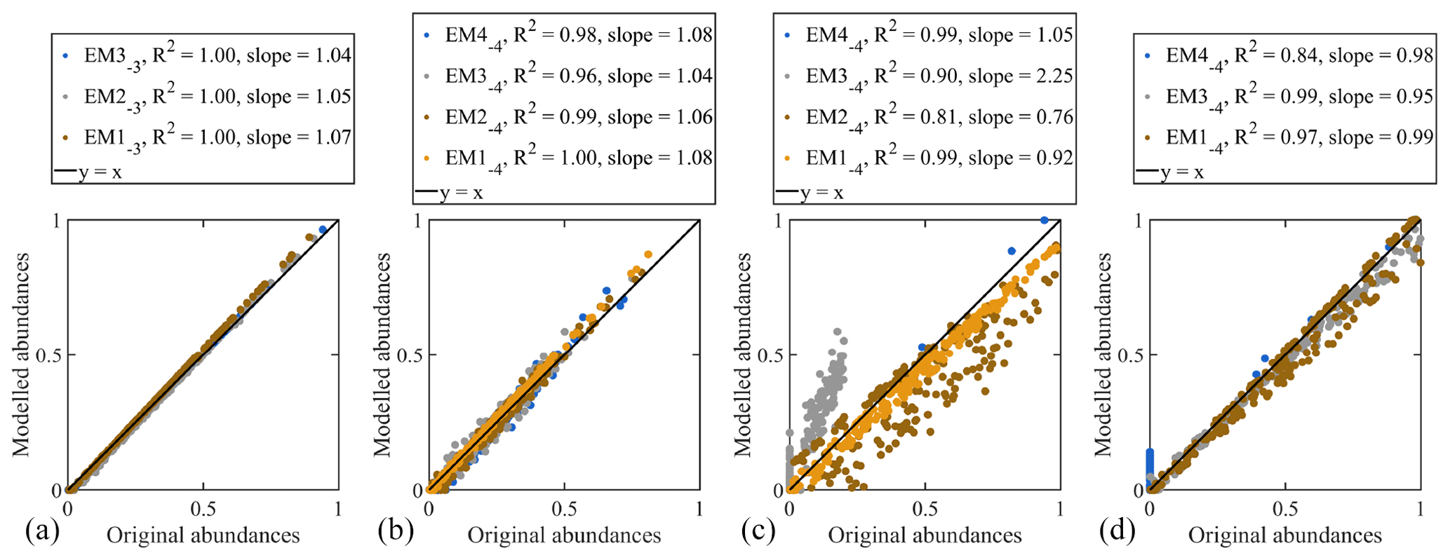
Figure A7A comparison of modelled and input endmember abundance for the artificial datasets (a: 3EM solution for 3EM_nonoise, b: 4EM solution for 4EM_noise, c: 4EM solution for 4EM_noise_highmix, d: 4EM solution for 4EM_noise_highmix, but without the highly mixed endmember).
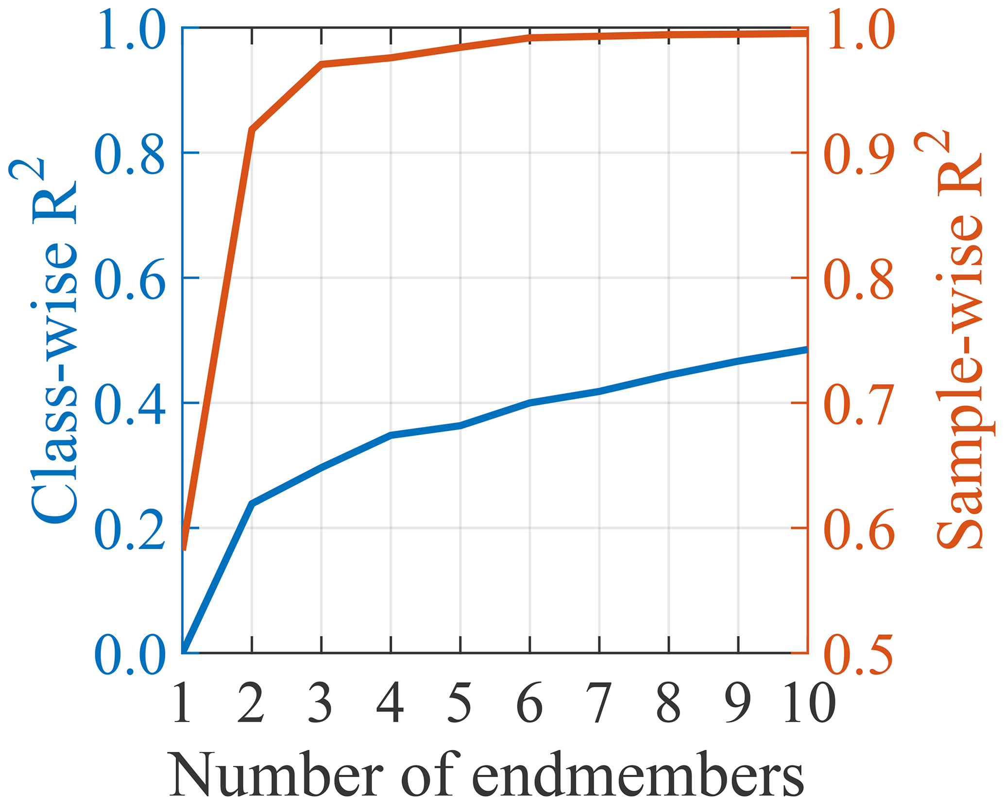
Figure A8Median class- and sample-wise R2 versus the number of endmembers for the ConD2d distribution dune dataset.

Figure A9Sample-wise R2 plotted over the sample locations for variable ConD2d (a) and variable D2d (b). The first interval of the colour scale is enlarged to elucidate the changes in R2, which mainly occur above a value of 0.9. Points with a black outline denote surface samples and are plotted at the sampling location. Points with a white outline denote sediment-trap samples and are plotted near the sampling location. The exact locations of sediment traps are marked by white dots. Two of the subregions defined in Fig. 1c are shown in simplified form. Aerial photograph © PDOK.nl, 2017.
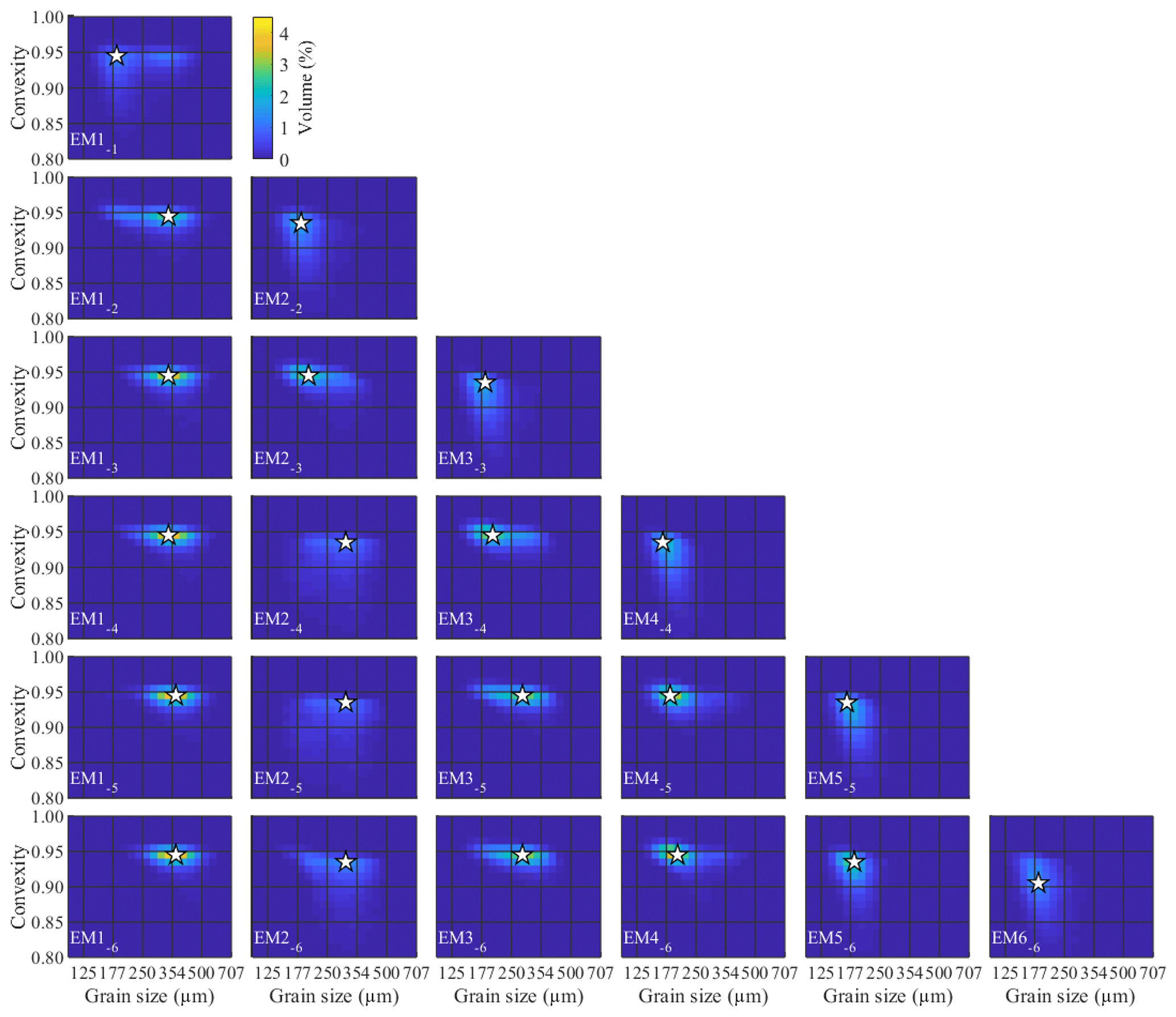
Figure A10Endmember distributions computed for the ConD2d dune dataset (1EM to 8EM solutions).
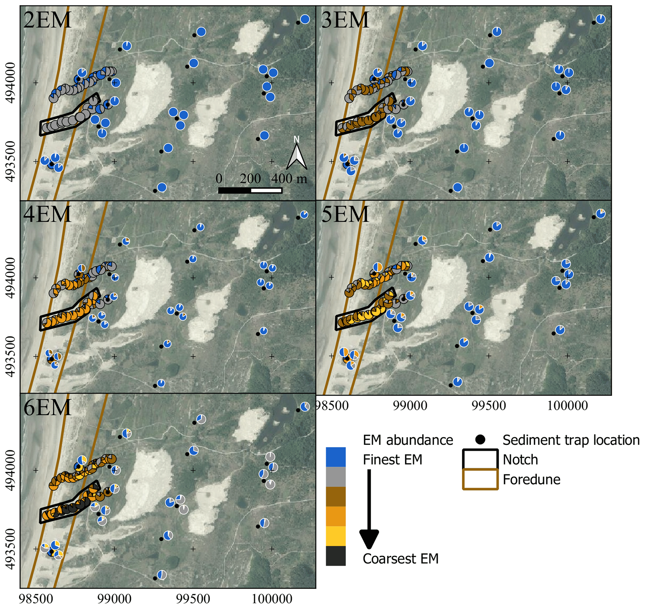
Figure A11Endmember abundances for variable ConD2d determined for the dune dataset. Pie charts with a black outline denote surface samples and are plotted at the sampling location. Pie charts with a white outline denote sediment-trap samples and are plotted near the sampling location. The exact locations of sediment traps are marked by black dots. Two of the subregions defined in Fig. 1c are shown in simplified form. Aerial photograph © PDOK.nl, 2017.
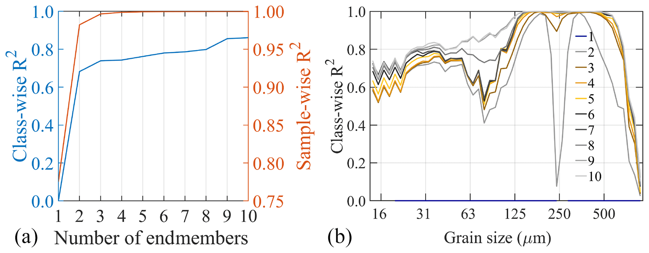
Figure A12Median class-wise and sample-wise R2 for D2d endmember modelling results of the dune dataset (a) and size-resolved class-wise R2 (b).
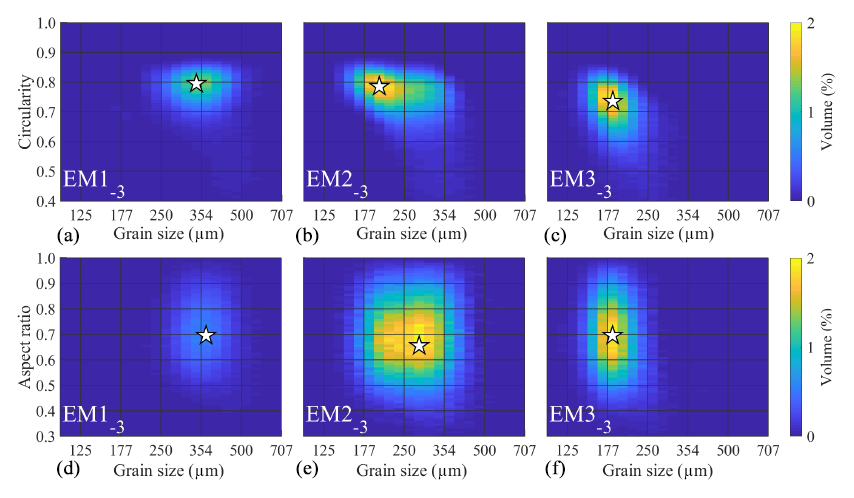
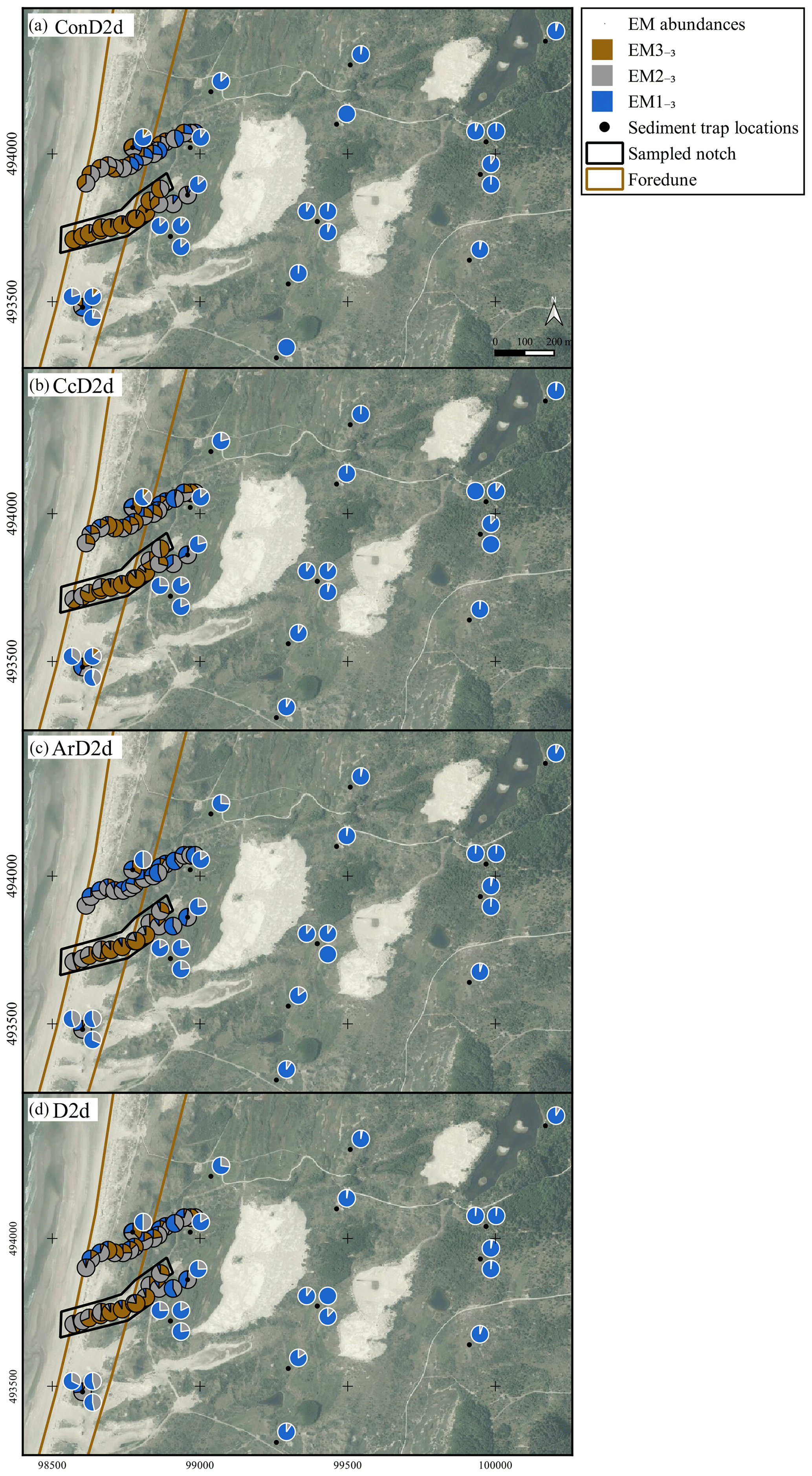
Figure A14Pie charts showing abundances of the 3EM solution determined for the ConD2d (a), CcD2d (b), ArD2d (c), and D2d (d) distributions of the dune dataset. Pie charts with a black outline denote surface samples and are plotted at the sampling location. Pie charts with a white outline denote sediment-trap samples and are plotted near the sampling location. The exact location of sediment traps is marked by black dots. Two of the subregions defined in Fig. 1c are shown in simplified form. Aerial photograph © PDOK.nl, 2017.
Data are available from the PANGAEA database (https://doi.org/10.1594/PANGAEA.909106; van Hateren, 2019).
JAvH wrote the initial draft of the paper; devised a way to integrate grain size and shape data; designed the code used for image processing, data processing, and data visualisation; and performed laboratory analyses. UvB performed fieldwork in the Nationaal Park Zuid-Kennemerland, laying the foundation for the dune dataset. He also performed laboratory analyses, performed initial tests on shape sorting during aeolian transportation, and helped improve the draft versions of the paper. SMA initiated and continued the sediment monitoring project in the Nationaal Park Zuid-Kennemerland using sediment traps. He also helped improve the initial draft of the paper. RTvB helped improve writing and construction of the paper and provided feedback on the method. MAP conceived the idea of endmember modelling of integrated size and shape data for a better understanding of sedimentological processes, performed fieldwork in the Nationaal Park Zuid-Kennemerland, initiated grain size and shape analysis on the dune sediments, helped improve the draft versions of the paper, and provided feedback and discussion on how to implement the method.
The authors declare that they have no conflict of interest.
We would like to thank Jeroen van der Lubbe (research associate in palaeoceanography and palaeoclimatology at Cardiff University and visiting fellow at the Vrije Universiteit Amsterdam) for his contributions to the image processing script and general discussion on image processing of sedimentary grains. We would furthermore like to thank Kay Beets (Vrije Universiteit Amsterdam) for his insights and his role in student projects in the Dutch coastal dunes. Martine Hagen (Vrije Universiteit Amsterdam) is thanked for general support during execution of the lab work. We would also like to express our gratitude to Marieke Kuipers and Hubert Kivit of the water company PWN for granting permission to perform the study in the Nationaal Park Zuid-Kennemerland, for their encouragement, and for their general support. Furthermore, we thank Gerard van Zijl (PWN) for maintenance of the sediment traps and collection of sediment-trap samples. Bachelor students Nick van der Veen, Paul Much, and Marenqo van der Noll are thanked for fieldwork and sample collection in the Nationaal Park Zuid-Kennemerland.
This paper was edited by Patricia Wiberg and reviewed by Simon Blott and one anonymous referee.
Arens, S. M., Van Boxel, J. H., and Abuodha, J. O. Z.: Changes in grain size of sand in transport over a foredune, Earth Surf. Proc. Land., 27, 1163–1175, https://doi.org/10.1002/esp.418, 2002.
Arens, S. M., Mulder, J. P., Slings, Q. L., Geelen, L. H., and Damsma, P.: Dynamic dune management, integrating objectives of nature development and coastal safety: examples from the Netherlands, Geomorphology, 199, 205–213, https://doi.org/10.1016/j.geomorph.2012.10.034, 2013.
Beal, M. A. and Shepard, F. P.: A use of roundness to determine depositional environments, J. Sediment. Res., 26, 49–60, https://doi.org/10.1306/74D704B6-2B21-11D7-8648000102C1865D, 1956.
Cox, E. P.: A method of assigning numerical and percentage values to the degree of roundness of sand grains, J. Paleontol., 1, 179–183, 1927.
Dietrich, W. E.: Settling velocity of natural particles, Water Resour. Res., 18, 1615–1626, https://doi.org/10.1029/WR018i006p01615, 1982.
Dietze, E., Hartmann, K., Diekmann, B., IJmker, J., Lehmkuhl, F., Opitz, S., Stauch, G., Wünnemann, B., and Borchers, A.: An end-member algorithm for deciphering modern detrital processes from lake sediments of Lake Donggi Cona, NE Tibetan Plateau, China, Sediment. Geol., 243, 169–180, https://doi.org/10.1016/j.sedgeo.2011.09.014, 2012.
Dietze, E., Maussion, F., Ahlborn, M., Diekmann, B., Hartmann, K., Henkel, K., Kasper, T., Lockot, G., Opitz, S., and Haberzettl, T.: Sediment transport processes across the Tibetan Plateau inferred from robust grain-size end members in lake sediments, Clim. Past, 10, 91–106, https://doi.org/10.5194/cp-10-91-2014, 2014.
Eisma, D.: Eolian sorting and roundness of beach and dune sands, Neth. J. Sea Res., 2, 541–555, https://doi.org/10.1016/0077-7579(65)90002-5, 1965.
Eisma, D.: Composition, origin and distribution of Dutch coastal sands between Hoek van Holland and the island of Vlieland, Neth. J. Sea Res., 4, 123–150, https://doi.org/10.1016/0077-7579(68)90011-2, 1968.
Feret, L. R.: La grosseur des grains des matières pulvérulentes, Internat. pour l'Essai des Mat., Zurich, Switzerland, 1930.
Garzanti, E., Doglioni, C., Vezzoli, G., and Ando, S.: Orogenic belts and orogenic sediment provenance, J. Geol., 115, 315–334, https://doi.org/10.1086/512755, 2007.
Heslop, D.: Numerical strategies for magnetic mineral unmixing, Earth-Sci. Rev., 150, 256–284, https://doi.org/10.1016/j.earscirev.2015.07.007, 2015.
Heslop, D., Von Dobeneck, T., and Höcker, M.: Using non-negative matrix factorization in the “unmixing” of diffuse reflectance spectra, Mar. Geol., 241, 63–78, https://doi.org/10.1016/j.margeo.2007.03.004, 2007.
Hunt, J. C. R. and Nalpanis, P.: Saltating and Suspended Particles Over Flat and Sloping Surface, 1. Modelling Concepts, Proceedings of the International Workshop on Physics of Blown Sand, International Workshop on the Physics of Blown Sand, Aarhus, Denmark, 1985.
Itambi, A. C., Von Dobeneck, T., Mulitza, S., Bickert, T., and Heslop, D.: Millennial-scale northwest African droughts related to Heinrich events and Dansgaard-Oeschger cycles: Evidence in marine sediments from offshore Senegal, Paleoceanogr. Paleocl., 24, PA1205, https://doi.org/10.1029/2007PA001570, 2009.
Itoh, T. and Wanibe, Y.: Particle Shape Distribution and Particle Size–Shape Dispersion Diagram, Powder Metall., 34, 126–134, https://doi.org/10.1179/pom.1991.34.2.126, 1991.
Komar, P. D. and Reimers, C. E.: Grain shape effects on settling rates, J. Geol., 86, 193–209, https://doi.org/10.1086/649674, 1978.
Konert, M. and Vandenberghe, J. F.: Comparison of laser grain size analysis with pipette and sieve analysis: a solution for the underestimation of the clay fraction, Sedimentology, 44, 523–535, https://doi.org/10.1046/j.1365-3091.1997.d01-38.x, 1997.
Krumbein, W. C.: Size frequency distributions of sediments and the normal phi curve, J. Sediment. Res., 8, 84–90, https://doi.org/10.1306/D4269008-2B26-11D7-8648000102C1865D, 1938.
Kuenen, P. H.: Experimental abrasion 4: eolian action, J. Geol., 68, 427–449, https://doi.org/10.1086/626675, 1960.
Lancaster, N. and Baas, A.: Influence of vegetation cover on sand transport by wind: field studies at Owens Lake, California, Earth Surf. Proc. Land., 23, 69–82, https://doi.org/10.1002/(SICI)1096-9837(199801)23:1<69::AID-ESP823>3.0.CO;2-G, 1998.
Leatherman, S. P.: A new aeolian sand trap design, Sedimentology, 25, 303–306, https://doi.org/10.1111/j.1365-3091.1978.tb00315.x, 1978.
Liu, X., Vandenberghe, J., An, Z., Li, Y., Jin, Z., Dong, J., and Sun, Y.: Grain size of Lake Qinghai sediments: implications for riverine input and Holocene monsoon variability, Palaeogeogr. Palaeocl., 449, 41–51, https://doi.org/10.1016/j.palaeo.2016.02.005, 2016.
MacCarthy, G. R. and Huddle, J. W.: Shape-sorting of sand grains by wind action, Am. J. Sci., 205, 64–73, https://doi.org/10.2475/ajs.s5-35.205.64, 1938.
Mazzullo, J. I. M., Sims, D., and Cunningham, D.: The effects of eolian sorting and abrasion upon the shapes of fine quartz sand grains, J. Sediment. Res., 56, 45–56, https://doi.org/10.1306/212F887D-2B24-11D7-8648000102C1865D, 1986.
McCave, I. N.: Size sorting during transport and deposition of fine sediments: sortable silt and flow speed, Developments in Sedimentology, 60, 121–142, https://doi.org/10.1016/S0070-4571(08)10008-5, 2008.
Métivier, F., Gaudemer, Y., Tapponnier, P., and Meyer, B.: Northeastward growth of the Tibet plateau deduced from balanced reconstruction of two depositional areas: The Qaidam and Hexi Corridor basins, China, Tectonics, 17, 823–842, https://doi.org/10.1029/98TC02764, 1998.
Paterson, G. A. and Heslop, D.: New methods for unmixing sediment grain size data, Geochem. Geophy. Geosy., 16, 4494–4506, https://doi.org/10.1002/2015GC006070, 2015.
Prins, M. A. and Weltje, G. J.: End-member modeling of siliciclastic grain-size distributions: the late Quaternary record of eolian and fluvial sediment supply to the Arabian Sea and its paleoclimatic significance, SEPM Spec. P., 62, 91–111, 1999a.
Prins, M. A. and Weltje, G. J.: End-member modelling of grain-size distributions of sediment mixtures. in: Pelagic, Hemipelagic and Turbidite Deposition in the Arabian Sea During the Late Quaternary: Unravelling the Signals of Aeolian and Fluvial Sediment Supply as Functions of Tectonics, Sea-level and Climate Change by Means of End-member Modelling of Siliciclastic Grain-size Distributions, edited by: Prins, M. A., PhD thesis, Utrecht University, Utrecht, the Netherlands, 1999b.
Pye, K.: Shape Sorting During Wind Transport of Quartz Silt Grains: DISCUSSION, J. Sediment. Res., 64, 704–705, https://doi.org/10.1306/D4267E8D-2B26-11D7-8648000102C1865D, 1994.
Ruessink, B. G., Arens, S. M., Kuipers, M., and Donker, J. J. A.: Coastal dune dynamics in response to excavated foredune notches, Aeolian Res., 31, 3–17, https://doi.org/10.1016/j.aeolia.2017.07.002, 2018.
Shang, Y., Kaakinen, A., Beets, C. J., and Prins, M. A.: Aeolian silt transport processes as fingerprinted by dynamic image analysis of the grain size and shape characteristics of Chinese loess and Red Clay deposits, Sediment. Geol., 375, 36–48, https://doi.org/10.1016/j.sedgeo.2017.12.001, 2018.
Stuut, J. B. W., Prins, M. A., Schneider, R. R., Weltje, G. J., Jansen, J. F., and Postma, G.: A 300-kyr record of aridity and wind strength in southwestern Africa: inferences from grain-size distributions of sediments on Walvis Ridge, SE Atlantic, Mar. Geol., 180, 221–233, https://doi.org/10.1016/S0025-3227(01)00215-8, 2002.
van Hateren, H.: Dataset from an active aeolian system in the Dutch coastal dunes: sediment grain size and shape data obtained between 2016 and 2019 using dynamic image analysis, PANGAEA, https://doi.org/10.1594/PANGAEA.909106, 2019.
Van Hateren, J. A., Prins, M. A., and Van Balen, R. T.: On the genetically meaningful decomposition of grain-size distributions: A comparison of different end-member modelling algorithms, Sediment. Geol., 375, 49–71, https://doi.org/10.1016/j.sedgeo.2017.12.003, 2017.
Visher, G. S.: Grain size distributions and depositional processes, J. Sediment. Res., 39, 1074–1106, https://doi.org/10.1306/74D71D9D-2B21-11D7-8648000102C1865D, 1969.
Wadell, H.: The coefficient of resistance as a function of Reynolds number for solids of various shapes, J. Frankl. Inst., 217, 459–490, https://doi.org/10.1016/S0016-0032(34)90508-1, 1934.
Weltje, G. J.: Unravelling mixed provenance of coastal sands: the Po Delta and adjacent beaches of the Northern Adriatic Sea as a test case, in: Geology Of Deltas, edited by: Oti, M. N. and Postma, G., A. A. Balkema, Rotterdam, the Netherlands, 181–202, 1995.
Weltje, G. J.: End-member modeling of compositional data: numerical-statistical algorithms for solving the explicit mixing problem, Math. Geol., 29, 503–549, https://doi.org/10.1007/BF02775085, 1997.
Weltje, G. J. and Prins, M. A.: Muddled or mixed? Inferring palaeoclimate from size distributions of deep-sea clastics, Sediment. Geol., 162, 39–62, https://doi.org/10.1016/S0037-0738(03)00235-5, 2003.
Weltje, G. J. and Prins, M. A.: Genetically meaningful decomposition of grain-size distributions, Sediment. Geol., 202, 409–424, https://doi.org/10.1016/j.sedgeo.2007.03.007, 2007.
Winkelmolen, A. M.: Rollability, a functional shape property of sand grains, J. Sediment. Res., 41, 703–714, https://doi.org/10.1306/74D72333-2B21-11D7-8648000102C1865D, 1971.
Yu, S. Y., Colman, S. M., and Li, L.: BEMMA: a hierarchical Bayesian end-member modeling analysis of sediment grain-size distributions, Math. Geosci., 48, 723–741, https://doi.org/10.1007/s11004-015-9611-0, 2016.
Zhang, X., Zhou, A., Zhang, C., Hao, S., Zhao, Y., and An, C.: High-resolution records of climate change in arid eastern central Asia during MIS 3 (51 600–25 300 cal a BP) from Wulungu Lake, north-western China, J. Quaternary Sci., 31, 577–586, https://doi.org/10.1002/jqs.2881, 2016.
Zhang, X., Zhou, A., Wang, X., Song, M., Zhao, Y., Xie, H., Russel, J. M., and Chen, F.: Unmixing grain-size distributions in lake sediments: a new method of endmember modeling using hierarchical clustering, Quaternary Res., 89, 365–373, https://doi.org/10.1017/qua.2017.78, 2018.