Quantifying sediment mass redistribution from joint time-lapse gravimetry and photogrammetry surveys

The accurate quantification of sediment mass redistribution is central to the study of surface processes, yet it remains a challenging task. Here we test a new combination of terrestrial gravity and drone photogrammetry methods to quantify sediment mass redistribution over a 1 km² area. Gravity and photogrammetry are complementary methods. Indeed, gravity changes are sensitive to mass changes and to their location. Thus, by using photogrammetry data to constrain this location, the sediment mass can be properly estimated from the gravity data. We carried out three joint gravimetry–photogrammetry surveys, once a year in 2015, 2016 and 2017, over a 1 km² area in southern Taiwan, featuring both a wide meander of the Laonong River and a slow landslide. We first removed the gravity changes from non-sediment effects, such as tides, groundwater, surface displacements and air pressure variations. Then, we inverted the density of the sediment with an attempt to distinguish the density of the landslide from the density of the river sediments. We eventually estimate an average loss of 3.7 ± 0.4 × 10⁹ kg of sediment from 2015 to 2017 mostly due to the slow landslide. Although the gravity devices used in this study are expensive and need week-long surveys, new instrumentation currently being developed will enable dense and continuous measurements at lower cost, making the method that has been developed and tested in this study well-suited for the estimation of erosion, sediment transfer and deposition in landscapes.

1 Introduction

The reliable quantification of sediment mass redistribution is critical to the understanding of surface processes (Dadson et al., 2003; Hovius et al., 2011; Morera et al., 2017) and has significant implications for studies in tectonics (Molnar et al., 2007; Steer et al., 2014; Willett, 1999), climate (Peizhen et al., 2001; Steer et al., 2012), human activities (Horton et al., 2017; Torres et al., 2017) and biochemistry (Darby et al., 2016). Areas with rapidly changing landscapes are ideal places to quantify local erosion and sedimentation processes. Optical methods such as light detection and ranging (lidar) and photogrammetry, which accurately measure surface elevation, make it possible to compute changes in sediment volumes at timescales that are compatible with nearly live observations (Jaboyedoff et al., 2012). These timescales range from a few seconds for a landslide to a few years for the evacuation of the collapsed materials by rivers (Croissant et al., 2017; Hovius et al., 2011). The sediment volumes must then be converted into masses before being assimilated either into surface process models, which are governed by the mass conservation equation of sediment, or into sediment redistribution variables, such as entrainment, sediment load or sediment delivery, which all refer to sediment mass (Aksoy and Kavvas, 2005; Ferro and Porto, 2000; Milliman and Farnsworth, 2011). Converting volumes to mass requires an independent measure of local values of the bulk density of sediments or rocks. Such in situ measurements are time-consuming and may not capture the local heterogeneity of the redistributed materials. Therefore, we develop here a new approach, combining photogrammetry and terrestrial time-lapse gravimetry to estimate average sediment densities over the investigated area and to convert the volume of redistributed sediment into a mass. Gravimetry is of interest because it directly senses all mass changes around the measurement site. This combined approach returns a density that automatically averages all sediment density heterogeneities of the area without the need for numerous in situ density measurements. The fact that gravimetry requires good constraints on the localization of mass changes is solved by the photogrammetry measurements. In this study, we quantify the sediment mass redistribution over an area of ∼ 1 km² in southern Taiwan (Fig. 1) between 2015 and 2017. Our aim is to develop an approach that complements suspended sediment measurements to better assess sediment mass redistribution at decadal timescales. The studied area hosts both a slow landslide and a river carrying sediments eroded from the inner part of the mountainous catchment.

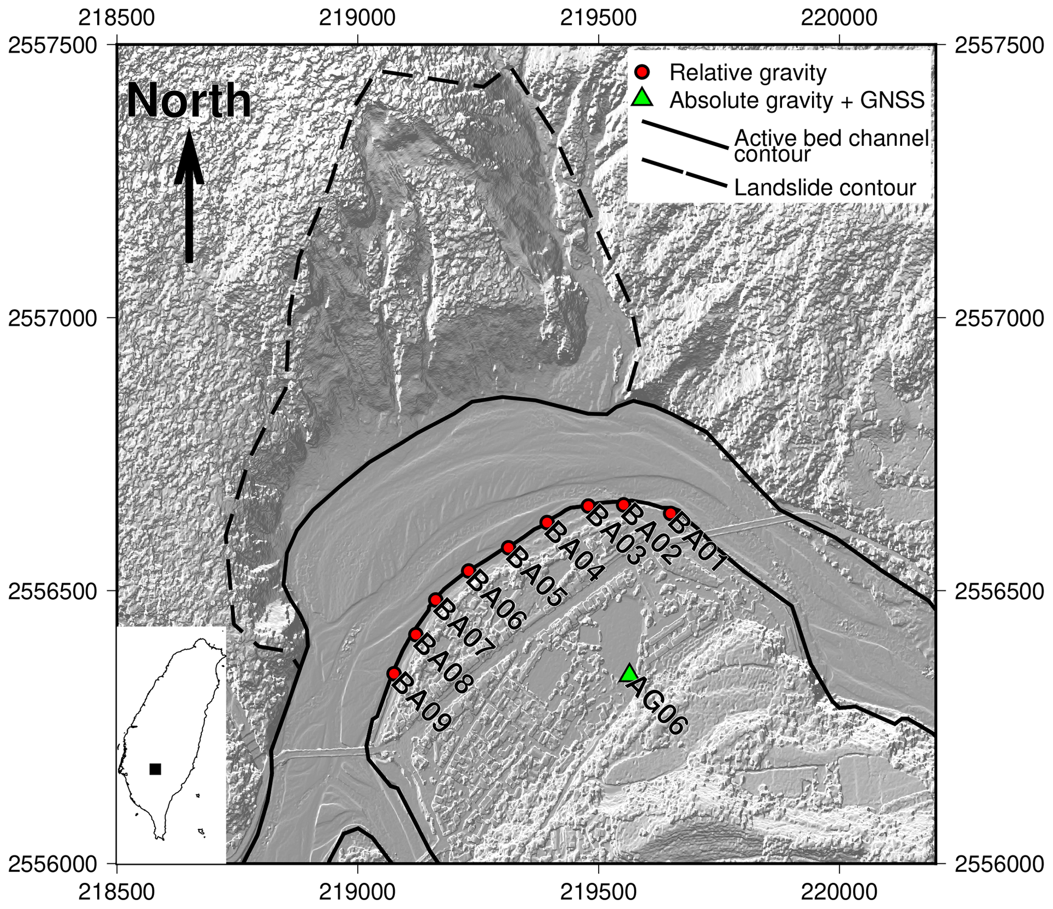
Figure 1 Shaded relief map of the study area. Absolute gravity measurements are performed only at AG06 while relative gravity measurements are performed at every site. The background image is the hill-shaded topography at half-meter resolution obtained by photogrammetry using an unmanned aerial vehicle (UAV). Map to the bottom left shows the study area in Taiwan. Axes are in meters in the TWD97 coordinate reference system.

Time-lapse gravimetry, which is the measure of gravity changes with time at a fixed location, is the only geophysical tool directly sensitive to mass redistributions at and below the earth's surface. It has been widely applied in the fields of glaciology, hydrology and solid earth processes, either from space, with the Gravity Recovery and Climate Experiment (GRACE) mission (Farinotti et al., 2015; Han et al., 2006; Longuevergne et al., 2013; Pail et al., 2015; Tapley et al., 2004), or from terrestrial instruments (Van Camp et al., 2017; Crossley et al., 2013). Recent studies demonstrate the new potential of time-lapse gravity for studying surface processes as well because the mass of deposited or eroded sediment can also significantly alter the gravity field (Liu et al., 2016; Mouyen et al., 2013, 2018). Since gravimetry is presently undergoing a revival thanks to recent technological advances (Ménoret et al., 2018; Middlemiss et al., 2016, 2017), new ranges of applications such as sediment mass quantification offer opportunities to promote the use of gravimetry outside the field of geodesy.

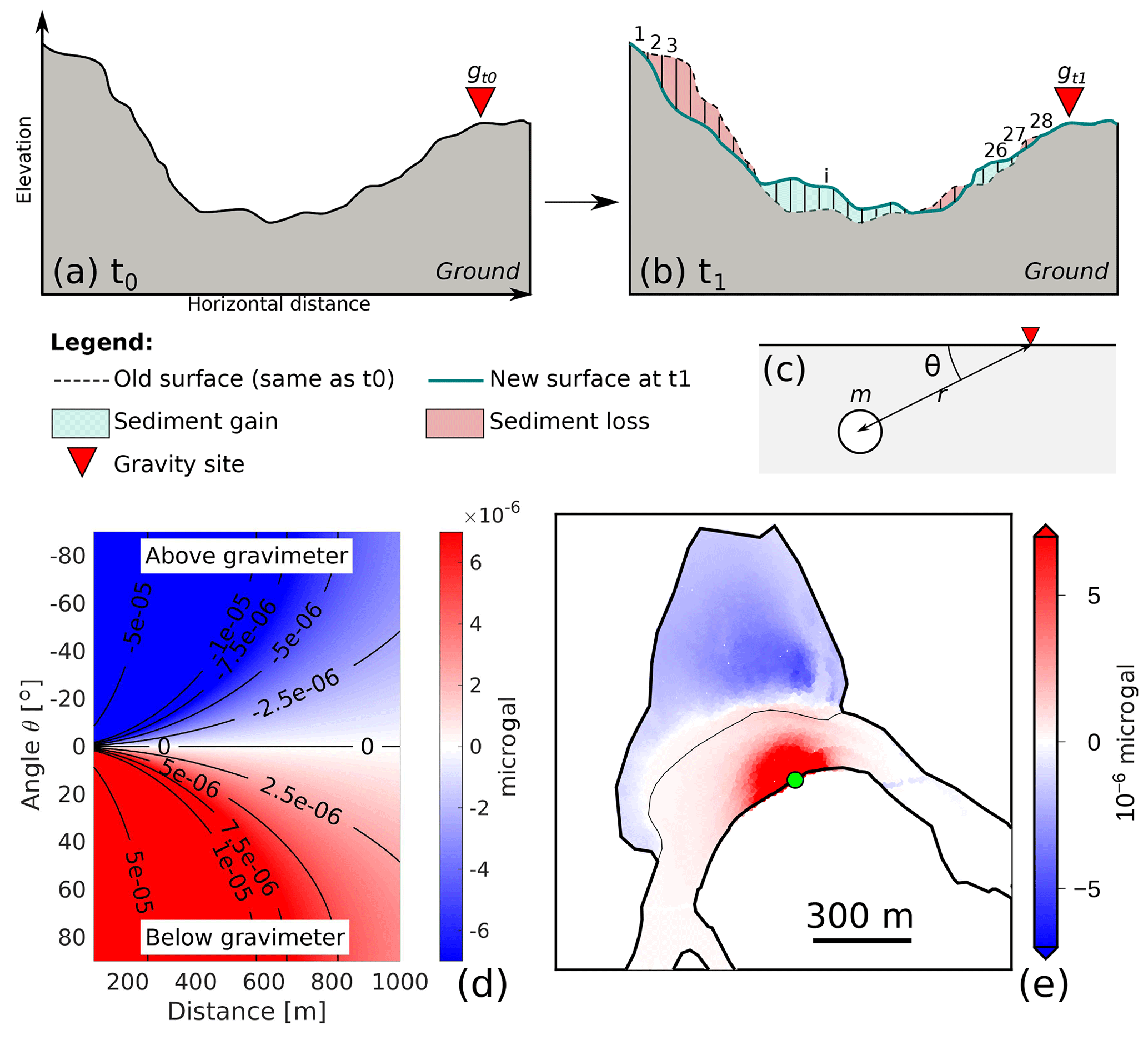
Figure 2 (a) Ground surface elevation at time t₀ when gravity is measured and equal to g_t0. (b) New ground surface at t₁>t₀ after sediment mass redistributions occurred. This mass redistribution is discretized in 28 prisms for the gravity modeling (Eq. 1). The gravity is measured again at the same place and is equal to g_t1. (c) Parameters used for computing a point-mass gravity effect (Eq. 1; point mass means that the element is approximated to a point where the mass is that of the element). (d) Theoretical effect of a 2000 kg point mass as a function of its distance and angle (Eq. 1) from the gravimeter. (e) Synthetic gravity effect at one measurement site (green dot; actually BA04) for each mass element located at the surface of the Paolai riverbed or landslide. A mass element is a 0.5 m × 0.5 m × 1 m rectangular prism of density 2, whose height is given by the actual topography of the area (Fig. 1). The actual gravity effect measured at the green site is the sum of each element of the gravity effect. The color scale is saturated to highlight the change in sign across the landslide area.

The classical limitation for gravimetry is the nonuniqueness of its solutions since gravity changes are integrative and sensitive both to mass variations and to the location where these mass variations take place (Fig. 2 and Eq. 1). Nevertheless, network gravity surveys have shown their high value in estimating belowground mass changes in hydrology (Jacob et al., 2010; Naujoks et al., 2008), volcanology (Carbone and Greco, 2007; Kazama et al., 2015) and reservoir monitoring evolution (Ferguson et al., 2008; Hare et al., 2008). When studying underground processes, especially groundwater, it is common to simplify the redistribution to a 1-D problem. The groundwater level variations Δh are the main observations, and gravity effects are computed using a Bouguer plate (2πGρ_waterΔh). This simplification is necessary because it is usually impossible to monitor lateral groundwater redistribution, and the assumption of little lateral change remains appropriate for homogeneous aquifers. The groundwater level variation can be assumed constant over the entire aquifer. Such an assumption is not valid for surface processes because sediment builds complex 3-D bodies, but sediment mass redistributions occur at the ground's surface; thus, they are accessible to accurate location methods such as photogrammetry (Eltner et al., 2016; Niethammer et al., 2012; Schwab et al., 2008). Combining accurate geometries with gravity variations can thus enable proper mass estimations. Figure 2 illustrates the use of time-variable gravimetry to quantify sediment mass redistribution at the earth's surface. In the simplest case, when considering each ground element as a point mass, the total change in gravity Δg measured between t₀ and t₁ is

$$\begin{array}{}\text{(1)}& \mathrm{\Delta }g=g_{t\mathrm{1}}-g_{t\mathrm{0}}=\sum _{i=\mathrm{1}}^N\mathrm{\Delta }{g}_i={\sum }_{i=\mathrm{1}}^N{\displaystyle \frac{G{m}_i}{r_i^{\mathrm{2}}}}\sin \mathit{\theta },\end{array}$$

where Δg_i is the vertical component of the gravitational change at each element i (i ranging from 1 to N=28 in Fig. 2b) considered as a point mass (Fig. 2c) of mass m_i located at a distance r_i from the gravimeter, and G is the universal gravitational constant. Note that the gravitational attraction of any element decreases with the square of the distance between this element and the site where gravity is measured so that the distance of the mass redistribution can be a strong limiting factor in measuring significant gravity changes. Note also how the angle θ between the point mass and the site where gravity is measured contributes to the gravity effect. The gravity effect is maximum when the point mass is at the vertical of the site, negative if above the site and positive if below. If the point mass is exactly at the horizontal with the gravimetric sensor, then the gravity effect is null. The effects of the angle and the distance are shown in Fig. 2d and e for a general case and for one actual site of the survey, respectively. Point-mass simplification is ideal to grasp the concept of gravimetry, but it is not suitable for the precise quantifications that are the aim of this study. All gravity modeling will thus be done using rectangular prism modeling (Nagy, 1966), which is the most appropriate way to compute the gravity effect of surface changes measured by photogrammetry.

After introducing the study area, we describe the gravimetry and photogrammetry surveys that we conducted, together with our data processing workflow. We then show the results of both methods and interpret them jointly in order to retrieve the mass of sediment redistributed in this area from 2015 to 2017. We eventually discuss the benefits and limitations of this method.

2 Study area

The joint gravimetry–photogrammetry survey was set in southern Taiwan at Paolai village next to the Laonong River (Fig. 1). The gravity network contains one site, AG06, for the absolute gravity (AG) measurement and nine sites, BA01 to BA09, for the relative gravity (RG) measurements. During the 2017 survey, all sites but BA02 were located to centimeter accuracy using the Global Navigation Satellite System (GNSS) enhanced by the real-time kinematic (RTK) technique. The exact location of BA02 could not be measured due to the unexpected storage of concrete blocks, referred to as dolosse (singular: dolos), placed on the river shore to protect it from erosion. This dolos storage also covered BA03 and BA04, but those two sites could still be measured. The gravimetric effect of the dolosse was estimated and removed from the measurements.

The first reason for choosing this location is that time-lapse absolute gravity surveys have been done at AG06 since 2006 in the context of the Absolute Gravity in the Taiwan Orogen (AGTO) project. This project made it possible to measure, for the first time, sediment mass redistribution using time-lapse absolute gravimetry and showed that significant sediment transfers occurred around Paolai (Kao et al., 2017; Mouyen et al., 2013). Indeed, this site experiences vigorous sediment transfer processes powered by heavy rains brought by tropical cyclones (typhoons) and monsoonal events, especially in May to August (Chen and Chen, 2003). The heavy rains destabilize the slopes of the high Taiwanese mountains, triggering landslides and debris flows (Chiang and Chang, 2011). This occurs on a regular basis: five to six typhoons make landfall in Taiwan every year (Tu et al., 2009), mostly between May and September. The most remarkable event was Typhoon Morakot in 2009, which produced the worst flooding in the last 60 years in Taiwan and up to 2777 mm of accumulated rainfall (Ge et al., 2010) and triggered 22 705 landslides with a total area of 274 km² (Lin et al., 2011). Landsliding, which can also be triggered by regional active tectonics, is the main process supplying sediment to rivers in Taiwan (Dadson et al., 2003; Hovius et al., 2000).

The second reason for choosing this location is practical. This location offers a stabilized path made of concrete on the southern bank of the Laonong River, where the relative gravity benchmarks could be properly set on stable and sustainable sites which were easily accessible for measurements. Also, a continuous GNSS station, PAOL (lat 23.10862^∘, long 120.70287^∘; elevation 431 m), is colocated with the AG06 pillar and is maintained by the Institute of Earth Sciences, Academia Sinica (IES-AS, 2015). This makes it possible to precisely take into account gravity changes due only to ground vertical displacements.

In this area, both the Laonong River and the landslide (Fig. 1) are susceptible to sediment transfers. The gravimetry–photogrammetry survey is set up to focus on these processes. Note that what we call the river (plain black line contour in Fig. 1) is the active channel bed that includes emerged alluvia. During yearly measurements, the water extent of the river only covers a fraction of this area, even if the period 2015–2017 saw some higher water levels and larger extents, especially during large floods.

3 Methods

This section introduces the two main methods used in this study: gravimetry and photogrammetry. Gravimetry is sensitive to masses and their distribution, while photogrammetry is here a geometric measure of the ground surface and hence of the sediment distribution. Therefore, combining gravimetry and photogrammetry removes the geometric ambiguity inherent to gravity measurements and allows us to focus on sediment masses. This combination is done through a least squares inversion to determine sediment density, which is a mass per unit of volume.

3.1 Time-variable gravimetry

Gravity was measured at 10 sites (Fig. 1) in 2015, 2016 and 2017 and always over 2 d in November since the climatic conditions during this month are usually suitable for gravimetry fieldwork (e.g., no typhoon or heavy rains, reasonable temperatures). By measuring gravity during the same period of each year, we also expect to minimize hydrological effects, which have a strong annual periodicity in this area (Chen and Chen, 2003). Absolute and relative gravity surveys were done in parallel on the same days.

Relative gravity measurements were done using a Scintrex CG-5 AutoGrav (serial number 167). The measurement principle is to assess length variations of a spring holding a proof mass between different times and places, using a capacitive displacement transducer, and to convert them into gravity variations (Scintrex Ltd., 2010). The instrument is leveled at each site and repeats 90 s measurements continuously. We stop measurements when gravity readings repeat within 3 µGal (1 µGal = 10⁻⁸ m s⁻²) while the internal sensor temperature remains stable. This usually takes 10 to 15 measurements, which is 15 to 23 min, although up to 25 measurements were required in some rare cases. Only the later measurements, when gravity readings are stable, are used in the gravity network adjustment to estimate the drift. Indeed, relative gravimeter measurements are subjected to an instrumental drift, which is corrected using the software Gravnet (Hwang et al., 2002). Inferring this drift requires remeasuring one or more sites within a few hours. In this study, all surveys start and end at AG06, which is also revisited up to four times during the survey, together with other relative gravity sites (Appendix A). In addition, ambient temperature alters gravity measurements at a rate of −0.5 $\mathrm{\mu }\mathrm{Gal}{}^{\circ }{\mathrm{C}}^{-\mathrm{1}}$ (Fores et al., 2017). This effect was taken into account before adjusting the instrumental drift of the gravimeter.

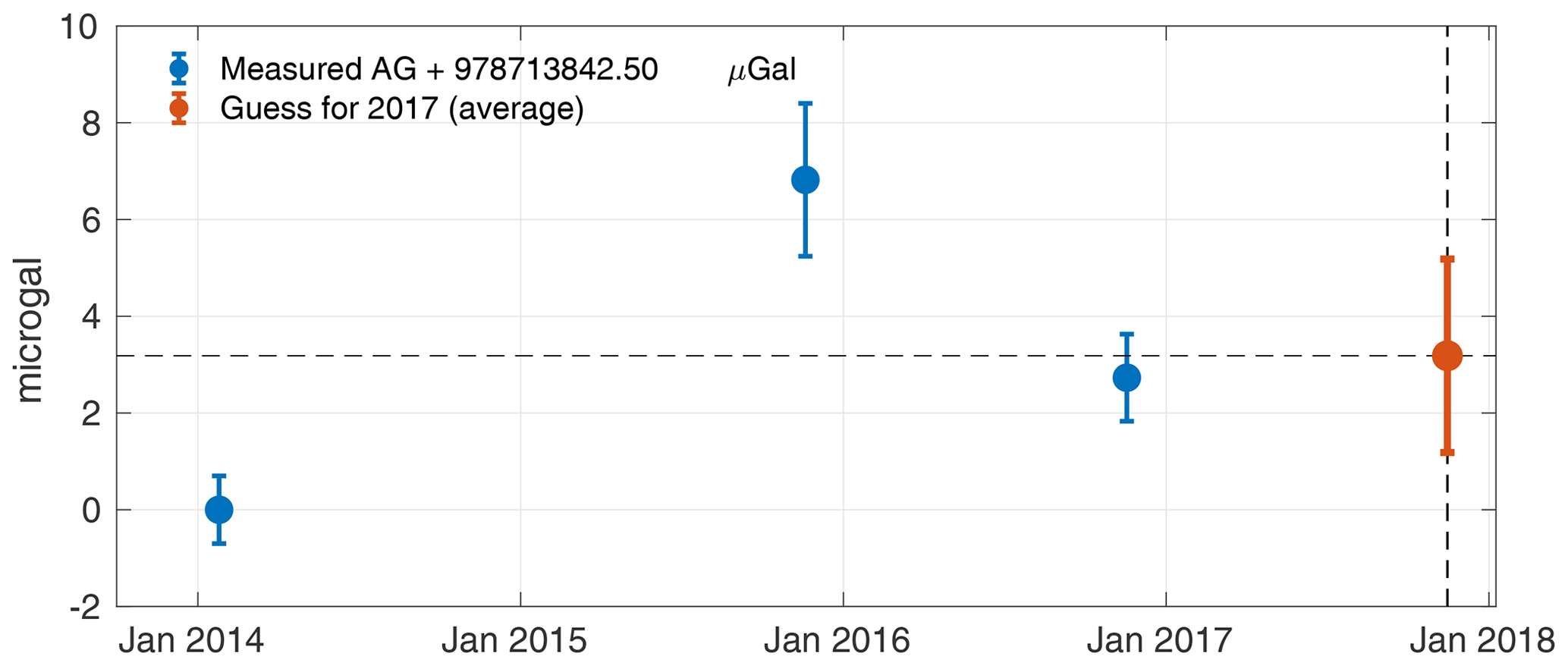
Figure 3 Absolute gravity values measured at AG06 in 2014 (25 January), 2015 (20 November) and 2016 (18 November). In 2017 (16 November), the absolute gravimeter suffered from a laser problem, and no measurement could be done. We thus assume that the value in 2017 is the average of the 2014, 2015 and 2016 values. These absolute gravity values are already corrected for tides, air pressure and polar motions but not for hydrology or vertical ground displacements. The error bars for the values in 2014, 2015 and 2016 combine the measurement uncertainty obtained during each gravity survey and the uncertainties due to the tides, air pressure and polar motion corrections.

The absolute gravity measurements were done using a Micro-g FG5 (serial number 224), which monitors the drop of a free-falling corner cube in a vacuum. During its free fall, the positions and times of the corner cube are precisely assessed using laser interferometry and an atomic clock (Niebauer, 2015; Niebauer et al., 1995). One measurement takes ∼ 12 h and consists of 24 sets of 100 test mass drops starting every 30 min (one drop every 10 s). Measurements are always done overnight, when anthropogenic seismic noise and temperature variations are lower than during daytime. A laser problem in the FG5 prevented us from measuring absolute gravity in 2017. This is compromising since the measurements at BA01–BA09 need an absolute reference to be compared with the previous survey in 2016 at these sites. In order to interpret the 2017 relative gravity survey, we decide to estimate the AG06 absolute gravity value in 2017 as the mean of the values measured in 2014, 2015 and 2016, which is 978 713 845.1 ± 3 µGal (Fig. 3). We believe this is a reasonable approach because there were no major climate or tectonic events between November 2016 and November 2017 around the Paolai region. In addition, by repeating the gravity surveys at the same time of the year, in November, the gravity difference due to hydrological changes is at the microgal level, which is about the size of the errors in the relative gravity measurements. The hydrological conditions are described in more detail in the next paragraphs. For the 2017 estimated absolute gravity value, we arbitrarily set the SD to a value about 3 times larger than usual at this site. The AG06 values in 2016 and 2017 are quite similar, less than 0.5 µGal difference. Although absolute gravity measurements at AG06 started in 2006 and repeated once a year except from 2011 to 2013, it is not possible to use these older data for the estimation of the 2017 value. Indeed, in 2009, Typhoon Morakot and its subsequent massive landslides reset the whole area. The gravity offset between November 2008 and November 2009, i.e., before and after Typhoon Morakot, is about 30 µGal and is due to large sediment redistribution in this area (Mouyen et al., 2013). Sediment redistribution due to Typhoon Morakot was such an exceptional event, with a significant impact on gravity, that it cannot be included in the extrapolation of the 2017 gravity value. The measurements from 2009 to 2010 were not used either because too much reconstruction work was ongoing at that time, taking out debris from the river and thus interfering with natural sediment redistribution.

Table 1 Summary of the corrections applied to our gravity measurements with their order of magnitude and a statement on whether they are applied before or after the drift adjustment. The uncertainties of the first four corrections are those proposed by Van Camp et al. (2005). See text for the methods' references.

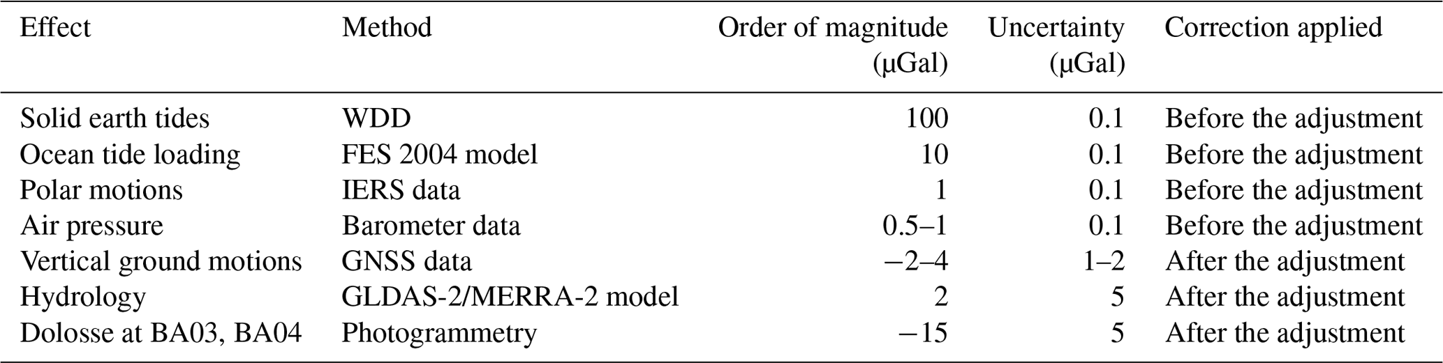
To focus on sediment mass redistribution, other sources responsible for gravity changes must be removed from the gravity time series. Here, these effects are the tides, air pressure variations, polar motions, vertical ground motions and hydrology. These corrections are detailed in the next paragraph and summarized in Table 1.

Solid earth tides are computed with TSoft (Van Camp and Vauterin, 2005) using the tidal parameters from Dehant et al. (1999) referred to as WDD. Ocean tide loading effects are computed using the FES2004 model (Lyard et al., 2006) with the ocean tide loading provider (Bos and Scherneck, 2003). Polar motion effects are computed using the International Earth Rotation and Reference Systems Service's parameters and the absolute observations data processing standards (Boedecker, 1988). Atmospheric effects, that is to say gravity changes due to air masses, are corrected using local barometric records done at a continuous weather station located ∼ 12 km west of Paolai (station C0V250) and an admittance factor of −0.3 µGal hPa⁻¹ (Merriam, 1992). Solid Earth tides, ocean tide loading and atmosphere loading are corrected before the drift adjustment of the relative gravity measurements because they can have significant effects over a few hours, that is to say while the relative gravity survey is being done. Not correcting them would bias the drift estimation by mixing gravity changes due to the instrumental drift with those due to tides and atmosphere. Vertical displacements of the ground also change the gravity because the gravity measured at any place on the Earth's surface depends on the inverse of the square of the distance between this site and the Earth's center of mass. Therefore, if the site is uplifting (further from the center of mass) or subsiding (closer to the center of mass), it will have a lower or higher gravity value, respectively. This effect is corrected using continuous GNSS time series recorded at AG06 (the GNSS site, PAOL, is colocated with AG06; Fig. 4) and assuming a theoretical ratio Δg∕Δz = −2 µGal cm⁻¹ (Van Camp et al., 2011), where Δg is the gravity change and Δz is the elevation change at the same location. Between 2015 and 2017, the ground uplift at AG06 is about 1.3 cm yr⁻¹. That is a large uplift rate, explained by the active mountain building processes at work in Taiwan, where an uplift of up to 1.9 cm yr⁻¹ is measured (Ching et al., 2011). Although the relative gravity sites are between 300 and 500 m from the PAOL permanent GNSS, we apply the same uplift correction to these sites as to AG06. Indeed, tectonic uplift is a regional feature and can be assumed constant over a few hundred meters unless an active fault or more cross the area, but there is no evidence for such a fault in Paolai.

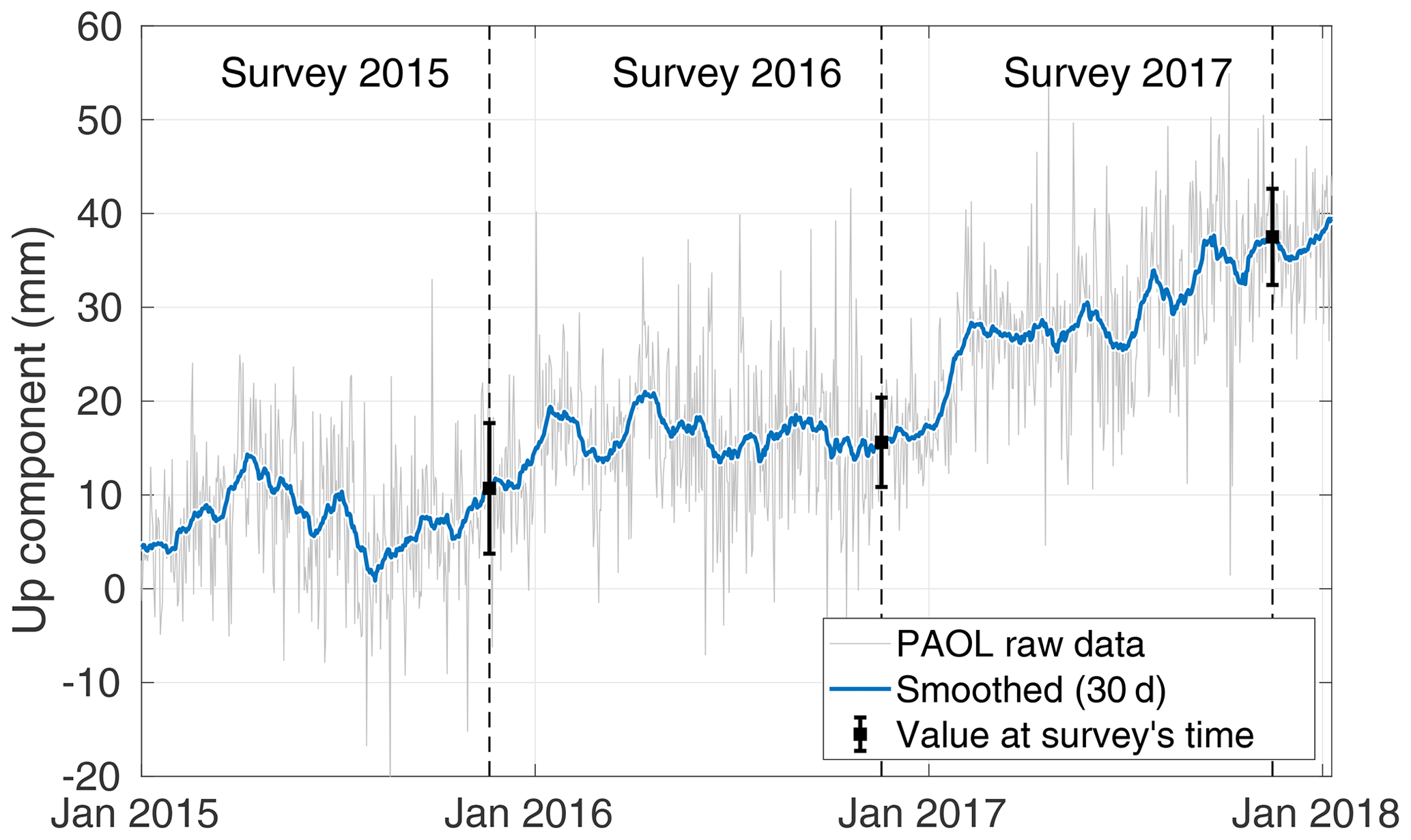
Figure 4 Ground vertical displacement time series at the PAOL GNSS station, colocated with AG06, provided by the GPSLAB database (IES-AS, 2015). Solutions are computed in the IGS08 reference frame (Rebischung et al., 2012). The time of each joint gravimetry–photogrammetry survey is shown by dotted lines. The error bar is computed from the SD of the measurements of the same 30 d window.

We also correct the effect of hydrology, which deforms the earth surface at the global scale and changes the groundwater mass attraction at local scales, near the gravimeter. This correction relies on global hydrological models. We consider two of them in this study:

1. the Global Land Data Assimilation System version 2 (GLDAS-2) forcing the Noah land surface model (Rodell et al., 2004);

2. the Modern-Era Retrospective analysis for Research and Applications version 2 (MERRA-2; Gelaro et al., 2017).

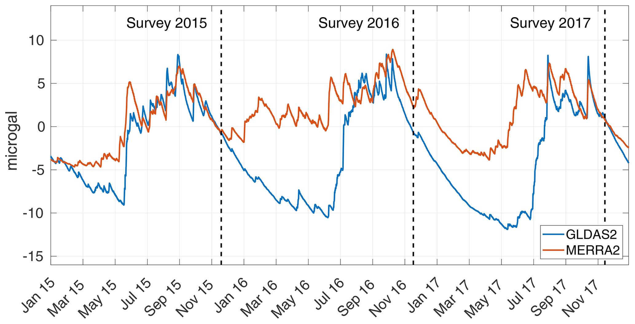
Figure 5 Hydrological effect on gravity at AG06, estimated from global hydrological models GLDAS2 and MERRA2.

The gravitational effect due to each of these models is provided by the EOST loading service (Boy, 2015; Petrov and Boy, 2004). Unlike the other corrections, the hydrological correction may suffer large uncertainties because of (1) the complexity of hydrological processes, (2) the difficulty of measuring groundwater and (3) its large effect on gravity (Jacob et al., 2009; Longuevergne et al., 2009; Pfeffer et al., 2013). Indeed, the effects of GLDAS-2 and MERRA-2 on gravity predict up to 20 µGal of seasonal amplitude in the hydrological signal with sometimes large differences up to 10 µGal between the different models (Fig. 5). Nevertheless, surveying in November appears to be a valuable way of decreasing the hydrological impact on the gravity data, since this effect is lower than 3 µGal when considering either of the two hydrological models. We use the average hydrological effect from GLDAS-2 and MERRA-2. We arbitrarily set an uncertainty of 5 µGal to this correction (Table 1) to account for possible bias in the models.

We also correct the effect of the set of dolosse in 2017, which is only significant at BA03 and BA04. These structures, located above BA03 and BA04, were responsible for an artificial decrease in gravity of about 15 µGal. Their gravitational effect is computed using the dolosse's geometry measured by the photogrammetry and rectangular prism method (computation details in Appendix B). Given the uncertainty of this correction process, we add an arbitrary 5 µGal uncertainty to the gravity changes measured at BA03 and BA04 during the 2017 survey.

The last non-sediment effect on gravity is the actual Laonong River: water density ρ_w = 10³ kg m⁻³. The photogrammetry measures the river surface but not its depth. Also, at each survey, the river did not follow the same path across the active riverbed. Therefore, neither the volume of the river nor its variation can be estimated, which prevents us from obtaining a gravity correction for the river.

3.2 Photogrammetry

The purpose of the photogrammetry survey is to generate high-resolution digital surface models (DSMs) in 2015, 2016 and 2017 at the moment of the gravity surveys to quantify the sediment volume changes between each survey.

3.2.1 Equipment

The photogrammetry survey was done with an unmanned aerial vehicle (UAV), commonly known as a drone, which is commonly used in morphotectonic studies (Chang et al., 2018; Deffontaines et al., 2017, 2018). The UAV is a modified, currently available Skywalker X8 fixed-wing aircraft reinforced by carbon fiber rods and Kevlar fiber sheets (Fig. 6a and b). To generate a high-resolution DSM, orthorectified mosaic images and a true 3-D model, the UAV is equipped with a Sony ILCE-QX1 global shutter camera and a 16 mm SEL16F2.8 lens.

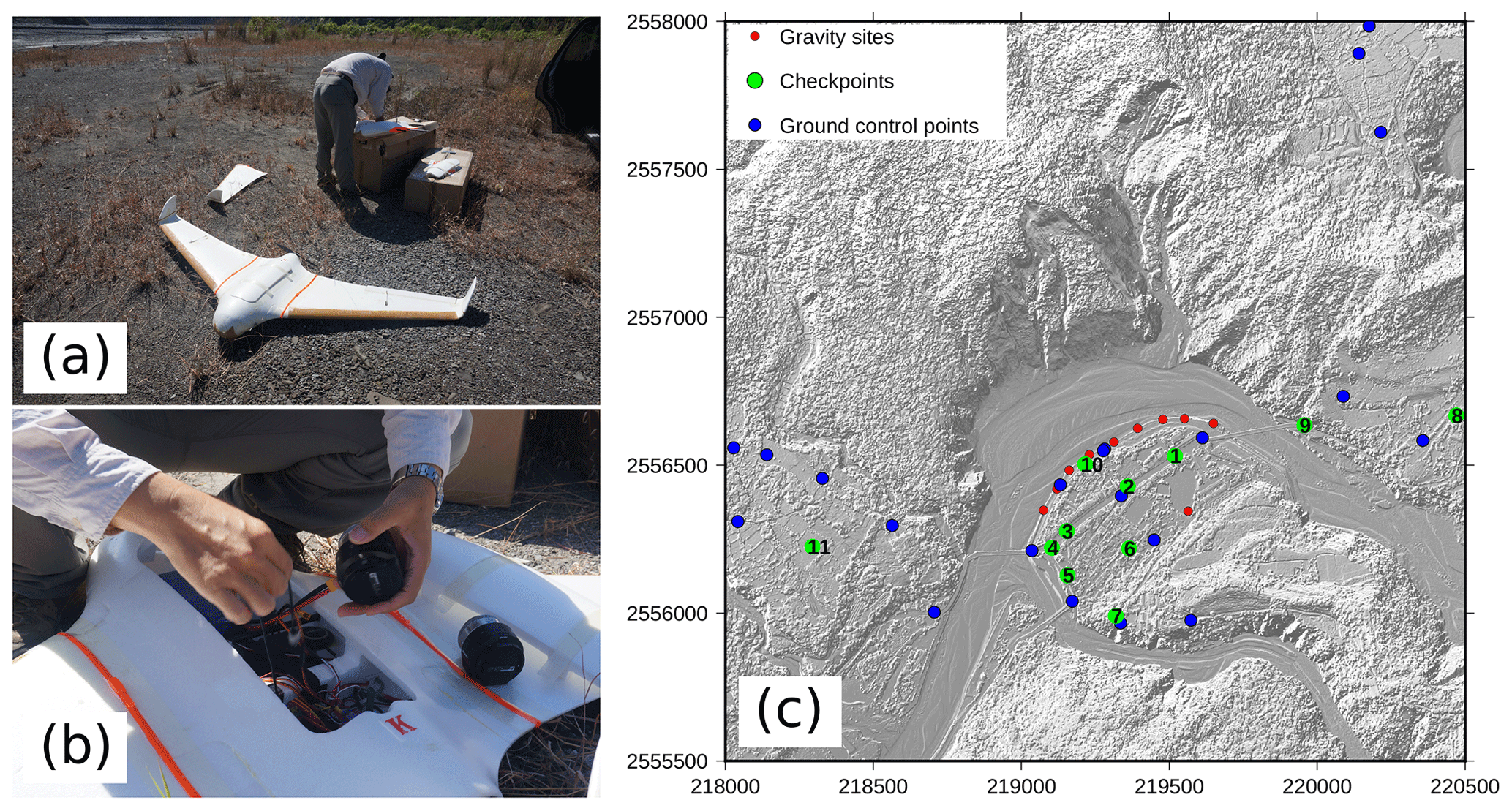
Figure 6 (a) Modified Skywalker X8 UAV. (b) Close-up on the central compartment of the UAV, where the camera and lens are mounted. (c) Map of the ground control points and checkpoints (numbered according to Table 4) with the shaded topography in the background. The gravity sites are also shown for reference.

3.2.2 Survey design and execution

The UAV is launched by hand, then flies, takes photos and lands autonomously using a preprogrammed flight plan. The autopilot system is composed and modified from the open-source APM (ArduPilot Mega 2.6 autopilot) firmware and open-source software Mission Planner (Oborne, 2010), transmitted by ground–air XBee radio telemetry.

Table 2 Image processing summary.

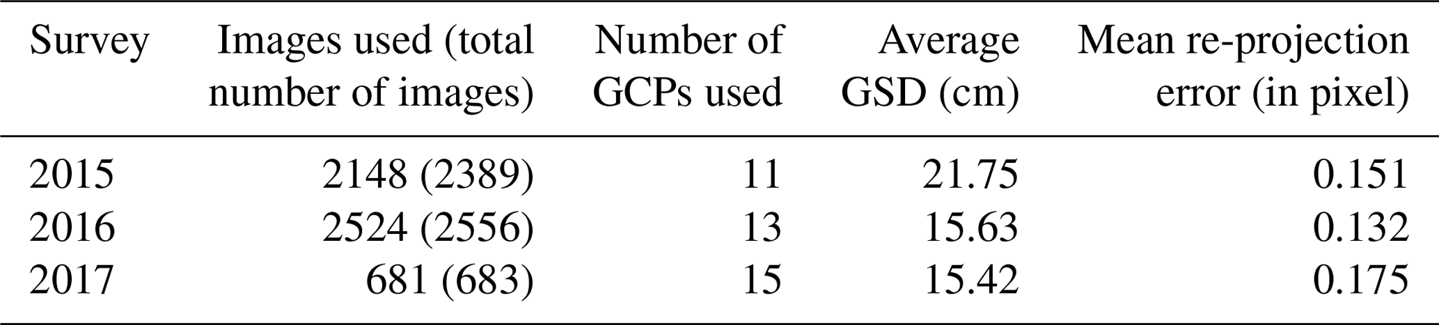
The UAV was flown between 300 and 500 m above ground level. It covered an area of about 15–20 km² with about 15–20 cm ground sampling distance (GSD) in one single flight mission (Table 2). Repeated adjacent photographs were kept for at least 85 % endlap and 50 % sidelap. The GPS location of the acquired image is recorded in the autopilot log. Each UAV flight mission took about 90 min. On average 13 ground control points (GCPs) per survey and 11 checkpoints (CKPs) were measured in the field to control and verify the quality of the datasets (Fig. 6c). The GCPs are preexisting or painted benchmarks on the ground. The CKPs are permanent features such as bricks with patterns, road signs and crosswalks. The GCP and CKP coordinates were measured by virtual base station (VBS) RTK GPS and RTK GPS at least 3 times each. The mean vertical error and the root mean square are 1.5 and 4.2 cm, respectively.

3.2.3 Photogrammetry processing and results

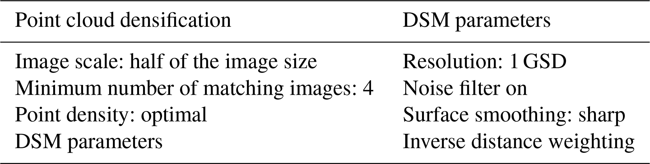
The images acquired by the UAV, their positions and the GCP positions are processed using Pix4Dmapper (Pix4D, 2020) in order to generate a DSM with a grid spacing of 50 cm based on multi-view stereo, which aims at reconstructing a complete 3-D object model from a collection of images taken from known camera viewpoints (Furukawa and Ponce, 2010; Seitz et al., 2006). Images and camera parameters such as focal length, principal point, radial distortion, tangential distortion, aspect ratio and skew are auto-adjusted for each image during processing. The point cloud densification and DSM parameters set specifically for Pix4Dmapper are summarized in Table 3.

Table 3 Processing parameters set in Pix4D.

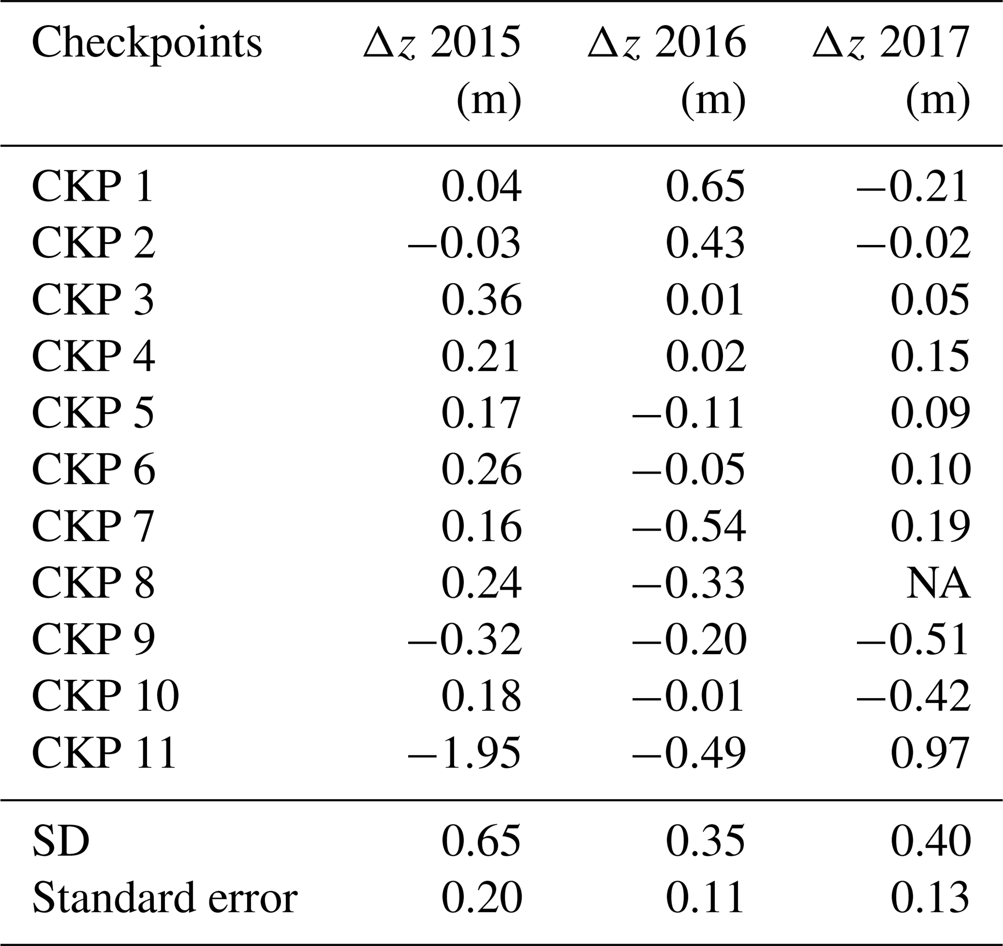
The quality of the DSM is calculated by comparing its elevation with that of the CKP at the same coordinates. The error of the dataset is denoted in Table 4, where the data show that the mean of the error compared with the field survey is about 0.11–0.20 m with an SD of 0.334–0.622 m.

Table 4 Results of field checkpoints and the elevation difference (Δz) of photogrammetric DSM for each survey. NA = not available.

4 Survey results

The results of the gravimetry and photogrammetric surveys are summarized in Fig. 7 and Table 5. The largest gravity changes occurred between 2015 and 2016, with most sites showing an increase of more than 30 µGal. In contrast, the gravity decreased at most sites from 2016 to 2017. When measured above the redistributed masses, increase and decrease in gravity correspond to gain and loss of masses, respectively. Qualitatively, this is in agreement with the corresponding changes observed in the digital surface models (DSMs) in the active bed channel, showing higher sediment thicknesses, thus a gain of mass, from 2015 to 2016 and large surfaces of lower sediment thicknesses from 2016 to 2017. Over the time period 2015–2016, the top of the landslide is actively eroded, up to 46 m, while its toe displays significant sedimentation up to 33 m. The active riverbed shows a mixed pattern of erosion and sedimentation between −1.19 and 1.21 m on average, possibly resulting from the migration of the river braids. In contrast, over the time period 2016–2017, the landslide displays mostly erosion, up to 39 m, while the riverbed continues to display a mixed pattern of erosion and sedimentation between −1.17 and 1.08 m on average.

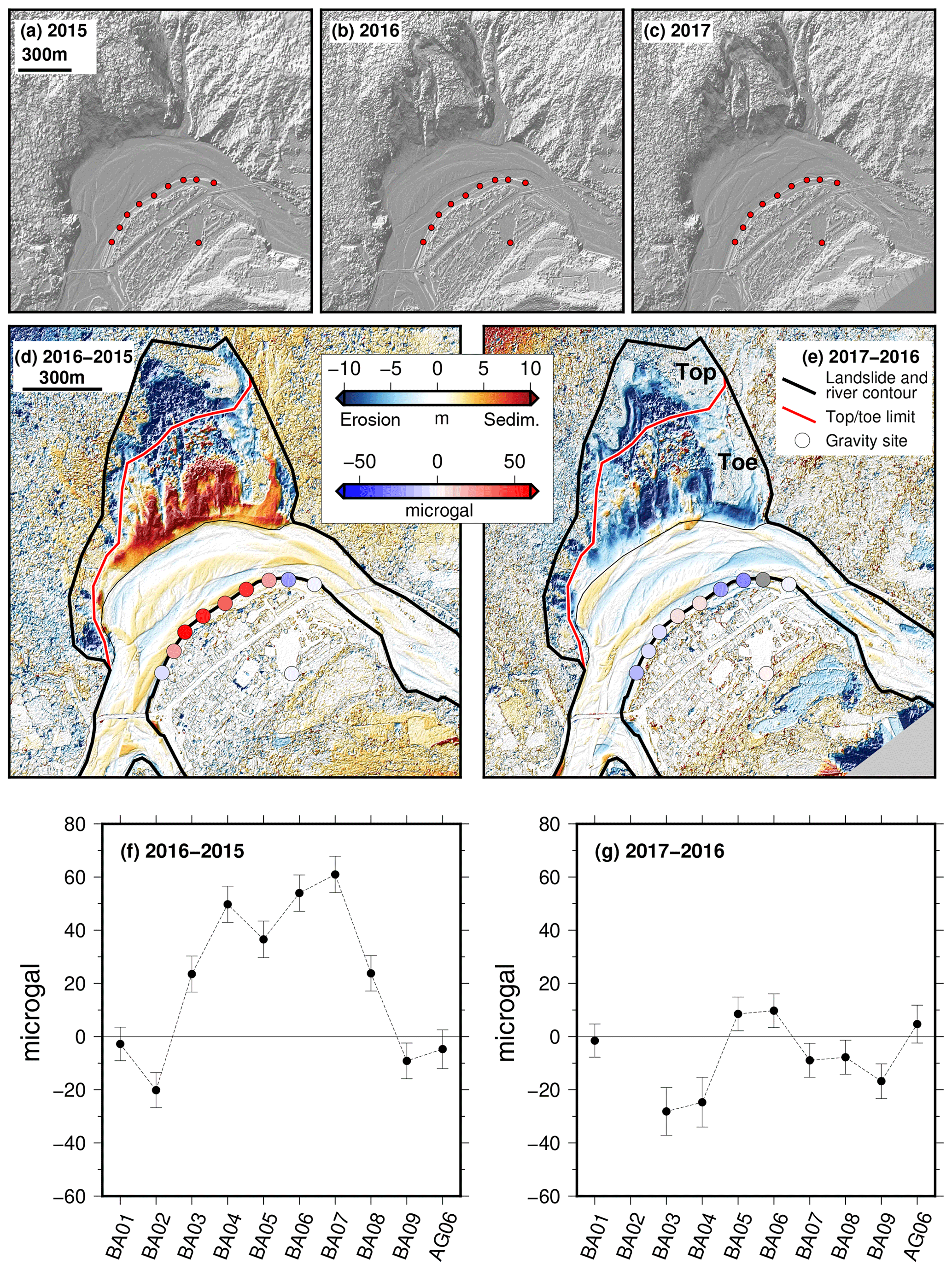
Figure 7 The digital surface models in (a) 2015, (b) 2016 and (c) 2017 and their differences (d) between 2016 and 2015 and (e) between 2017 and 2016. The disks that locate the gravity sites are colored relative to the gravity change. The black contour line delimits the river and the landsliding area. The landsliding area is divided into two parts: the top and the toe. The color scale of the elevation changes is bounded within ± 10 m, which contains 92 % of the elevation changes between 2015 and 2016 and 96 % of the elevation changes between 2016 and 2017. The extrema are −46 m and 33 m between 2015 and 2016 and −38 m and 33 m between 2016 and 2017. (f) Gravity changes between 2015 and 2016. (g) Gravity changes between 2016 and 2017. BA02 could not be measured in 2017 because of ongoing construction work near the site. The error bars represent $\surd {\sum }_i{\mathit{\sigma }}_i^{\mathrm{2}}$, where σ is the uncertainty of the gravity measurements after the instrumental drift adjustment and the seven corrections given in Table 1 (thus i ranges from 1 to 8).

Table 5 Gravity values measured at each site for all surveys (in µGal). The values at each relative gravity site (BA) are given relative to the absolute value measured at AG06.

The gravimetric and photogrammetric techniques show large changes in gravity and topography, which demonstrate active processes of sediment mass redistribution in the river and on the slow landslide. In the next section, we combine these results to assess the mass of sediment redistributed from 2015 to 2017. Note that we focus the DSM analysis on the area bounded by the black line in Fig. 7d and e, which is restricted to the landsliding zone and the river.

5 Joint analyses of the gravity and photogrammetry data

Using the DSM, we build rectangular prisms with horizontal sides of 0.5 m, i.e., at the scale of the DSM resolution, and a vertical side as high as the elevation at the time of the corresponding surveys, i.e., bottom at 0 m and top at the surface elevation. Among the three (2015, 2016 and 2107) photogrammetry surveys, the 2017 survey has the smallest surface extent. Its limits are thus used to cut the 2015 and 2016 photogrammetric survey areas so that all DSMs cover the exact same area. The total mass of redistributed sediment equals the change in volume between each survey multiplied by the density of the sediment. We use the gravity data to assess this density using an inverse modeling approach. Note that since gravity decreases with the square of the distance between the measurement site and the mass location, we can bound our analysis to the area covered by the photogrammetry surveys without biassing the analysis. Indeed, using the wider 2015 and 2016 survey coverages, we find that extending our working area in the north–south and east–west directions by steps of 100 m does not alter the gravity changes computed at each site by more than 1 %.

We design three inversion cases to retrieve the densities of the redistributed materials, using a least squares criterion. These cases are independent of each other and aim at increasing the amount of possible different densities for comparison. Thus we invert the following:

• Case 1 – the average density ρ of the material redistributed during the surveys;

• Case 2 – the density of the sediment in the river ρ_r and the density ρ_l of the material in the landslide;

• Case 3 – the density of the sediment in the river ${\mathit{\rho }}_{\mathrm{r}}^{\mathrm{1615}}$ from 2015 to 2016 and ${\mathit{\rho }}_{\mathrm{r}}^{\mathrm{1716}}$ from 2016 to 2017 and the density ρ_l of the material in the landslide.

Here we will solve an overdetermined problem, where we have more observations (20 gravity differences over the 3 years) than variables to estimate (density, three at most, in Case 3). However, gravity observations are too few and unevenly distributed over the study area to try to invert the density at each pixel (more than 4 million) of the photogrammetry survey. In practice, the matrix representation of this system is (e.g., Hwang et al., 2002)

$$\begin{array}{}\text{(2)}& \mathit{L}+\mathit{V}=\mathbf{A}\mathit{X},\end{array}$$

where the design matrix A, vector of unknowns X and vector of observations L are defined as

$$\begin{array}{}\text{(3)}& {\displaystyle }& {\displaystyle }\mathbf{A}=\left[\begin{array}{ccc}\mathrm{d}{g}_{\text{mod},\mathrm{r}}^{\mathrm{1615},\text{BA01}}& \mathrm{0}& \mathrm{d}{g}_{\text{mod},\mathrm{l}}^{\mathrm{1615},\text{BA01}}\\ \mathrm{⋮}& \mathrm{⋮}& \mathrm{⋮}\\ \mathrm{d}{g}_{\text{mod},\mathrm{r}}^{\mathrm{1615},\text{AG06}}& \mathrm{0}& \mathrm{d}{g}_{\text{mod},\mathrm{l}}^{\mathrm{1615},\text{AG06}}\\ \mathrm{0}& \mathrm{d}{g}_{\text{mod},\mathrm{r}}^{\mathrm{1716},\text{BA01}}& \mathrm{d}{g}_{\text{mod},\mathrm{l}}^{\mathrm{1716},\text{BA01}}\\ \mathrm{⋮}& \mathrm{⋮}& \mathrm{⋮}\\ \mathrm{0}& \mathrm{d}{g}_{\text{mod},\mathrm{r}}^{\mathrm{1716},\text{AG06}}& \mathrm{d}{g}_{\text{mod},\mathrm{l}}^{\mathrm{1716},\text{AG06}}\end{array}\right],\text{(4)}& {\displaystyle }& {\displaystyle }\mathit{X}=\left[\begin{array}{c}{\mathit{\rho }}_{\mathrm{r}}^{\mathrm{1615}}\\ {\mathit{\rho }}_{\mathrm{r}}^{\mathrm{1716}}\\ {\mathit{\rho }}_{\mathrm{l}}\end{array}\right],\text{(5)}& {\displaystyle }& {\displaystyle }\mathit{L}=\left[\begin{array}{l}\begin{array}{c}\mathrm{d}{g}_{\text{obs}}^{\mathrm{1615},\text{BA01}}\\ \mathrm{⋮}\\ \mathrm{d}{g}_{\text{obs}}^{\mathrm{1615},\text{AG06}}\\ \mathrm{d}{g}_{\text{obs}}^{\mathrm{1716},\text{BA01}}\\ \mathrm{⋮}\end{array}\\ \mathrm{d}{g}_{\text{obs}}^{\mathrm{1716},\text{AG06}}\end{array}\right],\end{array}$$

and V is the vector of residuals (X and V are to be determined by the least squares method). In matrices A and L, dg is the gravity variation that is modeled (dg_mod) or observed (dg_obs) between 2016 and 2015 (1615) or between 2017 and 2016 (1716) at every site (BA01–AG06). The modeled gravity change can be computed for the material in the river (dg_mod,r) or in the landsliding zone (dg_mod,l). This matrix representation is given for the inversion Case 3 and can be simplified for cases 1 and 2.

The design matrix A is built thanks to the photogrammetry surveys, from which we identify the river and the landslides, as well as their respective volume changes. Therefore, knowing also the position of the gravity sites, we compute each element of A using gravity modeling by rectangular prism methods (Nagy, 1966) and an arbitrary density equal to 1. The actual density can be inverted by

$$\begin{array}{}\text{(6)}& \mathit{X}={\left({\mathbf{A}}^{\mathrm{T}}\mathbf{PA}\right)}^{-\mathrm{1}}\left({\mathbf{A}}^{\mathrm{T}}\mathbf{P}\mathit{L}\right),\end{array}$$

where A^T is the transpose of A. The weight matrix P is diagonal, and its elements are the inverse of the gravity uncertainties at each site i. The residuals $\mathit{V}=\mathbf{A}\mathit{X}-\mathit{L}$ are used to compute a posteriori variance of the unit weight:

$$\begin{array}{}\text{(7)}& {\mathit{\sigma }}_{\mathrm{0}}^{\mathrm{2}}={\mathit{V}}^{\mathrm{T}}\mathbf{P}\mathit{V}/(n-u),\end{array}$$

where n is the number of gravity observations and u the number of unknown densities. The uncertainties of the inverted densities are the square root of the diagonal element of the a posteriori covariance matrix of X:

$$\begin{array}{}\text{(8)}& C_{\mathit{X}}={\mathit{\sigma }}_{\mathrm{0}}^{\mathrm{2}}{\left({\mathbf{A}}^{\mathrm{T}}\mathbf{PA}\right)}^{-\mathrm{1}}.\end{array}$$

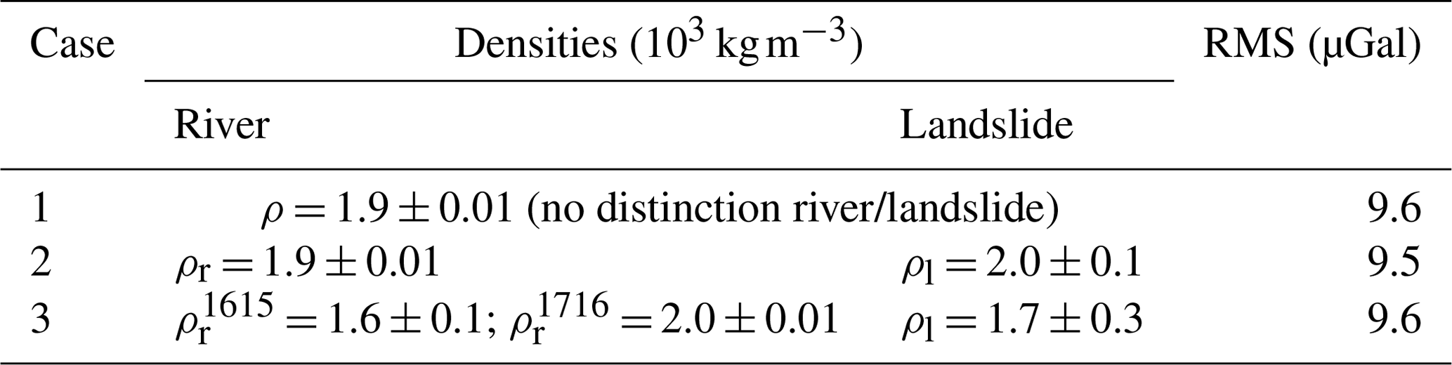
The inverted densities for each case are summarized in Table 6. Cases 1 and 2 return similar densities. Case 3 returns a noticeable difference between the densities of the sediment in the active bed channel for the 2015/2016 and 2016/2017 surveys. A first hypothesis for this difference could be that the composition of the redistributed sediment has changed over the years of the study, for instance because material comes from landslides that occurred in terrain with different densities. A second hypothesis is that the water content of the sediment varies, changing the effective density of the sediment as measured by the gravimeters. We do not have enough data to favor one of these hypotheses, but we will discuss the possible influence of water on our density estimates in Sect. 6.1. Uncertainties on the landsliding material densities (cases 2 and 3) are higher than those of the river sediment, likely because they are further from the gravity sites than the river sediment. As seen in Eq. (1), the further the redistributed masses are, the lower their gravitational effects are.

Table 6 Densities obtained for each inversion case with their SD and the root mean square of the residuals V.

We described in Sect. 3.1 the impossibility of removing the effect of the Laonong River (water) from gravity changes due only to sediment redistribution. As a workaround, here we simply assume a constant river depth of 1 m, which corresponds to rough field estimates. Then, we map the surface limits of the river from the optical images taken by the UAV during each survey. The height h of the river surface is given by the photogrammetry results. The river is then divided into prisms covering the river area with sides of 0.5 m, upper face at elevation h and lower face at elevation h−1 since the river is 1 m deep. We then compute the gravity effect of the river at each site of the network (except BA02, whose position is unknown). This effect is removed from the gravity observation, and the average density inversion (Case 1) is run, giving ρ=1.7 ± 0.1 × 10³ kg m⁻³ and RMS = 9.7 µGal. This represents a decrease of 11 % relative to the density ρ=1.9 ± 0.1 × 10³ kg m⁻³ given in Table 1 and also relative to the mass budget in Fig. 10. These values are to be taken with caution since we do not know the exact geometry of the river, its depth in particular. In the rest of the study, we will only work with the density given in Table 1.

For comparison, during the 2017 survey, we evaluate the in situ densities of the materials in the active riverbed and at the bottom of the landslide at 22 sites (Fig. 8) also using photogrammetry (Appendix C). Estimating in situ density is time-consuming and demanding. It is done here only for comparison purposes; it is not required for the inversion. Indeed, joint gravimetry–photogrammetry estimates an average in situ density over the surveyed area. In contrast, in situ density measurements are done at discrete locations over an area made of heterogeneous material. The in situ densities range from 1.2 to 2.7 × 10³ kg m⁻³ and are spatially heterogeneous, illustrating the variety of materials carried by the river and the landslide. Despite the limited and spatially uneven sampling points, we obtain an average density (2.0 × 10³ kg m⁻³) consistent with the spatially integrated density inverted from the gravimetry and photogrammetry data (1.9 × 10³ kg m⁻³). It is interesting to note that the densities in the lobes of the main, fresh landslide (Fig. 8; the samples most in the north, around 219 500 m on the eastern axis) are among the lowest densities measured. This landslide material is sourced from rocks, mostly slates that may have a higher density of about 2.7 × 10³ kg m⁻³ (Ho, 1986). The landslide broke them and stacked them into a rough, unorganized pile less compact than the original material. As a result, using the average density of the rocks in this area would overestimate the mass.

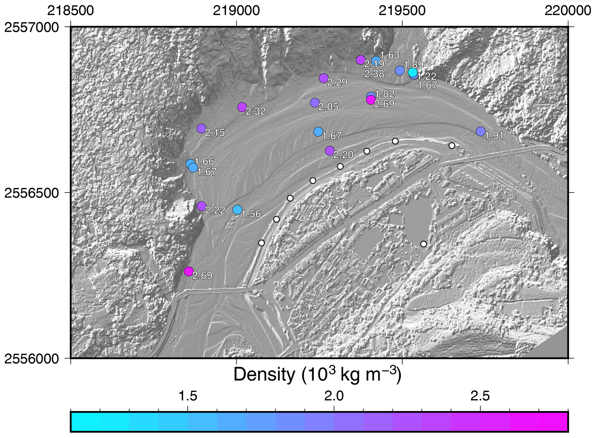
Figure 8 In situ density measured during the 2017 survey (colored dots; the value is also reported in white). Gravity sites are shown with white dots. Axes are in meters. The background is the shaded topography measured during the 2017 survey.

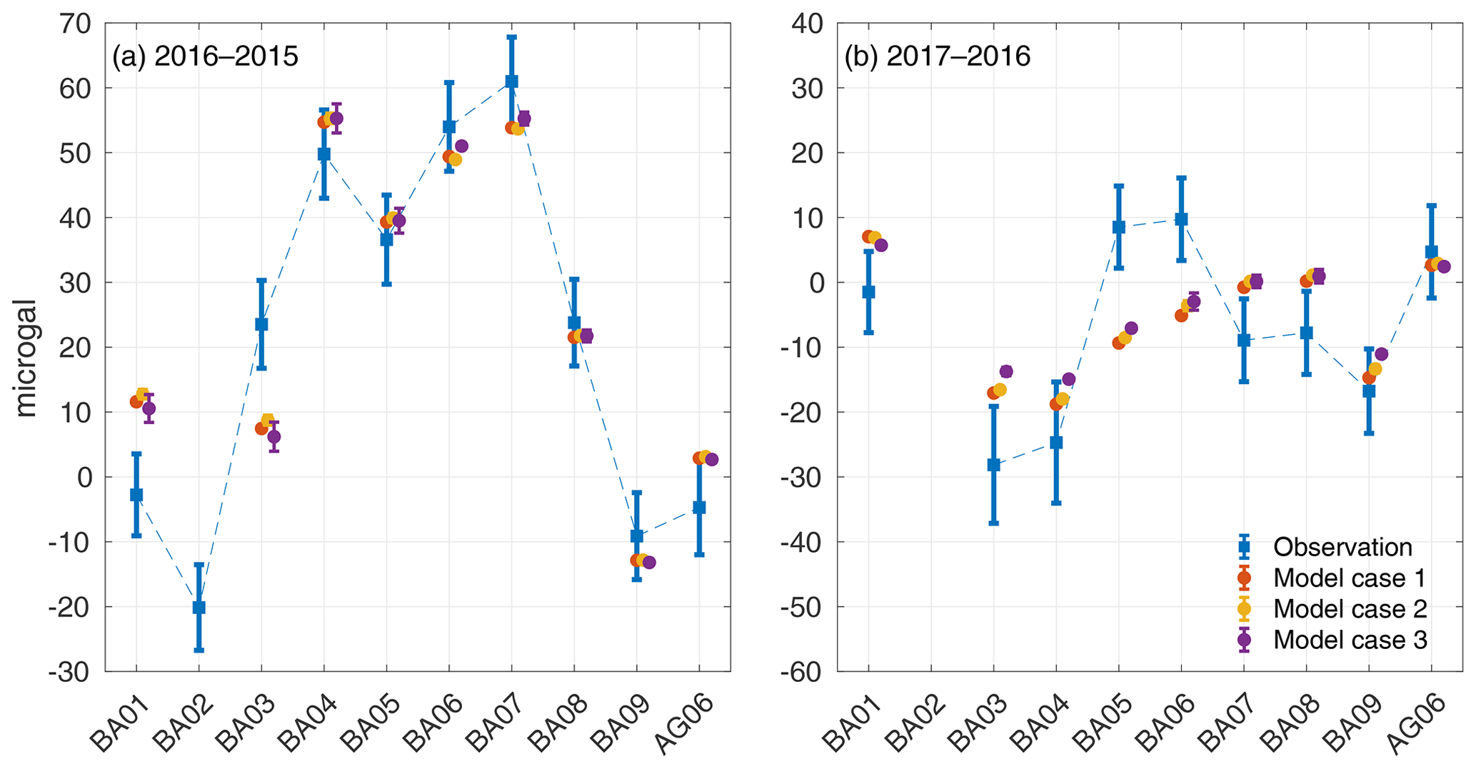
Figure 9 Comparison of the observed (blue) and modeled gravity changes for the densities inverted in cases 1, 2 and 3 (red, yellow and purple, respectively). Each case is slightly offset horizontally for legibility. No gravity is estimated at BA02 since its location is unknown.

The final comparison of the measured gravity and the computed gravity in cases 1, 2 and 3 is given in Fig. 9. The largest misfits are at BA05 and BA06 during the 2016–2017 period, for which gravity changes are underestimated by 19 and 15 µGal, respectively. Possible explanations for these two misfits are as follows: an incorrect site location, an error in the gravity data, an error in the DSM data and local but large hydrological effects not accessible at the scale of the global hydrological models we used. However, we could not narrow our search down to a specific issue at BA05 and BA06. At the other sites, the pattern and amplitude of the gravity observations are rather well explained by the modeling. Note that in Fig. 9b, the gravity modeled at most sites seems to need a small offset of −3 µGals to fit within the uncertainty of the observations. This may show that our absolute gravity estimate for the 2017 survey (Fig. 3) is wrong by 3 µGals.

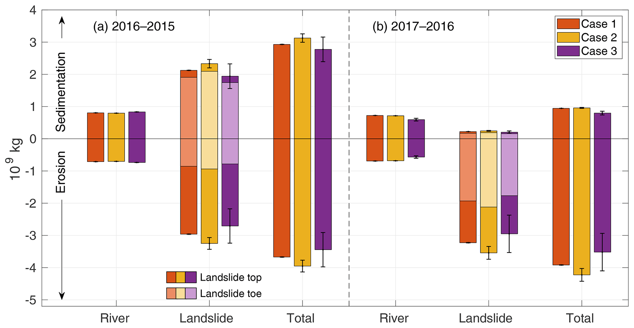
Figure 10 Estimation of the mass of sediment redistributed between 2016 and 2015 and between 2017 and 2016 in cases 1, 2 and 3 (red, yellow and purple, respectively; same color code as in Fig. 9). The mass estimation is shown for the river, the landslide and their sum (total). The error bars are computed by multiplying the volume variations from the DSM with the density uncertainties (Table 6). The landslide volumes distinguish the top and the toe of the landslides with a stacked bar plot form.

Multiplying the inverted densities (Table 6) with the volume changes computed from the DSM changes, we can eventually compute the mass of sediment that was redistributed between two surveys for each inversion case (Fig. 10). Since the inverted densities are similar in each case (Table 6) and the volume changes estimated from photogrammetry are identical, the estimated masses (volume times density) are also similar in each of the three cases. The difference mostly lies within the uncertainty of these estimates. In our mass estimation, we also differentiate the top and the toe of the landslide because the top of the landslide mostly experiences erosion while its toe undergoes both erosion and sedimentation. This helps to unravel how the sedimentation and erosion processes are distributed over the slow landslide.

In the river only, we observe that the mass of sediment redistributed between each survey is similar. The river gained between 0.61 and 0.83 × 10⁹ kg and lost between 0.58 and 0.74 × 10⁹ kg. Thus, the mass loss is about 4 % and 12 % less than the mass gain, resulting in a quasi-balanced budget that is within the uncertainty of the mass estimations. The time variability of the sediment mass budget is dominated by the landslide, which causes larger mass redistributions (up to 4 × 10⁹ kg) and loss-to-gain ratios. A significant mass loss occurred between 2016 and 2017, which is ∼ 15 times larger than the mass gain. Between 2015 and 2016, both erosion and sedimentation are significant at about 2 to 3 × 10⁹ kg and are rather balanced. A likely hypothesis is that we mainly observe a transfer of sediment from the top of the landslide, where 2.1 ± 0.4 × 10⁹ kg of material was eroded, toward its toe, where 1.9 ± 0.4 × 10⁹ kg accumulated (average mass from the three cases). Overall, from 2015 to 2017, the area lost about 3.7 ± 0.4 × 10⁹ kg of sediment. Note that this landslide occurs over several years and not in one quick event, probably as the consequence of the erosion by the meandering Laonong River.

6 Discussion

6.1 Implications for sediment transfers in active landscapes

Our results highlight how landscapes react to landsliding and how they evolve after a large perturbation such as Typhoon Morakot in 2009. Between 2015 and 2016, the activity of the Paolai slow landslide mostly consists of transferring about 2 × 10⁹ kg (about 1 × 10⁶ m³) of material from the landslide top to the landslide toe over roughly 100 to 200 m. After 2016, a significant event of erosion of the landslide occurs, with more than 3 × 10⁹ kg of sediment removed, including most of the sediment previously deposited on the landslide toe. This corresponds to a particularly rapid evacuation of the sediment, especially in the alluvial context of the Laonong River, which is consistent with predictions obtained with a morphodynamic model by Croissant et al. (2017) for bedrock rivers. It is likely that the position of the landslide in the outer bank of a meander has favored sediment export efficiency. Despite this landslide activity, it is quite remarkable that the Laonong River roughly maintains a neutral sediment budget over 2 years between 2015 and 2017 in the vicinity of the landslide. This means that the river mainly acts as a sediment transfer zone and that river incision and sediment evacuation occurring along the river is balanced by the sediment delivery occurring through the supply of landslide materials. This sediment supply may originate from the several large landslides triggered in the Paolai area by Typhoon Morakot in 2009 (Lin et al., 2011) and the following massive sediment aggradation along fluvial valleys up to 10, 30 and even possibly 100 m (DeLisle and Yanites, 2018; Hsieh and Capart, 2013). Our results would thus suggest that the Laonong River has not yet recovered from this aggradation phase and that the landscape is still perturbed by the aftermath of Typhoon Morakot even 8 years after its occurrence. This exceeds the relaxation time of 6 years observed after the 1999 Chi-Chi earthquake using river suspended load (Hovius et al., 2011) but is consistent with longer evacuation timescales of coarser, non-suspended materials (Yanites et al., 2010). Typhoon-triggered landslides occur every year in Taiwan, and global warming may intensify this process (Chiang and Chang, 2011). This could also build and maintain long-term sediment sources within the Taiwan range, which will keep supplying sediment into rivers even long after the Typhoon-Morakot-induced sources have been completely flushed.

6.2 Perspectives from recent advances in gravimetry

In this study we take advantage of the intense surface processes occurring in Taiwan to jointly analyze both time-variable gravity and photogrammetry measurements. Indeed, the amplitude of the sediment mass redistribution guarantees that we were able to measure significant gravity changes and, most importantly, surface elevation changes. Nevertheless, for rivers experiencing large and dynamic sediment mass redistributions that remain hidden beneath the water level, photogrammetric data would not bring any constraint on the density inversion. One would thus only be able to rely on the gravity measurements, leading to a nonuniqueness problem since both the density and the location of the redistributed sediment would have to be inverted. To better deal with this issue, we suggest two improvements to our gravity survey:

1. set a denser network of gravity sites, ideally with a mesh structure (more measurements, evenly distributed, meaning more constraints on the density inversion);

2. set this network closer to the mass changes to increase the gravity signal.

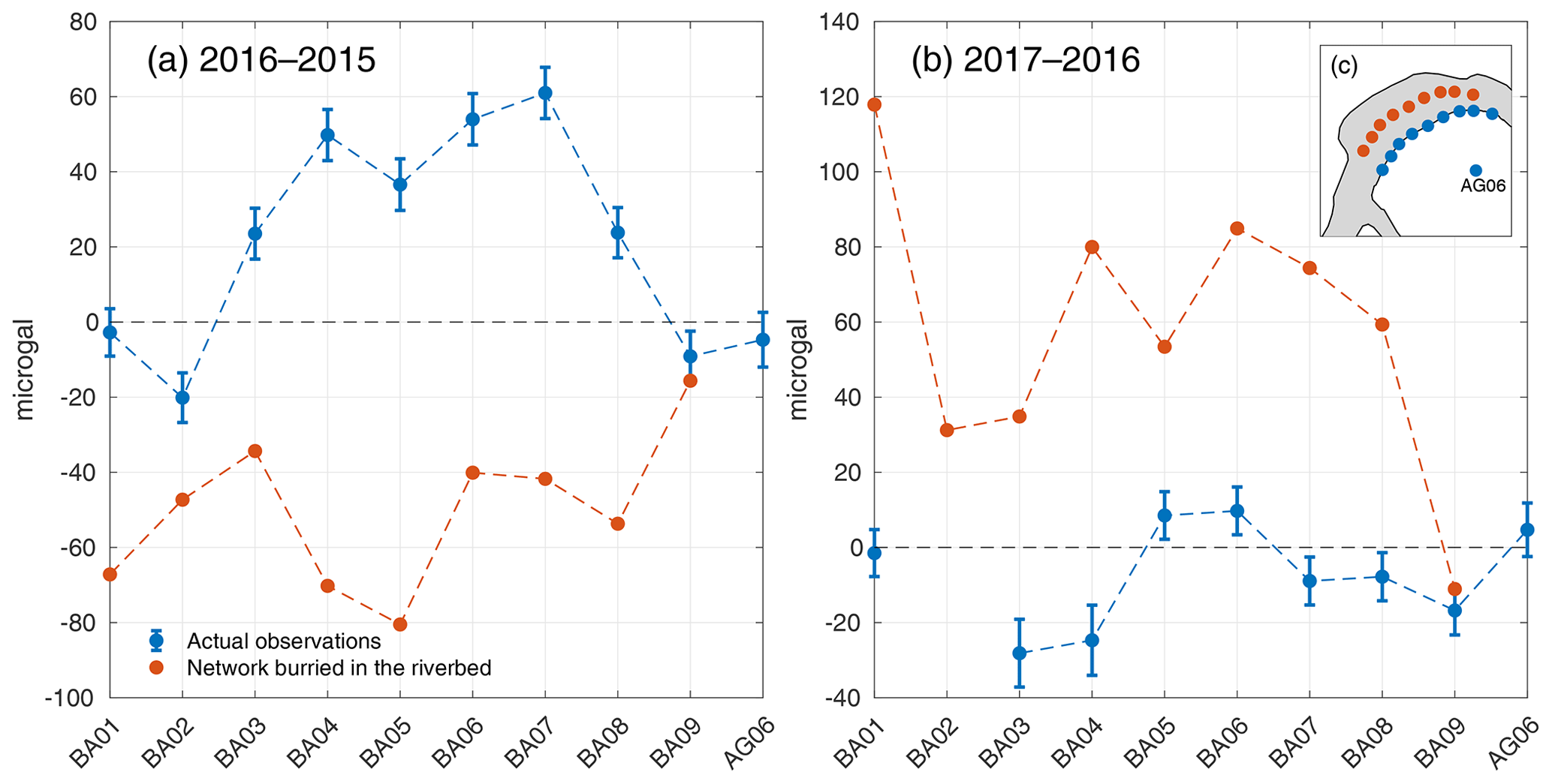
Figure 11 Gravity changes expected at new sites located 5 m beneath the river (red), compared with those measured at BA01–BA09 (blue), for the same sediment mass redistributions as (a) between 2015 and 2016 and (b) between 2016 and 2017. The new sites are in fact BA01–BA09 translated 140 m in the northeast direction, as illustrated in (c).

The best option would be to locate the gravimeters directly beneath the river bottom. Figure 11 shows that for such gravimeters, the average gravity change would increase from 31 to 50 µGal between 2016 and 2015 and from 13 to 61 µGal between 2017 and 2016.

This suggested survey design implies that gravimeters are set permanently over the time period of the project as they would not be easily accessible. Such a setup of permanent, buried gravimeters is presently impossible to realize with a CG-5 or any other contemporary relative or absolute gravimeter, but it remains realistic at a timescale of a few years. Indeed, a new generation of relative gravimeters is arriving from the use of microelectromechanical system (MEMS) technology, characterized by a significantly smaller size and lower price (Liu and Pike, 2016; Middlemiss et al., 2016, 2017). These shoebox-sized devices could be used to set permanent and dense gravity networks in rivers. However, setting persistent gravity networks in areas experiencing vigorous sediment transport will require deeper practical thinking. Gravity changes densely sampled over the river will make it possible to retrieve the sediment mass redistribution using gravity inversion methods (e.g., Camacho et al., 2011) further constrained by the geometry of the river and the depth of the relative gravimeter. In addition, as relative gravimeters suffer from instrumental drift, this permanent, buried network should be run in parallel either with permanent absolute measurements, which have recently become possible thanks to quantum gravimeters achieving 1 µGal repeatability (Ménoret et al., 2018), or with slowly drifting superconducting gravimeters (Hinderer et al., 2015). Therefore, ongoing progress in the development of terrestrial gravimeters may open new opportunities for quantifying the mass of sediment redistributed by surface processes. Another interest for having such a permanent gravity network is to monitor the dynamics of the sediment mass redistribution at timescales shorter than 1 year since the sediment concentration in Laonong River varies across the year (Fig. 12a).

Figure 12 (a) River level and sediment concentration of Laonong River, measured at Liugui station about 20 km downstream from Paolai. The highest sediment concentration (5000 ppm) was reached in summer 2017, when the river level increased by about 1.6 m. Data are freely available from the Taiwan WRA (Taiwan Water Resources Agency, 2019). (b) Estimated gravity changes at the buried network (Fig. 11c) as a function of the variations of the suspended sediment load and of increasing amounts of bed-load-transported sediment. The bed load fraction is considered here a homogenous layer of 0 to 60 cm thickness (labeled on each curve) and density 2 × 10³ kg m⁻³. The river becomes a debris flow when its suspended sediment concentration goes beyond 4 × 10⁴ ppm. The 5000 ppm level is shown as a reference. Note that the gravity sign is negative because the mass is increased above the gravimeters.

6.3 Continuous sediment transport estimation

The method and perspectives introduced so far aim at quantifying the mass of sediment redistributed by an event with a large sediment transport ability, such as a landslide or a high river discharge. The time step of this quantification depends on how long these events take to redistribute the sediment in a way that significantly alters the gravity measured at each site by, for example, > 10 µGal as an indicative change. Nevertheless, the best solution is to set a permanent gravity network so that any rapid sediment mass redistribution can be recorded. Figure 12a shows that the largest sediment concentration recorded at Liugui station is 5000 ppm (mass fraction), when the river level increased by 1.6 m.

For the hypothetical permanent, buried gravity network (Fig. 11c), we compute the gravity effect of a river level change of 1.6 m, which covers the entire area of the active bed channel of the Laonong River. The 5000 ppm sediment concentration means there is 5 kg of sediment in 1000 kg of river fluid and hence 995 kg of pure water. In this framework, and assuming that the density of the sediment is 2 × 10³ kg m⁻³, we can compute the density change due to rising sediment concentrations up to 10⁶ ppm, meaning the river is made of sediment only. The gravity variation solely due to a shift from 0 to 5000 ppm of suspended sediment is about 0.17 µGal on average over each site. This cannot be properly distinguished from the main gravity change due to the rising river water level. In fact, the suspended sediment concentration would need to increase by about 3 × 10⁵ ppm to change the gravity by at least 10 µGal (Fig. 12b with the bed load set to 0 cm). This corresponds to a concentrated debris flow nearly 8 times more concentrated than the threshold of 4 × 10⁴ ppm used for the definition of a debris flow (Dadson et al., 2005; Lin and Chen, 2013). However, sediment is also transported on the riverbed, as bed load, and its variation must be added to the variation of suspended sediment concentration to estimate the effect of sediment discharge variations on gravity. We have no measurement of this bed load component for Laonong River, but measurements in another catchment of Taiwan showed that 50 % of the cumulative mass of the bed load was built by rocks with a diameter less than 15 cm (D₅₀=15 cm) and that 90 % of the cumulative mass was built by rocks with a diameter less than 62.5 cm (D₉₀=62.5 cm) (Cook et al., 2013). Therefore, we compute the effect of adding homogenous bed load layers of up to 60 cm thickness and density 2 × 10³ kg m⁻³ to suspended sediment variations (labeled curves in Fig. 12b). This addition generates about 50 µGal of gravity variation, which would be clearly identifiable in the gravity measurements. This computation gives an order of magnitude of the gravity change expected from time-varying suspended and bed load transport. It shows that continuous time-variable gravity could quantify changes in sediment discharge if the sediment concentration rises by at least 3 × 10⁵ ppm without bed load or if the bed load increases to a thickness of at least 12.5 cm, under the assumption that only gravity changes above 10 µGal are significant. More accurate predictions of gravity effects require knowing the proportionality relation, if any, between the suspended and bed load component, as well as local hydrogravity models. Again, this 10 µGal threshold is linked to the accuracy of the gravimeter, but ongoing advances and interest in time-variable gravimetry may fuel the development of devices with higher accuracies.

7 Conclusions

This study shows that the mass of sediment redistributed by rivers and landslides can be estimated by combining time-lapse gravimetric and photogrammetric measurements. Focusing on the Laonong River in southern Taiwan, we estimate that about 3.7 ± 0.4 × 10⁹ kg of sediment was removed from 2015 to 2017 around our study site. This sediment loss is mainly due to a slow landslide moving from one year to another. The sediment budget (i.e., the difference between sedimentation and erosion) within the river is close to zero, although more surveys should be carried out to identify longer-term deposition or erosion in this area. The average sediment density obtained with this method (1.9 ± 0.01 × 10³ kg m⁻³) is similar to the average sediment density measured in situ across the flood plain (2.0 × 10³ kg m⁻³). The new method introduced in this paper has the advantage of being able to directly sense the mass of sediment and can benefit many studies on surface processes, which require quantitative estimates of sediment mass redistribution. Although time-variable gravimetry remains a rather expensive method with demanding survey constraints, it has undergone promising progress in recent years. One is the significant miniaturization of the devices using inexpensive MEMS technology (Middlemiss et al., 2016) and the other is the realization of permanent absolute gravimeters using cold atom interferometry (Ménoret et al., 2018). Such new tools could be further used without photogrammetry for rivers where most of the sediment transport is hidden under the water. If the suspended and bed load transports are significant enough, measuring the instantaneous sediment discharge could also become a reasonable project.

Appendix A: Processing of the relative gravity survey

Figures A1–A3 summarize how each relative survey was done in 2015, 2016 and 2017, respectively. All relative loops start and end at AG06, and other relative gravity sites (prefix BA) are remeasured several times for each survey within a few hours. It is necessary to have such repeated measurements in order to estimate and remove the instrumental drift of the CG-5 relative gravimeter. The adjustment is done using the software Gravnet (Hwang et al., 2002), assuming that drift is linear with time. The instrumental drift for each year are as follows:

• 2015: 0.032 ± 0.037 mGal d⁻¹;

• 2016: −0.085 ± 0.004 mGal d⁻¹;

• 2017: −0.161 ± 0.007 mGal d⁻¹.

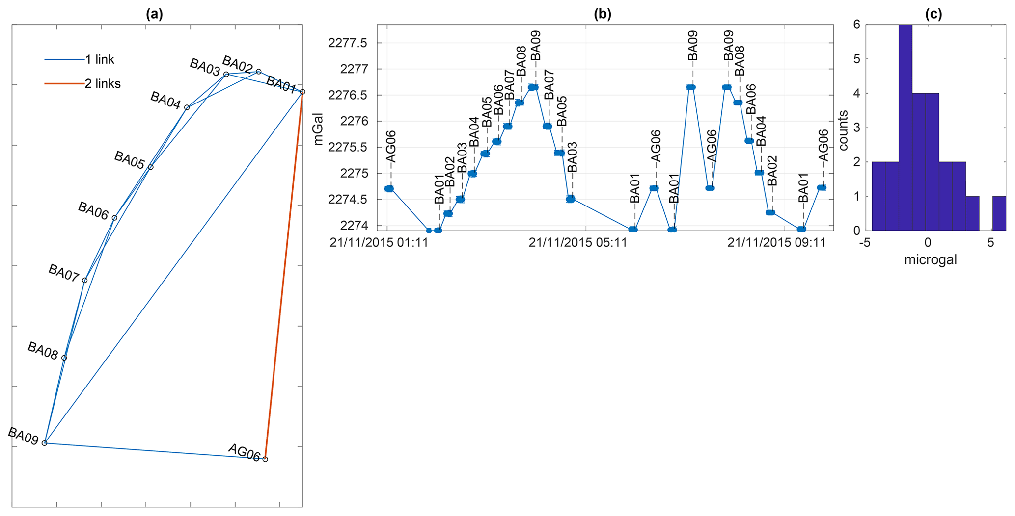
Figure A1 (a) Map view of the relative gravity network with the link between each site for the 2015 survey. (b) Gravity readings on the CG-5 at each site as a function of time. (c) Histogram of the residuals after the drift adjustment.

Figure A2 (a) Map view of the relative gravity network with the link between each site for the 2016 survey. (b, c) Gravity readings on the CG-5 at each site as a function of time. (d) Histogram of the residuals after the drift adjustment.

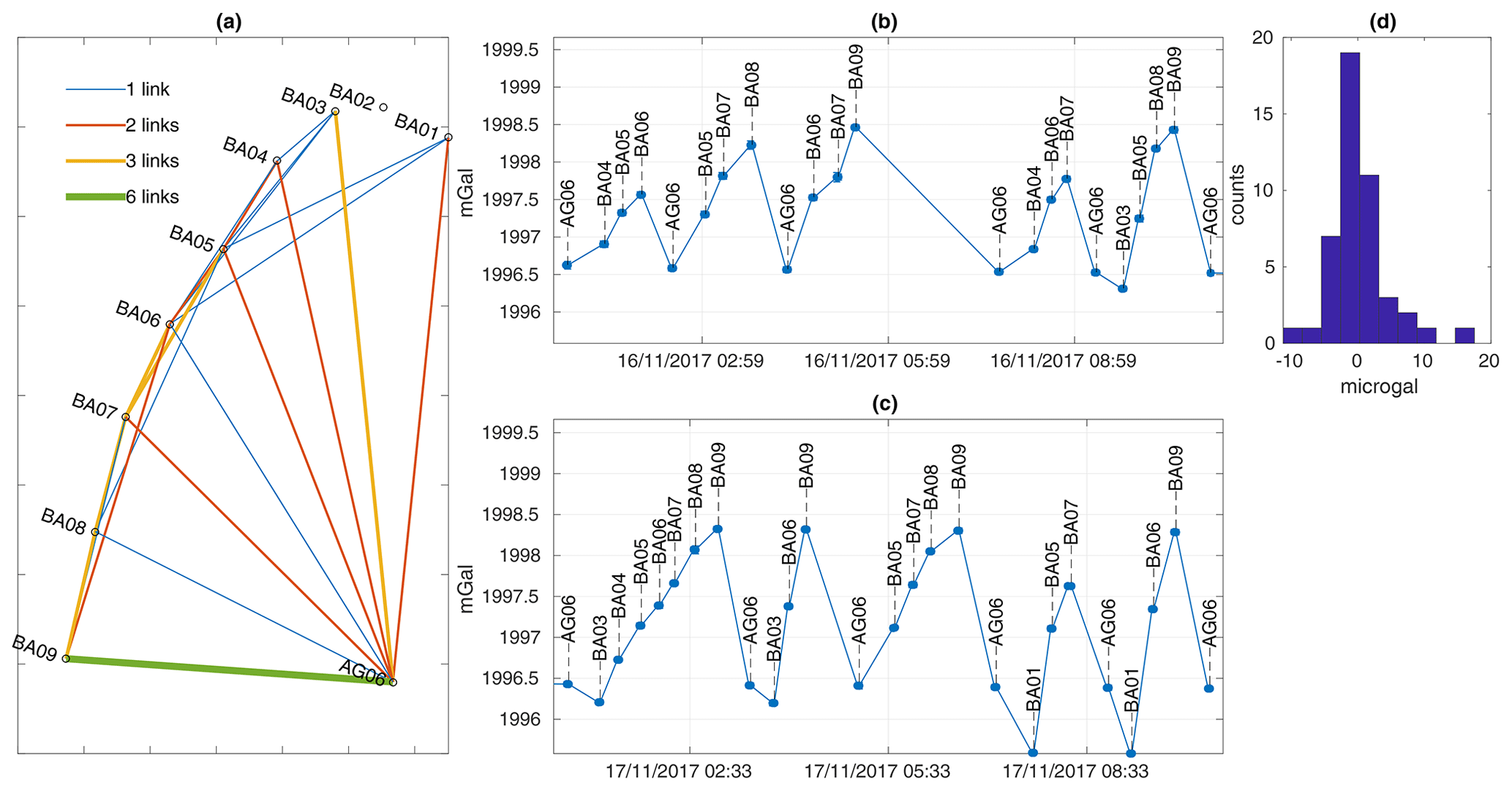
Figure A3 (a) Map view of the relative gravity network with the link between each site for the 2017 survey. (b, c) Gravity readings on the CG-5 at each site as a function of time. (d) Histogram of the residuals after the drift adjustment.

Appendix B: Gravimetric effect of the dolosse

Figure B1a is a picture of the dolosse stacked near the gravity site BA02. The side L and height H are reported with blue lines for comparison with Fig. B1c and d. They are made of three identical patterns, which repeat around the center of the dolos and close it. The center of the dolos and part of its sides are empty. However, due to its limited spatial resolution, the photogrammetry “sees” the dolosse as plain hexagons (Fig. B1b). Our aim is thus to define the ratio k between an actual dolos and a plain dolos. This ratio is then multiplied by the average density ρ_c of concrete (2.3 × 10³ kg m⁻³), which the dolosse are made of. In this way we obtain an effective dolos density which we pair to the volume obtained from the photogrammetry and eventually use to compute the gravitational effect of the dolosse at our study sites.

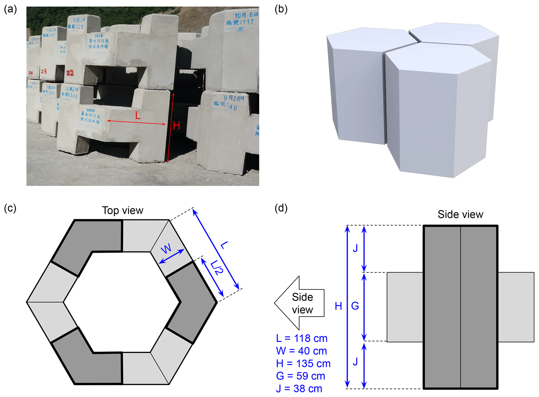
Figure B1 (a) Photograph of the dolosse. (b) 3-D hexagonal shape of the plain dolos as seen by the photogrammetry. (c) Top view of the actual dolos. The dark gray parts are the pillars actually touching the ground and the light gray parts are the “arms” of the dolos. (d) Side view of one dolos element. One dolos consists of three of these parts joined by the arms.

The volume Vp of a regular hexagon with side L and height H is

$$\begin{array}{}\text{(B1)}& V={\displaystyle \frac{\mathrm{3}}{\mathrm{2}}}\sqrt{\mathrm{3}}{L}^{\mathrm{2}}H=\mathrm{4.9}{\mathrm{m}}^{\mathrm{3}}.\end{array}$$

The volume Vd of the actual dolos is estimated at 1.6 m³, using the geometry detailed in Fig. B1c and d.

Therefore, we find that the true volume of the dolos is $k=\mathrm{1.6}/\mathrm{4.9}\cong \mathrm{0.33}$, which is one-third of the plain volume; hence its effective density is 2.3k=0.76 × 10³ kg m⁻³. The geometry and density of the dolosse were used to compute their gravitational attraction at BA04 and BA05 using gravity modeling by rectangular prism methods (Nagy, 1966). This effect is about −15 µGal.

Appendix C: In situ determination of the river material density

Site selection

We select 20 sites in the active river channel, which are accessible by walking. We try to find sites where materials are different, some of them being close to each other, to better grasp the variety of the material in the channel. Nevertheless, we also try to have a spatially even sampling. In a few places, two samplings are done at the same horizontal position but at the surface and then deeper. All site positions are recorded with a hand GPS (about 3 m accuracy).

Material sampling

At each start, we first distribute several benchmarked rules all around the place that will be sampled (Fig. C1a). Several pictures are taken to cover the sampling site and several benchmarked rules at a time. Pictures should overlap with each other. We then dig a hole of about 30–40 cm depth and radius, paying attention to not move any of the benchmarked rules. The excavated material M is put in a bucket of known mass and weighed using a hanging hook weight machine. Then another set of pictures is taken to cover again the benchmarked rules and the hole just dug. The only difference between the pictures taken before and after is the hole.

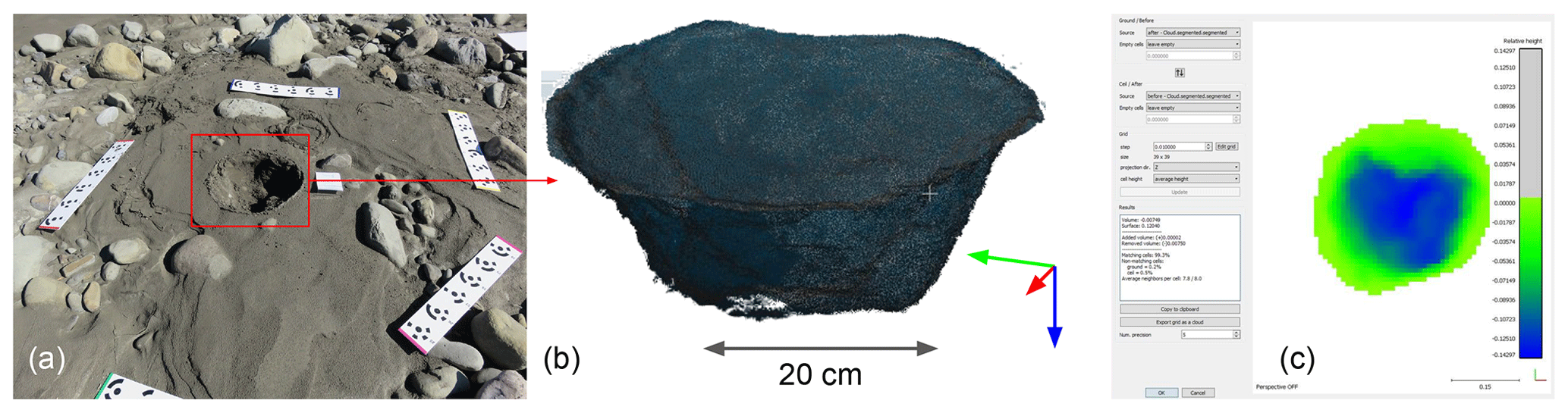
Figure C1 (a) Picture of the hole taken with references scales and benchmarks. Several pictures were thus taken before and after the hole was dug. (b) 3-D cloud of the points mapping the surface of the hole. (c) Computation of the volume bounded by the hole and the former surface of the ground before the hole was done.

Photogrammetry

The benchmarked rules make a common reference between the pictures taken before and after the hole is dug. They are transformed into clouds of points in 3-D (Fig. C1b), one representing the original surface, the other representing the dug surface. Thus, subtracting these two surfaces returns the surface of the hole, from which the volume V of the hole is computed (Fig. C1c).

Density computation

The density at the sampling site is then M divided by V.