Morphometric properties of alternate bars and water discharge: a laboratory investigation

The formation of alternate bars in straightened river reaches represents a fundamental process of river morphodynamics that has received great attention in the last decades. It is well-established that migrating alternate bars arise from an autogenic instability mechanism occurring when the channel width-to-depth ratio is sufficiently large. While several empirical and theoretical relations are available for predicting how bar height and length depend on the key dimensionless parameters, there is a lack of direct, quantitative information about the dependence of bar properties on flow discharge. We performed a series of experiments in a long, mobile-bed flume with fixed and straight banks at different discharges. The self-formed bed topography was surveyed, different metrics were analyzed to obtain quantitative information about bar height and shape, and results were interpreted in the light of existing theoretical models. The analysis reveals that the shape of alternate bars highly depends on their formative discharge, with remarkable variations in the harmonic composition and a strong decreasing trend of the skewness of the bed elevation. Similarly, the height of alternate bars clearly decreases with the water discharge, in quantitative agreement with theoretical predictions. However, the disappearance of bars when discharge exceeds a critical threshold is not as sharp as expected due to the formation of so-called “diagonal bars”. This work provides basic information for modeling and interpreting short-term morphological variations during individual flood events and long-term trajectories due to alterations of the hydrological regime.

1 Introduction

Alternate bars are large-scale bedforms characterized by a repetitive sequence of scour holes and depositional diagonal fronts with longitudinal spacing on the order of several channel widths, which are observed in both sand and gravel bed rivers (e.g., Engels, 1914; Jaeggi, 1984; Rhoads and Welford, 1991; Church and Rice, 2009; Jaballah et al., 2015; Rodrigues et al., 2015). They have been extensively studied in the last 50 years because of both their practical and theoretical relevance. From the point of view of river engineering, alternate bars are undesired for their erosional effect on banks and bridge piers and their depositional effect that can disturb navigation and increase flooding risk. From an ecosystem perspective, alternate bars represent one of the relevant morphological units creating suitable habitats for aquatic fauna and riparian vegetation, which contributes to ecological diversity (Gilvear et al., 2007; Zeng et al., 2015). Lastly, from a theoretical point of view, they represent a fascinating phenomenon, which plays a fundamental role in the dynamics of a variety of fluvial systems, such as meandering rivers, channel bifurcations, and braided rivers (e.g., Lewin, 1976; Parker, 1976; Fredsoe, 1978).

A number of studies (e.g., Hansen, 1967; Callander, 1969; Sukegawa, 1972; Parker, 1976; Fujita and Muramoto, 1982; Nelson, 1990) have demonstrated that downstream-migrating alternate bars spontaneously develop in straight, channelized reaches as the result of the instability of a cohesionless bed. Due to this autogenic formation mechanism, this kind of bed morphology is often referred to as “free bars” (Seminara and Tubino, 1989). More specifically, theoretical and laboratory experiments (Fredsoe, 1978; Jaeggi, 1984; Fujita and Muramoto, 1985; Colombini et al., 1987; Lanzoni, 2000a) identified the channel width-to-depth ratio as the key controlling parameter for the formation of free alternate bars: when the channel is relatively narrow, the effect of gravitational pull on the bed load transport is relatively strong and tends to suppress any transverse bed gradient; conversely, in relatively wide channels, initially small, periodic perturbations of the bed elevation generate a topographic steering of the flow field that in turn produces a growth of the bed perturbation itself, which leads to the spontaneous, self-sustained development of alternate bars. Therefore, it is possible to define a threshold value of the aspect ratio (i.e., the half-width-to-depth ratio), β_cr, representing the lower limit at which alternate bars are expected to form.

However, when the width-to-depth ratio is smaller than the threshold value, the equilibrium bed configuration is not necessarily planar, as other bed features may result from different instability mechanisms, such as short, shallow, and fast-migrating three-dimensional bedforms, usually called diagonal bars (Einstein and Shen, 1964; Jaeggi, 1984; Colombini and Stocchino, 2012). Since the transition between alternate and diagonal bars is not always sharp and since they are both characterized by a diagonal pattern, they can be easily confused. Nonetheless, as highlighted by Colombini and Stocchino (2012), diagonal bars represent a clearly distinct kind of bedform and should be regarded as three-dimensional oblique dunes. In fact, they are the product of different formation mechanisms (e.g., they cannot be described by shallow-water two-dimensional models), and they depend on different controlling parameters (water depth and Froude number). Conversely, when the aspect ratio becomes very large, transition to more complex, wandering, and braiding multi-thread channels is observed (e.g., Parker, 1976; Fredsoe, 1978; Eaton et al., 2010; Ahmari and Da Silva, 2011; Garcia Lugo et al., 2015), which poses an upper limit to the range of β values within which free alternate bars are expected to form.

Under steady flow conditions, free bars attain an equilibrium state, whereby they migrate downstream without changing their morphology (Ikeda, 1984; Colombini et al., 1987). Several theoretical and empirical relations for estimating the equilibrium bar height and wavelength are available (e.g., Ikeda, 1984). Specifically, weakly nonlinear theories (Colombini et al., 1987; Bertagni and Camporeale, 2018) allow for a physically based, analytical prediction of how the equilibrium bar configuration depends on the dimensionless channel and flow parameters.

Nevertheless, there is basically no direct, quantitative analysis regarding how equilibrium properties of alternate bars depend on water discharge. In particular, very few data exist about the shape of alternate bars, as previous experiments have mainly focused on bar height, wavelength, and growth rate (e.g., Ikeda, 1984; Jaeggi, 1984; Fujita and Muramoto, 1985; Lanzoni, 2000a). Moreover, there is little knowledge about the transition from alternate bars to plane-bed or diagonal bar configurations, which may occur when varying the flow discharge. This lack of information makes it difficult to understand how changes in the flow regime may alter bed morphology. In this work we follow an integrated experimental and theoretical approach to address the following research questions. (i) How do geometrical properties of alternate bars depend on water discharge? (ii) Is it possible to identify different bar styles depending on flow conditions? (iii) Is there a sharp transition from alternate bar morphology to a plane-bed configuration? To answer these questions a series of experiments was performed in a flume with identical channel conditions and sediment characteristics but differing flow discharge, and experimental results were compared with theoretical predictions from the weakly nonlinear model of Colombini et al. (1987).

2 Methods

2.1 Laboratory setup

Laboratory experiments were conducted in a 24 m long flume at the Hydraulics Lab of the University of Trento. The physical model consisted of a straight channel of width W=0.305 m, with vertical banks built out of plywood covered by a thick plastic tarp. Uniform sand with a median diameter of d₅₀=1.01 mm was used as feed and bed material. Discharge and sediment input to the flume was set automatically using a recirculating pump and a calibrated screw feeder. At the downstream end of the flume, the output bed load accumulated in a large filtering crate, which was weighted every 10 s by means of four load cells. A laser profiler moving on high-precision rails mapped the topography of the drained bed with a vertical accuracy of 0.1 mm and spatial resolution of 50×5 mm (longitudinal and transverse direction, respectively). A set of 16 steady flow runs were performed, with discharge ranging from Q=0.5 to 4.2 L s⁻¹; all but two of the discharge values (1.5 and 4.2 L s⁻¹) were repeated twice to obtain a larger dataset of bed topographies. The chosen discharge values ensure a wide range of channel aspect ratios and are associated with the hydraulic conditions reported in Table 1. At the beginning of each model run, the bed was graded to a slope S=0.01 using a blade mounted on a movable trolley. Sediment supply for each run was first assigned on the basis of previous experiments carried out with a similar setup (Garcia Lugo et al., 2015) and gradually adjusted during the transient phase of the run to match bed load output. The duration of experimental runs was chosen to ensure equilibrium conditions, which amounts to 10–20 times the Exner timescale (see Garcia Lugo et al., 2015). Wetted width (W_w) and active width (W_a) were measured at 20 regularly spaced cross sections twice per run and averaged in space and time. The migration rate of the alternate bars was estimated by tracking the position of up to 15 individual bar fronts at fixed time intervals. At the end of each run the bed was drained to acquire topography data. Laser surveys covered a 20.5 m long area starting 2 m downstream of the inlet to exclude the effect of local disturbances. The average sediment flux, Q_s, was estimated on the basis of the total weight of the transported material, excluding the first transitory part of the experiment (an equilibrium condition was considered achieved when the cumulative mean of the bed load signal fell within 5 % of the global mean).

Table 1 Summary data from the laboratory experiments. Channel width, slope, and median grain size are constant and equal to W=0.305 m, S=1.0 %, and d₅₀=1.01 mm, respectively. The Rouse number is defined as $\mathit{\text{Ro}}=w_{\mathrm{s}}/\left(\mathit{\kappa }{u}_{\ast }\right)$, where κ=0.4 is the von Kármán constant, u_∗ is the friction velocity, and w_s is the settling velocity of the bed particles computed according to Ferguson and Church (2004). The water depth, Froude number, Shields number, Rouse number, and aspect ratio are computed by assuming uniform flow conditions over a plane bed and considering the friction formula in Eq. (9).

2.2 Topography data processing

Laser surveys were processed by removing points falling outside the channel bed and by subtracting the average longitudinal slope. This allowed for obtaining digital elevation models (DEMs) of the detrended bed elevation. The investigation of the geometric properties of alternate bars required the identification of individual bar units. To this aim, we applied the widely accepted definition of bar wavelength as the length between two successive troughs (Eekhout et al., 2013) and developed an automatic procedure to map the position of troughs on DEMs. Elevation maps of individual bars were obtained by splitting DEMs at trough points. Bars that were very irregular or only partially within the study area were excluded from further calculations. Bar DEMs were normalized by subtracting the elevation mean.

To facilitate the comparison of the shape of individual bars, spatial coordinates of each bar DEM (x,y; see Fig. 1a) were scaled by the bar wavelength (L) and the channel width (W), which resulted in stretched DEMs with both coordinates ranging from 0 to 1. Individual DEMs were then resampled using an inverse distance-weighted routine to obtain elevation data on the same regular grid of 64×64 points. An ensemble bar was defined as the mean elevation of each grid point across the bars formed at the same discharge, thus representing a characteristic average bar shape that can be used to study the effect of different experimental conditions.

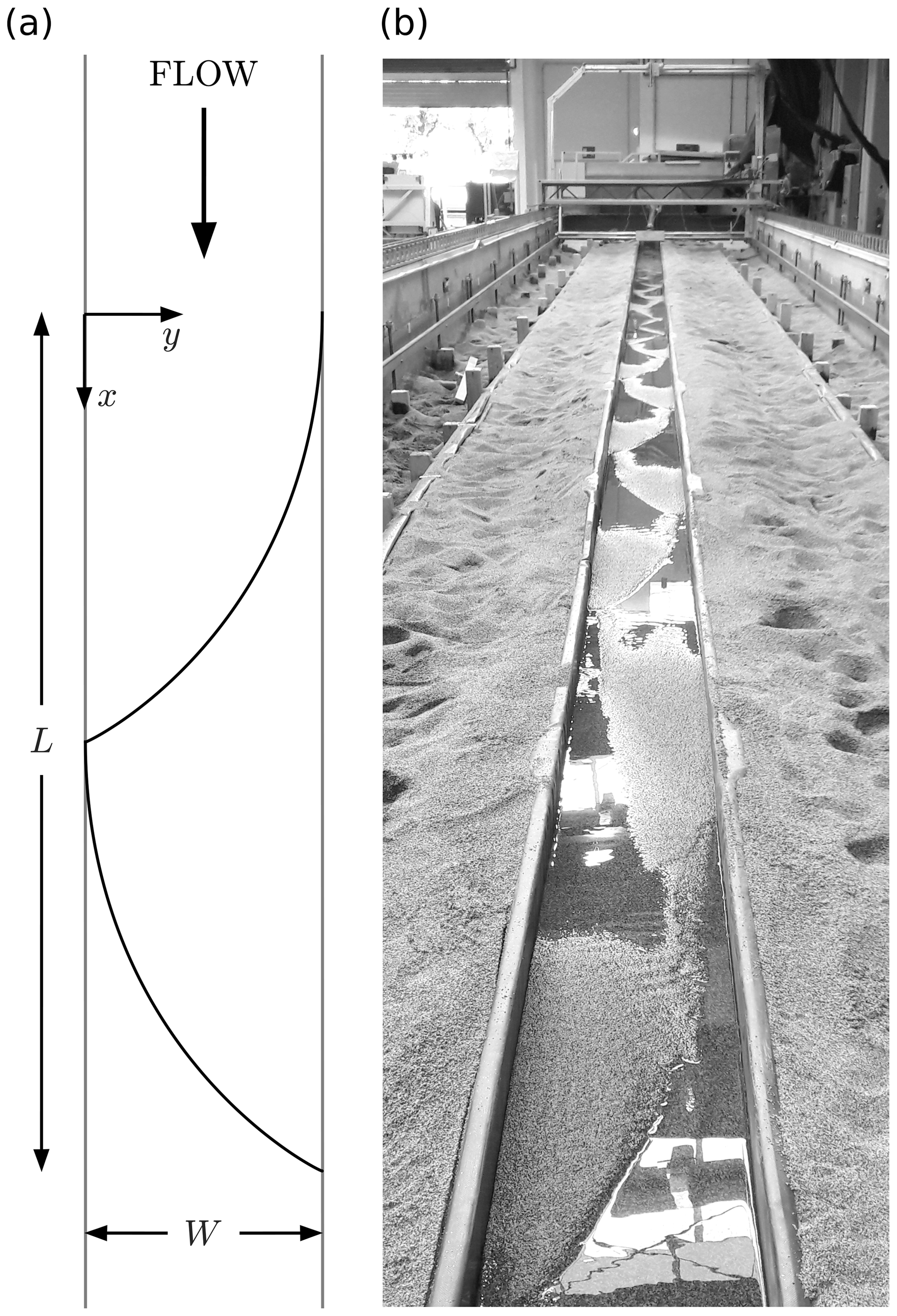
Figure 1 (a) Reference system (x,y) for an individual bar of wavelength L in a straight channel of width W, with the curved line indicating the typical position of bar fronts. (b) Picture of the flume at the end of the experiment with $Q=\mathrm{2.5}\mathrm{L}{\mathrm{s}}^{-\mathrm{1}}$, showing the presence of alternate bars. Flow is from top to bottom.

2.3 Different metrics to characterize bar properties

Alternate bars are commonly described in terms of their wavelength, height, and migration rate. Bar wavelength is the distance between consecutive, corresponding points along the flow direction. Bar height is usually defined as the vertical distance between the bottom of the pool and the top of the bar surface, with several method and metrics proposed in the literature. Finally, for freely migrating bars, the migration rate is the speed at which the bar front moves downstream. However, the geometrical properties of bars are not limited to their height and wavelength, as more detailed information about their geometrical shape can be derived by analyzing the bed morphology.

2.3.1 Metrics for bar height and bed relief

The most intuitive and widely used way to define bar height is the difference between the maximum and minimum elevation within a bar unit, computed after removing the mean bed slope. Though different symbols have been used in the literature, we refer to the Ikeda (1984) notation, namely

$$\begin{array}{}\text{(1)}& H_{\mathrm{BM}}=max\left(\mathit{\eta }\right)-min\left(\mathit{\eta }\right),\end{array}$$

where η indicates the (detrended) bed elevation. A slightly different definition of bar height (e.g., Fujita and Muramoto, 1985) is based on computing the elevation difference along individual transverse cross sections (H_Bsec) and then taking its maximum value (H_B):

$$\begin{array}{}\text{(2)}& \begin{array}{rl}& H_{\mathrm{Bsec}}={\max }_{\sec }\left(\mathit{\eta }\right)-{\min }_{\sec }\left(\mathit{\eta }\right),\\ & H_{\mathrm{B}}=max\left(H_{\mathrm{Bsec}}\right),\end{array}\end{array}$$

where max_sec and min_sec denote the maximum and minimum elevation along individual cross sections.

The above definitions have a clear physical meaning, as they directly represent the bar height from the crest to the trough. However, being based on extreme elevation values, such metrics are sensitive to outliers and measurement errors. Therefore, it is sometimes convenient to estimate the topographic effect of alternate bars through different metrics, which measure the “relief” rather than the bar height. Specifically, the bed relief can be defined through the standard deviation of the elevation distribution,

$$\begin{array}{}\text{(3)}& \mathrm{SD}=\mathrm{SD}\left(\mathit{\eta }\right),\end{array}$$

or, alternatively, through the bed relief index (e.g., Hoey and Sutherland, 1991; Liébault et al., 2013), which is defined on a cross-sectional basis as follows:

$$\begin{array}{}\text{(4)}& \begin{array}{rl}& {\mathrm{BRI}}_{\sec }={\mathrm{SD}}_{\sec }\left(\mathit{\eta }\right),\\ & \mathrm{BRI}=\mathrm{mean}\left({\mathrm{BRI}}_{\sec }\right),\end{array}\end{array}$$

where SD_sec indicates the standard deviation calculated along individual cross sections.

All of these metrics are first computed for each individual bar and then averaged among all bars formed at the same discharge. It is important to note that, while H_BM and SD are based on the full 2-D distribution of elevation, H_B and BRI are based on the elevation along individual cross sections. Since the highest and lowest points of a bar do not necessarily occur along the same cross section, H_B and BRI are expected to provide a lower estimate of height if compared to H_BM and SD, respectively.

2.3.2 Metrics for the bar shape

One method to characterize the shape of bars is via the skewness parameter (SK), which measures the asymmetry of the bed elevation distribution, thus providing information on the relative proportion of high and low areas within a bar. Riverbed elevation maps often show negative skewness, with deep, narrow channels carved into large, higher-elevation bars (e.g., Bertoldi et al., 2011; Garcia Lugo et al., 2015).

Being based on the relative frequency of the elevation values, the above metrics, however, do not to provide information about the spatial arrangement of the bedforms. To obtain synthetic information about the spatial structure of bars, we analyzed the bed elevation maps through the two-dimensional Fourier transform (e.g., Garcia and Nino, 1994; Zolezzi et al., 2005). As detailed in Appendix A, the topography of an individual bar of wavelength L (see Fig. 1a) can be represented as follows:

$$\begin{array}{}\text{(5)}& \begin{array}{rl}\mathit{\eta }(x,y)& =\sum _{m=\mathrm{0}}^{\mathrm{\infty }}\sum _{n=\mathrm{0}}^{\mathrm{\infty }}\left|A_{nm}\right|\cos (\mathit{\pi }my/W)\\ & \cos \left(\mathrm{2}\mathit{\pi }nx/L+{\mathit{\varphi }}_{nm}\right),\end{array}\end{array}$$

where x is the longitudinal coordinate, y is the transverse coordinate (with origin at the right bank), and $\left|A_{nm}\right|$ and ϕ_nm represent the amplitude and phase of each Fourier component. The amplitudes of the main components provide information about possible symmetry properties, the relative importance of two-dimensional and three-dimensional topographic effects, and the deviation from the simple sinusoidal structure that arises from linear stability analyses (e.g., Fredsoe, 1978).

2.4 Application of the weakly nonlinear theory of Colombini et al. (1987)

The theory of Colombini et al. (1987) is based on a weakly nonlinear solution of the two-dimensional shallow-water and Exner model for a straight channel of constant width and downstream gradient. Specifically, they considered the following relation for the bed load transport rate per unit width, q_b (m² s⁻¹):

$$\begin{array}{}\text{(6)}& q_{\mathrm{b}}=\sqrt{g\mathrm{\Delta }{d}_{\mathrm{50}}^{\mathrm{3}}}\mathrm{\Phi },\end{array}$$

where g is the gravitational acceleration, Δ=1.65 is the relative submerged weight of sediment, and Φ represents the dimensionless sediment transport, whose expression depends on the choice of the transport formula. Moreover, the effect of the lateral bed slope on the direction of the bed load transport was modeled according to the Ikeda (1982) formulation:

$$\begin{array}{}\text{(7)}& \tan \left(\mathit{\gamma }\right)=-{\displaystyle \frac{r}{\sqrt{\mathit{\theta }}}}{\displaystyle \frac{\mathrm{d}\mathit{\eta }}{\mathrm{d}y}},\end{array}$$

where γ is the angle between the velocity vector and the sediment transport vector, θ is the Shields number, and r is an empirical dimensionless parameter typically ranging from 0.3 to 0.6.

The model of Colombini et al. (1987) allows for different choices of the transport and friction formulas. For the present analysis, we considered the Parker (1978) relation, which gives the following expression for the dimensionless sediment transport:

$$\begin{array}{}\text{(8)}& \mathrm{\Phi }=\mathrm{11.2}{\mathit{\theta }}^{\mathrm{1.5}}{\left(\mathrm{1}-{\displaystyle \frac{{\mathit{\theta }}_{\mathrm{i}}}{\mathit{\theta }}}\right)}^{\mathrm{4.5}},{\mathit{\theta }}_{\mathrm{i}}=\mathrm{0.03},\end{array}$$

where θ_i indicates the Shields number of incipient sediment motion. This transport formula was chosen for two reasons: (i) it exhibits a critical threshold that is consistent with our experiments, and (ii) it is suitable for analytical treatment because for θ>θ_i it is continuous and has continuous derivatives. Moreover, as in the original formulation of Colombini et al. (1987), we used the logarithmic friction formula of Engelund and Fredsoe (1982), which gives the following expression for the dimensionless Chézy coefficient:

$$\begin{array}{}\text{(9)}& c=\mathrm{6}+\mathrm{2.5}\log \left({\displaystyle \frac{D}{\mathrm{2.5}{d}_{\mathrm{50}}}}\right),\end{array}$$

where D indicates the water depth. Finally, we calibrated the empirical parameter r of Eq. (7) by minimizing the difference between experimental and analytical values of H_BM, which resulted in a value of 0.40.

3 Results

The bed topographies obtained under different discharges are illustrated in Fig. 2. A regular pattern of large-scale bedforms can be recognized in all maps, with substantial differences in shape and relief. At the lowest discharge (0.5 L s⁻¹) the bed shows a complex topography with alternate, elongated pools along the banks but few clearly discernible bar fronts and several small channels cutting the main bedforms. In these conditions, the tops of bars (3 % of the area; see Table 1) begin to emerge and less than half of the bed surface is actively transporting sediments. At higher flows (1.0 and 1.5 L s⁻¹), bed topography is dominated by a coherent pattern of bars with elongated pools and a sharp front that is almost transverse to the flow direction. Between Q=2.0 and 2.7 L s⁻¹, relief progressively decreases and bar fronts become curved and oblique in a regular fish-scale pattern. Finally, between Q=3.0 and 4.2 L s⁻¹, bars are shorter and shallower. It is important to note that for increasing discharge, well-defined bars progressively disappear from the upstream end of the channel, where the bed shows a superimposition of low-relief, irregularly spaced oblique fronts.

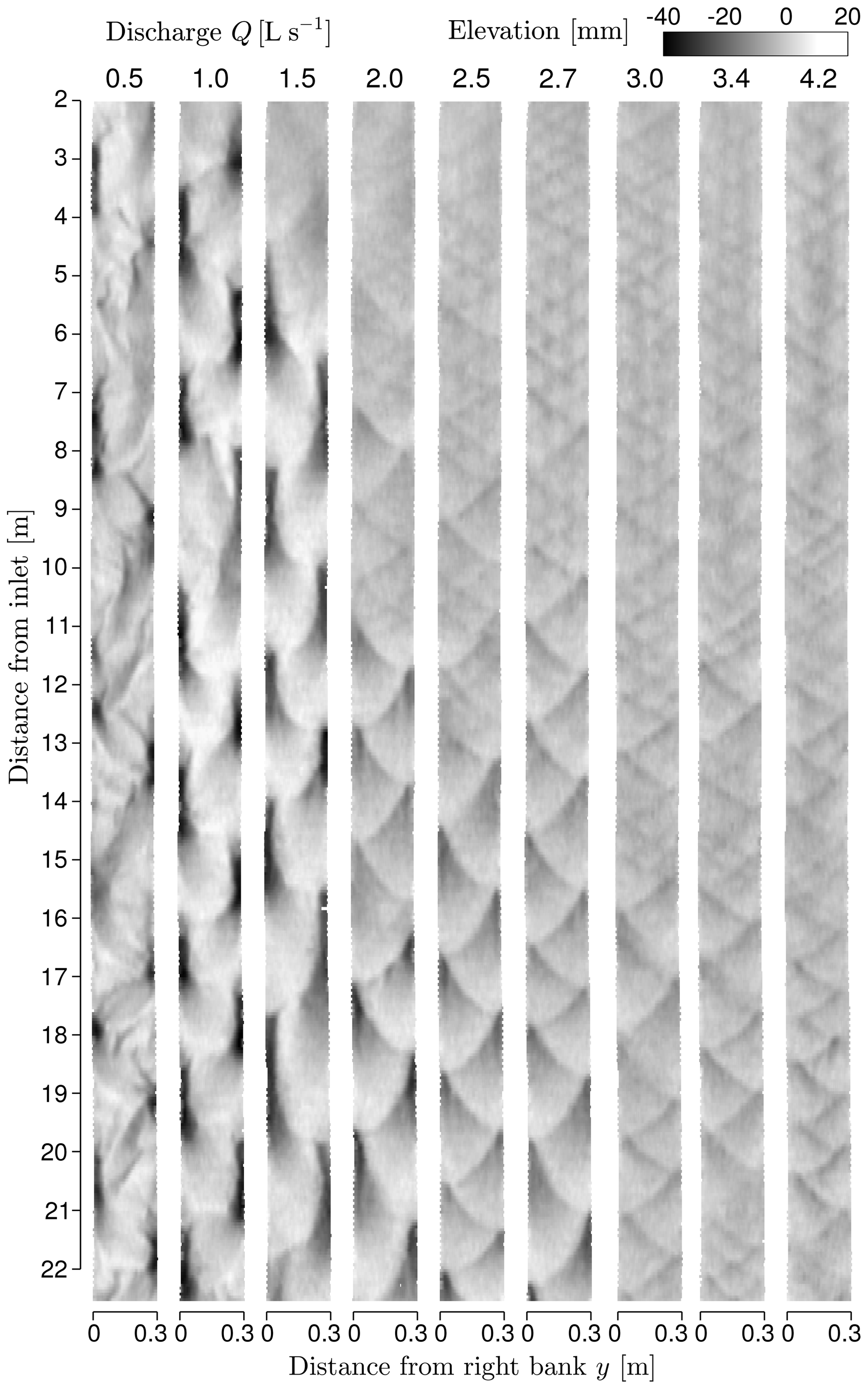
Figure 2 Maps of detrended bed elevation, showing the equilibrium bed morphology for increasing values of discharge. Flow is from top to bottom. The longitudinal scale is compressed for clarity.

3.1 Bar height and bed relief

A comparison of metrics for bar height and bed relief is presented in Fig. 3a and b. The bar height H_BM is maximum (almost 40 mm) for the $Q=\mathrm{1.0}\mathrm{L}{\mathrm{s}}^{-\mathrm{1}}$ run, then it gradually decreases with discharge until it attains a relatively constant value of about 13 mm for $Q\ge \mathrm{3.0}\mathrm{L}{\mathrm{s}}^{-\mathrm{1}}$. At the lowest discharge (0.5 L s⁻¹), bar height is lower than the peak value, showing a value around 33 mm. As expected, H_B is smaller than H_BM for all runs, but the difference is minimal and does not show a clear trend with discharge. An analogous behavior is observed for the bed relief metrics SD and BRI (Fig. 3b). Specifically, BRI tends to be only slightly smaller than SD, and both metrics exhibit a variation with discharge that follows the same trend observed for the bar height metrics H_BM and H_B. However, the variation of SD and BRI with discharge is less gradual, with bars formed at Q=1.0 and 1.5 L s⁻¹ showing distinctively higher values (nearly +50 %) than the other cases. In general, values of SD and BRI are much lower than H_BM and H_B, as bed relief metrics cover a range of values that is about one-fifth the observed range of bar height.

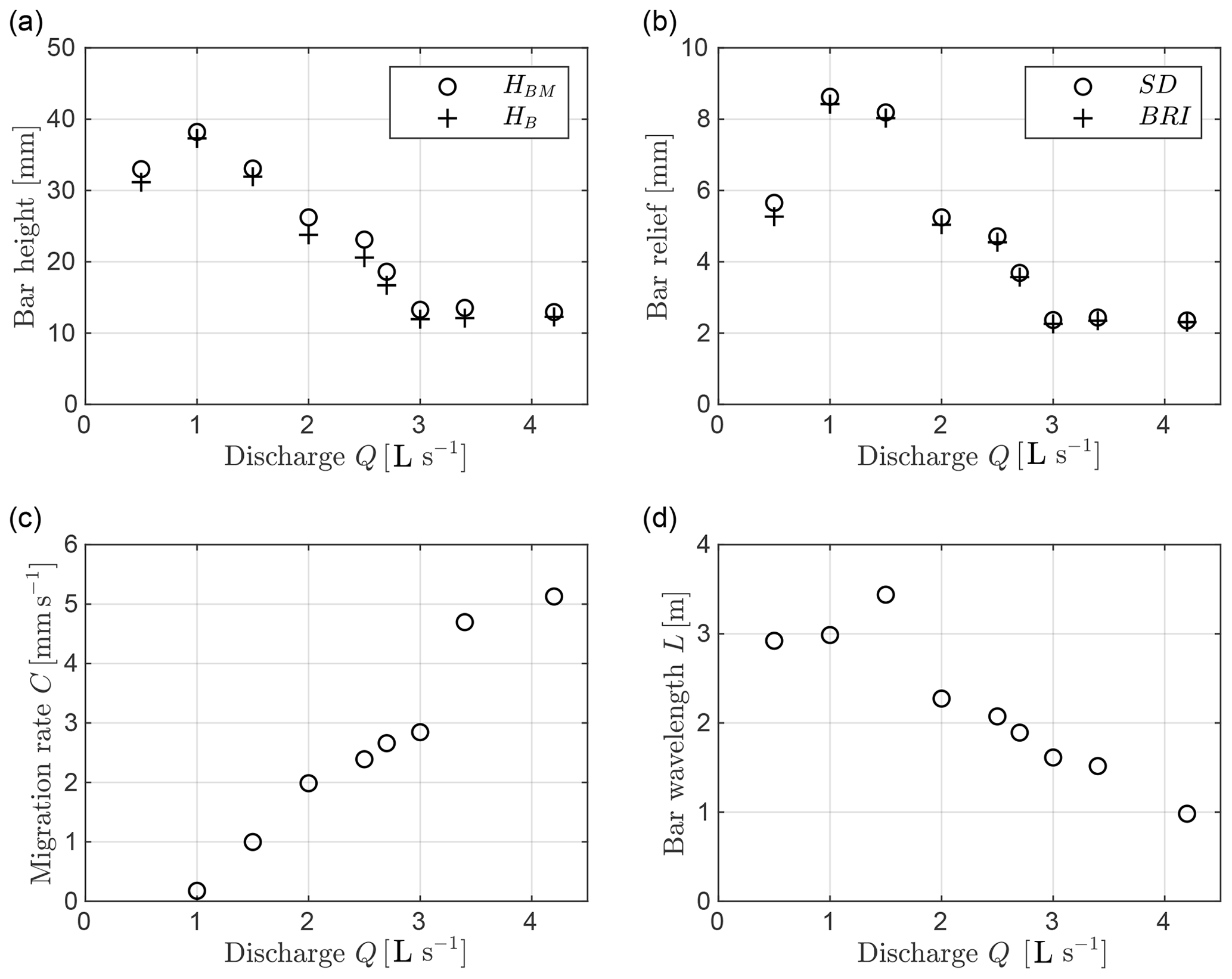
Figure 3 Mean properties of bars depending on discharge: (a) bar height H_BM and H_B; (b) bed relief, as measured by the standard deviation of the bed elevation distribution (SD) and the bed relief index (BRI); (c) bar migration rate C; (d) bar wavelength L.

Bars are downstream-migrating with a speed of the order of a few millimeters per second. At the lowest discharge, the migration rate was not measured because of the lack of easily recognizable fronts and the presence of complex patterns of erosion and deposition. For higher flows, the migration rate gradually increases from almost zero to 3 mm s⁻¹ for $Q=\mathrm{3.0}\mathrm{L}{\mathrm{s}}^{-\mathrm{1}}$ (see Fig. 3c), while between Q=3.0 and 3.4 L s⁻¹ it exhibits sudden growth to values around 5 mm s⁻¹. Mean bar wavelength (see Fig. 3d) is higher at low flows (∼3 to 3.5 m, corresponding to 10 to 12 channel widths) and decreases at higher discharges to approximately 1 m (about three channel widths). Specifically, the bar wavelength shows a rapid drop between Q=1.5 and 2.0 L s⁻¹, followed by a gradual decrease.

3.2 Predictions by the weakly nonlinear theory

The values of the equilibrium bar height predicted by the weakly nonlinear theory are reported in Fig. 4, which shows a decreasing trend of H_BM with the water discharge until it vanishes when the channel aspect ratio, β, matches its threshold value β_cr (no bars). Therefore, it is possible to define a corresponding threshold value of the flow discharge (a “critical discharge”, $Q_{\mathrm{cr}}=\mathrm{3.17}\mathrm{L}{\mathrm{s}}^{-\mathrm{1}}$), which separates the formative conditions for alternate bars (Q<Q_cr) from the region where bars do not develop (Q>Q_cr).

Figure 4 Bar height as a function of discharge according to the weakly nonlinear theory of Colombini et al. (1987). The solid line represents the equilibrium solution, while the dash–dot line indicates the bar height we obtained by limiting the bar growth to the fully wet condition. The development of alternate bars highly depends on discharge state with respect to the three key thresholds (vertical dashed lines), which represent (i) the critical condition of incipient sediment motion, $Q_{\mathrm{i}}=\mathrm{0.26}\mathrm{L}{\mathrm{s}}^{-\mathrm{1}}$, (ii) the condition for which bars at equilibrium are fully wet, $Q_{\mathrm{fw}}=\mathrm{1.26}\mathrm{L}{\mathrm{s}}^{-\mathrm{1}}$, and (iii) the critical condition for bar formation, $Q_{\mathrm{cr}}=\mathrm{3.17}\mathrm{L}{\mathrm{s}}^{-\mathrm{1}}$.

We note that the weakly nonlinear theory is formally valid near the critical conditions, although the comparison with experimental data suggests its applicability within a wider range of conditions (Colombini et al., 1987; Lanzoni, 2000b). However, at relatively low values of discharge, the predicted equilibrium elevation of the top of the bars would exceed the water surface elevation, which makes the equilibrium value of H_BM no longer meaningful. Therefore, when the discharge is smaller than the so-called fully wet threshold, Q_fw (see Adami et al., 2016), the system cannot reach equilibrium bar height. Under these conditions it is then reasonable to assume that bar growth stops as bar tops start to emerge, which means the maximum bar elevation must be set equal to the water surface elevation. This concept of emersion-limited bar height is represented by the dash–dot line in Fig. 4, which shows an opposite (i.e., increasing with the discharge) trend with respect to the theoretical equilibrium height. Ultimately, a lower limit of the region of possible bar formation is set by the flow discharge corresponding to incipient sediment motion, $Q_{\mathrm{i}}=\mathrm{0.26}\mathrm{L}{\mathrm{s}}^{-\mathrm{1}}$, which defines the third relevant threshold illustrated in Fig. 4.

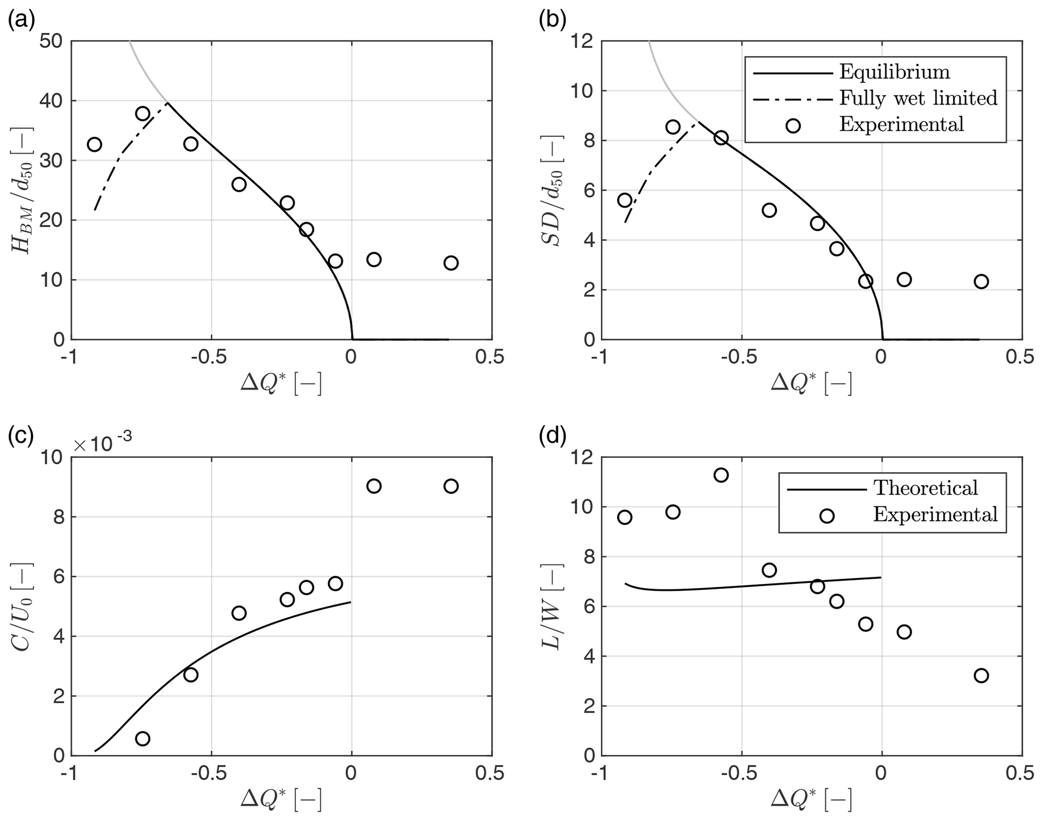
Figure 5 Dimensionless bar parameters as a function of the scaled discharge from theory (lines) and experiments (markers). (a, b) Height and standard deviation of bed elevation distribution (scaled with the median grain size d₅₀), with the solid line indicating equilibrium conditions and the dash–dot line representing the bar height limited by the fully wet condition. (c, d) Bar migration rate and wavelength (scaled with the flow velocity U₀ and the channel width W, respectively).

The theoretical response of bar height to varying flow conditions is then compared with the laboratory data, which gives the results illustrated in Fig. 5. Consistently with the theoretical analysis, all the metrics are represented in dimensionless form by scaling bar height and relief with the median grain size d₅₀, the bar wavelength by the channel width W, and the migration rate by the flow velocity U₀. Moreover, we define a dimensionless discharge as

$$\begin{array}{}\text{(10)}& \mathrm{\Delta }{Q}^{\ast }={\displaystyle \frac{Q-Q_{\mathrm{cr}}}{Q_{\mathrm{cr}}-Q_{\mathrm{i}}}},\end{array}$$

so that values from −1 to 0 cover the entire range of bar formation from the threshold of incipient sediment transport Q_i to the critical threshold Q_cr.

From this comparison it is apparent that bars observed at 3.4 and 4.2 L s⁻¹ are anomalous for a number of reasons: (i) they occur outside the region of bar formation (i.e., at Q>Q_cr), (ii) they exhibit a much faster migration rate, and (iii) their wavelength is much shorter with respect to the typically observed values (L=5–12 W; see Tubino et al., 1999). This type of bedform closely resembles the diagonal bars described by Jaeggi (1984) as three-dimensional mesoforms characterized by a wavelength of around 3 times the channel width, limited relief, symmetrical elevation distribution, and the presence of shallow pools. These bedforms were observed at Froude numbers close to 1 and did not match the region for alternate bar formation. Experimental observations by Jaeggi (1984) suggested that diagonal bars can be considered intermediate bedforms associated with the transition of dunes from two- to three-dimensional configurations. This idea was confirmed by the theoretical work of Colombini and Stocchino (2012), which provided an interpretation of diagonal bars as three-dimensional oblique dunes, distinct from alternate bars. Herein, we will therefore refer to bars observed at $\mathrm{\Delta }{Q}^{\ast }>\mathrm{0}$ as diagonal bars, reserving the term “alternate bars” for the remaining cases.

The analytical model reproduces both the bar height and the bed relief of alternate bars remarkably well (Fig. 5a and b). However, when the discharge approaches the critical threshold Q_i the weakly nonlinear model is no longer valid and the solution for the equilibrium amplitude diverges. As previously discussed, when discharge is lower than the fully wet threshold Q_fw the singularity of the analytical solution can be mitigated by considering the fully wet limited bar height, which provides a reasonable estimate of H_BM and SD. Similarly, the bar migration rate (Fig. 5c) is well-reproduced by the analytical model for both the overall trend and the absolute values, although the theory significantly overestimates the observed value at $Q=\mathrm{1.0}\mathrm{L}{\mathrm{s}}^{-\mathrm{1}}$. Furthermore, the theory properly predicts the wavelength of bars only for intermediate values of discharge (see Fig. 5d), while it does not capture the overall decreasing trend and therefore sharply underestimates the length of bars observed in the three runs with $Q\le \mathrm{1.5}\mathrm{L}{\mathrm{s}}^{-\mathrm{1}}$.

3.3 Quantitative analysis of the bar shape

In order to filter out the relatively small differences of single bar units, we computed for each discharge value an ensemble bar shape, defined as the average topography of all the bars formed under the same flow conditions. The resulting ensemble topographies represented in Fig. 6 show a rather regular pattern. We then analyzed the response of the bar shape to changing discharge by computing the skewness and the Fourier components of the ensemble bars for each discharge value.

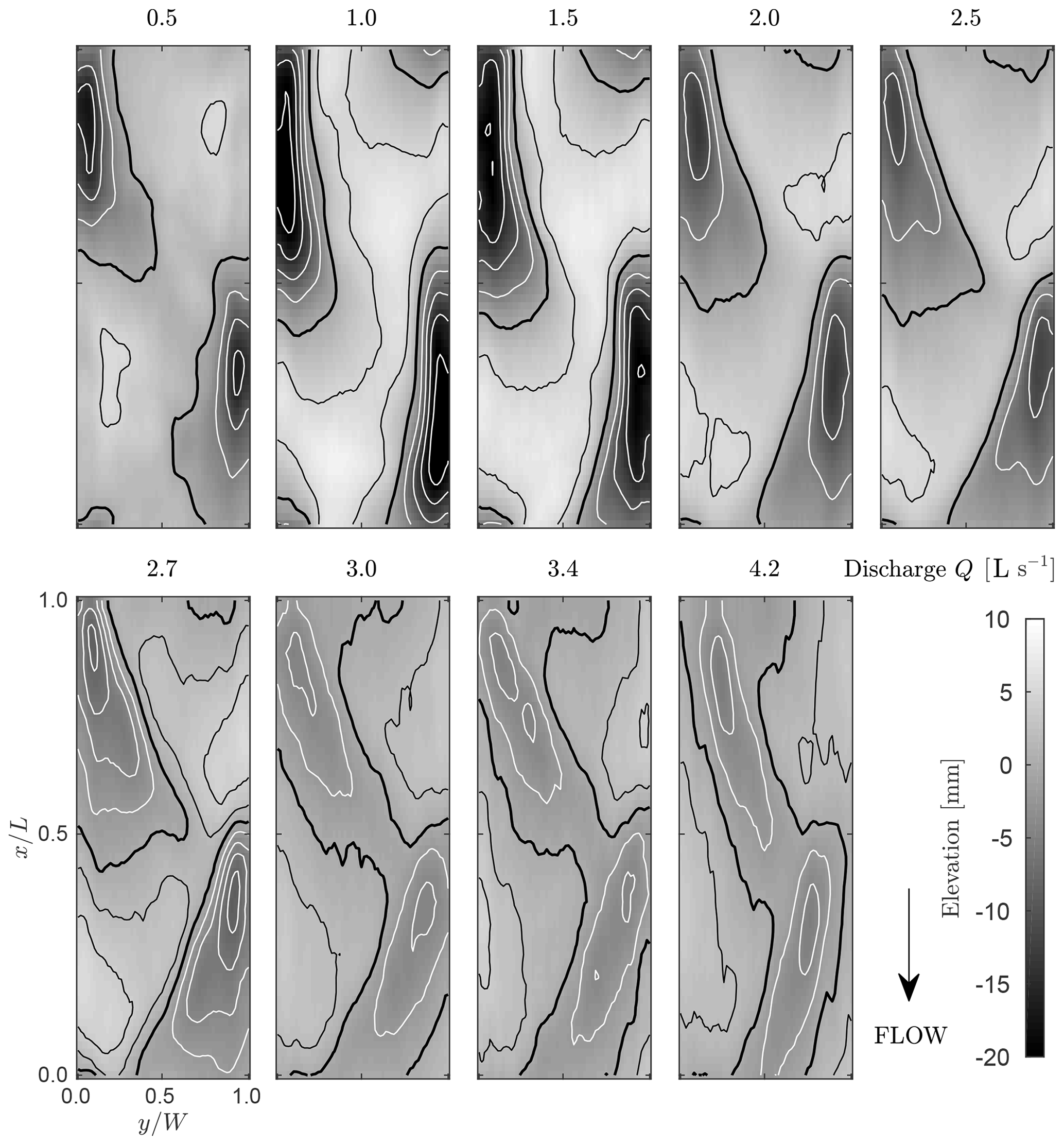
Figure 6 Maps of ensemble bars representing the variation of the average bar topography for increasing values of discharge. Spatial coordinates (x,y) are normalized with respect to the bar wavelength (L) and the channel width (W). Contour spacing is 5 mm (upper panels) and 2 mm (lower panels), with the thicker contour indicating the mean (i.e., zero) elevation and white contours representing negative elevation values. Flow is from top to bottom.

Figure 7 shows that the skewness is always negative, which indicates a left-tailed bed elevation distribution. For the lowest discharge the skewness is around −1.5, which matches typical values observed for wandering and braided channels (see Garcia Lugo et al., 2015). Highly negative values of the skewness are associated with the presence of narrow, deep troughs and wide, relatively flat bar crests that are clearly detectable in Fig. 6 for the ensemble bars at $Q\le \mathrm{1.5}\mathrm{L}{\mathrm{s}}^{-\mathrm{1}}$. This morphological characteristic becomes progressively less pronounced, as the ensemble bars corresponding to the range Q=2.5–3.0 L s⁻¹ show a comparable extension of regions of scour and deposition, as well as the presence of distinct diagonal fronts. The observed trend of the skewness parameter is in qualitative agreement with the theory, which predicts an increase from negative values at low flow to vanishing values (i.e., nearly symmetrical bed elevation distribution) when approaching the critical condition for bar formation (i.e., $\mathrm{\Delta }{Q}^{\ast }\simeq \mathrm{0}$). However, the magnitude of the observed skewness is much larger than the theoretical estimate due to the limited capability of the theoretical model to fully represent the complex, highly nonlinear morphodynamic processes (see Colombini et al., 1987).

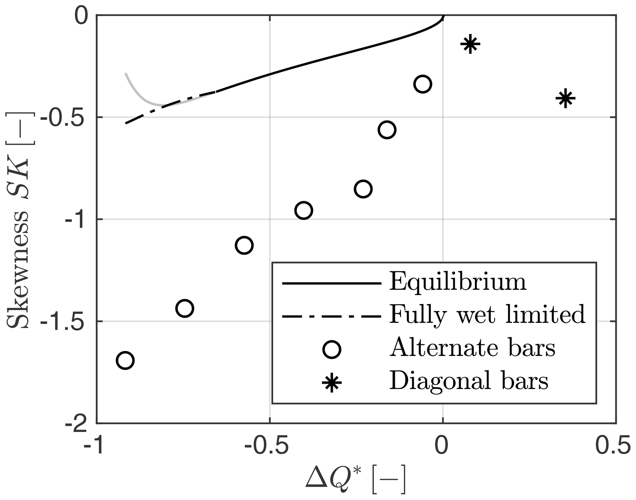
Figure 7 Skewness of the bed elevation distribution as a function of the scaled discharge. Markers indicate the skewness of the experimental ensemble bars; lines illustrate results from the weakly nonlinear theory, with the dash–dot line referring to the solution obtained by limiting the bar growth to the fully wet condition.

The analysis of the Fourier spectral composition of bed topography provides the amplitude of each component along the transverse and longitudinal direction. An example is shown in Fig. 8 for the ensemble bar of the $Q=\mathrm{2.5}\mathrm{L}{\mathrm{s}}^{-\mathrm{1}}$ run. The plot illustrates the amplitude of the first 36 (6×6) harmonic components, identified by their longitudinal (n) and transverse (m) mode. In this representation, n=1 indicates a complete sinusoidal period in one bar wavelength, while m=1 indicates half a wave period in one channel width. Harmonic components with n=0 and m=0 are constant along the x and y axis, respectively. The component A₀₀, which represents a horizontal plane, has an amplitude equal to zero because the original DEM was normalized by removing the mean. As revealed by their total energy content, E_n, the most important components of the spectrum are those with longitudinal mode n=1. Specifically, alternate bars are dominated by the component A₁₁, which represents a double sinusoidal bed deformation. Components with n=1 and higher, odd transverse mode m, such as the A₁₃ and the A₁₅, also appear in the spectrum, contributing to the deviation of the cross section from a purely sinusoidal variation to a more complex (but still antisymmetric) shape. However, components with longitudinal modes n=0 and n=2 are also relevant. The longitudinal mode n=0 is dominated by the component A₀₂, which represents a sinusoidal symmetric bed deformation that is constant in x, while the components with longitudinal mode n=2 include a number of (even) transverse modes (i.e., A₂₂, A₂₄), which represent a symmetric bed deformation that completes two periods in one bar wavelength (see Fig. 9 for a schematic representation). All m=0 harmonics, which represent a purely longitudinal bed deformation, turn out to be negligible, showing that the transversally averaged bed elevation is nearly zero for all the cross sections. Analogously, components with n=0 and odd transverse mode m are also vanishingly small, which implies that on average the bed structure does not exhibit any asymmetry with respect to the channel axis. For all tested conditions, the Fourier spectrum exhibits a clear checkerboard pattern within which at least 98 % of the energy is contained in even–even and odd–odd modes, while other harmonics have negligible power (on average 0.7 %). This distinctive pattern indicates that despite their morphological complexity, both alternate and diagonal bars are “purely alternate” in the sense that the second half of the bar is nearly identical to the first half but mirrored across the channel axis.

Figure 8 Amplitude of the first 6×6 longitudinal and transverse modes for the ensemble bar at $Q=\mathrm{2.5}\mathrm{L}{\mathrm{s}}^{-\mathrm{1}}$. Histograms on the bottom and on the right report the total energy E_n and E_m, representing the variance of the bed elevation associated with all the components having longitudinal mode n and transverse mode m, respectively.

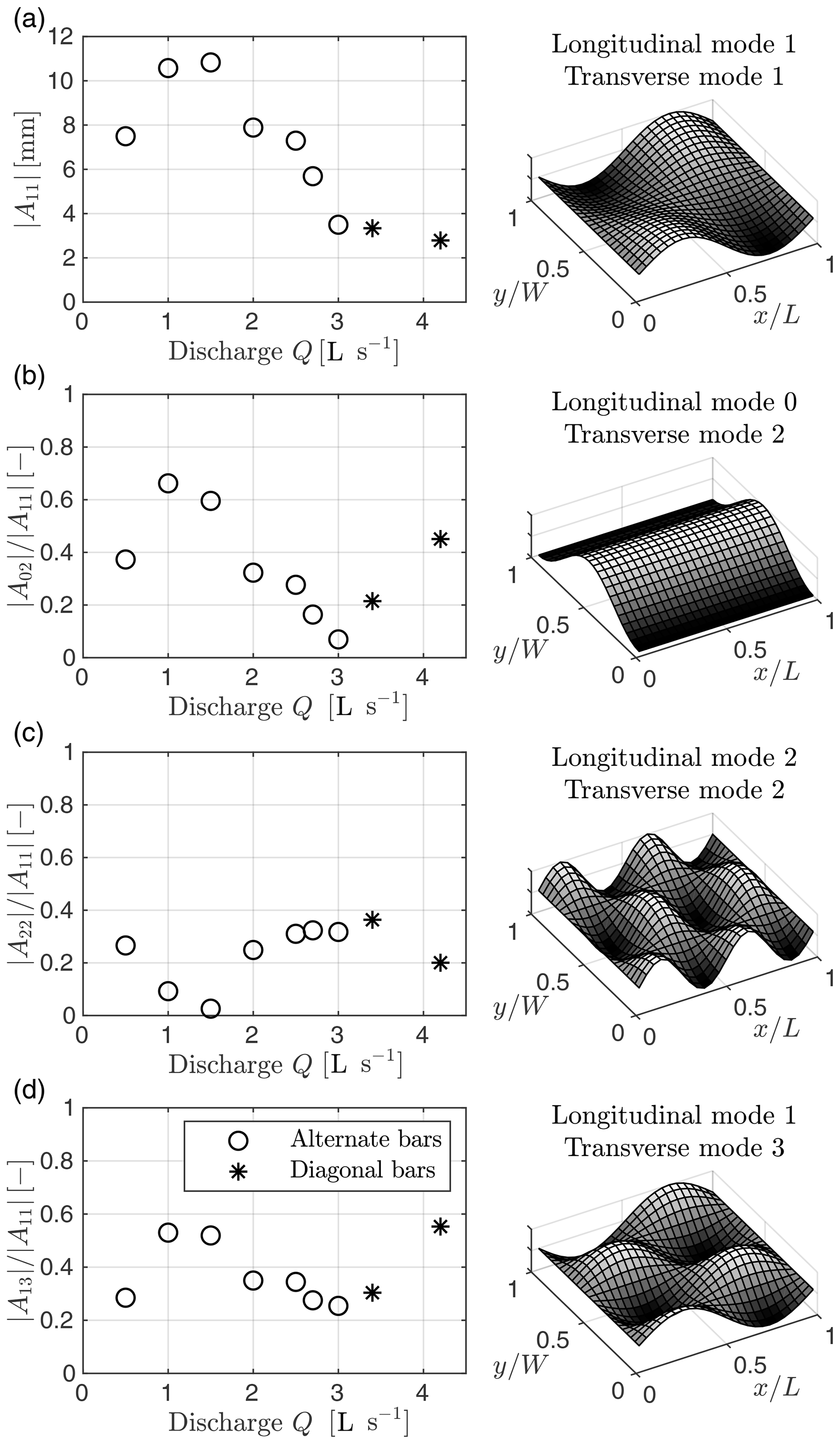
Figure 9 Amplitude of the main Fourier components depending on discharge. (a) Amplitude of the fundamental harmonic A₁₁. (b, c, d) Amplitude of the components A₀₂, A₂₂, and A₁₃ scaled with the amplitude of the fundamental. The 3-D plots on the right illustrate the bed deformation associated with each Fourier component.

We note that the above results are valid in general, regardless of the value of flow discharge. However, relevant variations of the Fourier spectrum composition occur when changing Q. The amplitude of the four dominant components A₁₁, A₀₂, A₂₂, and A₂₂ is illustrated in Fig. 9 as a function of the dimensionless discharge previously defined in Eq. (10). The amplitude of the fundamental harmonic, A₁₁, which is illustrated in Fig. 9a, closely follows the trend observed for bar height parameters (see Fig. 3a and b), with maximum values for Q=1.0 and 1.5 L s⁻¹, a steady decrease up to $Q=\mathrm{3.0}\mathrm{L}{\mathrm{s}}^{-\mathrm{1}}$, and lower, almost constant values afterwards. This is not surprising, as A₁₁ is the dominant component of the bed topography, which therefore mostly determines the bar height.

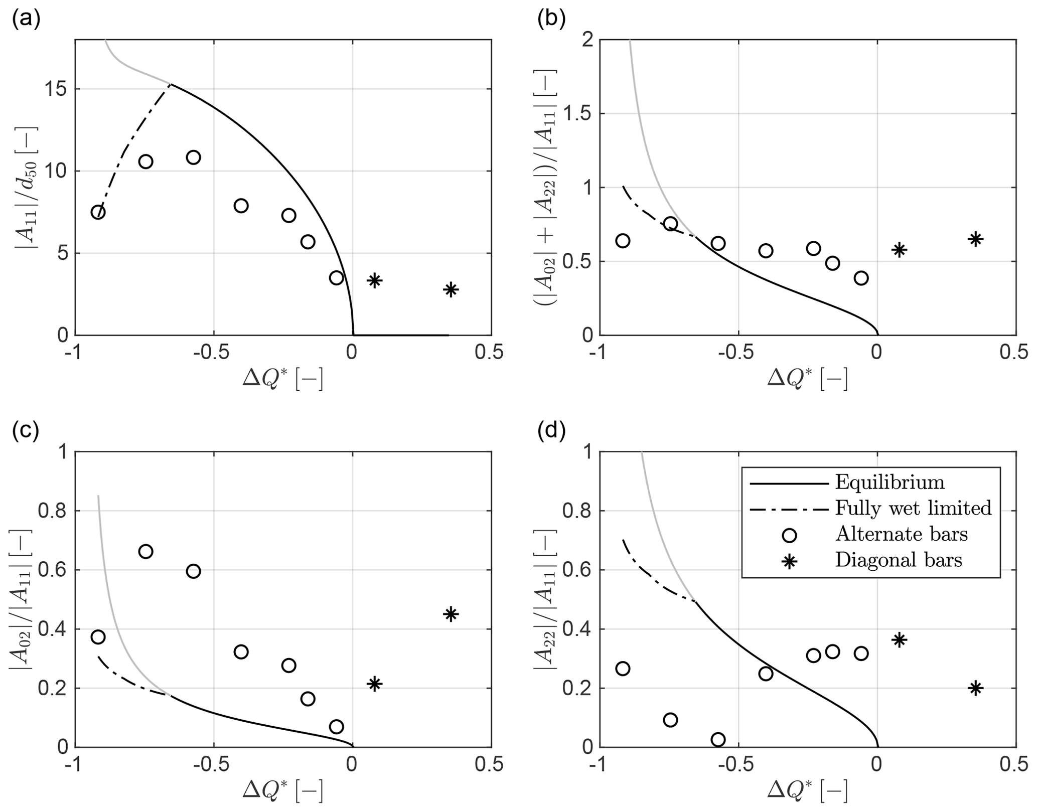
Figure 10 Amplitude of the main Fourier components depending on the scaled discharge from theory (lines) and experiments (markers). (a) Amplitude of the fundamental component A₁₁ scaled with the grain size d₅₀. (b, c, d) Amplitude of the m=2 components scaled with $\left|A_{\mathrm{11}}\right|$, with panel (b) reporting the sum of the absolute values of the coefficients A₀₂ and A₂₂ and panels (c, d) referring to the individual components A₀₂ and A₂₂. The solid line indicates theoretical results at equilibrium, while the dash–dot line indicates theoretical results obtained by limiting the bar growth to the fully wet condition.

To quantify the shape of the bars regardless of their absolute height, we then refer to the relative amplitude of the Fourier modes given as a proportion of the amplitude $\left|A_{\mathrm{11}}\right|$, as illustrated in Fig. 9b, c, and d. Excluding the first case ($Q=\mathrm{0.5}\mathrm{L}{\mathrm{s}}^{-\mathrm{1}}$), the trend observed for alternate bars is rather clear, with decreasing importance of both the symmetric component A₀₂ and the asymmetric component A₁₃ from amplitudes of about 60 %–70 % of $\left|A_{\mathrm{11}}\right|$ to significantly smaller values when approaching the critical threshold Q_cr. Specifically, the amplitude of the component A₀₂ decreases by about an order of magnitude. However, the component A₂₂ shows an inverse (i.e., increasing) trend from the nearly vanishing amplitude observed at Q=1.0 and 1.5 L s⁻¹ to values of about 1∕3 of $\left|A_{\mathrm{11}}\right|$ when approaching Q_cr. The weakly nonlinear theory of Colombini et al. (1987) resolves the first 2×2 modes of the Fourier spectrum, thus allowing for calculation of the expected variation of the main components illustrated in Fig. 9, except for A₁₃. The amplitude of the fundamental harmonic A₁₁ (Fig. 10b) is fairly well-reproduced, at least for values of the flow discharge that do not differ much from the critical threshold Q_cr, at which the theory is expected to work best. However, for lower discharge values the theoretical curve clearly overestimates the measured data, and the predicted equilibrium amplitude diverges as discharge approaches the threshold value Q_i. In this case, as also noticed earlier, an approximate solution can be derived by assuming that the bar growth is limited by the fully wet condition.

To investigate the overall importance of the m=2 components with respect to the fundamental, we first analyze the sum of the absolute values of the coefficients A₀₂ and A₂₂ scaled with the amplitude of the fundamental harmonic A₁₁. As illustrated in Fig. 10b, this metric tends to decrease with discharge, theoretically approaching zero near critical conditions (i.e., at $\mathrm{\Delta }{Q}^{\ast }\simeq \mathrm{0}$). Despite its limited capability to quantify fully nonlinear interactions, the theory allows for a proper estimation of the observed values. However, the main difference between theory and experimental data lies in the relative amplitude of the individual m=2 components, A₀₂ and A₂₂. As illustrated in Fig. 10c, the values of the ratio $\left|A_{\mathrm{02}}\right|/\left|A_{\mathrm{11}}\right|$ are strongly underestimated by the theory, with experimental values being roughly 4 times their theoretical counterparts. Conversely, values of the ratio $\left|A_{\mathrm{22}}\right|/\left|A_{\mathrm{11}}\right|$ reported in Fig. 10d are significantly overestimated. This indicates that the mode-2 component is not dominated by the presence of regular, periodic central bars (see map in Fig. 9c), as suggested by the theory, but it is mainly associated with a bell-shaped distortion of the average cross section (Fujita and Muramoto, 1985), as represented in Fig. 9b. Finally, the ratio $\left|A_{\mathrm{22}}\right|/\left|A_{\mathrm{11}}\right|$, illustrated in Fig. 10d, does not tend to zero as predicted by the theory. From a morphological point of view this implies that for Q→Q_cr, while “theoretical” bars tend to become purely sinusoidal (A₁₁ component only) as the solution approaches its linear limit, observed bars retain a certain degree of nonlinearity, showing a m=2 component that derives from the presence of clear diagonal fronts (see Fig. 6).

4 Discussion

4.1 Discharge and bar height

Experimental data reveal that bar height and relief generally decrease with increasing discharge and are therefore inversely correlated with the sediment transport rate. This finding, which at a first sight may appear counterintuitive, is a direct consequence of the decrease in channel aspect ratio for progressively higher flows that are typical of single-thread rivers. This implies that the largest bars tend to develop under moderate flow conditions in which discharge is high enough to mobilize the bed material and at the same time is sufficiently low with respect to the critical discharge for bar formation, Q_cr. The decreasing bed relief with discharge is expected to have a direct impact on the sediment transport rate. Specifically, for relatively low values of discharge the presence of bars can promote a transverse variability of the Shields number, which leads to a net increase in the sediment transport rate with respect to equivalent, flat bed conditions (e.g., Paola, 1996; Francalanci et al., 2012). This effect can mitigate the reduction of the average transport rate with decreasing discharge, thus making the sediment rating curve more linear (Ferguson, 2003; Redolfi et al., 2016).

Our results reveal that the weakly nonlinear model allows for reproducing the observed bar height both qualitatively and quantitatively. Despite the calibration of the parameter r, this is a significant result, as it highlights the capacity of the theoretical model to accurately capture the sharp decreasing trend of bar height from intermediate values of discharge to the critical threshold. However, the variation of the bar height with discharge is not monotone everywhere, as when discharge becomes relatively low, bars tend to emerge, and their relief tends to be reduced. In these conditions the equilibrium amplitude predicted by the Colombini et al. (1987) model is clearly unphysical. This is not surprising, as the theory assumes a simply connected domain, wherein the bed is fully submerged. To mitigate this issue, we propose a modified curve for the bar height obtained by limiting the growth of the bars by the fully wet condition. Situations in which bars emerge are expected to be more important for wider channels due to the larger range of discharge states between the threshold of incipient sediment transport and the fully wet threshold. Specifically, as the channel width-to-depth ratio grows, the equilibrium becomes increasingly complex, ultimately leading to wandering and braiding channels (see Ashmore, 2013; Garcia Lugo et al., 2015; Redolfi et al., 2016).

4.2 Discharge and bar shape

The definition of suitable metrics for quantifying variations of the bar shape allows us to highlight how the shape of alternate bars at equilibrium changes with discharge. The weakly nonlinear theory of Colombini et al. (1987), as well as the bar predictor of Crosato and Mosselman (2009), suggests that when discharge is relatively small (i.e., high width-to-depth ratio) the channel tends to form regular, periodic central bars (also called double-row bars; see Ikeda, 1984; Crosato and Mosselman, 2020) with scour and deposition equally distributed between the center of the channel and the area near the banks. However, as also evident from existing laboratory and numerical data (e.g., Fujita and Muramoto, 1985; Garcia Lugo et al., 2015; Qian et al., 2017; Cordier et al., 2019), it is clear that deposition preferentially occurs near the center of the channel (mid-channel bars), while deep pools are mostly concentrated near the banks. This produces a bell-shaped distortion of the average cross section, which gives a Fourier component A₀₂ that at low flows is far more important than the A₂₂ component. As highlighted by Colombini and Tubino (1991) this behavior can be explained by fully taking into account the nonlinear effects, which tend to be progressively more important when the channel aspect ratio increases. Moreover, mid-channel bars are typically not symmetric with respect to the channel centerline, but they often appear as compound bars, with the water flow mainly concentrating near the banks and sometimes cutting the entire channel width through the formation of channel bifurcations (e.g., Schuurman and Kleinhans, 2015; Duró et al., 2016). In experimental modeling of wandering and braided rivers (e.g., Ashmore, 1982; Garcia Lugo et al., 2015) the tendency of the channels to “stick to the banks” is often considered to be a side effect of the physical model. However, this may not necessarily be the result of a scaling issue, nor a consequence of the low roughness of the banks, but it could be associated with a natural tendency of the flow to follow the banks when they are sufficiently straight, with the bars mainly occupying the mid-part of the channel. The Fourier analysis also reveals that the component A₂₂ (as well as the A₁₃) does not vanish when approaching critical conditions, as the theory predicts. Considering that near Q_cr the weakly nonlinear analysis should provide an accurate solution of the shallow-water and Exner equations, this mismatch is likely to originate from the model equations themselves. Specifically, this may be related to three-dimensional effects, which could be locally important in determining the formation of relatively steep bar fronts that mark a significant difference with respect to the theoretical sinusoidal bed structure.

4.3 The observed transition between different types of bars

Experimental observations presented in this study provide detailed information on the relationship between bar characteristics and discharge, while other relevant channel properties, such as grain size and slope, are kept constant. Within the tested flow range, bars exhibit a variety of sizes and shapes and pass smoothly from one shape to the other as discharge increases. On the basis of their geometrical properties and migration rate it is possible to identify four main types of bars.

1. At low flows, when the channel aspect ratio is high, alternate bars are very irregular, and the channel tends to switch to a more complex, wandering morphology. Sediment transport occurs on a limited portion of the bed, and the bed evolution is not dominated by the downstream migration of bar fronts but rather by lateral erosion and cutoffs. This kind of bar is associated with conditions in which the top of the bars emerges so that the bed is not fully wet (W_w<W; see Table 1). The emersion limits the growth of the bar height and consequently restricts bed relief.

2. At low to intermediate flows, bars are clearly delineated and relief is high. Their transverse shape is highly asymmetric, with narrow, deep, elongated pools and high, flat bar tops occupying a large proportion of the cross section so that the elevation along the centerline of the channel is always above the median detrended elevation. The distribution of elevation is strongly negatively skewed, and the Fourier components A₀₂ (symmetrical deformation) and A₁₃ (asymmetrical deformation) are relatively strong. Bar fronts are clearly delineated, steep, and almost orthogonal to channel banks. Immediately downstream of fronts, where the deepest pools are located, there is no sediment in motion. Moreover, bar migration is slow and the wavelength is significantly higher than theoretically predicted values.

3. At intermediate to high flows, relief and bar wavelength decrease with increasing discharge, and bar fronts become curved and oblique. The bed elevation distribution is less skewed, and higher-order components of the Fourier spectrum become less relevant with respect to the fundamental harmonic A₁₁. As deep pools tend to disappear, sediment motion occurs on the entire channel surface. This kind of bed morphology represents the typical shape of alternate bars (i.e., that sketched in Fig. 1a) and shows a very close match with theoretical predictions in terms of height, wavelength, and migration rate.

4. Finally, at high flows diagonal bars form. Despite preserving an alternate shape, diagonal bars are rather different from alternate bars in terms of both geometrical properties and formation mechanism. The height of these bedforms is low and largely independent of discharge, and their elevation distribution is almost symmetrical. Diagonal bars are relatively short (less than five channel widths), with oblique, almost straight fronts that migrate downstream at high speed. They are observed outside the range of alternate bar formation (i.e., for Q>Q_cr) for discharge values that are also consistent with the empirical criterion proposed by Jaeggi (1984). According to Colombini and Stocchino (2012) diagonal bars are associated with the transition from two- to three-dimensional oblique dunes. This transition is expected when reducing the relative roughness d₅₀∕D, i.e., when approaching typical conditions of gravel bed rivers.

The three-dimensional character of the flow field is fundamental for explaining the morphology of diagonal bars. Specifically, when Q>Q_cr the two-dimensional, depth-averaged model of Colombini et al. (1987) would predict plane-bed conditions (no bars), while a three-dimensional, non-hydrostatic analysis is needed to reproduce the observed formation of diagonal bars (Colombini and Stocchino, 2012). For this reason, all depth-averaged numerical models for alternate bars (e.g., Crosato et al., 2011; Siviglia et al., 2013; Qian et al., 2017; Cordier et al., 2019) likely suffer from the same limitation. Since diagonal bars are of small amplitude, they are expected to have a limited effect on sediment transport and flow resistance. Moreover, they may easily disappear as a result of interaction with other more prominent bedforms (e.g., free alternate bars and forced bars) that are expected to form because of the natural variability of flow and channel geometry in rivers. Nevertheless, attention should be paid to the interpretation of numerical results and their comparison with field and laboratory observations.

From a visual inspection of the topographies illustrated in Fig. 2, it is evident that bars forming at $Q>\mathrm{2.0}\mathrm{L}{\mathrm{s}}^{-\mathrm{1}}$ are not spatially uniform, but they grow in the initial part of the channel before adapting to fully developed conditions. This behavior has been observed by laboratory and numerical experiments (Fujita and Muramoto, 1985; Defina, 2003; Nicholas, 2010; Qian et al., 2017) and has been associated with the fact that bar formation needs to be triggered by small perturbations, whose effect propagates downstream in the form of wave packages (i.e., trains of bars). Specifically, the spatial adaptation is probably a consequence of the convective (rather than absolute) nature of bar instability highlighted by Federici and Seminara (2003), which implies that the effect of local perturbations tends to be convected downstream rather than being spread throughout the whole domain.

On the basis of theoretical results, it is possible to define an additional threshold value of discharge corresponding to conditions in which the channel aspect ratio β equals the resonant value β_res, originally defined by Blondeaux and Seminara (1985) (see Table 1). We name this threshold value “resonant discharge” (Q_res), which turns out to equal 1.94 L s⁻¹. Although not directly affecting the theoretical solution for free migrating bars, the resonant threshold is fundamental for defining the propagation of morphological effects that can be generated by any flow disturbance (e.g., that associated with boundary conditions). Specifically, as first highlighted by Zolezzi and Seminara (2001), under sub-resonant conditions (i.e., Q>Q_res) morphological effects tend to manifest themselves downstream of the disturbance, while an upstream propagation is possible in the super-resonant regime (i.e., when Q<Q_res). The different behavior of bars observed at relatively low flows, which tend to be well-developed along the entire flume (see Fig. 2), may be associated with the super-resonant character of the experiments. In this case the possible upstream propagation of the morphological information may favor an upstream diffusion of the bed instability, which can therefore reach the initial part of the channel.

4.4 The alternate nature of both alternate bars and diagonal bars

The checkerboard pattern of the Fourier spectra indicates that both alternate and diagonal bars are purely alternate in the sense that the elevation map of the upstream half-wavelength is nearly identical to the downstream half but mirrored along the channel centerline. Note that this does not imply a point symmetry with respect to the center of the bar ($y=W/\mathrm{2}$ and $x=L/\mathrm{2}$) but rather a switching of the same erosion and deposition pattern between the two sides of the channel. Interestingly, this is valid even for the ensemble bars at the lowest discharge ($Q=\mathrm{0.5}\mathrm{L}{\mathrm{s}}^{-\mathrm{1}}$), despite the complexity of the bed topography displayed in Fig. 2.

This particular pattern is intrinsically linked to bar formation mechanisms. To some extent, both alternate and diagonal bars can be considered free bars in the sense that they both arise from an autogenic, three-dimensional instability of the erodible bed. This kind of instability does not break the overall symmetry of the problem; therefore, if a deposition patch tends to form near one bank, a similar feature should appear somewhere else but on the opposite side of the channel. This suggests that if periodic, three-dimensional bedforms develop, they should follow an alternate pattern, at least in an average statistical sense.

From a mathematical point of view, the checkerboard pattern can be explained by considering the fact that free bars tend to initially appear as a bed deformation having a double sinusoidal shape (A₁₁ component only), while as they grow, nonlinear interactions gives rise to the second-order A₀₀, A₀₂ A₂₀, and A₂₂ harmonics (see Colombini et al., 1987; Bertagni and Camporeale, 2018). Extending the analysis to a higher-order approximation would give other even–even and odd–odd modes but no mixed even–odd and odd–even components.

Finally, it is worth noting that the dominance of the even–even and odd–odd modes has an experimental significance, as it indicates that (i) there are no systematic trends associated with channel asymmetries (e.g., product of initial bed leveling), and (ii) random effects resulting from measurement errors, experimental imperfections, or the intrinsic stochasticity of sediment transport processes are not significantly affecting the shape of the ensemble bar.

4.5 Suitable metrics for quantifying bar height and relief

The laboratory dataset used for this work allowed for the comparison of a number of methods and metrics to characterize bar height and relief. Historically, interest in the quantification of bar height arose from the influence of bars on human activities and interaction with artificial structures (Jaeggi, 1984). Therefore, maximum scour and deposition were the most relevant parameters utilized to evaluate the risk of levee instability and levee overtopping, respectively. However, metrics of bar height based on maxima and minima (H_BM and H_B) are highly sensitive to measurement errors and uncertainties that derive from the presence of vegetation on the bar top and from the difficulty of measuring the bottom elevation in deep pools. Moreover, the estimation of both H_BM and H_B requires the identification of individual bar units, which introduces potential sources of uncertainties and limits its application to bed configurations in which a dominant longitudinal wavelength is clearly recognizable.

Comparatively, SD and BRI are robust indices that do not depend on extreme values of elevation but on the entire bed elevation distribution. Moreover, these bed relief metrics can be applied to a range of different morphologies, thus allowing for comparisons between bars and other bedforms. Since SD and BRI show the same trend observed for H_BM and H_B, the former can provide better data when the purpose is not to quantify the maximum scour and deposition but rather to measure morphological trajectories and to compare study cases with experimental and numerical simulations.

It is also important to note that metrics based on the comparison of elevation values at different longitudinal positions (i.e., H_BM and SD) require detrending the bed elevation by removing an average slope that is often not obvious to define. Our experiments show that results are very similar when instead considering the cross-section-based indices H_B and BRI, with the advantage that they are fully independent of how the average slope is detrended. This similarity is linked to the presence of deep, small pools and large, flat bar tops. Cross-sectional relief is more strongly influenced by the former, and the maximum elevation along the cross section where the lowest point is located is not very different from the highest point of the entire bar.

5 Conclusions

We explored how the equilibrium properties of free migrating alternate bars depend on water discharge through a series of laboratory experiments, wherein width, channel slope, and bed material were kept constant. A proper definition of the most suitable metrics, the analysis of the experimental results, and the comparison with existing theoretical models allow us to draw the following conclusions.

1. The equilibrium bar height generally decreases with increasing discharge. However, at low flows, when bars start emerging from the water surface, an opposite trend is observed, which implies that moderate flows are mainly responsible for the formation of large alternate bedforms.

2. The shape of alternate bars significantly changes with discharge; relatively low flow conditions are characterized by a high negative skewness of the bed elevation distribution and an important contribution of the higher-order Fourier modes with respect to the fundamental harmonic.

3. At low discharge, when the width-to-depth ratio is relatively high, the mode-2 Fourier components become increasingly important. However, the channel does not tend to develop regular central bars but rather a bell-shaped distortion of the average cross section, with deposition preferentially occurring near the center of the channel (mid-channel bars) and scour pools mainly located near the banks.

4. The significant variations of the bar morphology and the associated metrics allow for identifying four main types of bars, which are associated with different flow conditions with respect to the relevant morphodynamic thresholds.

5. The weakly nonlinear theory allows for a satisfactory prediction of bar height and migration speed, while its capability to reproduce the bar shape is limited to a qualitative analysis. Moreover, limiting the bar growth to the fully wet condition allows for correcting the theoretical predictions at low values of discharge, at which alternate bars tend to emerge from the water surface.

6. The transition from alternate bar morphology to a plane-bed configuration that is expected when discharge exceeds the critical threshold Q_cr is not sharp due to the formation of diagonal bars, which should be regarded as three-dimensional oblique dunes.

7. The definition of ensemble bars that represent the average bar topography clearly highlights the purely alternate character of both alternate bars and diagonal bars, which manifests itself as a checkerboard pattern of the Fourier spectrum. In general, our definition of ensemble topography can be used for analyzing any quasi-periodic morphological pattern, such as curvature-driven point bars forming in meandering rivers.

Appendix A: Calculation of Fourier coefficients

Here we detail the procedure needed to expand the signal in the form of Eq. (5) and to calculate the associated coefficients A_nm. We start by considering a generic real-valued, two-dimensional signal f_jk defined on a regular grid of J×K points, whose indexes j and k run from 0 to J−1 and from 0 to K−1, respectively. The two-dimensional, discrete Fourier transform allows for expressing the signal as follows:

$$\begin{array}{}\text{(A1)}& f_{jk}=\sum _{m=\mathrm{0}}^{J-\mathrm{1}}\sum _{n=\mathrm{0}}^{K-\mathrm{1}}{F}_{nm}\exp \left[\mathrm{2}\mathit{\pi }in{\displaystyle \frac{j}{J}}+\mathrm{2}\mathit{\pi }im{\displaystyle \frac{k}{K}}\right],\end{array}$$

where i is the imaginary unit, and the complex Fourier coefficients F_nm can be calculated through standard fast Fourier transform algorithms (e.g., the MATLAB FFT2 function).

Considering the L×W domain illustrated in Fig. A1, with the system of reference (x,y) originating at the lower left corner, the coordinates of the grid points can be determined as $x=(j+\mathrm{0.5})\mathrm{d}x$ and $y=(k+\mathrm{0.5})\mathrm{d}y$, where $\mathrm{d}x=L/J$ and $\mathrm{d}y=W/K$ are the grid spacing in the longitudinal and transverse directions, respectively. In this system of reference, the Fourier expansion of the signal can be expressed as

$$\begin{array}{}\text{(A2)}& f_{jk}=\sum _{m=\mathrm{0}}^{J-\mathrm{1}}\sum _{n=\mathrm{0}}^{K-\mathrm{1}}{F}_{nm}^{\ast }\exp \left[\mathrm{2}\mathit{\pi }in{\displaystyle \frac{x}{L}}+\mathrm{2}\mathit{\pi }im{\displaystyle \frac{y}{W}}\right],\end{array}$$

whose Fourier coefficients can be readily computed as

$$\begin{array}{}\text{(A3)}& F_{nm}^{\ast }=F_{nm}\exp \left[-\mathit{\pi }i\left({\displaystyle \frac{n}{J}}+{\displaystyle \frac{m}{K}}\right)\right].\end{array}$$

Figure A1 Illustration of the grid used to discretize a domain of size L×W, where W is the channel width. Grid points are identified by the indexes j and k (x and y direction, respectively) and are equally spaced at intervals dx and dy. The original grid contains J×K points (closed circles), while the extended grid, obtained by adding virtual external points (open circles), is formed by J×2K points that cover a total width 2W.

Equation (A2) contains both sines and cosines in both the x and y directions, as evident when expanding the complex exponential by means of the Euler's identity:

$$\begin{array}{}\text{(A4)}& \begin{array}{rl}{f}_{jk}& =\sum _{m=\mathrm{0}}^{J-\mathrm{1}}\sum _{n=\mathrm{0}}^{K-\mathrm{1}}{F}_{nm}^{\ast }[\cos \left(\mathrm{2}\mathit{\pi }n{\displaystyle \frac{x}{L}}\right)\cos \left(\mathrm{2}\mathit{\pi }m{\displaystyle \frac{y}{W}}\right)\\ & -\sin \left(\mathrm{2}\mathit{\pi }n{\displaystyle \frac{x}{L}}\right)\sin \left(\mathrm{2}\mathit{\pi }m{\displaystyle \frac{y}{W}}\right)\\ & +i\cos \left(\mathrm{2}\mathit{\pi }n{\displaystyle \frac{x}{L}}\right)\sin \left(\mathrm{2}\mathit{\pi }m{\displaystyle \frac{y}{W}}\right)\\ & +i\sin \left(\mathrm{2}\mathit{\pi }n{\displaystyle \frac{x}{L}}\right)\cos \left(\mathrm{2}\mathit{\pi }m{\displaystyle \frac{y}{W}}\right)].\end{array}\end{array}$$

Here we are interested in obtaining an expression in which, consistently with theoretical analyses (e.g., Colombini et al., 1987), only cosines appear in the transverse structure. To obtain such an expression, we start by considering the fact that the signal f_ij can be represented in a different way by adding virtual external points at which arbitrary values are assigned to the signal. This technique is rather common in signal analysis to obtain a different Fourier representation of the same signal: for example, a zero padding is often used to increase the wavelength of the fundamental harmonic. Specifically, if we extend the grid by adding K virtual points in the y direction as illustrated in Fig. A1 and we compute the Fourier transform as detailed above, we obtain the following expression:

$$\begin{array}{}\text{(A5)}& f_{jk}=\sum _{m=\mathrm{0}}^{J-\mathrm{1}}\sum _{n=\mathrm{0}}^{\mathrm{2}K-\mathrm{1}}{F}_{nm}^{\ast }\exp \left[\mathrm{2}\mathit{\pi }in{\displaystyle \frac{x}{L}}x+\mathrm{2}\mathit{\pi }im{\displaystyle \frac{y}{\mathrm{2}W}}\right],\end{array}$$

which is similar to Eq. (A2), except for the transverse wavelength of the fundamental harmonic being twice the channel width (2W). The key to eliminating the sine components along the y direction is to properly assign the values of f_ij at the virtual points. Specifically, if the signal is mirrored with respect to the y=W axis, the sum of all the terms containing sin (y) identically vanishes so that the Fourier expansion (A5) can be written as follows:

$$\begin{array}{}\text{(A6)}& \begin{array}{rl}{f}_{jk}& =\sum _{m=\mathrm{0}}^{J-\mathrm{1}}\sum _{n=\mathrm{0}}^{\mathrm{2}K-\mathrm{1}}{F}_{nm}^{\ast }\cos \left(\mathrm{2}\mathit{\pi }m{\displaystyle \frac{y}{W}}\right)[\cos \left(\mathrm{2}\mathit{\pi }n{\displaystyle \frac{x}{L}}\right)\\ & +i\sin \left(\mathrm{2}\mathit{\pi }n{\displaystyle \frac{x}{L}}\right)].\end{array}\end{array}$$

Equation (A6) contains redundant information, as components actually having an identical structure appear more than once in the sum. Specifically, it is possible to demonstrate that only M×N components are needed to exactly represent a real signal, where N=K and M equals $J/\mathrm{2}+\mathrm{1}$ or $(J+\mathrm{1})/\mathrm{2}$, depending on J being an even or an odd number, respectively. Therefore, a proper definition of the coefficients A_nm allows for expanding the signal f_ij in the following parsimonious way:

$$\begin{array}{}\text{(A7)}& \begin{array}{rl}{f}_{jk}& =\sum _{m=\mathrm{0}}^{M-\mathrm{1}}\sum _{n=\mathrm{0}}^{N-\mathrm{1}}\cos \left(\mathrm{2}\mathit{\pi }m{\displaystyle \frac{y}{\mathrm{2}W}}\right)\mathit{\text{Re}}\mathit{\left\{}{A}_{nm}\right[\cos \left(\mathrm{2}\mathit{\pi }n{\displaystyle \frac{x}{L}}\right)\\ & +i\sin \left(\mathrm{2}\mathit{\pi }n{\displaystyle \frac{x}{L}}\right)\left]\mathit{\right\}},\end{array}\end{array}$$

which can be equivalently written in the form of Eq. (5) after expressing the complex coefficients in terms on their amplitude and phase:

$$\begin{array}{}\text{(A8)}& A_{nm}=\left|A_{nm}\right|\exp \left(i{\mathit{\varphi }}_{nm}\right).\end{array}$$

The Fourier coefficients A_mn can be directly derived from the $F_{nm}^{\ast }$ coefficients and can be computed for a generic f_jk signal using the MATLAB code we made available at https://bitbucket.org/Marco_Redolfi/fourier_transform_bars (last access: 18 September 2020).