Complementing scale experiments of rivers and estuaries with numerically modelled hydrodynamics

Physical scale experiments enhance our understanding of fluvial, tidal and coastal processes. However, it has proven challenging to acquire accurate and continuous data on water depth and flow velocity due to limitations of the measuring equipment and necessary simplifications during post-processing. A novel means to augment measurements is to numerically model flow over the experimental digital elevation models. We investigated to what extent the numerical hydrodynamic model Nays2D can reproduce unsteady, nonuniform shallow flow in scale experiments and under which conditions a model is preferred to measurements. To this end, we tested Nays2D for one tidal and two fluvial scale experiments and extended Nays2D to allow for flume tilting, which is necessary to steer tidal flow. The modelled water depth and flow velocity closely resembled the measured data for locations where the quality of the measured data was most reliable, and model results may be improved by applying a spatially varying roughness. The implication of the experimental data–model integration is that conducting experiments requires fewer measurements and less post-processing in a simple, affordable and labour-inexpensive manner that results in continuous spatio-temporal data of better overall quality. Also, this integration will aid experimental design.

1 Introduction

Physical scale experiments greatly enhance our understanding of fluvial, estuarine and coastal processes and complement field observations and numerical models. The benefits of experiments that complement the other two means of research are twofold. Firstly, real material is used with its inherent laws and properties, as opposed to numerical models that require many parameters and approximations of laws for water flow, sediment transport (e.g. Meyer-Peter and Müller, 1948; Van Rijn, 2007; Baar et al., 2019) and life forms (e.g. Baptist et al., 2007; Van Oorschot et al., 2016). Secondly, experiments enable full control of the initial and boundary conditions and require little time to form entire systems, as opposed to the slow, ever-changing nature observed remotely or in the field.

The focus of this study is on landscape scale experiments that simulate morphodynamics with shallow water depths of maximally a few centimetres, i.e. in or just above the viscous sublayer. This kind of scale experiments differs from classical hydraulic flume studies (e.g. Struiksma et al., 1985; Neary et al., 1999) and larger-scale experiments (e.g. Zanichelli et al., 2004; Siviglia et al., 2013) with water depths >10 cm in which flow data can be more easily measured with lasers and submerged flow meters (e.g. ADCP). In contrast, data collection in landscape experiments is often difficult, infrequent and hindered by various problems (Fig. 1).

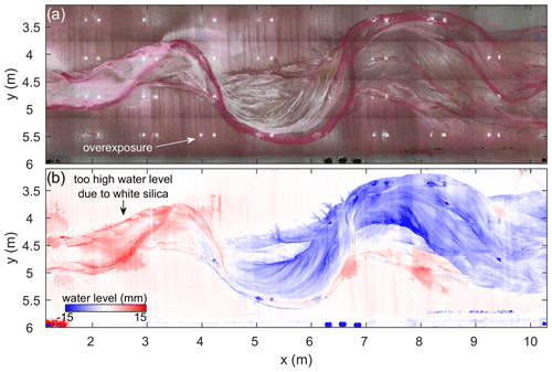
Figure 1 Exemplary data of a physical scale experiment of a meandering river by Van Dijk et al. (2013a) show how data extraction may be distorted. (a) Overhead imagery shows cases of light overexposure and the distribution of white silica flour. The water is dyed red where the water colour saturation is a measure of water depth. Flow is from left to right. (b) Water levels, based on measured bed elevations and water depths estimated from water colour saturation, are too high above the floodplain (z=0 mm) at locations of abundant silica flour and too low at locations of overexposure.

Typical data collection in such experiments targets the following three elements: (1) the morphological development from overhead imagery and digital elevation models (DEMs) from laser scanning or stereo photography on a dry bed (e.g. Ashworth et al., 2004; Hoyal and Sheets, 2009; Leduc et al., 2019); (2) water depth estimated from dye and light attenuation, possibly combined with absolute water level point measurements (e.g. Peakall et al., 2007; Tal and Paola, 2007, 2010); and (3) flow velocity from particle imaging velocimetry on the water surface from floating particles or dye injections (e.g. Tambroni et al., 2005; Braudrick et al., 2009). Due to the shallow water depths in landscape experiments, it is technically difficult to conduct flow measurements by submerged instruments without disturbance of the sediment transport and with the same spatial resolution as the bathymetry. To overcome the drawbacks of data collection and post-processing, so far only one research team (Tesser et al., 2007; Stefanon et al., 2010, 2012) has modelled water depth and flow velocity over DEMs of tidal basin scale experiments. However, the modelled data acquired by this novel method were not extensively validated against measured data, and the model only applied for uniform flow conditions (Marani et al., 2003).

Here we explore the possibility of extending the numerical flow model application by Tesser et al. (2007) and Stefanon et al. (2010, 2012) for unsteady, nonuniform flows in landscape scale experiments. We aim to complement the measured morphological data with continuous, spatio-temporally dense numerical data of water depth, flow velocity and bed shear stress. On the one hand, this is a similar practice to modelling flow over the measured morphology of real rivers and estuaries (e.g. Berends et al., 2019), whilst here the shallow-water equations need to be solved. On the other hand, this practice differs from remodelling the morphological development of a scale experiment (e.g. Struiksma et al., 1985), which are subject to all the combined errors of sediment transport predictors (Baar et al., 2019). The extended integration of experimental data and a numerical model would not only expand the possibilities for data analyses of a series of experiment bed scans but would also open up fast methods of testing alternative experimental settings for either an experimental or idealised morphology. This would save valuable time in the laboratory, especially for long-lasting experiments that include vegetation (e.g. Braudrick et al., 2009; Van Dijk et al., 2013b; Lokhorst et al., 2019).

Friedkin (1945)Schumm and Khan (1972)Schumm et al. (1987)Ashmore (1991a, b)Ashworth et al. (1994)Gran and Paola (2001)Ashworth et al. (2004)Peakall et al. (2007)Tal and Paola (2007, 2010)Hoyal and Sheets (2009)Van Dijk et al. (2009)Braudrick et al. (2009)Gardner and Ashmore (2011)Van Dijk et al. (2012, 2013a)Van Dijk et al. (2013b)Van de Lageweg et al. (2013, 2014)Leduc et al. (2019)Reynolds (1889, 1891)Mayor-Mora (1977)Tambroni et al. (2005)Tesser et al. (2007)Stefanon et al. (2010, 2012)Vlaswinkel and Cantelli (2011)Kleinhans et al. (2012, 2015)Iwasaki et al. (2013)Kleinhans et al. (2014)Braat et al. (2018)Leuven et al. (2018)Leuven and Kleinhans (2019)

Table 1 Data collection techniques in fluvial and tidal scale experiments with erodible boundaries and flows shallower than a few centimetres. “Overhead imagery” constitutes imagery or video from a camera at a fixed position that potentially allows for the classification of the experiment planform. Water depths “est. from physics” are determined for a few cross sections assuming uniform flow and a given discharge. “SfM” is structure-from-motion photogrammetry. The field “Remarks” contains additional sediments/vegetation on top of the main sediment that may interfere with overhead imagery analyses.

2 Review: experimental data collection and post-processing techniques

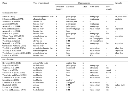
In order to quantify the hydro- and morphodynamics of a landscape scale experiment with shallow flow, the following three data types are commonly measured: dry bed elevation, water depth and flow velocity (Table 1). Below, the data collection and post-processing methods of these data are presented in conjunction with their drawbacks and achievable level of accuracy.

Firstly, bed elevation of experiments can be acquired through numerous techniques. These include a water level contour survey (Reynolds, 1889, 1891), a manual/digital point gauge survey (e.g. Friedkin, 1945; Peakall et al., 2007), 3D/laser and structured light (zSnapper^®) scanning (e.g. Gran and Paola, 2001; Tambroni et al., 2005; Van de Lageweg et al., 2014; Kleinhans et al., 2014; Marra et al., 2014), ultrasonic echo sounding (e.g. Best and Ashworth, 1994; Hoyal and Sheets, 2009; Stefanon et al., 2010, 2012), and structure-from-motion (SfM) photogrammetry through which photos are georeferenced to ground control points (Agisoft PhotoScan) (e.g. Westoby et al., 2012; Leduc et al., 2019). The most accurate technique is the point gauge survey (±0.1 mm) (Best and Ashworth, 1994), which does not require the flume to be drained. However, point gauging is terribly slow to get full coverage, as is the case for the water level contour survey, in which dry bed–water boundaries are registered for different water levels (Reynolds, 1889, 1891). In contrast, scanning, sounding and photogrammetry are much quicker and typically result in a vertical accuracy of ±0.5 to 1 mm (Peakall et al., 2007; Leduc et al., 2019). Yet, these three techniques require a dry bed, apart from a few kinds of laser scanners (Tesser et al., 2007; Stefanon et al., 2010, 2012). Consequently, the bed may be disrupted during the draining and refilling of the flume. Also, vegetation hampers their accurate reading of the bed elevation (e.g. Gran and Paola, 2001). In consequence of these drawbacks, the number of DEMs is usually limited.

Secondly, water depth maps are acquired while the experiment runs in either of two approaches: water depth is derived from the dyed water colour saturation or from measured water levels. As for the first approach on dye, the water colour saturation is an indicator of water depth that is recorded by overhead cameras (e.g. Carbonneau et al., 2006; Tal and Paola, 2007, 2010). To augment differences in colour saturation, some studies (e.g. Van Dijk et al., 2013a; Leuven and Kleinhans, 2019) converted the overhead RGB imagery to the $L^{*}{a}^{*}{b}^{*}$ colour space; L^* is a scale for luminosity, a* is a scale from green to red, and b^* is a scale from blue to yellow. For calibration, the bed elevation of a map or transect is related to the corresponding values of colour saturation, after which a regression is used to convert the overhead imagery to water depth maps. Ideally, a regression is used that captures the exponential saturation of water colour with increasing water depth (Carbonneau et al., 2006). A high accuracy up to 1 mm is mentioned in the literature (Tal and Paola, 2007, 2010) but may be much lower for substrates with mixed sediments with different colours and for lighting variations (Fig. 1) (e.g. Van Dijk et al., 2013a).

Alternatively, water depth is readily derived from water levels and bed elevations. Water levels are recorded as point measurements using an ultrasonic echo sounder or water level gauge (e.g. Mayor-Mora, 1977; Tambroni et al., 2005) or are derived from SfM photogrammetry (Leduc et al., 2019). Although sounding and gauging are more time-consuming to get full coverage, the data have a much smaller claimed error of 0.2 mm (Tambroni et al., 2005). As for SfM photogrammetry, this only works up to present for unidirectional flow with rigorous calibration and has a vertical accuracy of 1 mm (Leduc et al., 2019). Additionally, few studies estimate water depth along cross sections of the known bathymetry from uniform flow and an estimated discharge (Hoyal and Sheets, 2009; Van Dijk et al., 2009; Vlaswinkel and Cantelli, 2011).

Thirdly, flow velocity maps are created by tracking floating particles (Peakall et al., 2007; Kleinhans et al., 2017), soap bubbles (Gran and Paola, 2001) and dye (Hoyal and Sheets, 2009; Braudrick et al., 2009) with overhead cameras. Either the data are partly manually digitised or a technique is used called particle imaging velocimetry (PIV) (e.g. Mori and Chang, 2003). Herein, small floating particles are seeded on the water surface, and their positions are recorded at a high frequency by overhead cameras. Subsequently, surface flow velocity and direction are computed by tracking the displacement of the particles from pairs of consecutive images. However, this technique falls flat for regions with either sparse or superabundant particles where it is infeasible either to get sufficient coverage or to track individual particles. Also, PIV particles may become stranded on bars, which culminates in much lower or absent measured flow velocities that are especially troublesome in tidal experiments (Leuven et al., 2018). Another drawback is that the PIV particle removal is done by increasing the water depth and draining the flume, which may disrupt the bed. For this reason, PIV measurements cannot be done in experiments with vegetation and light-weight material, for the latter would be uprooted or displaced. This issue may be overcome by using soap bubbles (Gran and Paola, 2001). The error of PIV measurements of mean flow velocities may be as small as 0.5 pixel size if particle size and density are chosen correctly (Weitbrecht et al., 2002). Finally, measuring flow in the water column is infeasible with the available equipment reported in the literature; this is due to the shallow water depth of at most a few centimetres in the type of physical scale experiments discussed here.

Thus far, only one research group has used a numerical model to create flow velocity maps for scale experiments with shallow flow (Tesser et al., 2007; Stefanon et al., 2010, 2012). They used a tidal basin DEM and the boundary conditions as input and solved the Poisson boundary value problem, which is valid for systems where the water surface can be assumed horizontal (Marani et al., 2003). This resulted in maps of depth-averaged flow velocities over a tidal cycle. Although the model had been validated for the Venice Lagoon (e.g. Defina, 2000), the model was not calibrated for the experiment due to a lack of flow velocity measurements.

3 Methods

3.1 Selected scale experiments

Two fluvial experiments and one tidal experiment were selected for testing that are representative of other river flume setups with uni-directional flow (e.g. Ashmore, 1991a; Tal and Paola, 2010; Braudrick et al., 2009) and for estuary flume setups with reversing flow (e.g. Reynolds, 1889; Tambroni et al., 2005; Braat et al., 2018). Below, a brief review is given on the main findings and general setup of the selected experiments.

The fluvial experiments in the Eurotank flume by Van Dijk et al. (2013a) demonstrated the importance of cohesive floodplain formation for replicating a meandering channel in a physical scale experiment. Floodplain formation by the deposition of fines was found to be sufficient to maintain a sinuous, single-thread channel in the absence of vegetation. In contrast, a weakly braided river pattern developed in the control experiment without fines. Fines were represented by white, silt-sized silica flour that was added to the river discharge. Additionally, regular floods were applied to the river discharge to enhance the deposition of cohesive deposits on the floodplain, and the inflow was periodically perturbed to maintain meandering dynamics (Lanzoni and Seminara, 2006; Van Dijk et al., 2012; Weisscher et al., 2019). The collected data constitute overhead imagery and DEMs from line-laser altimetry. In parallel, floodplain has been formed experimentally with vegetation (Tal and Paola, 2010; Braudrick et al., 2009), but this requires parameterisation of vegetation that, although possible (Baptist et al., 2007; Weisscher et al., 2019), introduces uncertainties that would hamper model–data comparison for this study.

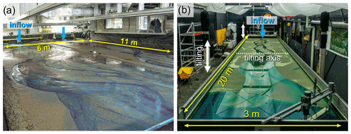
Figure 2 The flume setups of the two scale experiments tested in this study. (a) The Eurotank flume was used to simulate meandering and braided rivers in parallel on the left and right part of the flume, respectively (Van Dijk et al., 2013a). Water colour was converted to blue for visual comparison with (b) the second scale experiment in the tilting flume the Metronome that was used to simulate estuaries (Leuven et al., 2018). The flume is tilted over the short central axis, which steers flood and ebb flows that favour ample sediment transport in both tidal directions.

The tidal experiment in the Metronome flume by Leuven et al. (2018) showed the development of an entire estuary with erodible boundaries and self-formed bars on a laboratory scale. The self-formed estuary planform was characterised by along-channel alternations of shallow, wide sections that accommodated large bars and deep bottlenecks where the main confluences were found. The Metronome flume tilts over the short central axis (Fig. 2), which differs from previous stationary flume setups with sea level fluctuations (Reynolds, 1889, 1891; Mayor-Mora, 1977; Tambroni et al., 2005; Tesser et al., 2007; Stefanon et al., 2010, 2012; Vlaswinkel and Cantelli, 2011; Iwasaki et al., 2013). The tilting motion periodically generates a slope in the landward direction during flood and a slope in the seaward direction during ebb, which results in tidal currents strong enough to move sediment along the entire estuary (Kleinhans et al., 2017) (Supplement movie). The collected data constitute overhead imagery, DEMs from stereo photography and flow measurements by large-scale particle imaging velocimetry (PIV) over a tidal cycle. Earlier experiments had tidal flow driven by slow sea level fluctuations, which is closer to the cause of tidal currents in nature but leads to lower sediment mobility (e.g. Tambroni et al., 2005; Stefanon et al., 2010). Moreover, such flows can be modelled with simpler flow models (Marani et al., 2003; Stefanon et al., 2010) that provide a less rigorous test of the numerical model applied here.

3.2 Numerical model Nays2D

The numerical model Nays2D was selected to simulate water flow of fluvial and tidal landscape scale experiments for the following reasons. Firstly, Nays2D is one of few models that can account for shallow flow of maximally a few centimetres deep. This is opposed to more common models for the simulation of large-scale fluvial and tidal morphodynamics (e.g. Delft3D) that often have built-in thresholds for minimum water depths. Secondly, Nays2D is open-source (as opposed to e.g. FLOW-3D), so the technique tested in this study is freely available for third parties.

Nays2D solves the depth-averaged nonlinear shallow-water equations, given by the following three equations in Cartesian coordinates, in which Eq. (1) is the preservation of mass and Eqs. (2)–(3) are the preservation of momentum in the streamwise and transverse direction, respectively:

$$\begin{array}{}\text{(1)}& {\displaystyle \frac{\partial h}{\partial t}}+{\displaystyle \frac{\partial \left(h\stackrel{\mathrm{‾}}{u}\right)}{\partial x}}+{\displaystyle \frac{\partial \left(h\stackrel{\mathrm{‾}}{v}\right)}{\partial y}}=\mathrm{0}\text{(2)}& {\displaystyle }\begin{array}{rl}{\displaystyle \frac{\partial \stackrel{\mathrm{‾}}{u}}{\partial t}}& +\stackrel{\mathrm{‾}}{u}{\displaystyle \frac{\partial \stackrel{\mathrm{‾}}{u}}{\partial x}}+\stackrel{\mathrm{‾}}{v}{\displaystyle \frac{\partial \stackrel{\mathrm{‾}}{u}}{\partial y}}+g{\displaystyle \frac{\partial H}{\partial x}}+{\displaystyle \frac{g\stackrel{\mathrm{‾}}{u}\sqrt{{\stackrel{\mathrm{‾}}{u}}^{\mathrm{2}}+{\stackrel{\mathrm{‾}}{v}}^{\mathrm{2}}}}{C^{\mathrm{2}}h}}\\ & -{\mathit{\nu }}_t\left({\displaystyle \frac{{\partial }^{\mathrm{2}}\stackrel{\mathrm{‾}}{u}}{\partial x^{\mathrm{2}}}}+{\displaystyle \frac{{\partial }^{\mathrm{2}}\stackrel{\mathrm{‾}}{u}}{\partial y^{\mathrm{2}}}}\right)=\mathrm{0}\end{array}\text{(3)}& {\displaystyle }\begin{array}{rl}{\displaystyle \frac{\partial \stackrel{\mathrm{‾}}{v}}{\partial t}}& +\stackrel{\mathrm{‾}}{u}{\displaystyle \frac{\partial \stackrel{\mathrm{‾}}{v}}{\partial x}}+\stackrel{\mathrm{‾}}{v}{\displaystyle \frac{\partial \stackrel{\mathrm{‾}}{v}}{\partial y}}+g{\displaystyle \frac{\partial H}{\partial y}}+{\displaystyle \frac{g\stackrel{\mathrm{‾}}{v}\sqrt{{\stackrel{\mathrm{‾}}{u}}^{\mathrm{2}}+{\stackrel{\mathrm{‾}}{v}}^{\mathrm{2}}}}{C^{\mathrm{2}}h}}\\ & -{\mathit{\nu }}_t\left({\displaystyle \frac{{\partial }^{\mathrm{2}}\stackrel{\mathrm{‾}}{v}}{\partial x^{\mathrm{2}}}}+{\displaystyle \frac{{\partial }^{\mathrm{2}}\stackrel{\mathrm{‾}}{v}}{\partial y^{\mathrm{2}}}}\right)=\mathrm{0},\end{array}\end{array}$$

in which t is time (s), $\stackrel{\mathrm{‾}}{u}$ and $\stackrel{\mathrm{‾}}{v}$ are the depth-averaged flow velocity (m s⁻¹) in the streamwise (x) and transverse (y) direction, H is the water level (m), h is the water depth (m), C is the Chezy roughness (m^0.5 s⁻¹), g is the acceleration due to Earth's gravity (m s⁻²), and ν_t is the eddy viscosity coefficient (–). Eddy viscosity is approximated as

$$\begin{array}{}\text{(4)}& {\displaystyle }{\mathit{\nu }}_t={\displaystyle \frac{\mathit{\kappa }}{\mathrm{6}}}a{u}_{*}h+b\text{(5)}& {\displaystyle }{u}_{*,x}=\sqrt{{\displaystyle \frac{g\stackrel{\mathrm{‾}}{u}\sqrt{{\stackrel{\mathrm{‾}}{u}}^{\mathrm{2}}+{\stackrel{\mathrm{‾}}{v}}^{\mathrm{2}}}}{C^{\mathrm{2}}}}}\mathrm{and}{u}_{*,y}=\sqrt{{\displaystyle \frac{g\stackrel{\mathrm{‾}}{v}\sqrt{{\stackrel{\mathrm{‾}}{u}}^{\mathrm{2}}+{\stackrel{\mathrm{‾}}{v}}^{\mathrm{2}}}}{C^{\mathrm{2}}}}},\end{array}$$

in which $u_{*,x}$ and $u_{*,y}$ are the streamwise and transverse components of the shear velocity (m s⁻¹). The hydrodynamics were solved by dividing each time step into two parts, namely an advective part that was solved using a cubic-interpolated pseudoparticle (CIP) method and a nonadvective part that was solved with a conventional finite difference method (Yabe et al., 1990). Since the aim of this study is to complement bathymetric data with hydrodynamic data rather than to reproduce the experiment, sediment transport and morphological updates were disregarded.

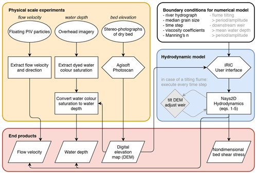
Figure 3 Workflow of integrating physical scale experiments and the numerical hydrodynamic model Nays2D to acquire water depth, flow velocity and sediment mobility maps (i.e. excluding point measurements). The DEM and corresponding boundary conditions are input to the model. Grey elements apply only to tilting flume experiments that simulate tidal systems. End products are on the bottom row and are indicators of hydrodynamics and morphological change.

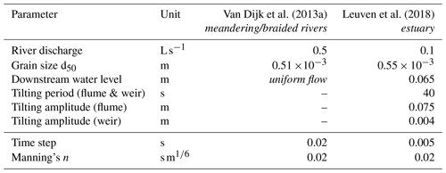
Input to Nays2D comprised a DEM of each experiment as initial condition and the corresponding boundary conditions (Fig. 3; Table 2). For the river modelling, the two DEMs (meandering and braided rivers) corresponded to the final flood stage; a constant bankfull discharge of 0.5 L s⁻¹ entered at the upstream boundary, and the water level at the downstream boundary was derived from uniform flow. For the estuary modelling, the DEM was used that corresponded to tidal cycle number 5887 (see Leuven et al., 2018), and a 0.1 L s⁻¹ river discharge entered only during the ebb phase; DEMs at later stages could not be used since the ebb-tidal delta was incomplete due to the overhanging wave generator. The estuary DEM was interpolated to a coarser rectangular grid with 2.5 cm × 2.5 cm grid cells to limit model runtime to a maximum of one day. In agreement with modelling practices for natural systems (Arcement and Schneider, 1989), a spatially uniform Manning roughness coefficient of n= 0.02 s m^1∕6 was applied, the sensitivity of which will be assessed later. The Manning roughness coefficient is described as

$$\begin{array}{}\text{(6)}& n={\displaystyle \frac{h^{\mathrm{1}/\mathrm{6}}}{C}}.\end{array}$$

The reason for not using a spatially variable friction, which could be computed from maps of grain size, is that such maps would currently include all measurement errors due to lighting and sediment colour. If these errors are significantly reduced in future studies, spatially varying friction maps are a viable option. The model was cold-started with an initial water slope equal to the valley slope of the DEM with initial flow velocities calculated from uniform flow.

Nays2D was extended to enable periodical tilting of the estuary DEM and the downstream water level boundary to drive tidal flow similar to the tilting flume the Metronome (Fig. 2). The domain was tilted sinusoidally with a period of 40 s and an amplitude of 0.075 m, meaning a maximum gradient of 0.0075 m m⁻¹. In the Metronome, the water level at the downstream boundary was set by a weir that moved in counterphase to the flume tilting so as to maintain a constant sea level of +0.065 m during tilting (see Kleinhans et al., 2017; Leuven et al., 2018, for explanation). As the experiment progressed, the weir amplitude was gradually reduced with the reduction of the length of the open sea due to the development of the large ebb-tidal delta; at tidal cycle number 5887, the weir had an amplitude of 0.004 m. To mimic the action of the weir in the model Nays2D, a sine function was imposed on the water depth at the downstream boundary, and the sea around the ebb-tidal delta was assigned a high diffusivity of b=0.02 for numerical stability.

3.3 Data analysis

Maps of water depth and flow velocity were compared to the measured data. For the two rivers, only water depth was compared, as flow velocity was not systematically measured other than sparse estimates of mid-channel flow (see Fig. S1 for modelled flow velocity maps). To explore the causes of the water depth differences between the model and the experiments, the river planforms were classified into six classes (Fig. S2). The first two classes comprised the locations of white silica flour and overhead light overexposure, which were based on the overhead imagery. The remaining four classes were morphological units with increasing levels of inundation, from a soaked bed with negligible water depth to a channel. These units were based on modelled flow, for which we used bed elevation times flow velocity to the power of 3, which proved sufficient to separate transporting channels from inactive ones (Weisscher et al., 2019).

Van Dijk et al. (2013a)Leuven et al. (2018)

Table 2 Model settings and boundary conditions of the physical scale experiments (in italics) in Nays2D. The first block of parameters is retrieved from the experiments; the second block is user-defined.

Maximum and minimum water depths in the estuary experiment were compared to bracket the tidal conditions. The 16 overhead images taken during the tidal cycle were converted into measured water depth maps. To account for incoming light from a window at the seaward side of the flume, two conversions were formulated for the upstream and downstream boundaries that were linearly interpolated along the flume. The equation for the upstream boundary was $h={\mathrm{1.43.10}}^{-\mathrm{7}}\times {\mathrm{blueness}}^{-\mathrm{15.68}}+\mathrm{0.004}$ and for the downstream boundary was $h={\mathrm{2.41.10}}^{-\mathrm{2}}\times {\mathrm{blueness}}^{-\mathrm{2.19}}+\mathrm{0.092}$, where blueness is the b^* band in the $L^{*}{a}^{*}{b}^{*}$ colour space.

Surface flow velocity measurements of the estuary experiment were compared with modelled depth-averaged velocities. To this end, the modelled flow velocities were converted to surface flow velocity using

$$\begin{array}{}\text{(7)}& u_z={\displaystyle \frac{u_{*}}{\mathit{\kappa }}}ln\left({\displaystyle \frac{z}{z_{\mathrm{0}}}}\right),\end{array}$$

in which u_z is the flow velocity (m s⁻¹) at depth z (m), with depth-averaged flow velocity at 0.36 h, and z₀ is the zero-velocity level for rough flow (m). Modelled depth-averaged flow velocity and shear velocity were used to calculate z₀, from which u_z was calculated at the water surface. Grid cells lacking one or more of the 16 PIV measurements during the tidal cycle were filtered out to enable a fair comparison of experimental data and model throughout the entire tidal cycle. The comparison focused on morphologically relevant variables; these include the tidal flow velocity maxima during the ebb and flood phases, which are important for sand transport (Friedrichs, 2011), and the tidally averaged residual flows, which are important for mud transport (Postma, 1961; Groen, 1967).

Finally, the sensitivity to the Manning roughness coefficient was tested for the range 0.016–0.024 s m^1∕6 that agrees with common coefficients for sand (Arcement and Schneider, 1989). The mean absolute error (MAE) and mean bias error (MBA) quantify the difference between the model and the measurements. The MAE is computed as the average of absolute differences between the modelled and measured data. The MBA is computed as the average difference to quantify how much the model over- or underpredicts the measured data.

4 Results

4.1 Meandering and braided rivers

4.1.1 Water depth

The modelled water depth resembles the measured data for both river types for locations where the quality of the experimental data is good (Figs. 4a–f, 5a–d, S2). Similar to the meandering river experiment, the model produces flow that is focused in a single sinuous channel, especially for x>4 m (Fig. S1), despite the multi-channel character of the DEM and the considerable overbank flow. This distinction of a main sinuous channel and swale channels is less distinct in the model for x<4 m. This is also the domain range with slightly more modelled overbank flow over the floodplain compared to the experiment (Fig. 4c). The mean absolute error is small, albeit larger for the channels (MAE =1.73 mm) than the low/high inundated areas (MAE =0.81 mm), and the model bias error is negligible (MBE $<\mathrm{0.1}\cdot$ MAE) (Fig. 5a, b), given a maximum water depth of 20 mm.

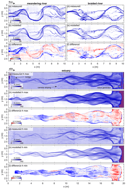
Figure 4 Measured and modelled water depth (a–c) for the meandering and (d–f) braided rivers by Van Dijk et al. (2013a) and (g–l) for the estuary by Leuven et al. (2018). In the case of the estuary, panels (g–i) show the maximum water depth during a tidal cycle, and panels (j–k) show the minimum water depth during a tidal cycle. Maps of difference are determined by subtraction of modelled from measured water depth.

The braided river model reproduces the division of flow over about two channels with little overbank flow (Fig. 4d–f). However, the model predicts slightly more water flowing through the secondary channels and less through the main channel (for example the secondary channel around x=6 m, y=1 m in Fig. 4f). Overall, the model error is slightly larger than that of the meandering river, with an MAE =2.31 mm and MBE $=-\mathrm{0.65}$ mm for channels and an MAE =1.30 mm and MBE $=-\mathrm{0.25}$ mm for low/high inundated areas (Fig. 5b, d); the bias errors indicate that modelled water depths are on average lower than the measured values for the braided river.

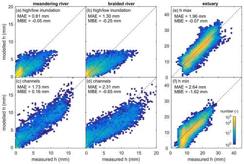
Figure 5 Comparison between measured and modelled water depths for different classes for the (a, c) meandering and (b, d) braided rivers, as well as for the (e) maximum and (f) minimum water depths in the estuary. The scatter density plots exclude floodplain and erroneous measured data (e.g. due to white silica flour), which are included in Figs. S2 (rivers) and S3 (estuary). Colours indicate the occurrence frequency.

The modelled flow is more reliable at locations with abundant white silica flour where the measured data are quite inaccurate (Figs. 1b, S2c). It is at these locations that the measured water levels, calculated as water depth from water colour added on the bathymetry, are unrealistically high above the surrounding floodplain. The reason for such large measured water depths for the upper meandering river (Fig. 4a–c) is that the white silica flour enhanced the colour contrast with respect to the yellowish sandy substrate. As a consequence, higher redness values were recorded for floured regions on the a^* band that Van Dijk et al. (2013a) used to estimate water depths. However, as this effect was unaccounted for during post-processing, unrealistically large water depths were assigned to these “redder” areas.

4.2 Estuary

4.2.1 Water depth

Periodic tilting of the estuary DEM that mimicked the motion of the tilting flume adequately reproduced the propagating behaviour of the tidal wave (Supplement movie). Moreover, the modelled tidal wave caused maximum and minimum water depths close to those observed with an MAE =1.96 mm for maximum water depths and an MAE =2.64 mm for minimum water depths (Figs. 4g–l, 5e, f, S3, S4). These errors are small compared to the largest water depths recorded in the estuary of about 35 mm.

Overprediction by the model mainly occurs at the ebb-tidal delta (x>18 m in Fig. 4i, l). This is predominantly due to the difference of the downstream boundary conditions between the experiment and the model. In particular, the amount of water entering the flume during flood was somewhat limited by the pumping capacity in the experiment. In contrast, the influx of water in the model was determined with a uniform flow assumption, causing larger inflow that increased the water depths on the ebb-tidal delta. In turn, this larger influx likely contributed to the slightly larger maximum modelled water depths especially in the downstream half of the estuary.

Underprediction by the model is primarily ascribed to two factors, namely the chosen hydraulic roughness coefficient (model-based) and the water depth conversion from colour saturation (experimental data-based). Firstly, the observations clearly show that the tidal wave propagated faster in the deeper channels than over the shallow bars, causing flow to curl around bars (Supplement movie). In the model, however, the partitioning of flow between channels and bars is less asymmetrical. As a consequence, flood-dominant channels that end in a shoal may receive more modelled inflow over their shoal during ebb, resulting in overall slightly larger water depths (e.g. the red tidal channel at x=8 m in Fig. 4l). This implies that the model diffusivity and/or hydraulic roughness on the bars are too small. Secondly, the experimental data–model comparison is sensitive to the water depth conversions, which are less accurate for shallow water depths (Figs. 5f). Specifically, the nonlinear conversion equations used in this study and by Leuven et al. (2018) overpredict water depths for very shallow flow (i.e. h<5 mm; Fig. 5f) so as to get the deeper water depths right. Therefore, measured water depths of very shallow flow over bars are too large, which explains most of the differences between model and experimental data for minimum water depths.

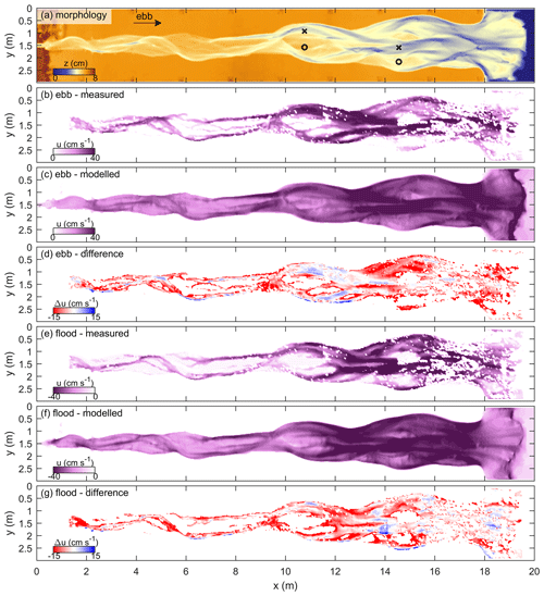
Figure 6 (b–d) Maximum ebb and (e–g) flood flow velocity with (a) the estuary morphology for reference. Maps of difference are determined by subtraction of modelled from measured surface flow velocity. “X” and “O” in (a) are the locations at which tidal stage diagrams were made in Fig. 8 of channels and shoals, respectively.

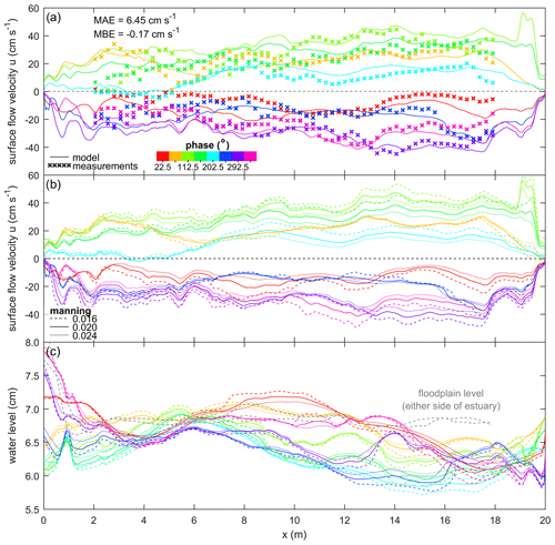
Figure 7 (a) Surface flow velocity along the estuary, given as the 90th percentile of the streamwise flow velocity component. (b) The effect of Manning on the surface flow velocity and (c) the phase-dependent median water level of each cross section along the estuary. Colours indicate the phase in the tidal cycle.

4.2.2 Ebb and flood flow

The modelled spatial pattern of peak flow velocities resembles that of the PIV measurements (Fig. 6). Both model and measurements show that peak ebb and flood flow are relatively large in channels and around bottlenecks, while they are relatively small on bars and in wider sections of the estuary. Furthermore, peak flow velocities decrease in the landward direction from ±40 cm s⁻¹ at the estuary mouth to ±30 cm s⁻¹ at x=2 m (Fig. 7a, b). Over the entire tidal cycle, the model has a small MAE =6.45 cm s⁻¹, which is about 1∕7 of the maximum surface flow velocity; in other words, the modelled order of magnitude is close to that of the measurements. Also, a different Manning roughness results in fairly similar water levels and flow velocities along the estuary, with slightly smaller flow velocities and water level variations for a higher roughness (Fig. 7b, c).

The model has full spatial cover, while experimental data are lacking particularly near the estuary mouth and for the shallower areas (Fig. 6a, b, e). Near the estuary mouth, PIV particles occasionally clumped together, which resulted in incorrect flow measurements that were excluded from comparison with the model. On the other hand, PIV measurements at shallow locations were discontinuous since the PIV particles either stranded on the bars or were drained to deeper waters. Consequently, flow velocity measurements on and around bars tend to be inaccurate, which explains the larger contrast of modelled and measured velocities for shallower areas (Figs. 6, 8). For example, the model clearly shows the wetting and drying of a tidal bar with peak flow velocities half of those in a bordering channel (Fig. 8b). The measurements in the channel are about similar but are unrealistic for the tidal bar; the PIV measurements suggest negligible flow which is incongruent with the recorded tidal water depth variations.

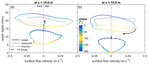
Figure 8 Tidal stage diagrams showing water depth versus surface flow velocity for a channel and shoal at (a) x=14.6 m and (b) x=10.8 m in Fig. 6a. Water depth and surface flow velocity were averaged for a 5×5 cell window. Colours indicate the phase in the tidal cycle.

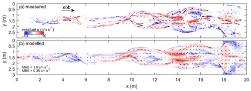
Figure 9 Residual surface flow velocity maps show similar spatial flow patterns and magnitudes between (a) the measured data and (b) model output, apart from the upstream 6 m. This upstream region was underseeded with PIV particles, which resulted in wrongly measured flow velocities. Therefore, computation of the mean absolute/bias errors was done for x>6 m.

Residual flow maps of both modelled and measured flow show the expected ebb dominance of channels and flood dominance of bars, especially at their seaward sides (Fig. 9). Also, the two circulation cells measured on the ebb-tidal delta are well-reproduced by the model. However, the overall modelled residual flow is slightly less flood-dominated (MBE is positive) than the PIV-based residual flow. For example, the flood dominance of the channel at x=14 m is weaker but still recognisable in the modelled data (Fig. 9). Further landward, a discrepancy arises in that the model suggests that the channel and bar between x=4 and 6 m are flood-dominant, while the measurements show they are mainly ebb-dominant. Inspection of the raw PIV data shows that here the flood flow is underseeded with particles, suggesting that the measured data are inaccurate and leaving the model untested in this zone.

5 Discussion

The numerical hydrodynamic model Nays2D reproduces water depths and flow velocities for physical scale experiments with both unidirectional and reversing shallow flow (Figs. 4, 6, 9). The mean absolute error of modelled water depth is within 10 % maximum water depth (Fig. 5) and of modelled flow velocity is within 15 % maximum flow velocity (Fig. 7). In other words, the errors of modelled flow fall within the range of errors that was expected in the measured data. The model results are valuable because the spatio-temporal coverage and quality of experimental data are at present more limited in typical laboratory conditions for landscape experiments. Therefore, this experimental data–model integration opens up many opportunities for the analyses of hydrodynamics in experiments in a time-efficient, cost-effective and labour-inexpensive manner. Thus far, this integration has only been used to the authors' knowledge for one set of tidal scale experiments with erodible boundaries by Tesser et al. (2007) and Stefanon et al. (2010, 2012), who numerically computed flow velocity fields by solving the Poisson boundary value problem (Marani et al., 2003). In addition to their findings, the results of this study demonstrate that an experimental data–model integration extends to complex bathymetries with unsteady, nonuniform flows.

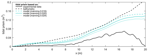
Figure 10 Tidal prism along the estuary based on experimental data, bathymetry and the model scenarios. Measured flow velocities were converted to depth-averaged velocities using Eq. (7). Tidal prism based on bathymetry (black dashed line) was computed as the cumulative volume of water along the estuary between high and low water levels imposed at the weir (i.e. with an amplitude of 4 mm) (cf. Braat et al., 2018); this calculation ignores effects of friction and river inflow.

A major advantage of numerically modelled flow fields is the full coverage and the independence from imperfect lighting, particle seeding and empirical relations through which flow properties are inferred (e.g. Van Dijk et al., 2013a; Braat et al., 2018). Additionally, the model adheres to continuity of flow, which is not the case for experimental data with errors, bias and uncertainty. Consequently, the modelled flow permits a much more accurate calculation of important flow parameters for system scaling and analysis.

One such an example is the computation of tidal prism. Tidal prism based on flow velocity and depth measurements is strongly underestimated by measurement error and missing values in shallow areas (Fig. 10). Alternatively, tidal prism could be computed using bathymetry and the cumulative volume of water between high and low water levels along the estuary, but this method ignores roughness effects and will result in an overestimation of tidal prism if the tide is a propagating wave, as opposed to a standing wave. The drawbacks of these computations are overcome by the model, which shows a steeper decrease of tidal prism in the landward direction due to roughness and a levelling-off towards the landward boundary, indicative of river inflow dominance (Fig. 10). Other important system-scale characteristics that can be derived from the modelled flow are, for example, tidal excursion length (e.g. Schramkowski et al., 2002) and the flow partitioning between multiple channels and bars (e.g. Bolla Pittaluga et al., 2003; Kleinhans et al., 2008). However, this does not mean that data need no longer be collected because the model may require calibration of, for example, hydraulic roughness.

The hydraulic roughness is commonly used to calibrate water levels and flow velocities in hydrodynamic models (e.g. Berends et al., 2019). Although a spatially constant Manning roughness of 0.02 s m^1∕6 already produced satisfying hydrodynamics, the results could be improved by calibrating a spatially varying roughness; this is especially the case for experiments with wide sediment distributions or fines (e.g. Van Dijk et al., 2013a; Braat et al., 2018). Such roughness maps could be generated from grain size maps based on overhead imagery, provided measurement errors due to lighting and sediment colour are greatly reduced. Using a spatially varying roughness may improve the partitioning of water at bifurcations over the downstream channels (for example the secondary channel in the braided river around x=6 m; Fig. 4). However, the partitioning of water over channels and bars also depends on which of the three classic assumptions of friction is applied, namely a constant Manning, Chezy or White–Colebrook roughness coefficient (Fig. 11). For example, using a constant Chezy instead of Manning would result in slightly slower flow in channels and faster flow over bars. In contrast, a constant White–Colebrook would produce faster flow in channels and slower flow over bars. In turn, these differences in flow velocity would have a considerable effect on the computed sediment mobility.

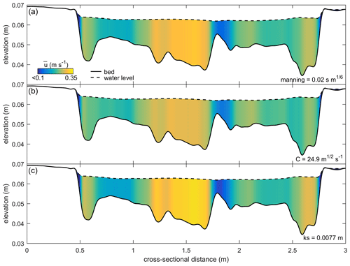
Figure 11 Effect of different hydraulic roughness predictors on the distribution of depth-averaged flow velocity $\stackrel{\mathrm{‾}}{u}$ for (a) a constant Manning, (b) a constant Chezy C and (c) a constant grain roughness k_s (White–Colebrook). The cross section is from the experimental estuary by Leuven et al. (2018) at x=15.3 m at maximum tilt in the ebb direction. Cross-sectional flow velocities were iterated for C and k_s assuming the same total discharge and water levels as modelled in this study with Manning.

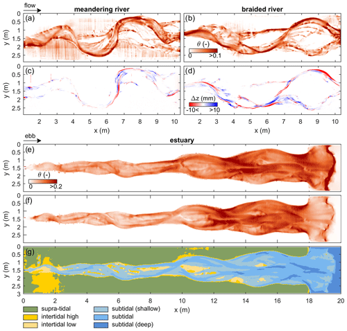
Figure 12 Complementary model data as maps of nondimensional bed shear stress (i.e. Shields numbers) and tidal zonation.  Shields numbers for the (a) meandering and (b) braided rivers with the corresponding elevation-difference DEMs (c–d) with the next time step. (e) Maximum Shields numbers for the estuary in the ebb and (f) flood direction. (g) Classification of the estuary DEM in inundation classes based on modelled tidal flow. A similar classification is also applicable to unidirectional flow in rivers, as illustrated in Fig. S2a and f.

Sediment mobility is perhaps the most important measure of flow for morphodynamics (Kleinhans and Van den Berg, 2011) (Fig. 12), but it is difficult to acquire from experiments with shallow flow. Firstly, the nondimensional mobility number allows for the comparison to natural systems (Kleinhans, 2010). Secondly, it provides vital insight into sediment transport fields and morphological activity, which is especially valuable for studying multi-channel systems and channel-bar margin interactions (De Vet et al., 2017; Van Dijk et al., 2018; Baar et al., 2019). For example, these data may be used to predict future locations of erosion and deposition (Fig. 12a–d). Also, they may be indicative of grain size or may be coupled to grain size estimations from imagery (e.g. Gardner and Ashmore, 2011).

The model is potentially applicable in conditions where data collection is hampered, such as in vegetated experiments (e.g. Braudrick et al., 2009; Tal and Paola, 2007, 2010). Application on vegetation surfaces requires the vegetation to be filtered out of the DEMs and vegetation roughness effects to be added to the model (Baptist et al., 2007; Weisscher et al., 2019). Consequently, experimental data could be enriched with water depth maps and particularly flow fields that are often absent (Table 1).

Water depth and sediment mobility maps enable unbiased classification of a river or estuary planform into inundation zones (Fig. 12g). For instance, this enables the study of the development of intertidal areas in estuaries, which are of key importance to a high biodiversity (e.g. Ysebaert et al., 2003). Moreover, such inundation classifications may effectively culminate in ecotopic maps that indicate at what locations which faunal and floral species would be likely to thrive.

Finally, the model opens up a faster way of testing the design of a flume experiment. Whilst laboratory tests need to be done in series, the model allows for testing initial and boundary conditions in parallel. Based on the resulting flow fields and bed shear stress maps at the start of the modelled flume setups (sediment transport is not included), preferred flume settings may be readily derived and applied to the physical flume. Therefore, probably fewer physical tests are required, which greatly reduces the total laboratory time. This is especially the case for experiments with different sediment mixtures and with vegetation, for which the flume needs to be emptied and cleaned after every run.

6 Conclusion

Hydrodynamic modelling with Nays2D simulates unsteady, nonuniform flows for physical scale experiments with unidirectional and reversing shallow flow. The modelling requires a DEM and the corresponding boundary conditions and produces continuous spatio-temporal data on water depth and flow velocity whilst ignoring substrate colour differences, lighting overexposure and under- or oversampling of floating PIV modules that usually decrease the quality of experimental data. Additionally, Nays2D computes sediment mobility, which is normally difficult to measure in shallow flows but is an important parameter for morphological activity and the comparison to natural systems.

The implication of this experimental data–model integration is that fewer measurements and less post-processing are required and are mainly meant for the calibration of model parameters such as the hydraulic roughness. In turn, this integration opens up many opportunities for the analyses of hydro- and morphodynamics in experiments. For example, the enhanced data enable the objective classification of the experiment planform into inundation classes which are potentially indicative of different ecotopes. Alternatively, the model allows for rigorous testing of different boundary conditions (e.g. discharge variability, sea level rise, vegetation), which could strongly reduce the time in the laboratory.