Particle size dynamics in abrading pebble populations

Abrasion of sedimentary particles in fluvial and eolian environments is widely associated with collisions encountered by the particle. Although the physics of abrasion is complex, purely geometric models recover the course of mass and shape evolution of individual particles in low- and middle-energy environments (in the absence of fragmentation) remarkably well. In this paper, we introduce the first model for the collision-driven collective mass evolution of sedimentary particles. The model utilizes results of the individual, geometric abrasion theory as a collision kernel; following techniques adopted in the statistical theory of coagulation and fragmentation, the corresponding Fokker–Planck equation is derived. Our model uncovers a startling fundamental feature of collective particle size dynamics: collisional abrasion may, depending on the energy level, either focus size distributions, thus enhancing the effects of size-selective transport, or it may act in the opposite direction by dispersing the distribution.

1 Introduction

1.1 Geological observations

Probably the most fundamental observation on pebbles is that they appear to be segregated both by size and shape, and it is broadly accepted that the dynamics are driven by two physical processes: transport and abrasion. Which of these processes dominates may depend on the geological location and also on timescales; however, geologists appear to agree that, in general, neither process should be ignored.

In coastal environments, one of the most remarkable accounts of pebble size and shape distribution is provided by Carr (1969) based on the measurement of approximately 100 000 pebbles on Chesil Beach, Dorset, England. In summarizing his results, Carr provides mean values and sample variations for maximal pebble size and pebble axis ratios along lines orthogonal to the beach. These plots reveal pronounced segregation by maximal size and shape; i.e., on shingle beaches pebbles of roughly similar maximal sizes and with roughly similar axis ratios appear to be spatially close to each other. Size and shape segregation has been broadly observed in various settings (Bird, 1996; Gleason et al., 1975; Hansom and Moore, 1981; Kuenen and Migliorini, 1950; Neate, 1967), and it was mostly attributed to the global transport of pebbles by waves (Lewis, 1931; Carr, 1969) but, in some settings, may also be related to abrasion. Indeed, a detailed account of the interaction of abrasion and transport is given by Landon (1930), who investigated the beaches on the west shore of Lake Michigan. He attributes size and shape variation to a mixture of abrasion and transport. Kuenen (1964) discusses Landon's observations but disagrees with the conclusions and attributes size and shape variation primarily to transport. Carr (1969) observes dominant sizes and shape ratios emerging as a result of abrasion and size grading, while Bluck (1967) describes beaches in South Wales where equilibrium distributions of size and shape are reached primarily by transport and abrasion plays a minor role. Which of the two processes (transport or abrasion) dominate may well depend on the timescales they operate on. While abrasion appears in some scenarios to act much more slowly than transport, a recent study (Bertoni et al., 2016) verified mass losses on the order of 50 % on a pebble beach over a 13-month period, indicating that in some settings the two processes may indeed compete in determining size and shape distributions.

In fluvial environments, while downstream fining of sediment has been often attributed to transport (Paola et al., 1992; Ferguson et al., 1996; Fedele and Paola, 2007; Whittaker et al., 2011), other authors have pointed to the significance of attrition (Brewer and Lewin, 1993; Attal and Lavé, 2006; Dingle et al., 2017). In Miller et al. (2014) the authors, using field data, provide quantitative assessment of the significance of selective transport with respect to attrition in downstream fining. Beyond the evolution of smooth size and shape distributions, there is yet another common phenomenon in fluvial geomorphology where the interaction of transport and attrition could be far from trivial. The often observed presence of isolated large boulders in rivers (Huber et al., 2020) may be explained solely by transport, as these large pieces are often not carried by the river; rather, they move by a different process (e.g., landslide or debris flow). On the other hand, these large rocks could also be interpreted as outliers emerging spontaneously in a pebble size distribution on which collisional abrasion certainly has strong impact in upper reaches of rivers.

As we can see, both in coastal and fluvial environments it is a generally accepted fact that the two processes (transport and attrition) appear to compete in shaping the evolution of pebble shape and pebble mass distributions. How exactly this competition may play out and in what manner attrition may contribute to this process is the subject of our paper.

We also remark that while all available observations indicate that attrition could be a relevant factor in the evolution of shape and mass distributions, so far, in the absence of any predictive theory, no datasets have been collected which would allow verifying any theoretical predictions. We will point out potential strategies for verification in Sect. 4.

1.2 Existing theory

1.2.1 Individual abrasion

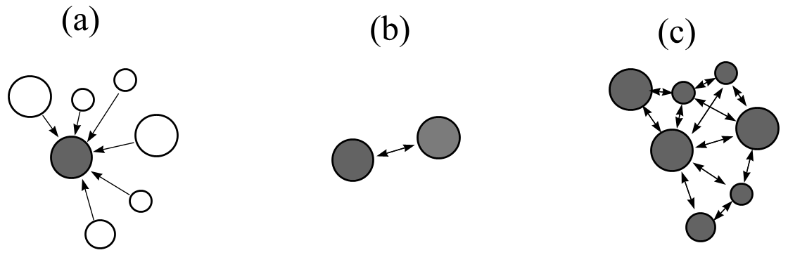
Individual abrasion is a theory describing the mass and shape evolution of one individual particle (abraded particle) under the impacts of many incoming particles (abraders) (see Fig. 1a). In the mean field theory for the geometry of individual abrasion only the mass and shape of the abraded particle is recorded; the effect of impacts is averaged and the evolution is determined by the size of the abraded particle compared to the average size of the abrading particles.

Since the seminal papers by Firey (1974) and Bloore (1977), the mean field geometric theory of individual abrasion (i.e., shape evolution) for sedimentary particles under collisions has been well understood and validated (Szabó et al., 2013, 2015; Novák-Szabó et al., 2018). Still, despite the success of the Firey–Bloore geometric theory of shape evolution, it is clear (Domokos and Gibbons, 2018) that it is not suited to predict the evolution of size: in stark contrast with geological observations summarized in Sternberg's law (Sternberg, 1875), predicting exponential decay of particle mass and an infinite lifetime for all particles, geometric abrasion theory predicted a finite lifetime for all particles. On the other hand, Sternberg's broadly accepted theory of mass evolution (Sternberg, 1875) had nothing to offer regarding the evolution of shape. Recognizing this challenge, in Domokos and Gibbons (2018) a unified theory, called volume-weighted shape evolution, has been proposed which, on one hand, reproduces all the geometric features of the Firey–Bloore geometric theory and, on the other hand, also predicts mass evolution in accordance with Sternberg's law.

1.2.2 Binary abrasion

The first stepping stone between the theory of individual abrasion and collective abrasion is the model for mutual, binary abrasion, where two particles mutually abrade each other, and we track both evolutions (see Fig. 1b). In this case one can still write mean field equations by averaging over many collisions, and the mass and shape evolution of both particles are recorded. For any binary abrasion model of size evolution, we postulate the following requirements:

• size evolution should follow Sternberg's law,

• mass loss in a collision should be a monotonically increasing function of collision energy, and

• the model should be fully compatible with the geometric evolution model.

Figure 1 Schemes for (a) individual abrasion (Firey, 1974; Bloore, 1977), (b) binary abrasion (Domokos and Gibbons, 2018), and (c) collective abrasion. Volume loss only tracked for shaded particles. Arrows represent (non-simultaneous) collision events between particles.

The unified theory in Domokos and Gibbons (2018) offers a model satisfying all three requirements: by extending the Firey–Bloore equations and Sternberg's theory and using the kinetic energy of collision, models for binary shape evolution and for binary mass evolution of two mutually abrading particles were put forward. These two models have been merged in Domokos and Gibbons (2018) into a unified volume-weighted theory of binary abrasion, compatible both with the Firey–Bloore and with the Sternberg theory. The volume-weighted model for binary mass evolution, describing the time evolutions for the masses X(t), Y(t) of two particles with respective material properties m₁, m₂ can be written as

$$\begin{array}{}\text{(1)}& {\displaystyle }& {\displaystyle }{X}_t=-c_{\mathrm{12}}{\displaystyle \frac{XY}{X+Y}},\text{(2)}& {\displaystyle }& {\displaystyle }{Y}_t=-c_{\mathrm{21}}{\displaystyle \frac{YX}{X+Y}},\end{array}$$

where the subscript t refers to differentiation with respect to time and the constant prefactors c₁₂ and c₂₁, which we call the binary abrasion parameters, depend simultaneously on the materials m₁ and m₂ of the X and Y particles, respectively.

We also note that in the case of two identical particles (e.g., two particles with identical masses X=Y and identical material properties c_XY=c_YX) the system (Eqs. 1 and 2) predicts mass evolution according to Sternberg's law. In the case of different masses or properties we still have an infinite lifetime, with one of the particles approaching zero mass asymptotically as time goes to infinity and the other particle approaching a finite mass.

1.2.3 Collective size dynamics

Independently of individual (and binary) abrasion theory there exists broad interest in collective shape and size evolution models tracking mutually colliding populations of N particles (see Fig. 1c). Similar problems arise in particular in the context of coagulation (da Costa, 2015) and dynamic fragmentation processes (Cheng and Redner, 1988). In such collective evolution models the main question is how the size distribution of particles, starting from an initial distribution, evolves in time due to the mutual collisions. These models use a standard framework relying on a so-called collision kernel. In a more general setting, the collision kernel is referred to as the interaction kernel. Our choice of terminology is motivated by the fact that in our case the only interactions are collisions.

The collision kernel can be derived from the binary equations (the physical model of the N=2 case) by incorporating statistical effects, i.e., that collision probability may depend on particle speed or mass. In Domokos and Gibbons (2018) the binary model (Eqs. 1 and 2) was extended to a kernel by introducing an additional scalar parameter r (to which we will also refer as the environmental parameter of the evolution), representing the assumption that on average, only the collision probability depends on particle size and the collision speed is independent of mass:

$$\begin{array}{}\text{(3)}& {\displaystyle }& {\displaystyle }{X}_t=-c_{\mathrm{12}}{\displaystyle \frac{X^{\mathrm{1}+r}{Y}^{\mathrm{1}-r}}{X+Y}},\text{(4)}& {\displaystyle }& {\displaystyle }{Y}_t=-c_{\mathrm{21}}{\displaystyle \frac{Y^{\mathrm{1}+r}{X}^{\mathrm{1}-r}}{X+Y}}.\end{array}$$

Note that these equations are identical to the formulas (118) and (119) in Domokos and Gibbons (2018) with α=0 in their notation and taking r=ν, X=V_X, Y=V_Y, $c_{\mathrm{12}}=c_{\mathrm{21}}=c$. Alternative interpretations of r are also possible; we will discuss the role of the environmental parameter r in detail in Sect. 2.4. Henceforth, in the main body of this paper (apart from Appendix A) we assume that the pebble population is homogeneous, i.e., that the material for all pebbles is identical so we have $c=c_{\mathrm{12}}=c_{\mathrm{21}}$ and the sole role of the constant c is to set the timescales. We will incorporate this into the time variable t, and, henceforth, for homogeneous pebble populations, we set c≡1. We will discuss the role and identification of material constants in heterogeneous pebble populations in Appendix A.

Once the kernel has been established, we make the assumption that for large N the collective size evolution is a stochastic process driven by many binary events among the particles, implying that the core of the collective process is still the abovementioned collision kernel. This allows for the construction of the master equation, also known as the Fokker–Planck equation, which describes the time evolution of the particle size distribution. Although the collective abrasion is a stochastic process, in the N→∞ limit the collision kernel will uniquely determine the global evolution of the continuous size distribution. The master equation (or Fokker–Planck equation) expresses this evolution. Determining the master equation based on the collision kernel is the second step in the statistical model.

1.3 Our model

1.3.1 Relationship to earlier models

The above-outlined structure is characteristic of coagulation fragmentation models (da Costa, 2015), in particular for non-linear fragmentation, which describe fragmentation processes triggered by binary collisions of particles. Our model may be regarded as a special case of the non-linear fragmentation models (Cheng and Redner, 1988) since, in addition to the standard framework adopted in these models, we also make two simplifying assumptions:

1. we only consider collisions where the relative mass loss is small (i.e., the particles lose only fragments with small relative mass), and

2. the small fragments generated in the collisions are not considered further in the evolution.

By implementing these two assumptions into the statistical model based on the collision kernel (Eqs. 3 and 4), we take the first step towards establishing the statistical theory of collective size and shape evolution of sedimentary particles. This approach offers multiple methodological advantages. On one hand, by using Eq. (4) as the collision kernel, our statistical model will be compatible with Sternberg's law, so we can expect the collective evolution also to observe this theory, albeit in a statistical sense. On the other hand, we can also expect all our results to be compatible with an extended (future) theory which also describes collective shape evolution based on the unified, volume-weighted geometric theory in Domokos and Gibbons (2018).

1.3.2 Basic notations

To describe our construction we will need to address both the size evolution of individual particles (under the collision kernel) as well as the evolution of size distributions. While particle size appears in both settings, we need to distinguish carefully: in individual and binary models particle size evolves in time; in collective models size distribution evolves in time. As a consequence, in the individual setting the variable denoting size may be differentiated with respect to time; in the collective setting this is not the case. We will use X, Y to denote individual particle sizes (either volume or mass) and we will use x, y to denote the independent variables of size distributions. The time evolution of individual particle size will be denoted by X(t), Y(t) with time derivatives X_t(t), Y_t(t) (arguments of a function written in subscript will refer to differentiation throughout the paper). The time evolution of size densities will be denoted by f(x,t), f(y,t) with time derivatives f_t(x,t), f_t(y,t) and size derivatives f_x(x,t), $f_y(y,t).$ We denote the expected value and variance of these size distributions, respectively, by E(t) and W(t) and we will primarily use the relative variance $R\left(t\right)=W\left(t\right)/E(t{)}^{\mathrm{2}}$ to characterize the evolution of the distributions.

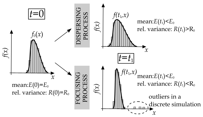
Figure 2 Schematic description of the evolution of mass distribution of a pebble population: in a dispersing process the relative size variation R(t) of the mass distribution, either represented by an empirical histogram (Carr, 1969) or a continuous function (f₀(x)) at t=0, increases. In the continuum model of a focusing process R(t) decreases as time evolves; however, in a discrete model with a finite number of particles some outliers appear (indicated by dashed ellipse) with mass substantially above the average. The reduced distribution (without the outliers) produces a decreasing relative variance, analogous to the continuous model.

1.3.3 Main results

The collision kernel (Eqs. 3 and 4) for mass evolution in Domokos and Gibbons (2018) has one single environmental parameter r, which is inherited by the corresponding Fokker–Planck equation (shown in Sect. 2.2). As we will describe in Sect. 2, the environmental parameter r may, depending on interpretation, represent either the size dependence of the number of collisions or, alternatively, the size dependence of collision energy. Regardless of the interpretation, in Sect. 2.3 we find that the value r=0.5 is critical as it separates two regimes of collective abrasion with a qualitatively different evolution R(t) of the relative variance:

• For r>0.5 we find focusing processes with decreasing R(t), approaching R(t)=0 in the limit as time approaches infinity. Here the size distribution converges to a Dirac-delta function. This parameter range corresponds to lower energy levels. Natural abrasion processes belonging to this regime will thus amplify the segregating effects of size-selective transport.

• For r<0.5 we find dispersing processes with increasing R(t), thus counteracting size-selective transport processes. This corresponds to collisional abrasion at higher energy levels.

As collisional abrasion may occur within a broad range of energies, these two basic scenarios of the model (illustrated in Fig. 2) offer an explanation for the broad range of geological observations (Bluck, 1967; Landon, 1930; Carr, 1969; Kuenen, 1964) in relating the relative significance of transport and abrasion in various scenarios. Our model also reflects the universality of Sternberg's law by predicting, regardless of the environmental parameter r, exponential decay as the universal evolution E(t) of the expected value.

In general, the evolution equations generated by Eqs. (3) and (4) for the mean E(t) and the variance W(t) are integro-differential equations which are hard to solve analytically. To support our claims, we will use three types of approximations:

• a.

  We approximate the kernel (Eqs. 3–4) by its truncated Taylor series expansion and investigate the evolution of general initial density functions. This is found in Appendix C1.

• b.

  We regard the full kernel; however, we only investigate density functions obtained as a small perturbation of the Dirac delta (i.e., populations of almost identical particles). This is done in Appendices C2 and C3.

• c.

  We numerically compute both the discrete and the continuum models. For details see Sect. 3.

We will briefly refer to the first two approximations as the continuum model. In the case of the third approximation we do direct, discrete simulations of finite particle populations; we use the full kernel and we call this the discrete model. One startling feature of the latter (as compared with the former) is the appearance of outliers, i.e., particles substantially larger than the vast majority (illustrated in Fig. 2). As we can observe, the bulk of the density function closely mimics the evolution in the continuum model. The quantitative analogy in the evolution of the relative variation R can also be recovered if we consider a reduced density function $f^{*}(t_{\mathrm{1}},x)$ by omitting the outliers, i.e., by applying an upper cutoff in size, omitting bins containing only one particle. The reduced density function $f^{*}(t_{\mathrm{1}},x)$ is characterized by the reduced relative variation R^*, which will decrease in a focusing process; however, in contrast to the continuum model, it will not approach zero but a positive constant.

1.4 Testing of the model for homogeneous pebble populations

As outlined above, our model is defined on two levels: the collision kernel (Eqs. 3–4) we will briefly refer to as the input level as it defines the basic physics of the underlying collisions. The Fokker–Planck equation we will briefly refer to as the output level as it defines the evolution of the mass density function based on the collision kernel. One may test the model at both levels. Below we discuss the case of homogeneous pebble populations where the evolution of the mass distribution is controlled by the single material parameter c and the single environmental parameter r:

• a.

  One may test the model at the input level, by fitting the kernel (Eqs. 3–4) to laboratory tests where the abrasion rate is plotted as a function of particle size. Such an experiment could be used to determine the material parameter c for a given homogeneous population. Also, if the laboratory test imitates the environment of the natural process, the environmental parameter r may also be obtained in this manner. We also note that the functional relationship between particle size and abrasion rate will not only depend on the parameters but also on particle size. For details, see Appendix A.

• b.

  One may test the model at the output level by measuring the time evolution of full mass distributions and fitting the respective material and environmental parameters c and r to this dataset. While we are not aware of any such public dataset, this could be performed in a laboratory either in a flume or in a drum experiment. In the field the optimal solution appear to be radio-tagged pebbles (Bertoni et al., 2016).

The above simple procedures apply only for homogeneous populations. We lay out the procedures for the testing of the model for heterogeneous populations in Appendix A, where we also perform partial testing for the laboratory data obtained by Attal and Lavé (2009).

2 Modeling collective size dynamics

2.1 General form of the collision kernel

The first simplification described in Sect. 1.3.1 implies that the limit where relative fragment mass approaches zero offers a good approximation; thus it permits a collision kernel of the type used in Ernst and Pagonabarraga (2007), describing continuous mass evolution via coupled ordinary differential equations for the evolution of particles with masses X(t) and Y(t):

$$\begin{array}{}\text{(5)}& {\displaystyle }& {\displaystyle }-X_t={\mathit{\psi }}^{\mathrm{1}}(X,Y),\text{(6)}& {\displaystyle }& {\displaystyle }-Y_t={\mathit{\psi }}^{\mathrm{2}}(X,Y),\end{array}$$

where ψ¹(X,Y) and ψ²(X,Y) are differentiable (C¹) functions, with positive values (i.e., ${\mathbb{R}}^{+}\times {\mathbb{R}}^{+}\to {\mathbb{R}}^{+}$). Symmetry of the binary process implies ${\mathit{\psi }}^{\mathrm{1}}(X,Y)={\mathit{\psi }}^{\mathrm{2}}(Y,X)$, so often superscripts are suppressed and the kernel is simply referred to as $\mathit{\psi }(.,.)$. Selection of the kernel encapsulates not only the physics of binary collisions, it also may include the mass-dependent probability of collision between two particles. We will discuss the identification of physically sound kernels in Sect. 2.3.

2.2 General form of the master equation

The second simplification in Sect. 1.3.1 permits the construction of the master equation solely based on the collision kernel (by omitting additional terms for the remainder of the fragmented material). These simplifying assumptions also set our model apart from general fragmentation models in another respect: in the latter, constant mass is prescribed as a global time invariant while the (integer) number of particles changes, whereas in our model total mass decreases while the number of particles remains constant and serves as a global invariant.

Using these considerations, for our problem the master equation is found to be

$$\begin{array}{}\text{(7)}& \begin{array}{rl}{f}_t(t,x)& ={\displaystyle \frac{\partial }{\partial x}}\left[f(t,x)\underset{\mathrm{0}}{\overset{\mathrm{\infty }}{\int }}f(t,y)\mathit{\psi }(x,y)\mathrm{d}y\right]\\ & =f_x(t,x)\underset{\mathrm{0}}{\overset{\mathrm{\infty }}{\int }}f(t,y)\mathit{\psi }(x,y)\mathrm{d}y\\ & +f(t,x)\underset{\mathrm{0}}{\overset{\mathrm{\infty }}{\int }}f(t,y){\mathit{\psi }}_x(x,y)\mathrm{d}y,\end{array}\end{array}$$

where subscripts stand for partial derivatives. Without loss of generality, the evolution starts at t=0 and we consider the initial distribution of the volume $f(\mathrm{0},x)\equiv f_{\mathrm{0}}\left(x\right)$ to be known a priori. Note that contrary to the majority of Fokker–Planck models, our model contains solely the advection term, which readily follows from the deterministic nature of the kernel. Here we aim to determine the collective behavior implied by Eq. (7). Nonetheless, a stochastic kernel would produce diffusion in the master equation. Such a generalization would inevitably reduce the analytic transparency and thus the qualitative predictive capability of the model. Whether or not it is justified from the quantitative point of view can be decided based on extensive testing campaigns.

We aim to understand some scenarios characteristic of pebble populations by investigating the Cauchy-type initial value problem associated with Eq. (7), starting at the distribution f₀ with mean value E₀, variance W₀, and relative variance $R_{\mathrm{0}}:=W_{\mathrm{0}}/E_{\mathrm{0}}^{\mathrm{2}}$.

2.3 Collision kernels

Detailed physical modeling of the collisional event can make the interaction kernel highly complex; for a recent review on kernels see Meyer and Deglon (2011). On the other hand, mathematical studies tend to prefer simple expressions for ψ(X,Y), permitting rigorous, analytical conclusions. Our goal is to find a kernel which has a strong physical basis yet permits an analytical approach; thus it offers a trade-off between physical and mathematical preferences.

We first consider two simple kernels which satisfy the mathematical requirement of leading to analytically soluble Fokker–Planck equations. However, as we will show, these very analytical results highlight that these kernels are physically not admissible. Next, we investigate the parameter-dependent compound kernel suggested in Domokos and Gibbons (2018), which grabs the essential physics of the investigated process, yet the corresponding Fokker–Planck equation still permits analytical conclusions.

First, we consider the summation kernel (denoted by $\mathit{\{}.{\mathit{\}}}^{+}$), where the mass loss rate is proportional to the sum of the masses of the colliding particles:

$$\begin{array}{}\text{(8)}& {\mathit{\psi }}^{+}(X,Y):=X+Y,\end{array}$$

stating that the rate of mass loss in binary collisions is proportional to the total mass of the two colliding particles. Appendix B1 demonstrates that the relative variance of the mass in the case of the summation kernel follows $R^{+}\left(t\right)=R_{\mathrm{0}}{e}^{\mathrm{2}t}$; hence it is a dispersive process regardless of the initial distribution f₀.

In the very same manner let us investigate the product kernel distinguished by the sign $\mathit{\{}.{\mathit{\}}}^{*}$. The product kernel is defined via

$$\begin{array}{}\text{(9)}& {\mathit{\psi }}^{*}(X,Y):=XY.\end{array}$$

According to Appendix B2, the relative variance in this case is constant as $R^{*}\left(t\right)=R_{\mathrm{0}}$ for all t≥0, which means that the model is neither focusing nor dispersing. Note that the time invariance of R^*(t) under the product kernel does not imply the invariance of the probability density function (PDF) f(t,x) per se. In addition, we see a polynomial decay in the mass as $E^{*}\left(t\right)=(t+E_{\mathrm{0}}^{-\mathrm{1}}{)}^{-\mathrm{1}}$, which contradicts Sternberg's law (Sternberg, 1875), which postulates an exponential decay.

In order to be in accordance with Sternberg's law and to have a control on the evolution of the relative variance, following the lead of Domokos and Gibbons (2018) we investigate the interaction law (Eqs. 3 and 4), which we call a compound kernel, and using the introduced general notation for kernels, we distinguish it with the {.}^c sign:

$$\begin{array}{}\text{(10)}& {\mathit{\psi }}^{\mathrm{c}}(X,Y):={\displaystyle \frac{X^{\mathrm{1}+r}{Y}^{\mathrm{1}-r}}{X+Y}},\end{array}$$

where $\mathrm{0}\le r\le \mathrm{1}$ is a fixed parameter. Henceforth we investigate the evolution of mass density functions under the Fokker–Planck equation derived from Eq. (10). In Appendix C1 we show analytical results for the evolution if the kernel (Eq. 10) is replaced by its truncated Taylor expansion. In Appendices C2 and C3 we show analytical results for the evolution under Eq. (10) using a Dirac delta as initial distribution. The evolution under Eq. (10) with no restrictions for the initial condition is studied numerically. The essential properties of the three investigated kernels are summarized in Fig. 3.

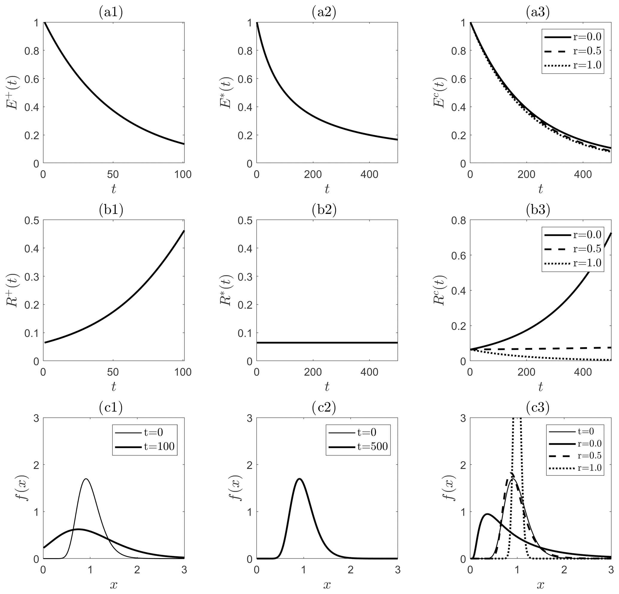
Figure 3 Evolution of an initial (t=0) lognormal probability density function under the Fokker–Planck equation generated by various kernels. Summation kernel: (a1)–(c1). Product kernel: (a2)–(c2). Compound kernel: (a3)–(c3). First row (a1–a3): mean E(t). Second row (b1–b3): relative variance R(t). Third row (c1–c3): initial (t=0) and final densities f(x,t).

2.4 Interpretation of the parameter r

In natural events, both velocity and collision probability (cross section) may depend on particle size: in laminar flows relative velocity and collision probability is proportional to linear size, while in a turbulent flows velocity could be inversely proportional to linear size and collision probability could be proportional to projected area. In the collision kernel (Eq. 10) both effects (dependence of velocity and dependence of collision probability on speed) are represented by the single scalar parameter r, so one may freely assign various interpretations to this parameter. In Domokos and Gibbons (2018) one particular interpretation was used: the compound kernel was derived using the assumption that particle velocity is independent of the size (e.g., instead determined by the surrounding fluid), but the collision probability works as a power law with particle size, i.e., X^r. The effective mass combined with the collision probability gives the kernel in Eq. (10). However, alternative interpretations are possible; the only essential underlying assumption is that we regard a one-parameter family of scenarios. In this family, if velocity is proportional to X^a and collision probability is proportional to X^b, then we have $r\simeq a+b$.

To have a global view, it may be of interest to estimate the parameter r in two extreme (limiting) scenarios. Laminar flows are characterized by a linear velocity profile. The particles hit each other if their trajectories intersect. The integration of the linear velocity profile combined with a spherical particle shape yields a collision probability proportional to $\sim X^{\mathrm{2}/\mathrm{3}}$ or, alternatively, $r\simeq \mathrm{2}/\mathrm{3}$. The other extreme case corresponds to turbulent flows, where we have equipartition; i.e., the kinetic energy of the particles is independent of their size (see, e.g., Uberoi, 1957), implying that particle velocity is proportional to $X^{-\mathrm{1}/\mathrm{2}}$. Since the area of the cross section is proportional to $X^{\mathrm{2}/\mathrm{3}}$ we arrive at a collision probability $X^{\mathrm{1}/\mathrm{6}}$ or, alternatively, $r\simeq \mathrm{1}/\mathrm{6}$. As we can see, both extreme scenarios yield r values far away to either side of the critical value $r_{\mathrm{crit}}=\mathrm{1}/\mathrm{2}$, so these estimates suggest that smooth steady conditions should result in a focusing and turbulent gas-like behavior in a dispersing process. For a detailed derivation see Appendix D.

In order to examine the validity of these assumptions we made discrete element simulations using the event-driven method (Lubachevsky, 1991). In event-driven dynamics, collisions are considered instantaneous and resolved accordingly, which is best suited to obtaining proper collision statistics. We emulated the abovementioned processes by choosing an artificial mass for the particles and simulating a chaotic system. The artificial mass was used to obtain different volume-velocity relations in different scenarios. We found that in chaotic or turbulent systems relative velocities were proportional to $v\sim X^{-\mathrm{1}/\mathrm{2}}-X^{-\mathrm{1}/\mathrm{3}}$ and the system behaved as the continuum model with $r\sim \mathrm{1}/\mathrm{6}-\mathrm{1}/\mathrm{3}$. On the other hand, if velocities were proportional to $v\sim X^{-\mathrm{1}/\mathrm{6}}-X^{\mathrm{0}}$, then the system was similar to a continuum model with $r=\mathrm{1}/\mathrm{2}-\mathrm{2}/\mathrm{3}$. Thus the discrete element simulations fully support the results of the compound kernel.

2.5 Fluvial abrasion

Here we interpret the intuitive picture of fluvial abrasion in the context of our statistical model. In our model a fluvial environment may be represented by a fluvial population, consisting of N+1 particles: a very large number (N) of small particles Xⁱ (i=1, 2, … N) representing the pebbles carried by the river and one very large particle Y representing the riverbed. Such a scenario cannot be explored directly in the context of our continuum model; however, as we will discuss in detail in Sect. 3.3, the discrete model can capture this situation even in the limit of N→∞.

To make a meaningful characterization of geologically relevant scenarios, we will regard two extreme cases which represent brackets on geological processes. In both cases we assume that the mass evolution is driven by binary collisions and we regard the limit as N, Y→∞ (while the masses Xⁱ of the small particles remain finite). Since we are interested in the mass evolution of pebbles (and in the current paper we are not interested in the mass evolution of the riverbed), we will denote the relative variance of the pebble population (i.e., all Xⁱ particles, the riverbed Y not included) by R(t). Our aim is to establish the sign of R_t(t) as the main qualitative feature of collective dynamics, as R_t(t)<0 and R_t(t)>0 imply focusing and dispersing processes, respectively.

In the first extreme scenario we assume that particles are chosen uniformly from the full fluvial population: i.e., the riverbed has no special role. In this case almost all collisions will happen among a pair of small particles (Xⁱ, X^j); thus the presence of the riverbed has no impact on the evolution of R(t). For this extreme case all predictions of our continuum model remain valid: r=0.5 will be a critical parameter value above which we see focusing (R_t<0) and below which we see dispersing (R_t>0) behavior. At the critical value r=0.5 our model predicts neutral behavior with R_t=0.

In the second extreme scenario we assume that the small particles exclusively collide with the riverbed (large particle); i.e., we only have (Xⁱ, Y)-type collisions. This means that the evolution for each of the small particles is an identical, independent two-particle process governed by the model (Eqs. 1–2) for binary collisional mass evolution. In this process, in the Y→∞ limit each individual small particle Xⁱ will thus evolve as

$$\begin{array}{}\text{(11)}& X^i\left(t\right)=X^i\left(\mathrm{0}\right)e^{-t}\end{array}$$

and thus follow Sternberg's law. It is easy to show that for any initial distribution for the masses Xⁱ(0), in this process we have R_t=0. The large Y particle (riverbed) will lose some mass as well, but in this publication we are not interested in that part of the process.

Intuitively it is clear that any geologically relevant process is in between the above two extreme cases, and, although we do not deliver a rigorous proof, it appears plausible that in a geologically relevant setting R_t will also be bounded by the two evolutions predicted for the two extreme scenarios. As for the second extreme scenario we have R_t=0; we expect that for any intermediate scenario the sign of R_t will agree with the sign of R_t based on the first extreme scenario. Our results show that the focusing behavior of the particle size distribution, or lack thereof, depends on interparticle interactions and not on the collisions between the particles and the riverbed. This would imply that all our qualitative predictions remain valid in fluvial environments.

3 Numerical results

Here we perform computations to illustrate the main results presented in Sect. 1.3.3 by discretizing time with a fixed time step Δt. The discrete model has been simulated with custom-made codes in Matlab and Python performing $M^{*}[N/\mathrm{2}]$ collisions between pairs during one time step Δt, where M is fixed model parameter and N is the size of the population. The simulation starts with the creation of N particles whose volumes are randomly sampled from the initial distribution f₀. Binary collisions are performed on uniformly selected pairs; i.e., all particles have an equal chance of being selected irrespective of their volume. Once a pair is selected, the collision kernel ψ^c is applied and the volume decrement is computed with time step $\mathrm{\Delta }t/M$. After the binary collision event both particles with a reduced volume are replaced into the sample. In the presented simulations we set the population size to be N=5000, the time step Δt=0.01, and M=10. In the continuum setting f(t,x) evolves under Eq. (7) with some initial value f₀(x). This code uses the operator exponential syntax of a the Chebfun toolbox (Driscoll et al., 2014) in Matlab.

3.1 Focusing and dispersing regimes

The evolution of a pebble population under the compound kernel was simulated both in the frame of discrete and the continuum model, i.e., by direct event-based simulation and by discretizing the partial differential equation. (see Sect. 1.3.3). The results show excellent agreement with our analytical predictions: $r=\mathrm{1}/\mathrm{2}$ does indeed appear to be a critical parameter in the model. This is illustrated in Fig. 4, where a lognormal distribution is used as an initial value for the evolution.

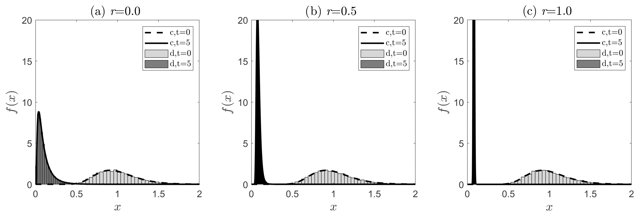
Figure 4 Evolution of a lognormal PDF in the compound kernel under the continuous (c) and discrete (d) models at the parameter values r=0.0 (a), r=0.5 (b), and r=1.0 (c) from t=0 until t=5.0. The results of the discrete simulations are given by the histograms; the output of the continuous model is given by dashed (initial distribution) and solid lines (final distribution). Observe the fair agreement between the discrete and the continuous models.

3.2 Fitted lognormal distribution

Although the lognormal distribution is certainly not invariant under the compound kernel (i.e., an initially lognormal density function does not remain lognormal in the evolution), mass distributions in later time steps highly resemble lognormal distributions. To test this visual observation we fitted lognormal distributions to the computed mass distributions in the discrete simulations. The evolution of the two parameters (respectively, denoted μ and σ) of the lognormal distribution is given in Fig. 5 at values of the parameter r. The criticality of r=0.5 is obvious in this setting, too: while the initially lognormal distribution is almost invariant under the evolution at $r=\mathrm{1}/\mathrm{2}$, the evolution of the parameters μ and σ takes an opposite direction in the parameter space for r=0.0 and r=1.0, respectively. The 95 % confidence levels of the fit confirm the visual intuition: the evolved distributions are close to lognormal: in practical applications an approximation with a lognormal distribution produces an acceptable error.

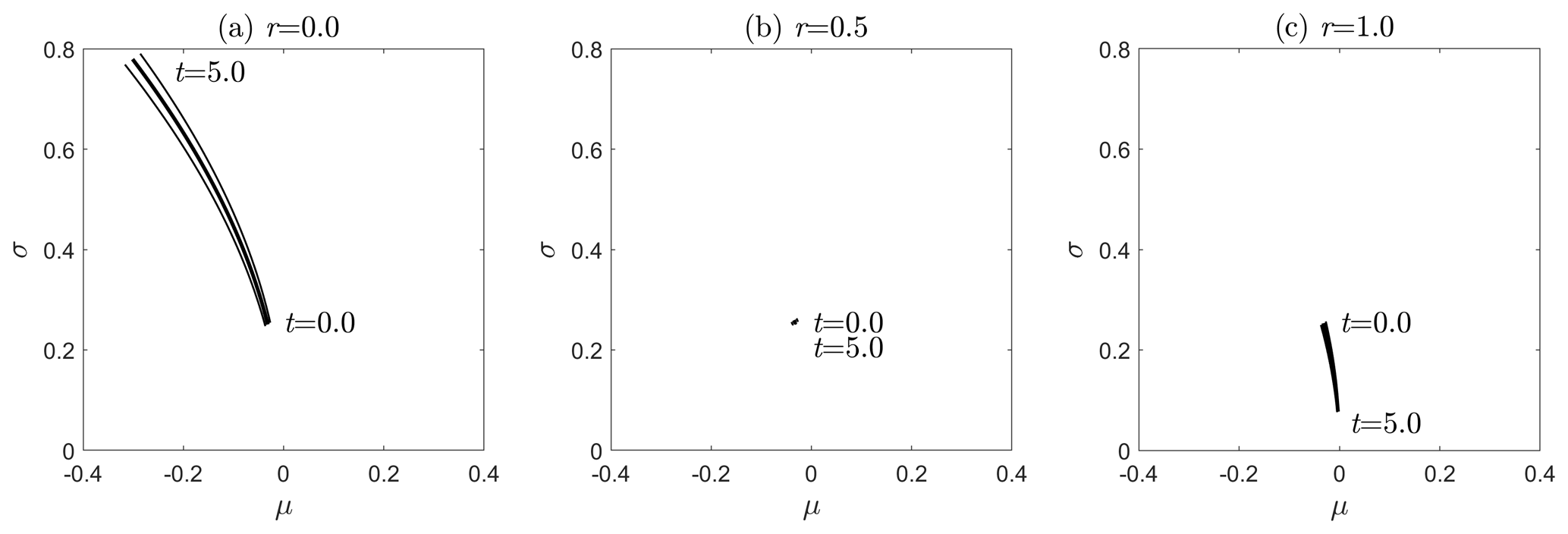
Figure 5 Parameters μ and σ of a lognormal distributions fitted to the computed mass distribution in the compound model at the parameter values r=0.0 (a), r=0.5 (b), and r=1.0 (c) from t=0 until t=5.0. Thick solid lines correspond to the best fit; thin lines indicate the 95 % confidence level of the fit. Observe the narrow zone spanned by the confidence intervals.

3.3 Outliers: anomalies in smaller samples

The continuum model describes the N→∞ limit of the system. In the computations shown in Sect. 3.1 and 3.2 we either showed results based on the continuum model or in the direct, discrete simulations we treated large (N=5000) populations. However, if we look at the discrete simulations on smaller samples we may observe unexpected phenomena not recorded in the previous computations. In Fig. 6 we show the mass distribution of a system at r=0.6 with N=2000 particles. The bulk of the histograms can be approximated well with a lognormal distribution. However, there are 12 particles with somewhat larger volume than predicted by the lognormal distribution and one approximately 150 times the median volume (5.3 times the radius). Thus inside the focusing regime we may observe a situation where we have a well-defined narrow distribution which describes the bulk of the particles, but a few might escape from this process and may be left behind, at larger mass. This effect is persistent and it was observed also for the parameter value of r≃0.7.

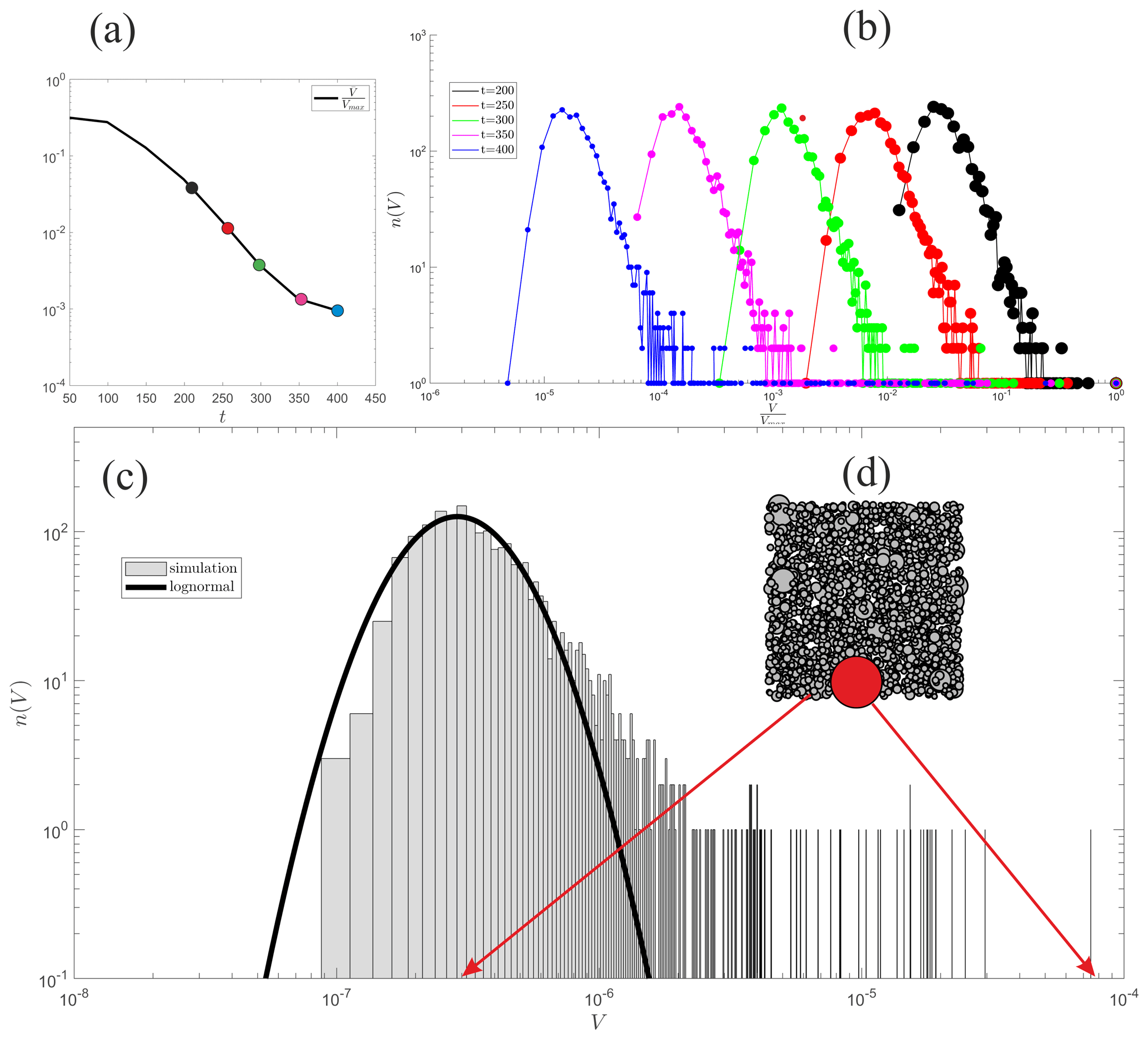
Figure 6 Simulation of a finite sample with N=2000 particles. Inset (a) shows the evolution of the mean volume normalized by the maximal volume. Inset (b) depicts the evolution of the distribution; the corresponding points in (a) are denoted by the same color. The green curve (t=300) is the one shown in detail in panel (c); it depicts the particle volume histogram after 300 collisions per particle. The gray boxes show the logarithmically binned histogram; the black line is a lognormal fit to the data. Observe the existence of outliers on the right. Inset (d) is a visual illustration of the entire population: all particles are placed randomly into a 2D container. Smaller particles were placed first and the white content (gray scale) is proportional to the linear size of the particle. One small particle close to the mean and one large particle (outlier) are marked with red and their position is indicated in the distribution.

In order to estimate the robustness of this scenario we use a simple approximation by assuming that all but one particle have volume X and one single, exceptional particle, called the “outlier”, has a volume aX with a≫1. As is demonstrated in Appendix E, the outlier can coexist with the population of the small particles. In the N→∞ limit the condition of such a coexistence reads

$$\begin{array}{}\text{(12)}& {\displaystyle \frac{\mathrm{2}{a}^r}{\mathrm{1}+a}}\le \mathrm{1}.\end{array}$$

The numerical solution of Eq. (12) for equality yields the critical curve a_crit(r) on the [r, a] parameter plane, separating systems where outliers may coexist with the population from systems where they may not. While we computed the a_crit(r) critical curve for the case of infinitely large populations (the N→∞ limit), we stress the fact that the illustrated phenomenon is inherently discrete and does not arise in the continuum model. We may explain this curious phenomenon in the following manner. Assume that we start from a narrow distribution. Then random fluctuations in the discrete system may create particles with large relative mass (i.e., a large parameter value a). If these fluctuations are sufficiently large to create particles above the critical curve a_crit(r), then these outliers will be sustained; otherwise their mass will again approach the average mass of the majority. The critical curve in Fig. 7 shows that in the vicinity of the critical value r=0.5 almost any such fluctuation will be sustained and outliers are likely to survive. However, as the parameter r increases, it becomes increasingly less likely to see sustained outliers. Another observation is that as the likelihood for the existence of outliers decreases, their expected relative size increases, which matches the common-sense observation that the larger the outlier, the less frequently it may be observed. We also note that the relationship between the collection of small particles and the large particle is essentially asymmetrical. While the evolution of the latter is strongly influenced by both the factor a and the control parameter r, the evolution of the density function for the small particles is solely controlled by the latter. In other words, adding one (or a few) very large particles to a collection of many small particles will not alter the fate of the latter, as long as the collisions between a pair of particles are based on a uniform choice.

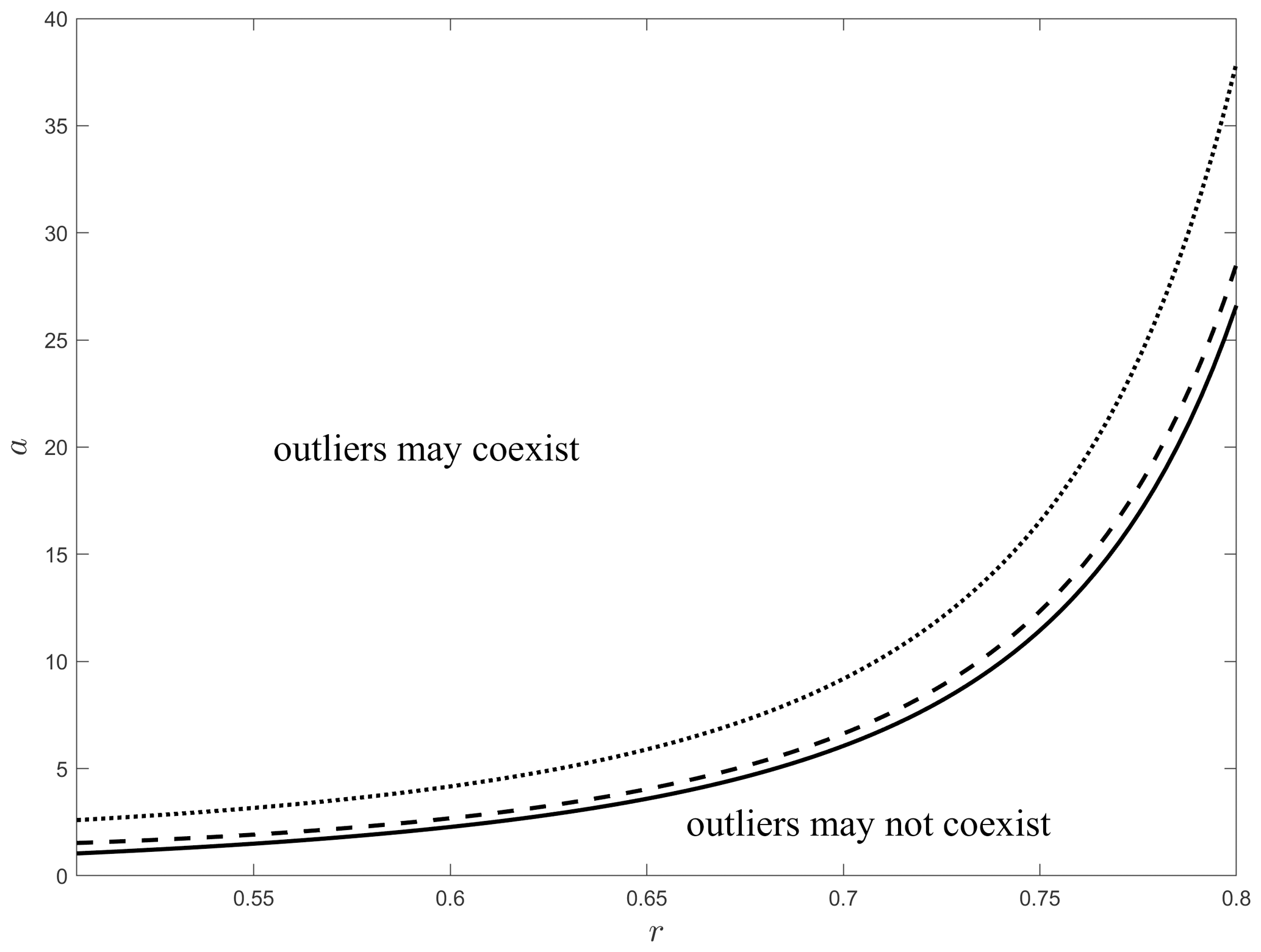
Figure 7 Critical curve a_crit(r) on the [r, a] parameter plane. Systems with parameters (r, a) associated with points above the curve permit the coexistence of outliers, while the systems associated with points below the critical curve do not permit the coexistence of outliers. The solid line belongs to the N→∞ limit, the dotted line represents N=20, and the dashed line N=100 particles.

4 Conclusions

In this paper we presented the first statistical model for the collective mass evolution of pebble populations under collisional abrasion. While our model is certainly not unique, it is compatible with

• a.

  existing geological observations,

• b.

  existing geometrical theory of individual and binary abrasion of pebbles,

• c.

  existing theory for individual mass evolution of pebbles (Sternberg's law), and

• d.

  exiting statistical theory of coagulation and fragmentation.

In the spirit of standard statistical theory for collective evolution, our model is based on two components: (i) the binary collision kernel and, based on that, (ii) the governing equation for the evolution of probability density functions for mass distribution. Regarding (i) we used the model from Domokos and Gibbons (2018), which incorporates the existing theory for individual and binary abrasion; regarding (ii) we used the Fokker–Planck equation, which is broadly used in the theory of coagulation in fragmentation.

Our collision kernel includes the single scalar parameter r which can be associated with the energy level of the collective collisional evolution process. We found that r=0.5 is critical, separating two regimes with fundamentally different behavior: for r>0.5 (low-energy regime) we found focusing behavior with decreasing relative variance R(t), and for r<0.5 (high-energy regime) we found dispersing behavior with increasing relative variance R(t). In geological terms, this result suggests that in low-energy environments collisional abrasion acts on mass distributions in unison with size-selective transport, while in high-energy environments the opposite happens and the two processes counteract each other. In accordance with prevailing geological observations and Sternberg's law, our models predicts exponential decay of particle mass in both energy regimes.

We investigated our model on two levels: (i) as a continuum model by regarding the evolution of the Fokker–Planck equation and (ii) as a discrete model by running discrete event-based simulations. In the case of the continuum model we derived our results analytically and also from numerical simulation of the Fokker–Planck equation, while in the discrete model we relied on numerical computations. With regard to the existence of the critical parameter r=0.5 and the existence of the focusing and dispersing regimes, the two approaches yielded quantitatively matching results.

Among many small pebbles, large boulders are often visible in mountain ranges or rivers. While this phenomenon is commonly attributed to transport, our model suggests that under some conditions, here again transport and abrasion may act in unison: we identified a curios phenomenon not present in the continuum model but present in the discrete model (even in the N→∞ limit). If the parameter r was in the focusing r>0.5 range but not very far from the critical value r=0.5, the bulk of the distribution narrowed (in accordance with our analytical predictions); however, we could also observe a few particles with substantially larger mass (outliers), escaping the bulk of the distribution. We characterized the mass ratio of outliers versus the mean of the bulk distribution by the parameter a, and we derived a critical curve a_crit(r) separating systems where outliers may be observed from those where this may not happen. Our result predicts that larger outliers are less likely to be observable.

While our paper only dealt with size distributions, there exist also related observations on shape: sharp peaks in distributions of axis ratios (also referred to as equilibrium shapes) are mentioned in Bluck (1967), Dobkins and Folk (1970), Landon (1930), Orford (1975), Williams and Caldwell (1988), Ashcroft (1990), Lorang and Komar (1990), Yazawa (1990), and Wald (1990). In Domokos and Gibbons (2012) a plausible argument was presented that equilibrium shapes may emerge on shingle beaches as the result of the interaction of abrasion and transport. We hope that the extension of the statistical theory presented in this paper may be capable of verifying these observations.

Appendix A: Testing the model for heterogeneous pebble populations

In the context of the binary evolution model (Eqs. 1–2) we introduced the binary abrasion parameters c₁₂ and c₂₁ and for simplicity (since we only aimed to treat homogeneous populations) we used the same notation in the collision kernel (Eqs. 3–4). Here we refine this concept in the statistical setting for heterogeneous populations where we regard the collective evolution of N particles with M≤N different materials m_i, (i=1, 2, … M). (The binary case corresponds to N=2; if the two pebbles are made from different material, then we have M=2, and for pebbles with identical materials we have M=1. In the latter case in (Eqs. 1–2) we have $c_{\mathrm{12}}=c_{\mathrm{21}}=c$.)

In the statistical setting the binary abrasion parameters can be organized into an M×M matrix M with entries c_ij, (i, j=1, 2, … M). The binary parameter c_ij is defined as the constant coefficient in the collision kernel (Eqs. 3–4) associated with the abrasion rate of particles with material m_i, bombarded by particles with material m_j. Needless to say, the matrix M is not symmetrical; in general we have c_ij≠c_ji. In particular, if material m_i is much harder than material m_j, then we expect c_ij≪c_ji.

Based on the above considerations, the statistical model is controlled by the $M\times M=M^{\mathrm{2}}$ binary abrasion parameters and the single environmental parameter r. Testing this model can be done along the strategies outlined in Sect. 1.4 for homogeneous populations; however, more detail has to be observed.

• a.

  One may test the model at the input level, by fitting the kernel (Eqs. 3–4) to laboratory tests for pair-wise selected materials m_i, m_j. In such a test the abrasion rate of particles of material m_i under abrasion from particles of material m_j is plotted as a function of particle size of the abraded particle (with material m_i). Such experiments can be used to determine the binary abrasion parameters c_ij for a given heterogeneous population. If the laboratory test imitates the environment of the natural process, the environmental parameter r may also be obtained in this manner. We will show such an example below.

• b.

  One may test the model at the output level by measuring the time evolution of full mass distributions and fitting the M² material parameters c_ij and the environmental parameter r to this dataset.

Next we show an example for testing the model at the input level by using the data obtained in Attal and Lavé (2009). Here the authors report on flume experiments where they measured the abrasion rate E_d of individual limestone gravels with a diameter between D=9 and D=39 mm mixed in approximately 400 g of 10–18 and 18–28 mm granitic gravel. In our terminology, we have M=2 (two materials) and we will use m₁ for the limestone and m₂ for the granite. The joint evolution of such a heterogeneous population is described by M²=4 binary material constants: c₁₁, c₁₂, c₂₁, and c₂₂. Attal and Lavé (2009) were primarily interested in the abrasion rates for limestone and they produced the E_d(D) plots for these particles. In this experiment we may assume that the abrasion of the limestone pebbles was exclusively due to collisions with the granitic gravel (i.e., we disregard limestone–limestone collisions). Thus the only relevant collisions are between limestone and granite, and for the mass loss X(t) of the limestone we will use Eq. (3) with X and Y denoting the volumes of the colliding limestone and granitic particles, respectively, and c₁₂ denoting the binary abrasion parameter associated with limestone being abraded by granite (not reported, but we may assume c₂₁≪c₁₂). If we replace the volume of the granitic particles by their average, the abrasion rate as function of its diameter can be calculated numerically. Note that the abrasion rate E_d in our notation reads

$$\begin{array}{}\text{(A1)}& E_d=-{\displaystyle \frac{X_t}{X}}.\end{array}$$

We fitted Eq. (3) to the dataset provided in Attal and Lavé (2009). We minimized the mean square error (with respect to the results in Attal and Lavé, 2009) for the parameters r and c₁₂ and obtained r=0.19 and c₁₂=0.28. Our fitted curves are illustrated in Fig. A1 showing fair agreement between the data and the fitted model. The value of the environmental parameter is in the range where we expect dispersing behavior, as we discussed in Appendix D, which is in accordance with the target of the original experiment which simulated abrasion in fluvial environments. We note that the same parameter pair r=0.19 and c₁₂=0.28 is valid for both limestone experiments (i.e., these parameters do not depend on the size of the particle). Our fit appears to be consistent in this respect.

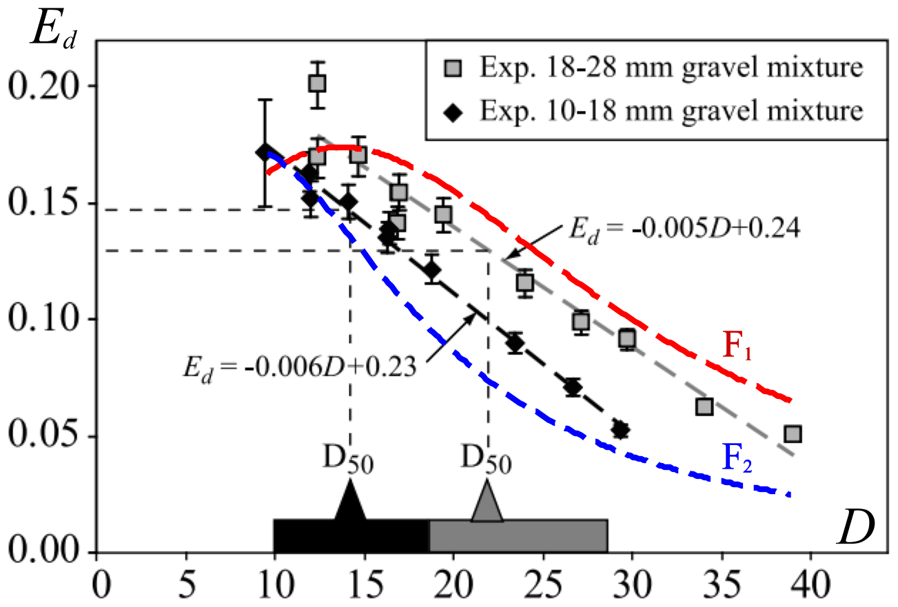
Figure A1 Abrasion rate E_d predicted by the compound kernel (Eq. 3) fitted to experimental data in Attal and Lavé (2009). Figure 9a by Attal and Lavé (2009) superposed with our model fits F₁ and F₂. Mass estimated from diameter. Least squares optimization yields r=0.19 and c₁₂=0.28.

Appendix B: Some properties of the kernels in Sect. 2.3

B1 Summation kernel

Differential equations governing the time evolution of the first and second moments can be readily obtained; hence the mean E⁺(t) and variance W⁺(t) follow the following initial value problems (IVPs):

$$\begin{array}{}\text{(B1)}& {\displaystyle }& {\displaystyle }{E}_t^{+}\left(t\right)=-\mathrm{2}{E}^{+}\left(t\right)\mathrm{with}{E}^{+}\left(\mathrm{0}\right)=E_{\mathrm{0}},\text{(B2)}& {\displaystyle }& {\displaystyle }{W}_t^{+}\left(t\right)=-\mathrm{2}{W}^{+}\left(t\right)\mathrm{with}{W}^{+}\left(\mathrm{0}\right)=W_{\mathrm{0}}.\end{array}$$

It follows that both the expectation and the variance exhibit exponential decay, namely $E^{+}\left(t\right)=E_{\mathrm{0}}{e}^{-\mathrm{2}t}$ and $W^{+}\left(t\right)=W_{\mathrm{0}}{e}^{-\mathrm{2}t}$. It is straightforward to show that the relative variance R⁺(t) increases exponentially:

$$\begin{array}{}\text{(B3)}& R^{+}\left(t\right):={\displaystyle \frac{W^{+}\left(t\right)}{E^{+}(t{)}^{\mathrm{2}}}}={\displaystyle \frac{W_{\mathrm{0}}}{E_{\mathrm{0}}^{\mathrm{2}}}}{e}^{\mathrm{2}t}=R_{\mathrm{0}}{e}^{\mathrm{2}t}.\end{array}$$

B2 Product kernel

In the case of the product kernel the IVPs describing the evolution of the mean E^*(t) and variance W^*(t), respectively, read

$$\begin{array}{}\text{(B4)}& {\displaystyle }& {\displaystyle }{E}_t^{*}\left(t\right)=-{\left(E^{*}\left(t\right)\right)}^{\mathrm{2}}\mathrm{with}{E}^{*}\left(\mathrm{0}\right)=E_{\mathrm{0}},\text{(B5)}& {\displaystyle }& {\displaystyle }{W}_t^{*}\left(t\right)=-\mathrm{2}{W}^{*}\left(t\right)E^{*}\left(t\right)\mathrm{with}{W}^{*}\left(\mathrm{0}\right)=W_{\mathrm{0}}.\end{array}$$

Here the decay of the mean and the variance are polynomial as we find

$$\begin{array}{}\text{(B6)}& \begin{array}{rl}& E^{*}\left(t\right)={\displaystyle \frac{\mathrm{1}}{t+\frac{\mathrm{1}}{E_{\mathrm{0}}}}}\mathrm{and}\\ & W^{*}\left(t\right)={{\displaystyle \frac{W_{\mathrm{0}}}{E_{\mathrm{0}}}}}^{\mathrm{2}}{\displaystyle \frac{\mathrm{1}}{{\left(t+\frac{\mathrm{1}}{E_{\mathrm{0}}}\right)}^{\mathrm{2}}}},\end{array}\end{array}$$

which result in a steady relative variance R^*(t), determined by the initial distribution f₀. Specifically

$$\begin{array}{}\text{(B7)}& R^{*}\left(t\right):={\displaystyle \frac{W^{*}\left(t\right)}{E^{*}(t{)}^{\mathrm{2}}}}={\displaystyle \frac{W_{\mathrm{0}}}{E_{\mathrm{0}}^{\mathrm{2}}}}=R_{\mathrm{0}}.\end{array}$$

Appendix C: Approximate investigation of the compound kernel

C1 Truncated compound kernel

The truncated compound kernel is obtained from the compound kernel as the truncated Taylor polynomial computed at y=x with an (O(y−x)²:

$$\begin{array}{}\text{(C1)}& {\mathit{\psi }}^{c,T}(x,y):={\displaystyle \frac{x}{\mathrm{2}}}+\left({\displaystyle \frac{\mathrm{1}}{\mathrm{4}}}-{\displaystyle \frac{r}{\mathrm{2}}}\right)(y-x)+O\left((y-x{)}^{\mathrm{2}}\right).\end{array}$$

Using the master equation, the following Cauchy problems are found that define the evolution of the mean and the variance:

$$\begin{array}{}\text{(C2)}& {\displaystyle }& {\displaystyle }{E}_t^{c,T}\left(t\right)=-{\displaystyle \frac{\mathrm{1}}{\mathrm{2}}}{E}^{c,T}\left(t\right)\mathrm{with}{E}^{c,T}\left(\mathrm{0}\right)=E_{\mathrm{0}},\text{(C3)}& {\displaystyle }& {\displaystyle }{W}_t^{c,T}\left(t\right)=-\left({\displaystyle \frac{\mathrm{1}}{\mathrm{2}}}+r\right)W^{c,T}\left(t\right)\mathrm{with}{W}^{c,T}\left(\mathrm{0}\right)=W_{\mathrm{0}}.\end{array}$$

Solution of these ordinary differential equations (ODEs) yields the evolution of the relative variance as

$$\begin{array}{}\text{(C4)}& R^{c,T}\left(t\right):={\displaystyle \frac{W^{c,T}\left(t\right)}{E^{c,T}(t{)}^{\mathrm{2}}}}={\displaystyle \frac{W_{\mathrm{0}}}{E_{\mathrm{0}}^{\mathrm{2}}}}{e}^{\left(\frac{\mathrm{1}}{\mathrm{2}}-r\right)t}.\end{array}$$

C2 A population of identical particles preserved

Here we show that a population of identical particles, characterized by a Dirac-delta function as input PDF is preserved in the model with the compound kernel regardless of the value of parameter r. Without loss of generality, we investigate the evolution from the f₀=δ(1) initial condition, where δ(x) denotes the Dirac-delta function at x. Obviously, E₀=1 and W₀=0. We show that now $f(t,x)=\mathit{\delta }\left(c\right(t\left)\right)$ holds for any t>0. Let us assume that at some $t^{*}\ge \mathrm{0}$, the distribution is $f(t^{*}*)=\mathrm{0}$. Observe that

$$\begin{array}{}\text{(C5)}& \underset{\mathrm{0}}{\overset{\mathrm{\infty }}{\int }}f\left(t^{*},y\right){\mathit{\psi }}^{\mathrm{c}}(x,y)\mathrm{d}y={\mathit{\psi }}^{\mathrm{c}}\left(x,c\left(t^{*}\right)\right).\end{array}$$

The time derivative of the mean can be computed via

$$\begin{array}{}\text{(C6)}& \begin{array}{rl}{E}_t^{\mathrm{c}}\left(t^{*}\right)& =\underset{\mathrm{0}}{\overset{\mathrm{\infty }}{\int }}{f}_t\left(t^{*},x\right)x\mathrm{d}x\\ & =-\underset{\mathrm{0}}{\overset{\mathrm{\infty }}{\int }}f\left(t^{*},x\right){\mathit{\psi }}^{\mathrm{c}}\left(x,c\left(t^{*}\right)\right)\mathrm{d}x=-{\displaystyle \frac{\mathrm{1}}{\mathrm{2}}}c\left(t^{*}\right),\end{array}\end{array}$$

where we used Eq. (7), applied integration by parts, and employed Eq. (C5). Similarly, the evolution of the variance is found to follow

$$\begin{array}{}\text{(C7)}& \begin{array}{rl}{W}_t^{\mathrm{c}}\left(t^{*}\right)& =\underset{\mathrm{0}}{\overset{\mathrm{\infty }}{\int }}{f}_t\left(t^{*},x\right)x^{\mathrm{2}}\mathrm{d}x-\mathrm{2}{E}_t^{\mathrm{c}}\left(t^{*}\right)E^{\mathrm{c}}\left(t^{*}\right)\\ & =-\mathrm{2}\underset{\mathrm{0}}{\overset{\mathrm{\infty }}{\int }}f\left(t^{*},x\right){\mathit{\psi }}^{\mathrm{c}}\left(x,c\left(t^{*}\right)\right)x\mathrm{d}x+c{\left(t^{*}\right)}^{\mathrm{2}}\\ & =-c{\left(t^{*}\right)}^{\mathrm{2}}+c{\left(t^{*}\right)}^{\mathrm{2}}=\mathrm{0}.\end{array}\end{array}$$

This shows that the variance of the distribution is constant, and it started at W₀=0; i.e., it vanishes entirely in its the evolution. In other words, we have a Dirac-delta (degenerate) distribution at any t≥0. Employing Eq. (C6) we find that the location c(t) follows the initial value problem $c_t\left(t\right)=-\frac{\mathrm{1}}{\mathrm{2}}c\left(t\right)$ with c(0)=1; hence $c\left(t\right)=\exp (-\frac{t}{\mathrm{2}})$.

C3 Dispersing and focusing behavior identified in the population of almost identical particles

As the model lacks diffusion, the behavior of a degenerate distribution with all the mass concentrated at a single value is worth studying because long-term existence of a set consisting of identical particles can take place in the model. In Appendix C2 we show that a population of identical particles remains identical in our model. In other words, the time invariance of the Dirac-delta distribution holds in our model, regardless of the value of the parameter r. Nevertheless, the value of r affects the stability of that Dirac delta: next we show that the evolution for a population of almost identical particles (i.e., a perturbed version of the Dirac-delta distribution) is either focusing or dispersing, depending on the value of r. To see this, we define a perturbed distribution. Let ε>0 be a fixed parameter and define

$$\begin{array}{}\text{(C8)}& {\widehat{f}}_{\mathrm{0}}\left(x\right):=\left\{\begin{array}{ll}(\mathrm{1}-\mathit{\epsilon })\mathit{\delta }\left(\mathrm{1}\right)+\frac{\mathrm{1}}{\mathrm{2}}& \mathrm{if}\mathrm{1}-\mathit{\epsilon }\le x\le \mathrm{1}+\mathit{\epsilon }\\ \mathrm{0}& \mathrm{otherwise}\end{array}\right..\end{array}$$

It is straightforward to show that $\underset{\mathrm{0}}{\overset{\mathrm{\infty }}{\int }}{\widehat{f}}_{\mathrm{0}}\left(y\right){\mathit{\psi }}^{\mathrm{c}}(x,y)\mathrm{d}y={\mathit{\psi }}^{\mathrm{c}}(x,\mathrm{1})$, $E_{\mathrm{0}}^{\mathrm{c}}=\mathrm{1}$, and $M_{\mathrm{2}}^{\mathrm{c}}\left(t\right):=\underset{\mathrm{0}}{\overset{\mathrm{\infty }}{\int }}f(t,x)x^{\mathrm{2}}\mathrm{d}x$ with $M_{\mathrm{2}}^{\mathrm{c}}\left(\mathrm{0}\right)=\mathrm{1}+\frac{\mathrm{1}}{\mathrm{3}}{\mathit{\epsilon }}^{\mathrm{3}}$. We aim to investigate the sign of $R_t^{\mathrm{c}}$ at t=0. Since $R^{\mathrm{c}}\left(t\right)=M_{\mathrm{2}}^{\mathrm{c}}\left(t\right)E^{\mathrm{c}}(t{)}^{-\mathrm{2}}-\mathrm{1}$, we need to study the sign of $M_{\mathrm{2},t}^{\mathrm{c}}\left(\mathrm{0}\right)E^{\mathrm{c}}\left(\mathrm{0}\right)-\mathrm{2}{E}_t^c\left(\mathrm{0}\right)M_{\mathrm{2}}^{\mathrm{c}}\left(\mathrm{0}\right)$. Integration by parts yields

$$\begin{array}{}\text{(C9)}& \begin{array}{rl}{E}^{\mathrm{c}}\left(\mathrm{0}\right)M_{\mathrm{2},t}^{\mathrm{c}}\left(\mathrm{0}\right)& -\mathrm{2}{M}_{\mathrm{2}}^{\mathrm{c}}\left(\mathrm{0}\right)E_t^{\mathrm{c}}\left(\mathrm{0}\right)=-\mathrm{2}\underset{\mathrm{0}}{\overset{\mathrm{\infty }}{\int }}{\widehat{f}}_{\mathrm{0}}\left(x\right){\mathit{\psi }}^{\mathrm{c}}(x,\mathrm{1})x\mathrm{d}x\\ & +\mathrm{2}\left(\mathrm{1}+{\displaystyle \frac{\mathrm{1}}{\mathrm{3}}}{\mathit{\epsilon }}^{\mathrm{3}}\right)\underset{\mathrm{0}}{\overset{\mathrm{\infty }}{\int }}{\widehat{f}}_{\mathrm{0}}\left(x\right){\mathit{\psi }}^{\mathrm{c}}(x,\mathrm{1})\mathrm{d}x\\ & ={\displaystyle \frac{\mathrm{1}}{\mathrm{3}}}{\mathit{\epsilon }}^{\mathrm{3}}\left({\displaystyle \frac{\mathrm{1}}{\mathrm{2}}}-r\right)+O\left({\mathit{\epsilon }}^{\mathrm{3}}\right),\end{array}\end{array}$$

where algebraic manipulations leads the last equality. In accordance with the results on the truncated model, we found that $r=\mathrm{1}/\mathrm{2}$ is critical. At $r<\mathrm{1}/\mathrm{2}$ the relative variance $R_t^{\mathrm{c}}$ is positive, it increases for any ε>0; i.e., the population of identical particles is unstable and small perturbations disperse the mass distribution. At $r>\mathrm{1}/\mathrm{2}$ the relative variance $R_t^{\mathrm{c}}<\mathrm{0}$, which shows that the population of identical particles is stable; the model is focusing.

Appendix D: Estimating physically possible values of r

In the paper we assumed that the particle collision probability depends on the volume of the particles as

$$\begin{array}{}\text{(D1)}& P\left(X\right)\propto X^r.\end{array}$$

Here we investigate two extreme scenarios, associated with the collision probabilities P_smooth(X) and P_turbulent(X) where we expect r to assume its extreme values.

The first is the smooth gradient flow. In such a case the driving fluid has a strong, but on a particle size scale constant, velocity gradient in one of the spatial directions. Such situations may arise, e.g., in shallow water layers. Here the relative velocity of the particles grows with the distance. If we are at distance u from the center of the particle in the direction of the flow velocity gradient, the collision probability P_smooth(X) can be estimated by the product of the velocity difference and the linear cross section of the particles (note that $R\equiv X^{\mathrm{1}/\mathrm{3}}$ is the linear size of the particle):

$$\begin{array}{}\text{(D2)}& P_{\mathrm{smooth}}\left(X\right)\sim {\displaystyle \frac{\mathrm{1}}{R}}\underset{\mathrm{0}}{\overset{R}{\int }}u\sqrt{R^{\mathrm{2}}-u^{\mathrm{2}}}\mathrm{d}u={\displaystyle \frac{\mathrm{1}}{\mathrm{3}}}{R}^{\mathrm{2}}={\displaystyle \frac{\mathrm{1}}{\mathrm{3}}}{X}^{\mathrm{2}/\mathrm{3}}.\end{array}$$

Based on Eq. (D1), this gives us an estimate for high $r=\mathrm{2}/\mathrm{3}$.

The other extreme case is a fully chaotic motion where equipartition takes place (Uberoi, 1957). Thus the kinetic energy of the particles ($\frac{\mathrm{1}}{\mathrm{2}}\mathit{\rho }X{v}^{\mathrm{2}}$) is independent of their volume. Thus the speed of the particles must be proportional to $X^{-\mathrm{1}/\mathrm{2}}$. If we disregard correlations, the particles have a cross section proportional to their projected area which is proportional to $X^{\mathrm{2}/\mathrm{3}}$. Combining the two gives us

$$\begin{array}{}\text{(D3)}& P_{\mathrm{turbulent}}\left(X\right)\sim X^{-\mathrm{1}/\mathrm{2}}{X}^{\mathrm{2}/\mathrm{3}}=X^{\mathrm{1}/\mathrm{6}},\end{array}$$

and based on Eq. (D1) we obtain $r=\mathrm{1}/\mathrm{6}$. Thus it is possible to have physical scenarios apparent in nature where the value of r falls to either side of the critical value of r_c=0.5 with a large enough margin.

Appendix E: Investigation of outliers in finite samples

Let us have a sample with N particles with (N−1) having the identical volume X. The last particle is an outlier with volume aX, where a≪1. In a single binary collision, a hit between particles with volume X is called an A-type event, while a collision with the outlier being involved is a B-type event. Based on discrete probabilistic considerations, the probability of an A-type event equals $(N-\mathrm{2})/N$ and a B-type event is $\mathrm{2}/N$. In the A-type event the average size $\stackrel{\mathrm{‾}}{X}$ of the particles with volume X after the collision that lasts for Δt reads

$$\begin{array}{}\text{(E1)}& \stackrel{\mathrm{‾}}{X}={\displaystyle \frac{\mathrm{2}(X-X/\mathrm{2}\mathrm{\Delta }t)+(N-\mathrm{3})X}{N-\mathrm{1}}}=X-{\displaystyle \frac{X}{N-\mathrm{1}}}\mathrm{\Delta }t.\end{array}$$

Computing $aX/\stackrel{\mathrm{‾}}{X}$ and truncating the Taylor series expansion in Δt after linear terms around the value Δt=0 yields the time derivative of the parameter a associated with an A-type event:

$$\begin{array}{}\text{(E2)}& a_t^{\mathrm{A}}={\displaystyle \frac{a}{N-\mathrm{1}}}.\end{array}$$

In the case of the B-type event both the outlier and one of the small particles follow the compound kernel via

$$\begin{array}{}\text{(E3)}& {\displaystyle }& {\displaystyle }(aX{)}_t=-{\displaystyle \frac{a^{\mathrm{1}+r}X}{\mathrm{1}+a}},\text{(E4)}& {\displaystyle }& {\displaystyle }{X}_t=-{\displaystyle \frac{a^{\mathrm{1}-r}X}{\mathrm{1}+a}}.\end{array}$$

The second equation is employed to compute the average volume of the small particles (i.e., $\stackrel{\mathrm{‾}}{X}$ associated with this event). Now we need to truncate the Taylor series of $\frac{aX-(aX{)}_t\mathrm{\Delta }t}{X-\stackrel{\mathrm{‾}}{X}}$ at Δt=0. After algebraic manipulations we find

$$\begin{array}{}\text{(E5)}& a_t^{\mathrm{B}}=-{\displaystyle \frac{a^{\mathrm{1}+r}}{\mathrm{1}+a}}+{\displaystyle \frac{a^{\mathrm{2}-r}}{(\mathrm{1}+a)(N-\mathrm{1})}}.\end{array}$$

Considering the probabilities of events A and B we arrive at

$$\begin{array}{}\text{(E6)}& a_t=a{\displaystyle \frac{N-\mathrm{2}}{N-\mathrm{1}}}-\mathrm{2}\left({\displaystyle \frac{a^{\mathrm{1}+r}}{\mathrm{1}+a}}+{\displaystyle \frac{a^{\mathrm{2}-r}}{(\mathrm{1}+a)(N-\mathrm{1})}}\right).\end{array}$$

Note that an increase in the value of a, i.e., a_t>0 implies that the outlier is getting further from the population. In the case of the N→∞ limit we find

$$\begin{array}{}\text{(E7)}& a_t=a\left(\mathrm{1}-{\displaystyle \frac{\mathrm{2}{a}^r}{\mathrm{1}+a}}\right).\end{array}$$

Here the sign of the expression in the brackets determines the sign of a_t, which coincides with Eq. (12) in the text. One can also show that if there exist a_crit>1 such that a_t=0 at a_crit, then a_t>0 for any a>a_crit. Hence, we need the a_crit>1 that makes the expression in brackets vanish. Existence of such a critical value can be shown for the case with finitely many particles, too. As we can see, sufficiently large outliers may coexist with the population in the long run. The control parameter r determines how large an outlier needs to be for sustained coexistence.