the Creative Commons Attribution 4.0 License.
the Creative Commons Attribution 4.0 License.
 | 21 Apr 2021
Effect of stress history on sediment transport and channel adjustment in graded gravel-bed rivers
Chenge An
Marwan A. Hassan
Carles Ferrer-Boix
With the increasing attention on environmental flow management for the maintenance of habitat diversity and ecosystem health of mountain gravel-bed rivers, much interest has been paid to how inter-flood low flow can affect gravel-bed river morphodynamics during subsequent flood events. Previous research has found that antecedent conditioning flow can lead to an increase in critical shear stress and a reduction in sediment transport rate during a subsequent flood. However, how long this effect can last during the flood event has not been fully discussed. In this paper, a series of flume experiments with various durations of conditioning flow are presented to study this problem. Results show that channel morphology adjusts significantly within the first 15 min of the conditioning flow but becomes rather stable during the remainder of the conditioning flow. The implementation of conditioning flow can indeed lead to a reduction of sediment transport rate during the subsequent hydrograph, but such an effect is limited to within a relatively short time at the beginning of the hydrograph. This indicates that bed reorganization during the conditioning phase, which induces the stress history effect, is likely to be erased with increasing intensity of flow and sediment transport during the subsequent flood event.
- Article
(8580 KB) - Full-text XML
-
Supplement
(703 KB) - BibTeX
- EndNote


Prediction of sediment transport is of vital importance because it is related to many aspects of river dynamics and management, including river morphodynamics modeling (Parker, 2004), river restoration (Chin et al., 2009), aquatic habitats (Montgomery et al., 1996), natural hazard planning (Marston, 2008), bedrock erosion (Sklar and Dietrich, 2004), and landscape evolution (Howard, 1994). In gravel-bed rivers, sediment transport is controlled by flow magnitude and flashiness, sediment supply, bed surface structures, channel morphology, and the grain size distribution (GSD) of sediment (Montgomery and Buffington, 1997; Masteller et al., 2019). Therefore, prediction of sediment transport in mountain rivers still remains difficult despite the large body of existing theories. This is due to the fact that these theories were mostly developed for lowland streams with continuous sediment supply and an average flow regime, which do not apply to mountain streams (Gomez and Church, 1989; Rickenmann, 2001; Schneider et al., 2015).
For example, the hydrograph of mountain gravel-bed rivers is often characterized by large fluctuations of flow discharge, including both short-term flash flood and long-term inter-flood low flow (Powell et al., 1999). However, research on the morphodynamics of mountain rivers often focuses on the effects of floods (or constant high flow) and neglects the role of inter-flood low flow, with the consideration that most sediment transport and morphological adjustments of mountain rivers occur during relatively high flows (Klingeman and Emmett, 1982; Paola et al., 1992).
Reid and colleagues (Reid and Frostick, 1984; Reid et al., 1985) studied the effects of inter-flood low flow on subsequent sediment transport in Turkey Brook, England. They found that bed load transport rates were reduced during relatively isolated flood events (e.g., events separated by long time intervals) compared to those that were closely spaced, with the entrainment threshold up to as large as 3 times higher. They linked this with sediment reorganization during prolonged periods of antecedent flow, which can make the river bed more armored and more resistant to entrainment, thus delaying the onset of sediment mobility in the following flood event. Carling et al. (1992) also reported differences in the initial motion criteria between flood events due to changes in packing and orientation of sediment particles.
To further study such “memory” effects of antecedent flow on the sediment transport during a subsequent flood, a number of flume experiments and field surveys have been conducted in the past decade, and different terms have been proposed, including “stress history effect” (Monteith and Pender, 2005; Paphitis and Collins, 2005; Haynes and Pender, 2007; Ockelford and Haynes, 2013), “flood history effect” (Mao, 2018), and “flow history” (Masteller et al., 2019). The difference in the terminology could be partly due to the available data and the chosen approach in different research works. Here we adopt the term “stress history”. It should also be noted that the approach based on shear stress (and therefore terminology), even though widely applied for laboratory experiments, is much less reliable for field measurements.
Paphitis and Collins (2005) conducted flume experiments to study the entrainment threshold of uniform sediment subjected to antecedent flow durations of up to 120 min. They found that with a longer and higher antecedent flow, the critical bed shear stress increases and the total bed load flux decreases. The work of Paphitis and Collins (2005) was extended by Monteith and Pender (2005) and Haynes and Pender (2007) to consider bimodal sand–gravel mixtures. They found that for a graded bed, longer periods of antecedent flow increase bed stability due to local particle rearrangement, in agreement with Paphitis and Collins (2005), whereas higher magnitudes of antecedent flow reduce bed stability due to selective entrainment of the fine matrix on bed surface, counter to Paphitis and Collins' (2005) conclusion based on uniform sediment. Haynes and Pender (2007) further analyzed the two competing effects and concluded that particle rearrangement may be of greater relative importance than the winnowing of the fine sediment, as it affects subsequent sediment transport. By using high-resolution laser scanning and statistical analysis of the bed topography, Ockelford and Haynes (2013) also demonstrated that the response of bed topography to stress history is grade-specific: bed roughness decreased in uniform beds but increased in graded beds with an increase length of an antecedent flow period. Performing a series of flume experiments, Masteller and Finnegan (2017) studied the evolution of the river bed on particle scale during low flow. They linked reduction of bed load flux to the re-organization of the highest protruding grains (1 %–5 % of the entire bed) on the bed surface.
Because of the above-mentioned research, existing sediment transport formulae for gravel-bed rivers (e.g., Meyer-Peter and Müller, 1948; Parker, 1990; Wilcock and Crowe, 2003; Wong and Parker, 2006) are regarded as inaccurate because they do not take the effect of stress history into account. To this end, Paphitis and Collins (2005) proposed an empirical formula for the exposure correction factor in the critical shear velocity for a uniform sand-sized bed based on their experimental data. Johnson (2016) developed a state function for the critical shear stress in terms of transport disequilibrium, which incorporates the effects of stress history and hydrograph variability. Ockelford et al. (2019) proposed two forms of functions to link the antecedent duration and the critical shear stress. The two alternatives proposed by Ockelford et al. (2019) correct the function proposed by Paphitis and Collins (2005), whose exposure correction uses a logarithmic function that implicitly assumes an unbound growth as antecedent time tends towards infinity.
Research to date has shown that antecedent flow can stabilize the river bed, thus influencing the threshold of sediment motion and bed load flux. However, most of the previous research about stress history is either under conditions with relatively low sediment transport or with relatively short durations of sediment transport in order to capture the threshold of sediment motion (Monteith and Pender, 2005; Paphitis and Collins, 2005; Haynes and Pender, 2007; Ockelford and Haynes, 2013; Masteller and Finnegan, 2017; Ockelford et al., 2019). On the other hand, other researchers have found that exceptionally high-discharge events can reduce critical shear stress by disrupting particle interlocking and breaking of bed structure (Lenzi, 2001; Turowski et al., 2009, 2011; Yager et al., 2012; Ferrer-Boix and Hassan, 2015; Masteller et al., 2019). Flume experiments by Masteller and Finnegan (2017) also indicate an increase in the number of highly mobile, highly protruding grains in response to sediment-transporting flows. Therefore, the effect of high-discharge events in reducing the critical shear stress likely counterbalances the stress history effect of antecedent flow to increase the critical shear stress. Besides, the supply of fine sediment (during high-discharge events) is also widely observed to enhance the mobilization of coarse sediment (Wilcock et al., 2001; Curran and Wilcock, 2005; Venditti et al., 2010). In consideration of these opposing mechanisms, how long the stress history effect can last during a subsequent flood event is not well understood. Such a question is important especially in light of the fact that most sediment transport and channel adjustment of mountain gravel-bed rivers occurs during high-discharge events, when the flow shear stress is high.
In this paper, flume experiments consisting of high and low flow are conducted to study this problem. The experimental arrangement is described in Sect. 2. In Sect. 3, we present the experimental results showing how channel morphology and sediment transport during a subsequent hydrograph respond to various durations of antecedent conditioning flow. The threshold of motion is analyzed in Sect. 4 based on the experimental data. Implications and limitations of this study are also discussed in Sect. 4. Finally, conclusions are summarized in Sect. 5.
The experimental arrangements were guided by conditions observed in East Creek, a small mountain creek in Malcolm Knob Forest, University of British Columbia (for details on the study site, see Papangelakis and Hassan, 2016). To investigate the study objectives, we conducted flume experiments in the Mountain Channel Hydraulic Experimental Laboratory at the University of British Columbia. The experiments were conducted in a tilting flume with a length of 5 m, a width of 0.55 m, and a depth of 0.80 m. The initial slope was 0.04 m/m. Water (but not sediment) was recirculated by an axial pump. A set of six experiments (REF2–REF7) was conducted; the experimental conditions are briefly summarized in Table 1. For experiments REF3–REF7, the same hydrograph and sedimentograph were conducted but with different durations of constant conditioning flow prior to the hydrograph or sedimentograph. It should be noted that in the experiments we only implemented the rising limb of the hydrograph or sedimentograph, rather than a full hydrograph or sedimentograph with both rising and falling limbs. Rather than studying river adjustment during a flow hydrograph, we aimed at determining the influence of conditioning time on bed load and bed surface arrangements as flow rates increased. We denote these as REF3 (10), REF4 (2), REF5 (5), REF6 (15), and REF7 (0.25), with the numbers in the brackets denoting the duration of the conditioning flow in hours. Experiment REF2 (15) consists of a 15 h conditioning period without a subsequent hydrograph or sedimentograph to test the reproducibility of our experimental results during the conditioning flow.
Table 1Summary of the experimental conditions and measurements. The experiments are listed in the table in order of decreasing duration of conditioning flow.
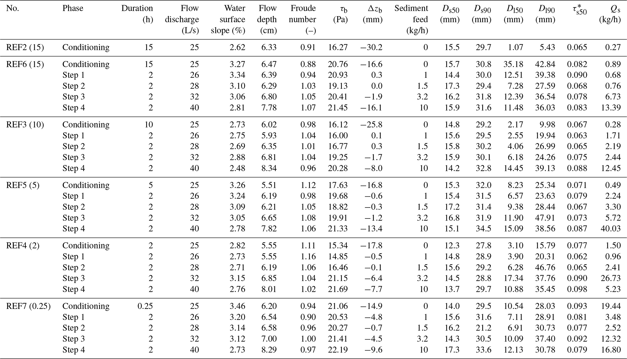
Qs: bed load transport rate; Δzb: mean difference of bed elevation averaged over the whole river channel; τb: shear stress; Ds50 and Ds90: D50 and D90 of bed surface; Dl50 and Dl90: D50 and D90 of bed load; : Shields number for Ds50. Here D90 denotes the grain size such that 90 % is finer, and D50 denotes the grain size such that 50 % is finer. All values presented in this table are measured at the end of each stage, except for Δzb, which denotes the mean difference of bed elevation during each stage (i.e., difference between the end of this stage and the end of last stage). A positive value of Δzb denotes aggradation, and a negative value of Δzb denotes degradation.
Figure 1 shows the water and sediment supply implemented during the experiments. The water discharge was selected to represent typical flows in East Creek, with the 25 L/s flow during the conditioning period being equivalent to half the bankfull flow, and the peak flow discharge of 40 L/s during the hydrograph being about 1.1 times the bankfull flow in East Creek. Because the purpose of this paper is to study the evolution of bed stability, sediment was not fed during the conditioning flow. For each step of the hydrograph, the feed rate of sediment was specified to be close to the transport capacity of the flow. Determination of the sediment supply rates was facilitated by a numerical model, which was calibrated for similar experimental conditions (Ferrer-Boix and Hassan, 2014). Sediment was fed into the flume at the upstream end using a conveyor belt feeder at the calculated transport rate capacity. The feed rate of the sedimentograph ranged between 1 and 10 kg/h. Both the hydrograph and the sedimentograph consisted of four steps, with each step lasting for 2 h.
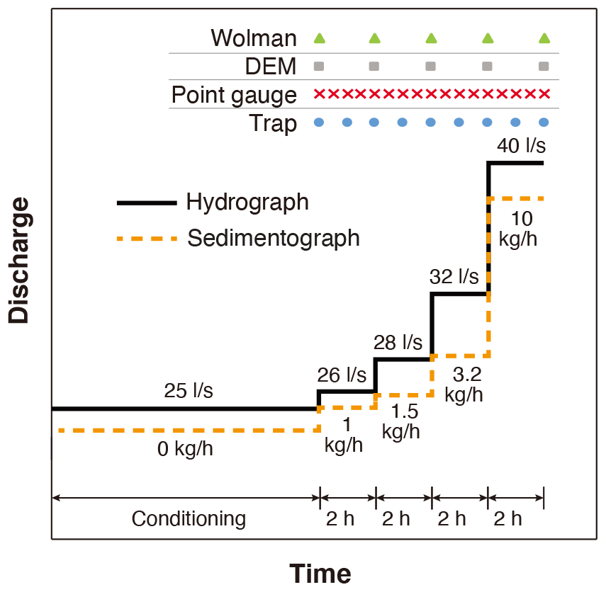
Figure 1Water and sediment supply implemented in the experiments. Markers at the top of the figure denote the time of measurements during the hydrograph phase. The time of the measurements during the conditioning phase is not shown in this figure.
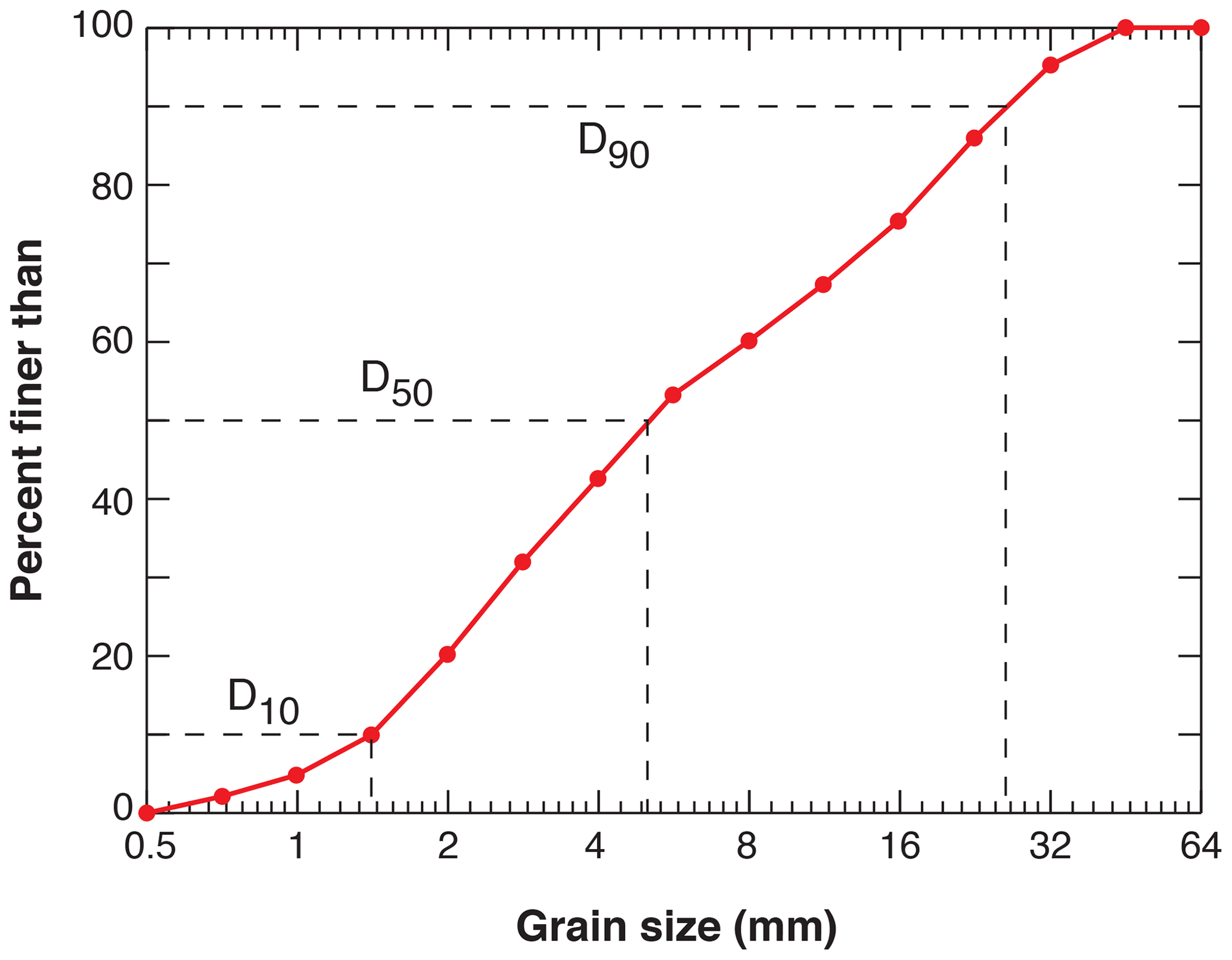
Figure 2 shows the GSD of the bulk sediment used in the experiments, with the grain size ranging between 0.5 and 64 mm. The GSD was scaled from East Creek by a ratio of 1:4, except that sediment (after scaling) with a grain size less than 0.5 mm was excluded. This preserved the entire gravel distribution of East Creek with a maximum size of 256 mm (scaled to 64 mm in Fig. 2). The model was “generic” rather than specific. This means that no attempt was made to reproduce the geometric details of the prototype channel. The bulk sediment was sieved at half φ intervals, and each grain size class was painted in different colors for texture analysis and visual identification. Before the commencement of each experiment, we hand-mixed and leveled the bulk sediment to make a flat and uniform layer of loose material with a depth of 0.15 m. The sediment was then slowly flooded and then drained to aid settlement. The bulk sediment was also used for the sediment feed in each experiment.
The bed and water surface elevations were measured along the flume every 0.25 m using a mechanical point gauge with a precision of ±0.001 m. Water depth fluctuations due to wave effects at a point were about 5 % or less. Water surface slope and bed slope are calculated based on a linear regression of the point gauge data measured between 0.5 and 4.75 m upstream of the outlet. The most upstream and downstream sections are excluded to avoid boundary effects. A green laser scanner mounted on a motorized cart was also used to measure the bed surface elevation along the flume. Bed laser scans were composed of cross sections spaced 2 mm apart with 1 mm vertical and horizontal accuracy (for details, see Elgueta-Astaburuaga and Hassan, 2017). The standard deviation of bed elevation was calculated based on the digital elevation model (DEM) data from scans. Before the calculation of standard deviation, the DEM was detrended based on linear regression to remove spatial trends with scales larger than the scale of sediment patterns (e.g., bed slope or undulations). To estimate the particle size distribution of the bed surface we used digital cameras mounted on a motorized cart along the entire flume. Images were merged together to visualize the bed and perform the particle size analysis (Chartrand et al., 2018). To avoid distortion effects due to image merging, the width of the image strips that were stitched to get a composite image was specified as just 2 cm. The particle size distribution of the bed surface was estimated using the Wolman (point count) method by identifying the grain size of particles at the intersections of a 5 cm grid superimposed on the photograph. Individual grains were identified by color. For each experiment, the grain size distribution of the bed surface was calculated at different times to quantify its changes during the experiment.
The sediment transport rates for various size ranges were measured at the end of the flume using a light table (for details, see Zimmerman et al., 2008; Elgueta-Astaburuaga and Hassan, 2017) and automated image analysis at a resolution of 1 s. Material evacuated from the flume was trapped in a 0.25 mm mesh screen in the tailbox, weighted and sieved at half φ intervals, and then used to calibrate the light table data. To avoid random fluctuations in sediment transport, we report the bed load transport rate measured by light table at a 5 min resolution and characteristic grain sizes of bed load at 15 min resolution. A range of methods for the estimation of bed shear stress has been suggested in the literature (reviewed in Whiting and Dietrich, 1990). In this study, the shear stress is estimated using the depth–slope product corresponding to normal (steady and uniform) flow. This method is selected because the focus of this work is on overall (mean) parameters controlling bed evolution; in addition, the water was too shallow to use an ADV. The water surface slope, rather than bed slope, is implemented in the calculation of shear stress, with the consideration that water surface slope is closer to the friction slope and also has less random fluctuations than bed slope.
The frequency of measurements during the hydrograph phase is also plotted in Fig. 1a, with the point gauge measurements conducted every 30 min, the trap weighting and sampling conducted every hour, and the DEM and Wolman measurements by laser scan and photograph conducted every 2 h (i.e., at the beginning and end of each stage of the hydrograph). For each measurement of DEM and Wolman, we stopped the pump instantaneously and let the flow slowly lower and then stop to allow for the bed to be scanned by a laser and photographed. The time interval between the stop of the pump and the stop of the flow was about 3 to 4 min. To avoid the influence of the following rising discharge, all subsequent measurements were taken after the flow became stable. The frequency of measurement during the conditioning phase was adjusted in each experiment in accordance with the duration of the conditioning phase and is therefore not plotted in Fig. 1.
The uncertainties associated with the measurement are also studied. For the uncertainties of the standard deviation of bed elevation, we scanned the floor of the flume twice and calculated the standard deviations of the scanned DEM. The floor of the flume was horizontal and flat, with no sediment on the bed. Theoretically, the standard deviation of the DEM should be zero. Therefore, the calculated standard deviations of the flume floor are regarded as an estimation of the uncertainties of our calculations during the experiment. To estimate the uncertainties of the bed surface GSD, for each measurement the Wolman method was implemented five times on the same photograph, with 100 samples or counts each time. The five measured GSDs for each time interval were used to calculate the mean and standard deviation of the bed surface texture (in terms of Ds10, Ds50, and Ds90). To estimate the uncertainties of the light table method, we compare the data measured by the light table with the data measured by the sediment trap, in terms of both sediment transport rate and the characteristic grain sizes of sediment load. To estimate the variations of the measured and calculated data, we calculate their coefficient of variation (cv), defined as the ratio of the standard deviation to the mean value.
Table 1 presents an overall schematization of the experimental results, including water surface slope, flow depth h, Froude number Fr (), where u is depth-averaged flow velocity), bed load transport rate Qs, shear stress τb, D50 and D90 of bed surface (Ds50 and Ds90), D50 and D90 of bed load (Dl50 and Dl90), and Shields number for a given Ds50. D90 denotes the grain size such that 90 % is finer, and D50 denotes the grain size such that 50 % is finer.
3.1 Channel adjustment
In this section, we present the channel adjustments during each experiment. Figure 3 shows the difference of longitudinal DEM averaged over the cross section, which can represent the adjustment of channel topography during different periods of the experiment. The DEM averaged over the cross section is used here to study the overall aggradation or degradation of the channel. For reference, detailed information about the DEM at different times during the experiment is provided in the Supplement, with REF6 (15) as an example. From Fig. 3a we can see that, for each experiment, evident degradation occurs during the first 15 min, especially at the upstream end of the flume. This is due to the fact that no sediment supply is implemented during the conditioning period and the initial bed material is relatively loose. From 15 min until the end of the conditioning phase (as shown in Fig. 3b), no evident aggradation or degradation is observed for any experiment, indicating that most of the adjustment of channel topography during the conditioning phase has been accomplished within the first 15 min. For step 1 of the hydrograph (as shown in Fig. 3c), no evident aggradation or degradation is observed for any of the experiments (with the mean difference of bed elevation Δzb less than ±1 mm, as shown in Table 1), except for REF7 (0.25), which has the shortest conditioning phase and experienced a mean degradation of 4.8 mm over the whole bed channel. Similarly, the channel remains relatively stable during step 2 of the hydrograph for all experiments (as shown in Fig. 3d), with no evident aggradation or degradation being observed (the mean difference of bed elevation Δzb is less than ±1 mm for all experiments). With the increase of flow discharge, some degradation (with a magnitude of about 10–20 mm) can be observed in step 3 for all experiments at the upstream end of the channel, as shown in Fig. 3e. Such degradation becomes more evident over the entire channel in step 4 of the hydrograph, when flow discharge reaches its peak value. This is in agreement with the values of Δzb presented in Table 1.
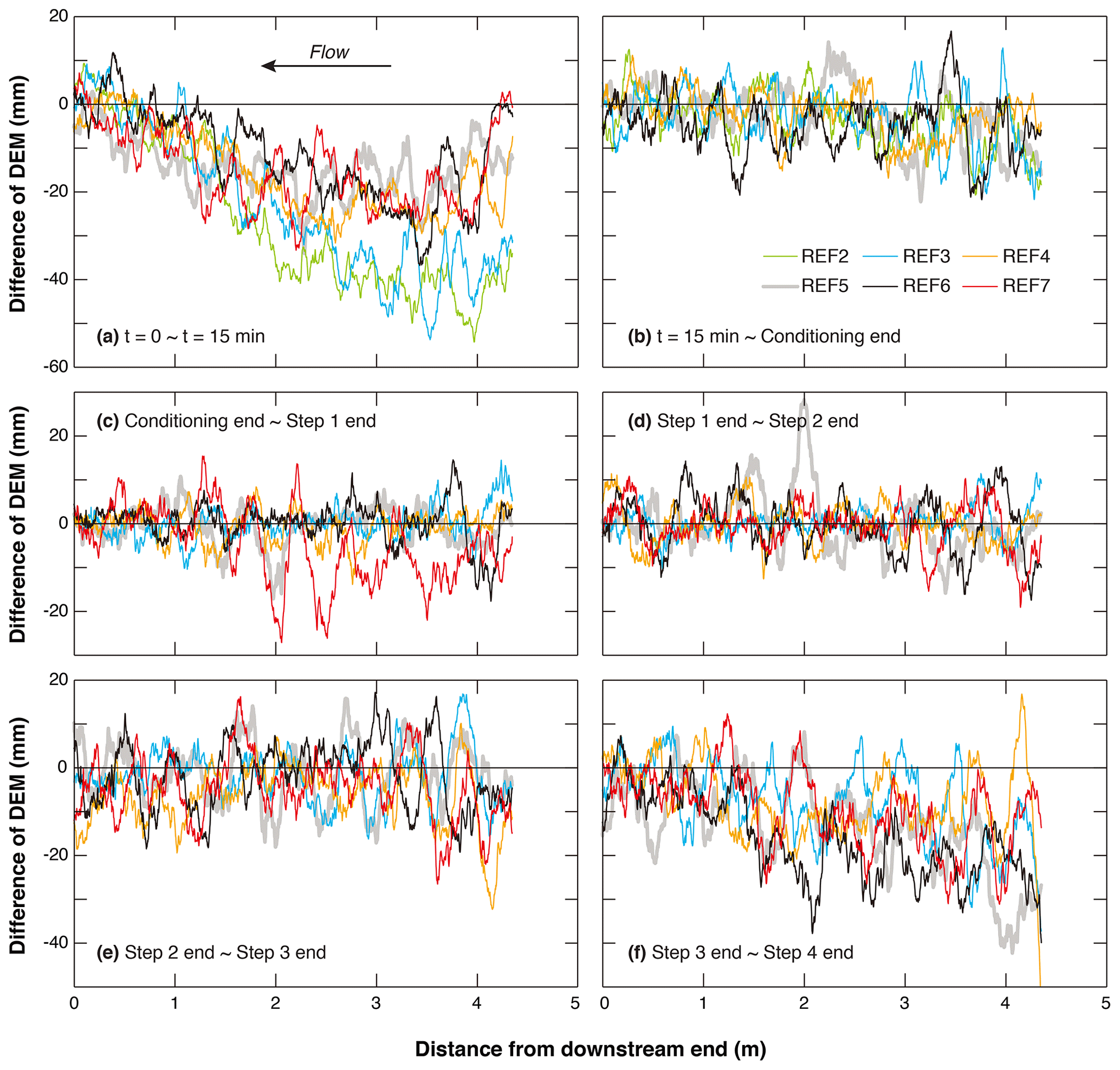
Figure 3Spatial distribution of elevation difference from cross-sectionally averaged longitudinal DEM during the experiment: (a) from the beginning of the experiment to t=15 min, (b) from t=15 min to the end of the conditioning phase, (c) from the end of the conditioning phase to the end of step 1 of the hydrograph phase, (d) from the end of step 1 to the end of step 2 of the hydrograph phase, (e) from the end of step 2 to the end of step 3 of the hydrograph phase, and (f) from the end of step 3 to the end of step 4 of the hydrograph phase.
Figure 4 shows the temporal variation of the standard deviation of bed elevation, which is often scaled with the bed roughness for gravel-bed rivers (see Chen et al. 2020, for a detailed discussion on this topic), over the length of the erodible bed during the experiment. Results show that the standard deviation of bed elevation is relatively small at the beginning of the experiments (corresponding to a relatively smooth bed depending on the way we prepared the initial bed) but increases notably within 15 min after the start of the conditioning phase. Such an increase of the standard deviation of bed elevation is accompanied by significant degradation during the first 15 min, as shown in Fig. 3a. The standard deviation of bed elevation becomes quite stable during the remaining conditioning phase, as well as during the hydrograph phase, despite the fact that degradation is evident as the flow approaches its peak value. For the standard deviation of bed elevation during the conditioning phase, we calculate the coefficient of variation (cv) for REF2 (15), which has the longest conditioning phase. The result shows a value of 0.038 from t=15 min to the end of the conditioning flow. For the standard deviation of bed elevation during the hydrograph phase, we calculate the cv for all experiments; the results show that the values of cv vary between 0.031 and 0.075. Besides, the value of standard deviation is almost identical for each experiment, indicating the period of conditioning phase exerts little effect on the standard deviation of bed elevation.
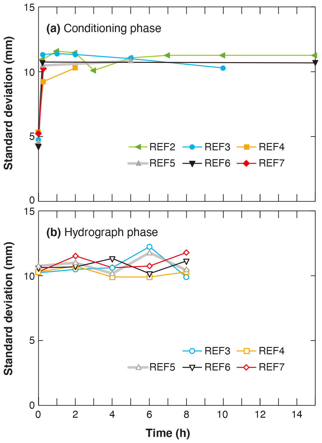
Figure 4Temporal adjustments of standard deviation of bed elevation calculated over the whole erodible bed: (a) the conditioning phase and (b) the hydrograph phase. The uncertainty of the calculation is in the range of 1.6–2.5 mm, which is close to the vertical resolution of the laser (1 mm).
Figure 5 shows the temporal variation of the characteristic grain size of bed surface material, as well as an estimation of the uncertainties associated with measurements of the surface texture. Three parameters are presented here: Ds10, Ds50, and Ds90. The adjustment of bed surface GSD follows similar trends to the adjustment of standard deviation of bed elevation; i.e., for all experiments the bed surface is fine at the beginning and experiences a fast coarsening period during the first 15 min (along with the bed degradation in Fig. 3 and the increase of bed roughness in Fig. 4). The characteristic grain sizes of bed surface remain relatively stable after the first 15 min, despite variabilities due to the measurement uncertainty. For REF2 (15), which has the longest conditioning phase, cv (coefficient of variation) values of the mean Ds10, Ds50, and Ds90 (over the five repeated measurements) are 0.15, 0.09, and 0.02, respectively, from t=15 min to the end of the conditioning flow. It is worth noting that the GSD of bed surface remains relatively constant even during the hydrograph phase, during which a flood event is introduced in the flume and evident bed degradation is observed. For each experiment, the cv values of the mean Ds10, Ds50, and Ds90 (over the five repeated measurements) are less than 0.13, 0.08, and 0.04, respectively, during the hydrograph phase.
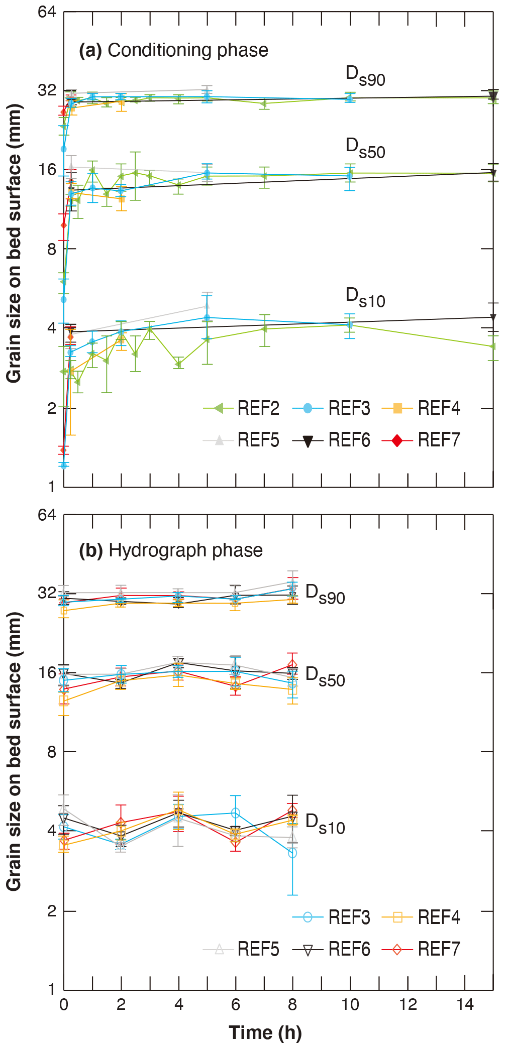
Figure 5Temporal adjustments of characteristic grain sizes of bed surface material calculated over the whole erodible bed: (a) the conditioning phase and (b) the hydrograph phase. Markers show mean values of five repeated Wolman measurements. Range bars show the mean values ± the standard deviations of the five repeated Wolman measurements.
3.2 Sediment transport
In Fig. 6 we present the instantaneous sediment transport rate Qs measured by the light table during each experiment. Sediment transport is reported every 5 min, as described in Sect. 2. Accuracy of the results is estimated by comparing the light table data with the data measured by the trap. Results show that for our experiments, the light table method has good accuracy in terms of the sediment transport rate, with an overestimation by 4 % on average (111 samples and a standard deviation of 14.5 %). A total of 70 out of 111 samples show an accuracy of ±10 %, and 93 out of 111 samples show an accuracy of ±20 %. Details of this uncertainty analysis are presented in the Supplement.
It can be seen in Fig. 6a that the temporal variation of sediment transport rate during the conditioning phase follows the same trend in all six experiments. That is, the sediment transport rate decreases significantly during the conditioning phase, with the decreasing rate being very large at the beginning and then gradually dropping. In the first 15 min, the sediment transport rates drop from more than 500 kg/h to less than 100 kg/h. Afterwards, it takes about another 2 h for the sediment transport rates to drop to close to 1 kg/h. The sediment transport rate eventually approaches a small and relatively constant value after about 8 h of conditioning flow. For REF2 (15) and REF6 (15), which have the longest conditioning phase, the sediment transport rates between t=8 h and the end of conditioning phase (t=15 h) show mean values of 0.35 kg/h (standard deviation = 0.22 kg/h) and 0.37 kg/h (standard deviation = 0.24 kg/h), respectively. Nevertheless, there are random high points in the sediment transport rate even after 8 h, despite no sediment feed from the inlet. These spikes imply that partial destruction (or reorganization) of the bed structure occurs even after a long duration of conditioning.
Previous researchers (Haynes and Pender, 2007; Masteller and Finnegan, 2017) have suggested that an exponential function can be implemented to describe such a decrease of sediment transport rate under conditioning flow. Additional analysis is implemented in the Supplement to fit REF2 (15) and REF6 (15) (which have the longest duration of conditioning phase) against a two-parameter exponential function. Results show that the exponential function can describe the general decreasing trend of sediment transport rate during the conditioning phase, except at the beginning of the experiment where the decrease of sediment transport rate is much more significant than that predicted by the exponential function. Readers can refer to the Supplement for more details.
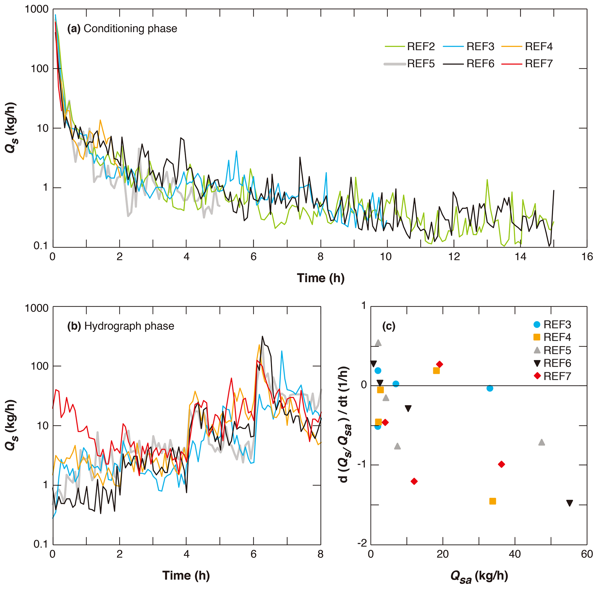
Figure 6Instantaneous sediment transport rate measured by the light table during (a) the conditioning phase and (b) the hydrograph phase. (c) Intra-step temporal change rate of Qs normalized against Qsa for each hydrograph step. Qs is the sediment transport rate, and Qsa is the averaged sediment transport rate of a given hydrograph step.
Figure 6b presents the instantaneous sediment transport rate during the hydrograph phase. Results show that variation of sediment transport rate among different experiments prevails in the first step of the hydrograph, with the highest sediment transport rate for the experiment with the shortest conditioning duration (REF7 (0.25)) and the smallest sediment transport rate for the experiment with the longest conditioning duration (REF6 (15)). Such variation among experiments, however, diminishes towards the end of step 1 and is not observed in the following three steps of the hydrograph, with the line for each experiment collapsing together in the figure. Such adjustments of sediment transport rate are consistent with the process of channel deformation shown in Fig. 3. Thus, for both sediment transport and channel deformation, results of REF7 (0.25) deviate from other experiments in step 1 (larger sediment transport rate and more degradation in REF7 (0.25)) but collapse with other experiments in the following three steps.
Results in Fig. 6b also show large variations of sediment transport rate during each step of the hydrograph. Such intra-step variations of sediment transport rate are investigated in Fig. 6c, with the x axis being the averaged sediment transport rate of each step Qsa and the y axis being d(Qs/. The value of d(Qs/ is estimated by linear regression. Here the instantaneous sediment transport rate Qs is scaled against the average sediment transport rate of the corresponding step Qsa in order to facilitate the comparison among different hydrograph steps.
Results in Fig. 6c show that a large fraction of the data (11 out of 20) exhibit a decreasing trend in time for Qs (i.e., a negative value in vertical coordinate). Basically, the larger the averaged sediment transport rate Qsa, the larger the rate of reduction in Qs. Ferrer-Boix and Hassan (2015) observed similar declines in sediment transport during their water pulse experiments. They attributed this to (1) the presence of bed structures, which could have reduced skin friction up to 20 %, and (2) streamwise changes in the patterns of bed surface sorting. Out of 20 datasets, 5 exhibit some temporally increasing trend in Qs (though this is not as evident as the decreasing trend mentioned before). They are REF5 (5), REF3 (10), REF6 (15) during the first step and REF7 (0.25), REF4 (2) during the third step. This shows that for the three experiments with a long conditioning duration, Qs is very low at the end of the conditioning phase, and the first step of the hydrograph sees a temporally increasing trend in Qs, whereas for the two experiments with a short conditioning phase, Qs is still high at the end of the conditioning, and thus the sediment transport rate keeps decreasing during the first step until an increasing trend in Qs is observed in the third step, at which point the water and sediment supply become evidently higher. The decreasing and increasing trends of Qs during steps of the hydrograph reflect the transient adjustments of the bed to the changed water and sediment supply before equilibrium is achieved.
Sediment collected in the trap or tailbox at the flume outlet allows us to plot the total amount of sediment output during each step of the hydrograph. Figure 7a shows the total sediment output during the entire hydrograph. It can be seen that the effect of conditioning duration on the total sediment output during the entire hydrograph phase is not evident: a longer duration of conditioning flow does not necessarily lead to a smaller (or larger) sediment output. The largest sediment output occurs in REF7 (0.25), which is 55 % larger than the sediment output in REF3 (10), which has the smallest output, but is about the same as (only 4 % larger than) the sediment output in REF6 (15). We further calculate the correlation coefficient between the total sediment output and the duration of conditioning flow and obtain a value of , indicating that there is almost no correlation between the two parameters.
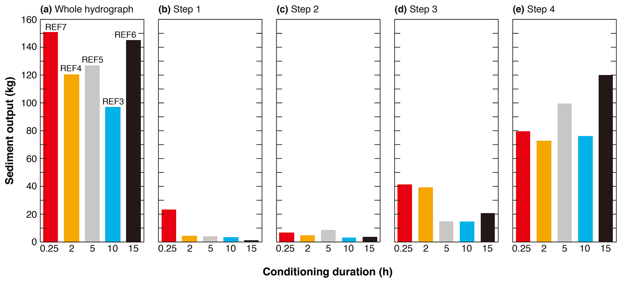
Figure 7Sediment output measured at a trap during (a) the whole hydrograph, (b) step 1 of the hydrograph, (c) step 2 of the hydrograph, (d) step 3 of the hydrograph, and (e) step 4 of the hydrograph.
However, if we study the sediment transport during each step of the hydrograph, we can find that in step 1 REF7 (0.25) has much larger sediment output than the other experiments, as shown in Fig. 7b. For Step 1, the sediment output is 1.1 in REF6 (15); 3.4–4.4 kg in REF4 (2), REF5 (5), and REF 3(10); and increases sharply to 23.4 kg in REF7 (0.25) (which is more than 20 times that in REF6 (15)). This agrees with the results for instantaneous sediment transport rate shown in Fig. 6b and shows that the duration of conditioning flow can influence the sediment transport at the beginning of the subsequent flood, with a longer conditioning phase leading to less sediment transport. When the duration of conditioning flow is over 2 h, the subsequent sediment transport rate becomes rather insensitive to further increase of conditioning duration, indicating that the reorganization of the river bed under conditioning flow is mostly finished within 2 h. The effects of stress history on subsequent sediment transport can hardly be observed during step 2 of the hydrograph (Fig. 7c). Sediment output in REF7 (0.25) reduces significantly to a similar magnitude to the other experiments because most of the loose bed material in REF7 (0.25) has been moved by the end of step 1. More specifically, the volumes of sediment output in this step range between 3.1 and 8.6 kg, with the largest output occurring in REF5 (5) and the minimum output occurring in REF3 (10). We further calculate the correlation coefficient between sediment output and conditioning duration and obtain a value of , indicating that a longer conditioning duration can no longer lead to a larger sediment output in this step. In Step 3 of the hydrograph (Fig. 7d), sediment output in REF7 (0.25) and REF4 (2) is larger than in other three experiments, which have longer conditioning phases. However, in this step the sediment output in REF7 (0.25) is no more than 3 times that of the sediment output in REF3 (10), which has the minimum sediment output. This difference of sediment output among experiments is not as significant as in step 1. In the last step of the hydrograph, with the flow discharge and sediment supply approaching their peaks, the difference in sediment output among the five experiments again becomes small, with the values ranging between 72.1 kg in REF4 (2) and 119.6 kg in REF6 (15). This demonstrates that little influence of stress history remains in this step.
Figure 8 shows the temporal variation of the grain size distribution of the bed load. Here Dl10, Dl50, and Dl90 denote grain sizes such that 10 %, 50 %, and 90 % are finer in the bed load, respectively. Accuracy of the measurements is estimated by comparing the light table data with the trap data. Results show that for our experiments, the light table method has good accuracy in terms of the median size of bed load (Dl50), with an overestimation by 3 % on average (111 samples and a standard deviation of 40.1 %). Measurements of Dl10 and Dl90 show less accuracy, with an underestimation by 20 % on average (111 samples and a standard deviation of 39.0 %) for Dl10 and an overestimation by 30 % on average (111 samples and a standard deviation of 26.5 %) for Dl90. Details concerning this uncertainty analysis are presented in the Supplement.
The value of Dl10 shows a decreasing trend during the conditioning phase (Fig. 8a), with a value of more than 2 mm at the beginning to about 0.6 mm after 15 h, in spite of the large fluctuations before 8 h. The decrease of Dl10 reflects an increase in the fraction of the finest sediment in bed load. In the first two steps of the hydrograph (Fig. 8b), the value of Dl10 is relatively stable for experiments with long conditioning phases (i.e., REF6 (15) and REF3 (10)) but shows a decreasing trend along with fluctuations for experiments with short conditioning phases (i.e., REF7 (0.25), REF4 (2), and REF5 (5)). The last two steps of the hydrograph see an evident increase in the value of Dl10 compared with the first two steps, due to the increase of flow discharge and sediment supply (Fig. 8b). We note that such an increase in the Dl10 is larger than the standard deviation of measurements, as shown above.
Figure 8c and d show the temporal variation of Dl50. Compared with that of Dl10, the temporal variation of Dl50 shows more significant fluctuations during the conditioning phase (especially after t=10 h), as well as at the beginning of the hydrograph. This can be shown by the coefficient of variation (cv) of the grain size. For the conditioning phase (after t=10 h), the cv of Dl10 shows an average value of 0.05, whereas the cv of Dl50 shows an average value of 1.44. For step 1 of the hydrograph phase, the cv of Dl10 shows an average value of 0.35, whereas the cv of Dl50 shows an average value of 0.66. For step 2 of the hydrograph phase, the cv of Dl10 shows an average value of 0.12, whereas the cv of Dl50 shows an average value of 0.54. As for the temporal variation of Dl90 (in Fig. 8e and f), the fluctuations are still significant, with the average cv being 0.61, 0.34, and 0.27 for the conditioning phase (after t=10 h), step 1 of hydrograph phase, and step 2 of hydrograph phase, respectively. Besides, there is no significant increase or decrease of Dl90 during the experiment. This indicates that the transport of the coarsest sediment is not sensitive to the variation of our experimental conditions. The more significant fluctuations in Dl50 and Dl90 might be attributed to the fact that during relatively low flow coarse sediment is more likely to be near the threshold of motion and move intermittently, e.g., as individual grains, as opposed to the more continuous movement for fine sediment. These fluctuations gradually diminish with the increase of flow and sediment supply, as the static armor on bed surface transits to mobile armor and the movement of coarse grains becomes more continuous.
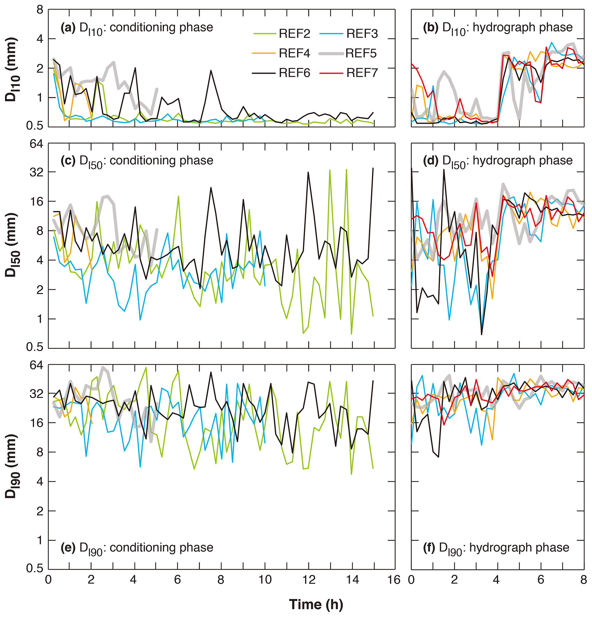
Figure 8Temporal adjustments of characteristic grain sizes of bed load: (a) Dl10 during conditioning phase, (b) Dl10 during hydrograph phase, (c)Dl50 during conditioning phase, (d) Dl50 during hydrograph phase, (e) Dl90 during conditioning phase, and (f) Dl90 during hydrograph phase.
With the fractional sediment transport rate measured by the light table, we also analyze the sediment mobility of each size range during the experiment. Results show that sediment transport rate is characterized by equal mobility (i.e., the GSD of sediment load matches the GSD of sediment on bed surface) at the beginning of the conditioning phase but moves to partial or selective mobility after a relatively long conditioning phase and during the first two steps of the hydrograph. However, with the increase of flow discharge and sediment supply, the sediment transport regime gradually returns to equal mobility during the last two steps of the hydrograph. Details of the analysis are presented in the Supplement.
4.1 Threshold of sediment motion in experiments
The threshold of sediment motion is a key parameter for the prediction of bed load transport. Previous studies on the stress history effect often start with a conditioning flow that is below the threshold of motion and then gradually increase the flow discharge so that the threshold of motion can be directly estimated in the experiment (e.g., Monteith and Pender, 2005; Masteller and Finnegan, 2017; Ockelford et al., 2019; etc.). Because our experiments implement a conditioning flow which can mobilize sediment (sediment transport at the beginning of the conditioning phase is especially large), the threshold of motion cannot be observed directly in the experiment. Here we follow the method applied in Hassan et al. (2020) and estimate the threshold of sediment motion with the Wong and Parker (2006) sediment transport relation, which is a revision of the Meyer-Peter and Müller (1948) relation.
We use the Wong and Parker (2006) relation, which maintains the exponent 1.5 of Meyer-Peter and Muller (1948):
where is the dimensionless bed load transport rate (Einstein number) defined by Eq. (2), is the Shields number for surface median grain size Ds50 defined by Eq. (3), τb is the flow shear stress calculated using the depth–slope product (Eq. 4), is the critical Shields number for the threshold of sediment motion, qs is the volumetric sediment transport rate per unit width, h is water depth, Sw is water surface slope, R=1.65 is the submerged specific gravity of sediment, g=9.81 m/s2 is the gravitational acceleration, and ρ=1000 kg/m3 is the water density. Wong and Parker (2006) proposed a value of 0.0495 for in Eq. (1). Here we obtain and from the measured data of the experiments and back-calculate the value of using Eq. (1). It is worth mentioning that in Hassan et al. (2020) three different methods, including the method as described above, are applied to estimate the threshold of sediment motion. Estimations with the three different methods show a very similar temporal trend and variability.
Figure 9a shows the values of vs. for each experiment, along with the Wong and Parker (2006) type relation (Eq. 1) with various values for (from 0.04 to 0.09). It can be seen from the figure that the measured sediment transport rate is relatively low, with most points below the dimensionless value of 0.001. This indicates that the Shields number in our experiment is slightly larger than the critical Shields number, a state that is typical for gravel-bed rivers (Parker, 1978). The four points with dimensionless transport rate above 0.001 are all at the beginning of the conditioning flow (t=15 min). The values of basically show an increasing trend with the increase of , with the correlation coefficient between and log() (consistent with the semi-log scale of Fig. 9a) being 0.58. Besides, the values of critical Shields number shown in Fig. 9a cover a rather wide range (from less than 0.06 to larger than 0.09).
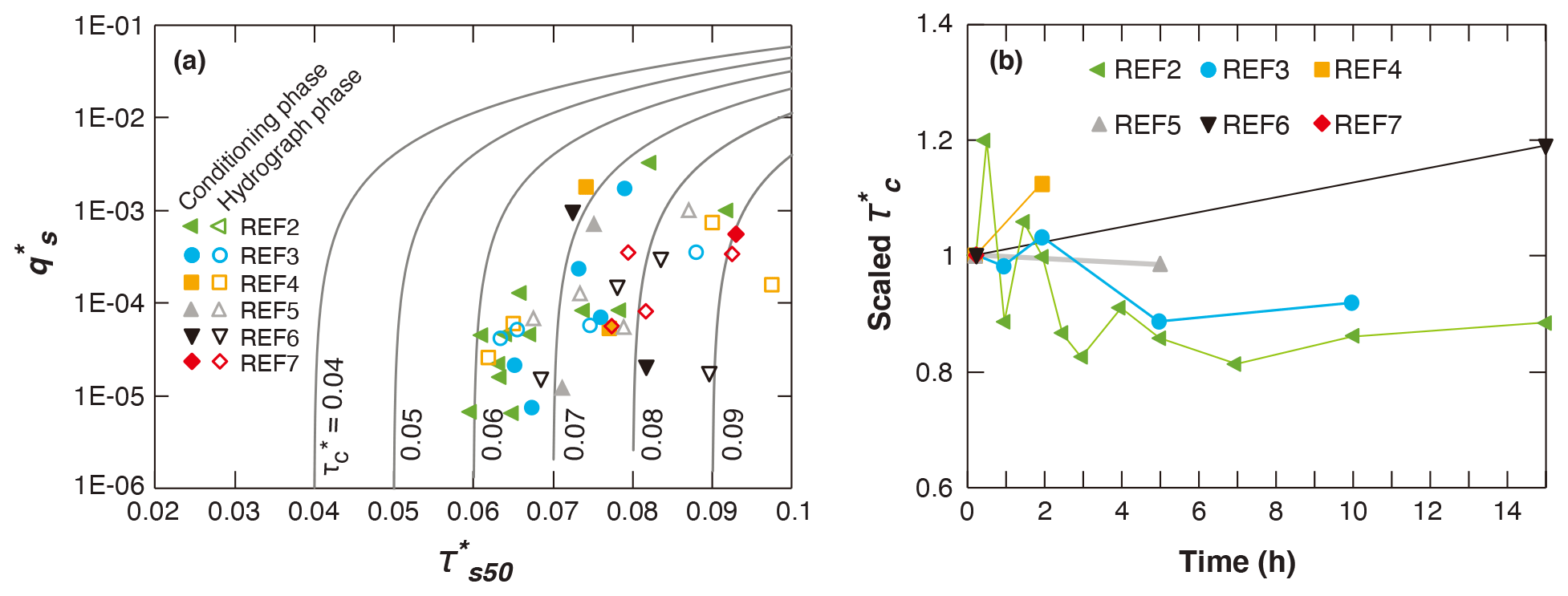
Figure 9(a) Dimensionless sediment transport rate vs. Shields number using surface median grain size for measured transport rates (points). Also shown are lines for the Wong and Parker (2006) type equation (Eq. 1) using different values for . (b) Temporal adjustment of scaled ( over at 15 min) during the conditioning phase. Here is back-calculated using Eq. (1) (Wong and Parker, 2006, relation).
Table 2 shows the values of back-calculated at the beginning (t=15 min) and the end of the conditioning phase in each experiment. The back-calculated values of vary in the range 0.065–0.090 for the conditioning phase, which is well above the value of 0.0495 recommended by Wong and Parker (2006). Lamb et al. (2008) demonstrated that critical shear stress can become larger for large bed slope, and they proposed a relation which considers the effect of bed slope,
where Sb is bed slope. For comparison, Table 2 also shows the values of calculated by Eq. (5). Results shows that for the conditioning phase of our experiments, calculated by Eq. (5) is above 0.06, which is much higher than the recommended value of Wong and Parker (2006). Besides, the values predicted by the Lamb et al. (2008) relation show little variability among different experiments, compared with the values back-calculated with Eq. (1) based on experimental data. More specifically, the cv values are 0.032 at t=15 min and 0.031 at the end of the conditioning phase for predicted by Lamb et al. (2008) relation but become 0.10 at t=15 min and 0.12 at the end of the conditioning phase for back-calculated with Eq. (1) using measured data. Such discrepancies could be ascribed to the fact the relation of Lamb et al. (2008) considers only the influence of bed slope, without considering the effects of other mechanisms like organization of surface texture, infiltration of fine particles, etc. These potential effects are discussed in more detail in Sect. 4.2.
Here we also estimate the uncertainties associated with the calculation of . For back-calculated with Eq. (1), the global uncertainty is estimated by combining the uncertainties of each parameter involved in the calculation, i.e., water depth h, water surface slope Sw, sediment transport rate qs, and surface median grain size Ds50. The applied ranges of h and Sw are the measured values plus or minus the errors associated with the gauge point. The applied ranges of qs and Ds50 are the measured values plus or minus the standard deviations as reported in Sect. 3. Results of the uncertainties are presented in the brackets in Table 2. For the values calculated with Eq. (5), the uncertainties are only from the bed slope Sw (which is related with the resolution of point gauge) and are lower than ±1 % according to our estimates. Therefore, the uncertainty of calculated with the Eq. (5) is not presented in the table. It can be seen from Table 2 that the values of calculated with the Eq. (5) are mostly within the uncertainty range of back-calculated with Eq. (1), with the values closer to the lower bound of the uncertainty range.
Table 2Values of at the beginning (t=15 min) and the end of conditioning phase in each experiment. Here is back-calculated with Eq. (1). Also shown here are values of estimated with the equation of Lamb et al. (2008) for comparison. Values in the brackets denote the range of uncertainty associated with the values back-calculated with Eq. (1).

In Fig. 9b, we plot the scaled during the conditioning phase of our experiments. For each experiment, the scaled is calculated as the ratio between and the corresponding at t=15 min. implemented here is back-calculated with Eq. (1). The scaled collapses on a value of unity at t=15 min (i.e., the first point of each experiment). It can be seen from Fig. 9 that different trends are exhibited for the adjustment of from t=15 min to the end of conditioning phase, with REF2 (15) and REF3 (10) exhibiting a decreasing trend, REF5 (5) exhibiting very slight changes, and REF4 (2) and REF6 (15) exhibiting an increasing trend. The decrease of in REF2 (15) and REF3 (10) is accompanied by a reduction of Shields number , mainly due to the increase of surface median grain size Ds50. Moreover, the variation of back-calculated is mostly within a range of ±20 %, in agreement with our observation that variation of bed topography and bed surface texture become insignificant after 15 min. It should be noted that cannot be back-calculated using Eq. (1) within the first 15 min of the conditioning phase, since the information for flow depth, water surface slope, and bed surface GSD is not available. Nevertheless, we expect the adjustment of could be evident within the first 15 min, since the adjustments of both bed topography and bed surface are significant during this period (as shown in Sect. 3.1).
4.2 Implications and limitations
Previous research has shown that antecedent conditioning flow can lead to an increased critical shear stress and reduced sediment transport rate during subsequent flood event (Hassan and Church, 2000; Haynes and Pender, 2007; Ockelford and Haynes, 2013; Masteller and Finnegan, 2017). Our flume experiments also show a reduction in sediment transport rate, especially at the beginning of the hydrograph, in response to the implementation of antecedent conditioning flow (as shown in Figs. 6b and 7). However, our results are different from previous research in that the influence of antecedent conditioning flow is found to last for a relatively short time at the beginning of the following hydrograph and then gradually diminish with the increase of flow intensity and sediment supply (Figs. 6 and 7). Such results indicate that increasing flow intensity and sediment supply during a flood event can lead to the loss of memory of stress history. A similar phenomenon was observed by Mao (2018) in his experiment, where sediment transport during a high-magnitude flood event was not affected much by the occurrence of lower-magnitude flood event before. Besides, the subsequent hydrograph leads to evident bed degradation (Fig. 3) and increase of sediment transport rate (Figs. 6 and 7) but does not lead to evident change of surface texture or break of the armor layer (Fig. 5). This is in agreement with the observation of Ferrer-Boix and Hassan (2015) during experiments of successive water pulses.
Our results have practical implications for mountain gravel-bed rivers. The importance of conditioning flow has long been discussed in the literature, and researchers have suggested that the stress history effect be considered in the modeling and analysis of gravel-bed rivers. For example, previous research states that existing sediment transport theory for gravel-bed rivers (e.g., Meyer-Peter and Müller, 1948; Wilcock and Crowe, 2003; Wong and Parker, 2006; etc.) might lead to unrealistic predictions if the stress history effect is not taken into account (Masteller and Finnegan, 2017; Mao, 2018; Ockelford et al., 2019). Our results indicate that the stress history effect is important and needs to be considered for low flow and the beginning of the flood event but becomes insignificant as the flow gradually approaches high flow discharge.
To explain the effect of stress history, Ockelford and Haynes (2013) have summarized the following possible mechanisms. (1) Vertical settling during the conditioning flow consolidates the bed into a tighter packing arrangement that is more resistant to entrainment. (2) Local reorientation and rearrangement of surface particles provide a greater degree of imbrication, less resistance to fluid flow, and direct sheltering on the bed surface. (3) The infiltration of fine particles into low-relief pore spaces can further increase the bed compaction. In the experiment of Masteller and Finnegan (2017), it was found that the most drastic changes during conditioning flow are manifested in the extreme tail of the elevation distribution (i.e., the reorientation of the highest protruding grains into nearby available pockets) and therefore go undetected in most bulk measurements (e.g., the mean bed elevation, standard deviation of bed topography, or the bed surface GSD). They demonstrated that such reorganization of the highest protruding grains can indeed lead to noticeable differences in the threshold of sediment transport (Masteller and Finnegan, 2017). This might explain the observation in our experiment that after the first 15 min of the conditioning phase, adjustments of the bed topography and the bed surface GSD become insignificant, but the sediment transport rate and its GSD keep adjusting consistently.
In our experiments and previous experiments that study the effect conditioning flow (e.g., Monteith and Pender, 2005; Masteller and Finnegan, 2017; Ockelford et al., 2019), no sediment supply is implemented during the conditioning flow, and the flow can reorganize the bed surface to a state that is more resistant to sediment entrainment. Therefore, it is straightforward to expect the conclusions based on our flume experiments to apply for natural rivers where sediment supply is relatively low during low flow conditions. However, some gravel-bed rivers have quite active hillslopes, and sediment input from hillslopes to river channel can occur regularly (Turowski et al., 2011; Reid et al., 2019). Since the sediment material from hillslopes is typically loose and easy to transport, under such circumstances a long inter-event duration (i.e., low-flow duration) might lead to an enhanced sediment transport rate in the subsequent flood (Turowski et al., 2011).
It should also be noted that in previous experiment on the stress history effect, conditioning flow is often set below the threshold of sediment motion. One exception is the experiment of Haynes and Pender (2007) in which the conditioning flow was above the threshold of motion for D50. By implementing conditioning flow with various durations and magnitudes, they demonstrated that a longer duration of conditioning flow will increase the bed stability, whereas a higher magnitude of conditioning flow will reduce the bed stability. However, since the subsequent flow they implement to test the bed stability was constant through time, their results did not show how a subsequent flow event with increasing intensity would affect the stress history. Here we implement a conditioning flow that can mobilize sediment, especially at the beginning of the conditioning phase, during which evident sediment transport occurs. Moreover, by implementing a subsequent (rising limb of) hydrograph, we find that the stress history can persist during the beginning of the hydrograph but is eventually erased out as the flow intensity increases. In our experiments, we varied the duration of conditioning flow by fixing the conditioning flow magnitude. In this sense, how the stress history formed under various magnitudes of conditioning flow (both above and below the threshold) would be affected by a subsequent hydrograph still merits future research.
Recently, Church et al. (2020) drew attention to the reproducibility of results in geomorphology. They distinguished three levels of “reproducibility”, including “repetition”, “replication”, and “reproduction”. In this paper, the repetition of experimental results is tested by repeating the conditioning phase with the longest duration (REF6 (15) and REF2 (15)). The two experiments show similar results during the conditioning phase in terms of standard deviation of bed elevation, GSD of bed surface, sediment transport rate, and GSD of sediment load. However, the reproduction of the experimental results, which requires independent tests undertaken using different materials and/or different conditions of measurement and is more significant, according to Church et al. (2020), for advancing of the science, has not been tested in this paper. In this regard, more effort is needed in future studies to test the reproducibility of the conclusions given in this paper.
In this paper, the effect of antecedent conditioning flow (i.e., the effect of stress history) on the morphodynamics of gravel-bed rivers during subsequent floods is studied via flume experimentation. The experiment described here is designed based on the conditions of East Creek, Canada. The experiment consisted of two phases: a conditioning phase with constant water discharge and no sediment supply, followed by a hydrograph phase with hydrograph and sedimentograph. Five runs (REF 3–7) were conducted with identical experimental conditions but different conditioning phase durations. Another run (REF 2) that consisted of only the conditioning phase was conducted in order to test the reproducibility of experimental results during the conditioning flow. Experimental results show the following.
-
Adjustments of channel morphology (including channel bed longitudinal profile, standard deviation of bed elevation, and characteristic grain sizes of bed surface material) are evident during the first 15 min of the conditioning phase but become insignificant during the remainder of the conditioning phase.
-
The implementation of conditioning flow can indeed lead to a reduction in sediment transport during the subsequent hydrograph, which agrees with previous research.
-
However, the effect of stress history on sediment transport rate is limited to a relatively short time at the beginning of the hydrograph, and gradually diminishes with the increase of flow discharge and sediment supply, indicating a loss of memory of stress history under high flow discharge. In addition, the effect of stress history on the GSD of both bed surface and bed load is not evident.
-
The threshold of sediment motion is estimated with the form of the Wong and Parker (2006) relation. The estimated critical Shields number varies in the range 0.066–0.086 during the conditioning phase (excluding the first 15 min) and is higher than the value recommended by Wong and Parker (2006).
Our study has implications in regard to a wide range of issues for mountain gravel-bed rivers, including sediment budget analysis, river morphodynamic modeling, water and sediment regulation, flood management, and ecological restoration schemes.
| Dl50 | grain size such that 50 % of the sediment load is finer (similarly, Dl10 is such that 10 % of the sediment load is finer, and Dl90 is such that 90 % of the sediment load is finer) |
| Ds50 | grain size such that 50 % of the bed surface is finer (similarly, Ds10 is such that 10 % of the bed surface is finer, and Ds90 is such that 90 % of the bed surface is finer) |
| Fr | Froude number |
| g | gravitational acceleration |
| h | water depth |
| Qs | sediment transport rate |
| qs | volumetric sediment transport rate per unit width |
| dimensionless bed load transport rate (Einstein number) | |
| R | submerged specific gravity of sediment |
| Sb | bed slope |
| Sw | water surface slope |
| ρ | water density |
| Δzb | mean difference of bed elevation |
| τb | bed shear stress |
| critical Shields number for the threshold of sediment motion | |
| dimensionless shear stress (Shields number) of the Ds50 |
Data used for the analysis can be found at the following DOI: https://doi.org/10.6084/m9.figshare.12758414 (An, 2020).
The supplement related to this article is available online at: https://doi.org/10.5194/esurf-9-333-2021-supplement.
MAH and XF designed the research. CFB performed the experiments. CA processed and analyzed the experimental data. CA prepared the manuscript with contributions from all coauthors.
The authors declare that they have no conflict of interest.
Gary Parker provided constructive comments and helped edit this paper. Maria A. Elgueta-Astaburuaga helped conduct the experiments. Rick Ketler provided support with the equipment and data collection. Eric Leinberger provided support in designing the figures. We thank Jens Turowski and another anonymous reviewer for their constructive comments, which helped us greatly improve the paper.
This research has been supported by the National Natural Science Foundation of China (grant nos. 52009063, U20A20319, 91747207) and the China Postdoctoral Science Foundation (grant no. 2018M641368).
This paper was edited by Francois Metivier and reviewed by Jens Turowski and one anonymous referee.
An, C.: Experimental data on sediment transport and channel adjustment in a gravel-bed river: stress history effect, https://doi.org/10.6084/m9.figshare.12758414, 2020.
Carling, P. A., Kelsey, A., and Glaister, M. S.: Effect of bed roughness, particle shape and orientation on initial motion criteria, in: Dynamics of Gravelbed Rivers, edited by: Billi, P., Hey, R. D., Thorne, C. R., and Tacconi, P., John Wiley & Sons, Chichester, UK, 2339, 1992.
Chartrand, S. M., Jellinek, A. M., Hassan, M. A., and Ferrer-Boix, C.: Morphodynamics of a width-variable gravel bed stream: New insights on pool-riffle formation from physical experiments, J. Geophys. Res.-Earth, 123, 2735–2766, https://doi.org/10.1029/2017JF004533, 2018.
Chen, X., Hassan, M. A., An, C., and Fu, X.: Rough correlations: Meta-analysis of roughness measures in gravel bed rivers, Water Resour. Res., 56, e2020WR027079, https://doi.org/10.1029/2020WR027079, 2020.
Chin, A., Anderson, S., Collison, A., Ellis-Sugai, B. J., Haltiner, J. P., Hogervorst, J. B., Kondolf, G. M., O'Hirok, L. S., Purcell, A. H., Riley, A. L., and Wohl E.: Linking theory and practice for restoration of steppool streams, Environ. Manage., 43, 645–661, https://doi.org/10.1007/s00267-008-9171-x, 2009.
Church, M., Dudill, A., Venditti, J. G., and Frey, P.: Are Results in Geomorphology Reproducible?, J. Geophys. Res.-Earth, 125, e2020JF005553, https://doi.org/10.1029/2020JF005553, 2020.
Curran, J. C. and Wilcock, P. R.: Effect of sand supply on transport rates in a gravel-bed channel, J. Hydraul. Eng., 131, 961–967, https://doi.org/10.1061/(ASCE)0733-9429(2005)131:11(961), 2005.
Elgueta-Astaburuaga, M. A. and Hassan, M. A.: Experiment on temporal variation of bed load transport in response to changes in sediment supply in streams, Water Resour. Res., 53, 763–778, https://doi.org/10.1002/2016WR019460, 2017.
Ferrer-Boix, C. and Hassan, M. A.: Influence of the sediment supply texture on morphological adjustments in gravel-bed rivers, Water Resour. Res., 50, 8868–8890, https://doi.org/10.1002/2013WR015117, 2014.
Ferrer-Boix, C. and Hassan, M. A.: Channel adjustments to a succession of water pulses in gravel bed rivers, Water Resour. Res., 51, 8773–8790, https://doi.org/10.1002/2015WR017664, 2015.
Gomez, B. and Church, M.: An assessment of bed load sediment transport formulae for gravel rivers, Water Resour. Res., 25, 1161–1186, https://doi.org/10.1029/WR025i006p01161, 1989.
Hassan, M. A. and Church, M.: Experiments on surface structure and partial sediment transport on a gravel bed, Water Resour. Res., 36, 1885–1895, 2000.
Hassan, M. A., Saletti, M., Johnson, J. P. L., Ferrer-Boix, C., Venditti, J. G., and Church, M.: Experimental insights into the threshold of motion in alluvial channels: sediment supply and streambed state, J. Geophys. Res.-Earth, 125, e2020JF005736, https://doi.org/10.1029/2020JF005736, 2020.
Haynes, H. and Pender, G.: Stress history effects on graded bed stability, J. Hydraul. Eng., 33, 343–349, 2007.
Howard, A.: A detachment-limited model of drainage basin evolution, Water Resour. Res., 30, 2261–2285, 1994.
Johnson, J. P. L.: Gravel threshold of motion: a state function of sediment transport disequilibrium?, Earth Surf. Dynam., 4, 685–703, https://doi.org/10.5194/esurf-4-685-2016, 2016.
Klingeman, P. C. and Emmett, W. W.: Gravel bedload transport processes, in: Gravel-Bed Rivers, edited by: Hey, R. D., Bathurst, J. C., and Thorne, C., John Wiley & Sons, Chichester, UK, 141–180, 1982.
Lamb, M. P., Dietrich, W. E., and Venditti, J. G.: Is the critical Shields stress for incipient sediment motion dependent on channel-bed slope?, J. Geophys. Res.-Earth, 113, F02008, https://doi.org/10.1029/2007JF000831, 2008.
Lenzi, M. A.: Step–pool evolution in the Rio Cordon, northeastern Italy, Earth Surf. Proc. Land., 26, 991–1008, https://doi.org/10.1002/esp.239, 2001.
Mao, L.: The effects of flood history on sediment transport in gravel bed rivers, Geomorphology, 322, 192–205, https://doi.org/10.1016/j.geomorph.2018.08.046, 2018.
Marston, R. A.: Land, life, and environmental change in mountains, Ann. Assoc. Am. Geogr., 98, 507–520, https://doi.org/10.1080/00045600802118491, 2008.
Masteller, C. C. and Finnegan, N. J.: Interplay between grain protrusion and sediment entrainment in an experimental flume, J. Geophys. Res.-Earth, 122, 274–289, https://doi.org/10.1002/2017GL076747, 2017.
Masteller, C. C., Finnegan, N. J., Turowski, J. M., Yager, E. M., and Rickermann, D.: History dependent threshold for motion revealed by continuous bedload transport measurements in a steep mountain stream, Geophys. Res. Lett., 46, 2583–2591, 2019.
Monteith, H. and Pender, G.: Flume investigation into the influence of shear stress history, Water Resour. Res., 41, W12401, https://doi.org/10.1029/2005WR004297, 2005.
Montgomery, D. R. and Buffington, J. M.: Channel-reach morphology in mountain drainage basins, Geol. Soc. Am. Bull., 109, 596–611, https://doi.org/10.1130/0016-7606(1997)109<0596:CRMIMD>2.3.CO;2, 1997.
Montgomery, D. R., Buffington, J. M., Peterson, N. P., Schuett-Hames, D., and Quinn, T. P.: Stream-bed scour, egg burial depths, and the influence of salmonid spawning on bed surface mobility and embryo survival, Can. J. Fish. Aquat. Sci., 53, 1061–1070, 1996.
Meyer-Peter, E. and Müller, R.: Formulas for bed-load transport, in: Proceedings of the 2nd Congress of International Association for Hydraulic Structures Research, Stockholm, Sweden, 7–9 June 1948, 39–64, 1948.
Ockelford, A. and Haynes, H.: The impact of stress history on bed structure, Earth Surf. Proc. Land., 38, 717–727, https://doi.org/10.1002/esp.3348, 2013.
Ockelford, A., Woodcock, S., and Haynes, H.: The impart of inter-flood duration on non-cohesive sediment bed stability, Earth Surf. Proc. Land., 44, 2861–2871, https://doi.org/10.1002/esp.4713, 2019.
Paola, C., Heller, P. L., and Angevine, C. L.: The large-scale dynamics of grain-size variation in alluvial basins, I: Theory, Basin Research, 4, 73–90, 1992.
Parker, G.: Surface-based bedload transport relation for gravel rivers, J. Hydraul. Res., 28, 417–436, https://doi.org/10.1080/00221689009499058, 1990.
Papangelakis, E. and Hassan, M. A.: The role of channel morphology on the mobility and dispersion of bed sediment in a small gravel-bed stream, Earth Surf. Proc. Land., 41, 2191–2206, 2016.
Paphitis, D. and Collins, M. B.: Sand grain threshold, in relation to bed stress history: an experimental study, Sedimentology, 52, 827–838, 2005.
Parker, G.: Self-formed straight rivers with equilibrium banks and mobile bed. Part 2. The gravel river, J. Fluid Mech., 89, 127–146, 1978.
Parker, G.: 1D sediment transport morphodynamics with applications to rivers and turbidity currents, available at: http://hydrolab.illinois.edu/people/parkerg//morphodynamics_e-book.htm (last access: 17 April 2021), 2004.
Powell, D. M., Reid, I., and Laronne, J. B.: Hydraulic interpretation of crossstream variations in bed-load transport, J. Hydraul. Eng., 125, 1243–1252, 1999.
Reid, D. A., Hassan, M. A., Bird, S., and Hogan D.: Spatial and temporal patterns of sediment storage over 45 years in Carnation Creek, BC, a previously glaciated mountain catchment, Earth Surf. Proc. Land., 44, 1584–1601, https://doi.org/10.1002/esp.4595, 2019.
Reid, I. and Frostick, L. E.: Particle interaction and its effects on the thresholds of initial and final bedload motion in coarse alluvial channels, in: Sedimentology of Gravels and Conglomerates-Memoir 10, edited by: Koster, E. H. and Steel, R. J., Canadian Society of Petroleum Geologists, Calgary, Canada, 61–68, 1984.
Reid, I., Frostick, L. E., and Layman, J. T.: The incidence and nature of bedload transport during flood flows in coarse-grained alluvial channels, Earth Surf. Proc. Land., 10, 33–44, 1985.
Rickenmann, D.: Comparison of bed load transport in torrents and gravel bed streams, Water Resour. Res., 37, 3295–3305, https://doi.org/10.1029/2001WR000319, 2001.
Schneider, J. M., Rickenmann, D., Turowski, J. M., Bunte, K., and Kirchner, J. W.: Applicability of bed load transport models for mixed-size sediments in steep streams considering macro-roughness, Water Resour. Res., 51, 5260–5283, https://doi.org/10.1002/2014wr016417, 2015.
Sklar, L. and Dietrich W. E.: A mechanistic model for river incision into bedrock by saltating bed load, Water Resour. Res., 40, W06301, https://doi.org/10.1029/2003WR002496, 2004.
Turowski, J. M., Yager, E. M., Badoux, A., Rickenmann, D., and Molnar, P.: The impact of exceptional events on erosion, bedload transport and channel stability in a step-pool channel, Earth Surf. Proc. Land., 34, 1661–1673, https://doi.org/10.1002/esp.1855, 2009.
Turowski, J. M., Badoux, A., and Rickenmann, D.: Start and end of bedload transport in gravel-bed streams, Geophys. Res. Lett., 38, L04401, https://doi.org/10.1029/2010GL046558, 2011.
Venditti, J. G., Dietrich, W. E., Nelson, P. A., Wydzga, M. A., Fadde, J., and Sklar, L.: Mobilization of coarse surface layers in gravel-bedded rivers by finer gravel bed load, Water Resour. Res., 46, W07506, https://doi.org/10.1029/2009WR008329, 2010.
Whiting, P. J. and Dietrich, W. E.: Boundary shear stress and roughness over mobile alluvial beds, J. Hydraul. Eng., 116, 1495–1511, 1990.
Wilcock, P. R. and Crowe, J. C.: Surface-based transport model for mixed-size sediment, J. Hydraul. Eng.-ASCE, 129, 120–128, https://doi.org/10.1061/(asce)0733-9429(2003)129:2(120), 2003.
Wilcock, P. R., Kenworthy, S. T., and Crowe, J. C.: Experimental study of the transport of mixed sand and gravel, Water Resour. Res., 37, 3349–3358, 2001.
Wong, M. and Parker, G.: Reanalysis and correction of bed-load relation of Meyer-Peter and Müller using their own database, J. Hydraul. Eng.-ASCE, 132, 1159–1168, https://doi.org/10.1061/(ASCE)0733-9429(2006)132:11(1159), 2006.
Yager, E. M., Turowski, J. M., Rickenmann, D., and McArdell, B. W.: Sediment supply, grain protrusion, and bedload transport in mountain streams, Geophys. Res. Lett., 39, L10402, https://doi.org/10.1029/2012GL051654, 2012.
Zimmermann, A., Church, M., and Hassan, M. A.: Video-based gravel transport
measurements with a flume mounted light table, Earth Surf. Proc. Land., 33, 2285–2296,
doi10.1002/esp.1675,
2008.