the Creative Commons Attribution 4.0 License.
the Creative Commons Attribution 4.0 License.
 | 24 Jun 2021
Precise water level measurements using low-cost GNSS antenna arrays
David J. Purnell
Natalya Gomez
William Minarik
David Porter
Gregory Langston
We have developed a ground-based Global Navigation Satellite System Reflectometry (GNSS-R) technique for monitoring water levels with a comparable precision to standard tide gauges (e.g. pressure transducers) but at a fraction of the cost and using commercial products that are straightforward to assemble. As opposed to using geodetic-standard antennas that have been used in previous GNSS-R literature, we use multiple co-located low-cost antennas to retrieve water levels via inverse modelling of signal-to-noise ratio data. The low-cost antennas are advantageous over geodetic-standard antennas not only because they are much less expensive (even when using multiple antennas in the same location) but also because they can be used for GNSS-R analysis over a greater range of satellite elevation angles. We validate our technique using arrays of four antennas at three test sites with variable tidal forcing and co-located operational tide gauges. The root mean square error between the GNSS-R and tide gauge measurements ranges from 0.69–1.16 cm when using all four antennas at each site. We find that using four antennas instead of a single antenna improves the precision by 30 %–50 % and preliminary analysis suggests that four appears to be the optimum number of co-located antennas. In order to obtain precise measurements, we find that it is important for the antennas to track GPS, GLONASS and Galileo satellites over a wide range of azimuth angles (at least 140∘) and elevation angles (at least 30∘). We also provide software for analysing low-cost GNSS data and obtaining GNSS-R water level measurements.
- Article
(4684 KB) - Full-text XML
-
Supplement
(610 KB) - BibTeX
- EndNote


Precise water level measurements are needed for monitoring the global oceans, lakes and rivers, all of which are vulnerable to anthropogenic climate change (Goudie, 2006; Adrian et al., 2009; Slangen et al., 2016). Sea level at any location is influenced by spatiotemporally variable processes such as tides, storm surges and glacial isostatic adjustment (Tamisiea et al., 2014; Kopp et al., 2015). Networks of coastal water level sensors are therefore necessary to validate models of these processes (Meyssignac et al., 2017; Seifi et al., 2019; Dullaart et al., 2020) and satellite altimetry measurements (Gómez-Enri et al., 2018; Peng and Deng, 2020). The need for precise water level measurements was recently highlighted by Taherkhani et al. (2020), who showed that even a modest sea level rise of 1 cm in some regions could double the odds of a 50-year extreme water level event (i.e. a flooding event). The risk posed by extreme water level events is especially concerning given that current projections of globally averaged sea level rise by 2100 due to mass changes from the Antarctic ice sheet alone vary from 0 to 1.7 m (Pattyn and Morlighem, 2020), whilst projections of mass loss from Greenland's largest outlet glaciers for the same period may be underestimated (Khan et al., 2020). Continuous records of sea level changes in the polar regions that could be used to constrain the response of ice sheets to ongoing climate change remain critically sparse (Baumann et al., 2020).
A range of different instruments are commonly used for monitoring water levels with variable cost and accuracy (GLOSS, 2012; Míguez et al., 2005; Pytharouli et al., 2018). With a budget of approximately USD 1000–10 000, it is possible to buy an acoustic gauge or a pressure gauge to monitor water levels with sub-centimetre accuracy – the level of accuracy required for the Global Sea Level Observing System (GLOSS) network (GLOSS, 2012). However, pressure gauges may suffer from drift over multi-year timescales (Míguez et al., 2005; Pytharouli et al., 2018), and acoustic gauges are difficult to install in remote regions because they require a structure to hang over the water surface. Radar and bubbler gauges are also commonly used to monitor water levels (see Woodworth and Smith, 2003, for a comparison), but these instruments are more expensive than pressure transducers or acoustic gauges. Global Navigation Satellite System Reflectometry (GNSS-R) is an alternative technique to monitor water levels using geodetic-standard antennas that were designed to monitor land deformation. These instruments can be purchased within the same budget as previously mentioned for acoustic or pressure sensors and do not suffer from the same issues. There are already many geodetic-standard antennas installed in remote regions to monitor earth deformation and a recent study demonstrated that coastal antennas in Greenland and Antarctica could also be used to monitor sea level (Tabibi et al., 2020). However, in previous studies the precision of GNSS-R water level measurements was found to be worse than 1 cm and the datum of measurements is generally undefined (Larson et al., 2013; Strandberg et al., 2016; Tabibi et al., 2020; Purnell et al., 2020).
Recently, as part of a broader trend in environmental sensing, there has been interest in the use of mobile devices and low-cost instrumentation for monitoring water levels. For example, Sermet et al. (2020) used images captured on smartphones to make river stage measurements, and Strandberg and Haas (2019) applied GNSS-R techniques to make sea level measurements using the built-in GNSS antenna on a tablet computer. The latter study found comparable precision to GNSS-R measurements from a co-located geodetic-standard antenna. Fagundes et al. (2021) applied GNSS-R techniques to monitor a lake in Brazil using instruments that cost approximately USD 200 and found a root mean square error (RMSE) of 2.9 cm when compared to approximately 1 year of measurements from a co-located radar gauge. Similarly, Williams et al. (2020) mounted a low-cost GPS receiver and antenna near a tide gauge in Ireland and found an RMSE of 5.7 cm when comparing measurements taken over a 2-year period. The larger RMSE found by Williams et al. (2020) compared to Fagundes et al. (2021) can be at least partly accounted for by the larger daily water level variations at the coastal site in Ireland due to ocean tides.
Low-cost GNSS antennas such as those used by Strandberg and Haas (2019), Fagundes et al. (2021) and Williams et al. (2020) have been shown to be better suited for GNSS-R than geodetic-standard antennas because geodetic-standard antennas are designed to reduce multipath interference (the signal that is analysed for GNSS-R measurements). Geodetic-standard antennas can only be used to make water level measurements at low elevation angles (often less than 20∘), whereas low-cost antennas are designed for mobile devices; hence they are approximately isotropic in their gain pattern and can be used at larger elevation angles. The extra data at larger elevation angles are useful because the bias caused by tropospheric delay (or atmospheric refraction) is reduced at larger elevation angles (Santamaría-Gómez and Watson, 2017; Williams and Nievinski, 2017; Nikolaidou et al., 2020). According to Nikolaidou et al. (2020), the tropospheric altimetry bias varies from 5 cm to 3 mm for an antenna that is 10 m above a reflecting surface when using elevation angles larger than 20∘. Using data collected at elevation angles larger than 20∘ could help to eliminate the need for complicated tropospheric delay corrections that rely on global models with poor spatial resolution (Williams and Nievinski, 2017) or additional instrumentation to make in situ measurements (Santamaría-Gómez and Watson, 2017).
Purnell et al. (2020) recently showed that random noise in the signal-to-noise ratio (SNR) is one of the dominant sources of uncertainty in GNSS-R water level measurements, particularly at high elevation angles. Their results suggest that multiple co-located antennas could be used to cancel out the effect of random noise in the SNR data and improve the precision of water level measurements. It would be prohibitively expensive to co-locate several geodetic-standard antennas for the purpose of cancelling out the effect of random noise, but multi-frequency, weatherproof GNSS antennas are commercially available online for USD 10–30, meaning that multiple low-cost antennas are still a fraction of the cost of a single geodetic-standard antenna.
The purpose of this study is to test the hypothesis that multiple co-located antennas can be used to improve the precision of GNSS-R water level measurements and to demonstrate the effectiveness of low-cost antennas. We test this hypothesis by retrieving water level measurements from arrays of four stacked low-cost antennas at three different locations with variable tidal forcing and compare the measurements with nearby operational tide gauges. Section 2 contains a summary of the technique that was developed by Strandberg et al. (2016) to retrieve sea level measurements using inverse modelling of SNR data and a description of how we adapted it for using multiple co-located antennas. In Sect. 3 we provide a description of the arrays of four stacked low-cost antennas that we used to retrieve water level measurements, and in Sect. 4 we describe the three test sites. Finally in Sect. 5 we present our results from the test sites and in Sect. 6 we discuss a range of parameters related to the GNSS-R analysis in order to guide future installations.
An antenna with a view of a water surface simultaneously receives GNSS signals that travel directly from a satellite and signals that reflect off the water surface prior to reaching the antenna. As a satellite moves in orbit, the difference in path length between the direct and reflected signals changes and the signals arrive at the antenna periodically in and out of phase, thereby causing an oscillation in the SNR. For each period that a GNSS satellite is aligned with the water surface such that the antenna receives reflected signals, Larson et al. (2013) showed that the SNR can be represented as a function of the elevation angle of the satellite and the height of the antenna above the reflecting surface;
where δSNR is the detrended SNR, A depends on the power of the reflected signal and the antenna gain pattern, h is the reflector height, λ is the wavelength of the GNSS signal, θ is the satellite elevation angle, and ϕ depends on properties of the reflecting surface and the antenna phase response. The reflector height refers to the vertical distance between the antenna phase centre and the reflecting surface; hence this value increases as the water level decreases. Observed SNR data (recorded in units of dB-Hz) are converted to detrended SNR data (in units of watt/watt) by converting to a linear scale, taking the square root and removing a second-order polynomial in sin θ space. This last step removes the influence of the antenna gain pattern and the position of the satellite.
Given the relationship in Eq. (1), Strandberg et al. (2016) showed that the water level (analogous to h) can be retrieved via inverse modelling of SNR data. First, Eq. (1) is modified for numerical stability by representing the oscillation as a summation of a sine and cosine wave:
where is the wavenumber of the GNSS signal, s is related to the standard deviation of the reflecting surface height, and both C1 and C2 are related to A and ϕ. The damping factor at the end of Eq. (2) follows from Beckmann and Spizzichino (1987) and accounts for the loss of coherence of the reflected signal from a rough surface with standard deviation of s. For a predetermined period of consecutive data, referred to henceforth as a time window, the parameters C1, C2 and s are assumed to be constant and h is represented by a b-spline curve:
where hj is unknown scaling factors, Bj is basis functions and N is dependent on the chosen knot spacing. The scaling factors should be interpreted as control points (as opposed to points along the curve) with a temporal region of influence that depends on the knot spacing (and the b-spline order, which is fixed at 2 here). The b-spline curve is a continuous function that can be evaluated at any time, however the knot spacing controls the amount of scaling factors and hence limits the temporal scale over which features in the water level time series can be resolved. For more information on the b-spline formulation, refer to Strandberg et al., 2016).
The parameters C1, C2, s and b-spline scaling factors (hj) are estimated simultaneously by reducing the residual between observed and modelled δSNR using a least squares algorithm. The parameters C1, C2 and s are to be estimated once for each GNSS signal and satellite constellation used. The analysis is repeated and parameters are re-retrieved for each consecutive time window over the period of interest. As per Strandberg et al. (2016), only the scaling factors within the middle period of each time window (e.g. the middle day for a time window of 3 d) are used to form the final sea level time series in order to avoid instabilities at the ends of the b-spline curves.
As an additional step, we have found that it is important to normalise the observed SNR data prior to the least squares analysis. This is done by scaling each period of detrended SNR data for each satellite prior to the inverse modelling analysis such that the absolute maximum value is always 100 (the number 100 is chosen arbitrarily). This step is taken because the amplitude of the interference in the SNR data varies greatly between different satellite constellations; it is generally stronger for GLONASS satellites. The mean variance of the detrended SNR data for GLONASS satellite arcs is approximately 3 times larger than that of GPS satellites or 6 times larger than that of Galileo satellites. Therefore, if the SNR data are not normalised, the results will be biased towards matching the data from GLONASS satellites (any residual between observed and modelled SNR will be larger for GLONASS and hence will be prioritised over data from other satellites).
The inverse modelling approach using Eqs. (2) and (3) is adapted to account for multiple GNSS antennas in the same location as follows. For multiple co-located antennas at fixed heights relative to each other, changes in the geometric (real) reflector height for each antenna are equal but they are offset by a constant value. These constant offsets can be estimated by measuring the distance between each antenna, but this distance does not take into account possible variations in the antenna phase centre, i.e. the datum of the reflector height measurements. Instead, we retrieve a reflector height time series for each antenna and calculate the mean separation between each antenna. We then arbitrarily assign one antenna to be the reference antenna and remove the mean separation from the rest of the antennas to the reference antenna. With the adjusted reflector height solutions, we take a median of each b-spline scaling factor to produce the final, combined reflector height time series. It is also possible to use SNR data from all four antennas simultaneously as part of the inverse modelling to retrieve a single set of b-spline scaling factors. However, as discussed in the Sect. S1 in the Supplement, we found this approach to be less effective.
The effectiveness of the inverse modelling approach is dependant on several factors identified by Strandberg et al. (2016). Firstly the initial choice of values for the parameters to be estimated in the least squares algorithm is important to find the global minimum solution as opposed to a local minimum. In this regard, the initial estimates of scaling factors should be informed by performing spectral analysis on the SNR data. An initial estimate of the reflector height is obtained using the equation
where f is the frequency of oscillations and λ is the GNSS carrier wavelength. The median value of h can be used as an initial estimate for all the scaling factors if there are negligible tides at a location (<0.1 m), as is the case for one of our test sites. For sites a greater daily tidal range, the scaling factor estimates should be obtained by reducing the residual between the left- and right-hand side of the following equation from Larson et al. (2013):
where h and are evaluated on the b-spline curve for each time there is a frequency estimate from spectral analysis. The initial estimates of the parameters C1 and C2 are less important and initially set to 0 for computational efficiency. We also found that it is efficient to use 1 mm as an initial guess for parameter s. The b-spline knot spacing (and hence the number of scaling factors) is constrained by any gaps in the observations: there should not be any gaps larger than the knot spacing as this may lead to instabilities and large errors. A sea level time series at a site with large tidal forcing should theoretically be better captured by a b-spline curve with more frequent knot spacing. However, decreasing the knot spacing also decreases the amount of SNR data that is used to determine the scaling factors. The influence of the b-spline knot spacing and time window length is investigated in the results Sect. 6.3.
The reflector height time series that is output from the inverse modelling is converted to a water level time series by taking the negative of the time series (reflector height increases as water level decreases), whereby it can be compared with measurements from other water level sensors. The datum could be determined either by installing antennas next to a tide gauge with a visible benchmark or by installing the antennas on a fixed, flat surface and using a levelling device to measure the distance between some mark on the reference antenna and the fixed surface or benchmark.
We tested two different types of low-cost GNSS antennas that record data from GPS, GLONASS and Galileo satellites: TOPGNSS GNSS100L and Beitan BN-84U. These antennas are currently available commercially online for USD 15–20 each. Arrays of four antennas are connected to a Raspberry Pi Zero to log data via USB. To maximise the strength of the multipath interference and to reduce noise from signals received from the coastline, the antennas are attached to a ground plane and oriented sideways, facing outwards from the coast. It should be noted that this configuration would likely limit the azimuthal range of measurements at a site where there is an azimuthal view of the water surface greater than 180∘. Information on how to build a similar installation is presented in a separate contribution. The SNR data that are processed for water level measurements is recorded at a frequency of 1 s at a resolution of 1 dB-Hz. A description of the data from the low-cost GNSS antennas and how it is processed for GNSS-R analysis is given in Sect. S2. Codes written in MATLAB and Python for processing the raw GNSS data and retrieving water level measurements are provided along with this article (See section Code Availability).
The key aim of using multiple GNSS antennas is to cancel out noise in the SNR data to improve the precision of water level measurements. It is most convenient and structurally stable to build an antenna array where the antennas are placed side by side, but the spacing of the antennas may be important for cancelling out noise. If the source of the noise in the SNR data is due to the local multipath environment, then the spacing of antennas should be large enough such that the signal associated with the local environment differs between antennas and cancels out when averaged and the water level signal remains. Conversely, if the noise in the SNR data is random instrument noise then the placement of the antennas is likely not important. We therefore tested two different configurations with the antennas spaced apart vertically in a line: two “wide” configurations where antennas were spaced apart by approximately 25 cm and one “narrow” configuration where they were spaced apart as closely together as possible (approximately 10 cm). It is not clear exactly where the antennas are located within the plastic casing; hence these distances were measured from the centre of one antenna case to the next (using a ruler). We found that the mean differences between the reflector height time series for each antenna obtained using inverse modelling varied by ±1 cm compared to the distances measured using a ruler. The distance of 25 cm between antennas for the wide configuration was chosen because it is larger than the expected standard deviation of reflector height measurements from each antenna, and therefore the water level measurements from different antennas should occupy a different multipath frequency region at any given time. We note that the distance of 25 cm may not be large enough to avoid interference between antennas. We also installed both narrow and wide configurations several metres apart from each other at the same site in order to test if a larger spacing between antennas is important and to test if more than four antennas at the same site is advantageous.
As already discussed in Sect. 1, low-cost antennas that are used in this study are advantageous over geodetic-standard antennas in that they can be used for reflectometry at larger elevation angles. To illustrate this point, we have provided a comparison of the observed interference pattern using a GNSS100L antenna and a Leica AR25 antenna positioned at a similar height above sea level in Fig. 1. Whilst the interference pattern is heavily dampened for more than 10∘ for the geodetic-standard (Leica AR25) antenna, the oscillations are clear throughout 0–80∘ for the low-cost (GNSS100L) antennas. One disadvantage of the GNSS100L antennas used here and of low-cost antennas in general is that they tend to only record the L1 C/A (coarse/acquisition) signal for GPS and GLONASS or the E1 signal for Galileo and they do not record other signals such as the modernised L2C and L5 signals that have been shown to be better suited for reflectometry purposes (Tabibi et al., 2015, 2020). Similar GNSS receivers that also utilise the L2C signal are available for approximately 6 times the cost; these may be investigated in the future.
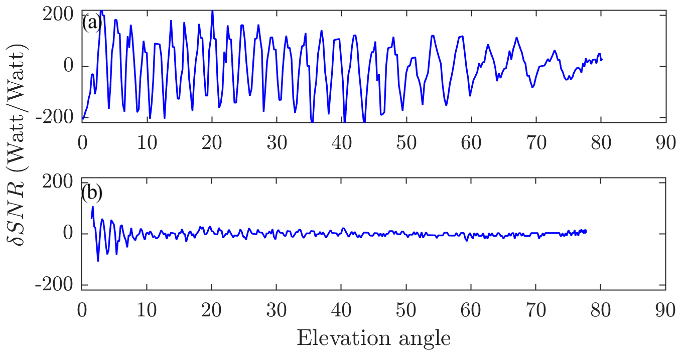
Figure 1Examples of the interference pattern observed in detrended SNR data as a function of satellite elevation angle for (a) one of the GNSS100L antennas used in this study placed approximately 3 m above a water surface and (b) a Leica AR25 antenna at site GTGU in Onsala, Sweden, situated approximately 4 m above a water surface. The data for site GTGU are available online as part of the study Geremia-Nievinski et al. (2020). The oscillations in (b) are dampened with increasing elevation angle, whereas in (a) the oscillations have a constant amplitude.
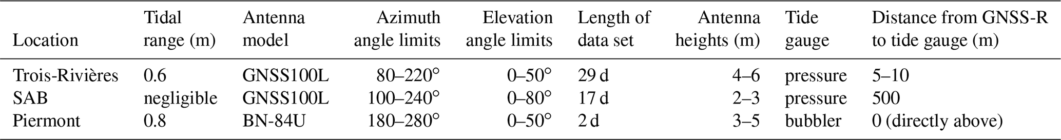
Our experimental antenna arrays were tested at two locations along the Saint Lawrence River in Quebec, Canada, and one location on the Hudson River in Piermont, NY, USA. Pictures of the three installations are given in Fig. 2. There is a water level sensor at each site near to where the antennas were installed. For disambiguation, we will refer to these water level sensors as tide gauges henceforth. The Saint Lawrence River is an ideal testing ground in that water level variations are forced by a range of different signals. From Lake Ontario to the island of Montréal water level variations are dominated by drainage of precipitation, seasonal snow melt and dam activity, whilst tidal forcing becomes progressively more dominant from Montréal to Québec City, where the estuary to the Atlantic Ocean begins. Daily water level variations at Piermont are also dominated by tides. Key information for the three sites used is summarised in Table 1. The azimuth and elevation angle limits correspond to the region from which the antenna is receiving reflected signals on the water surface and were determined based on visual inspection of oscillations in the SNR data.
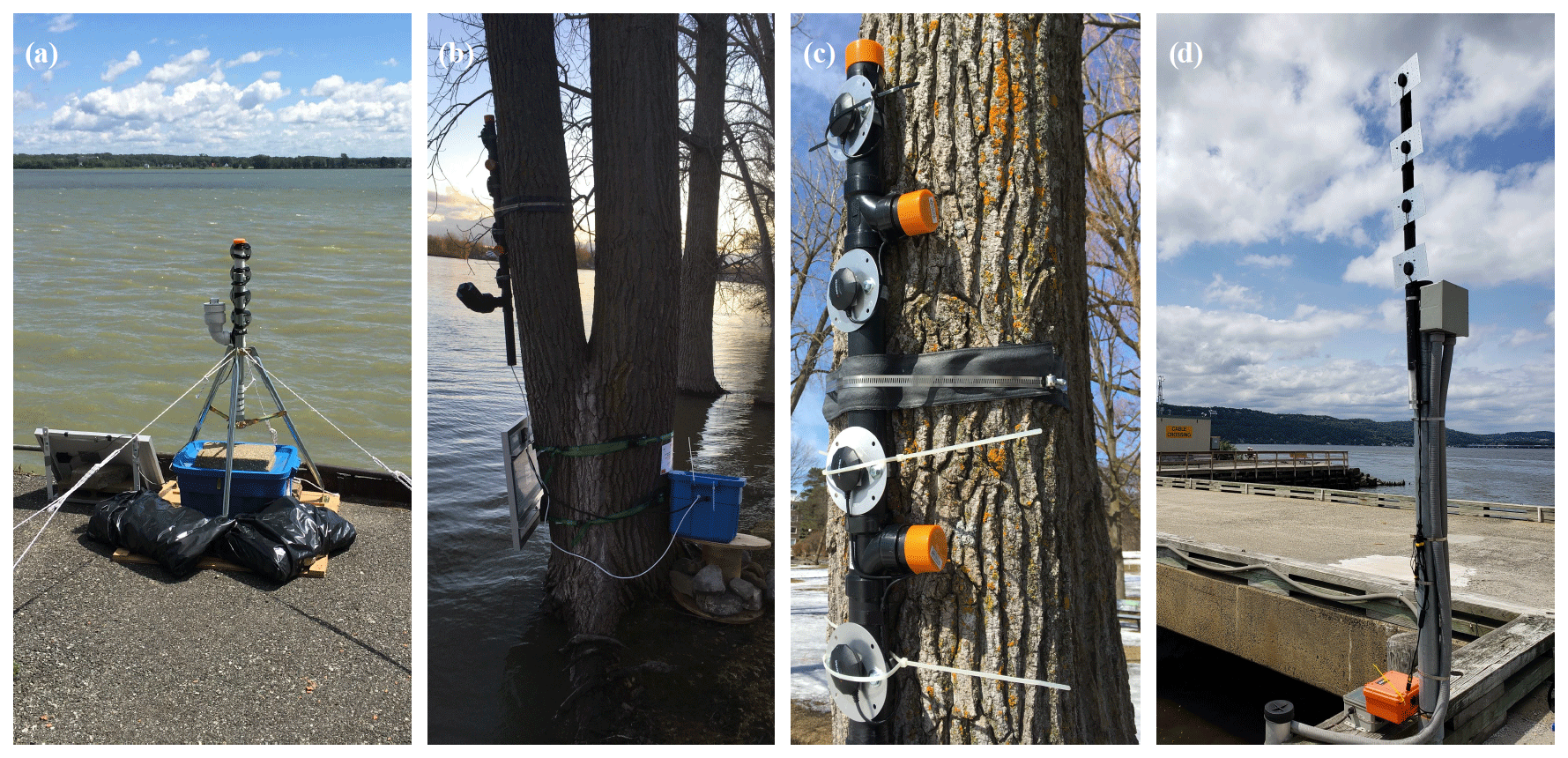
Figure 2Pictures of antenna arrays (a) at Trois-Rivières, (b) and (c) show different angles at Sainte-Anne-de-Bellevue and (d) at Piermont. The antenna array shown in (b) and (c) was also temporarily installed at Trois-Rivières. The antennas are closer together in (a) in comparison to the other two setups.
Table 1Information about the three test sites. “SAB” refers to Saint-Anne-de-Bellevue. Antenna heights refer to mean heights above the water surface.
The site at which we collected the longest continuous data set is at the Port of Trois-Rivières. This site is on the north shore of the Saint Lawrence River, west (upstream) of the confluence with the Saint Maurice River. Trois-Rivières is approximately midway between Montréal and Québec City; hence daily water level variations are dominated by tides. There are three OTT Hydromet pressure level sensors at this site. The average of water level measurements from the three sensors is provided at intervals of 3 min from the Canadian Hydrographic Service. According to the instrument handbook, the accuracy is 0.5 cm or less. The narrow GNSS100L antenna array collected data for a continuous 4-week period from 11 September to 9 October. Both narrow and wide GNSS100L antenna arrays were also installed for a 5 d period in August 2020. The antenna arrays at this site were installed approximately 5–10 m away from the tide gauges.
The second site in Quebec is in Sainte-Anne-de-Bellevue, at the western tip of the island of Montréal. The stretch of coast where the antennas were situated is part of the northern border of Lake Saint-Louis, which is at the meeting point of the Saint Lawrence and the Ottawa rivers. We installed the antennas on a tree looking over the lake (Fig. 2b). The antennas were installed between February and June 2020; however the lake was frozen for the first 2 months of this period, and the antennas were not continuously recording data due to logistical issues associated with the COVID-19 pandemic. Here we focus on a continuous period of data from 17 May to 2 June. We used data from a nearby Environment and Climate Change Canada tide gauge to validate our GNSS-R measurements. The tide gauge is a Campbell Scientific CS450 pressure transducer and data are available online at 6 min intervals from the Government of Canada. It is not clear what specific model of the CS450 sensor is installed at this site, but if we assume that it is a standard accuracy model with 10 m range, the accuracy is at most 1 cm. The tide gauge is situated approximately 500 m west of where the antenna array was installed, just south of a canal and the Sainte Anne Rapids that flow from the Lake of Two Mountains to Lake Saint-Louis (see Fig. 3). We are cautious because differences between the tide gauge and GNSS-R measurements at site could be partly accounted for by differences in the local flow regimes.
At the site on the Hudson River in New York, the antenna array was installed at the end of a large pier. The antennas were mounted on a pole directly above a Sutron constant-flow bubbler for an approximately 48 h period from 8–10 September 2020. Data from the bubbler tide gauge at intervals of 15 min was downloaded online from the United States Geological Survey. According to the instrument specifications, the accuracy of this sensor is approximately 0.3 cm (0.01 ft).
The RMSE between GNSS-R and tide gauge measurements is used henceforth as a proxy for the precision of the GNSS-R measurements. If we assume that errors from the tide gauge and GNSS-R measurements are not correlated, then the RMSE is actually an upper limit for the precision. It is not a focus of this study to calculate the datum of the GNSS-R measurements relative to that of the tide gauges; hence the mean is removed from each time series and the RMSE is then calculated by evaluating the b-spline curve from inverse modelling at each time that a measurement from the tide gauge exists.
The GNSS-R water level measurements obtained using inverse modelling of SNR data from four low-cost antennas are plotted alongside tide gauge measurements at all three sites in Fig. 4. There is a good agreement between the GNSS-R and tide gauge measurements at all sites; for the 29 d period at Trois-Rivières the RMSE is 1.02 cm, for the 17 d period at Sainte-Anne-de-Bellevue the RMSE is 0.69 cm, and for the 2 d period at Piermont the RMSE is 1.16 cm. To help visualise the data that are obtained from the arrays of four antennas, an example of the reflector height solutions from each antenna at Sainte-Anne-de-Bellevue is given in Fig. 5. There is also a shorter period of data for each site plotted with GNSS-R minus tide gauge measurement residuals given in Fig. S1.
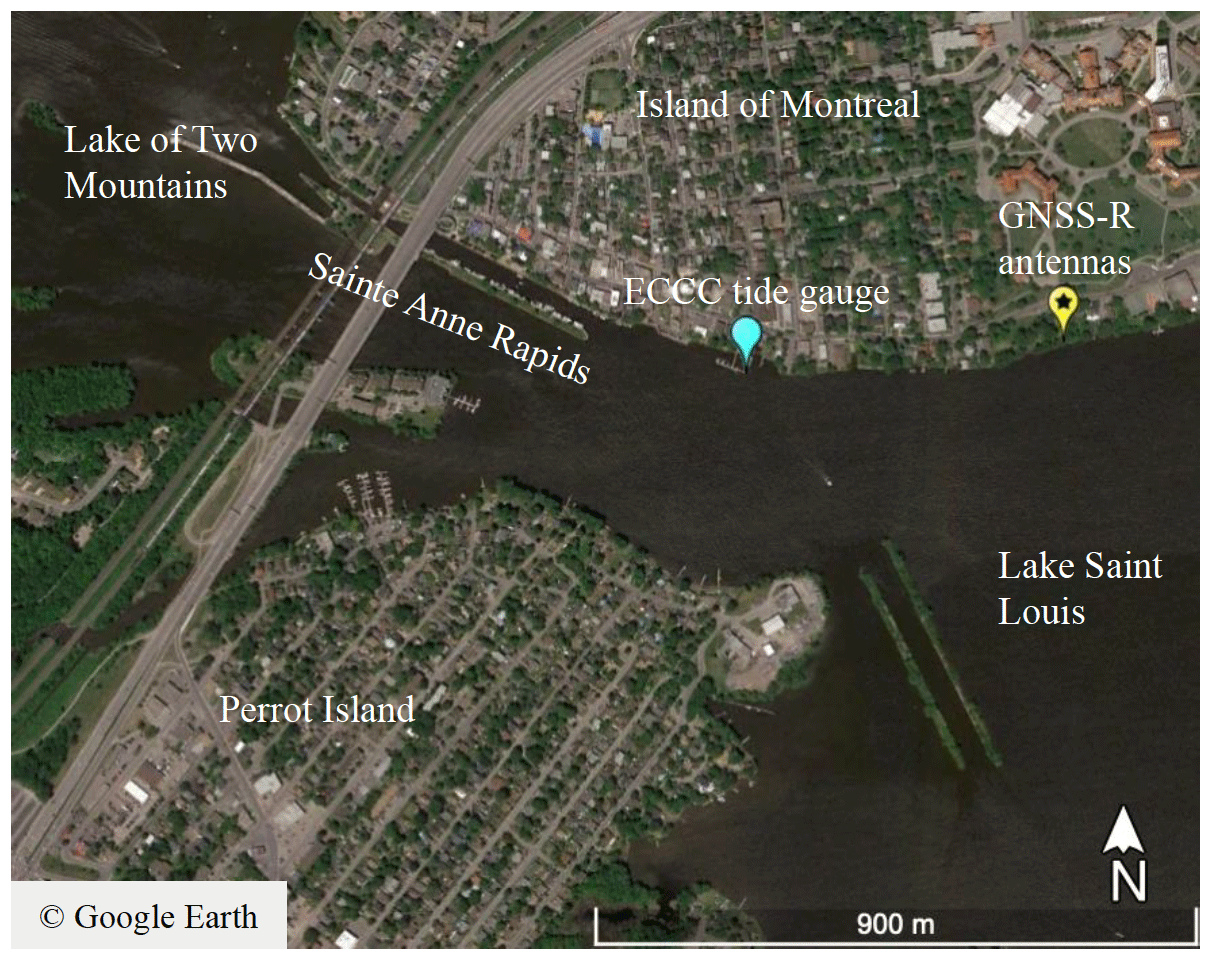
Figure 3The area surrounding the antenna array and tide gauge at Sainte-Anne-de-Bellevue.
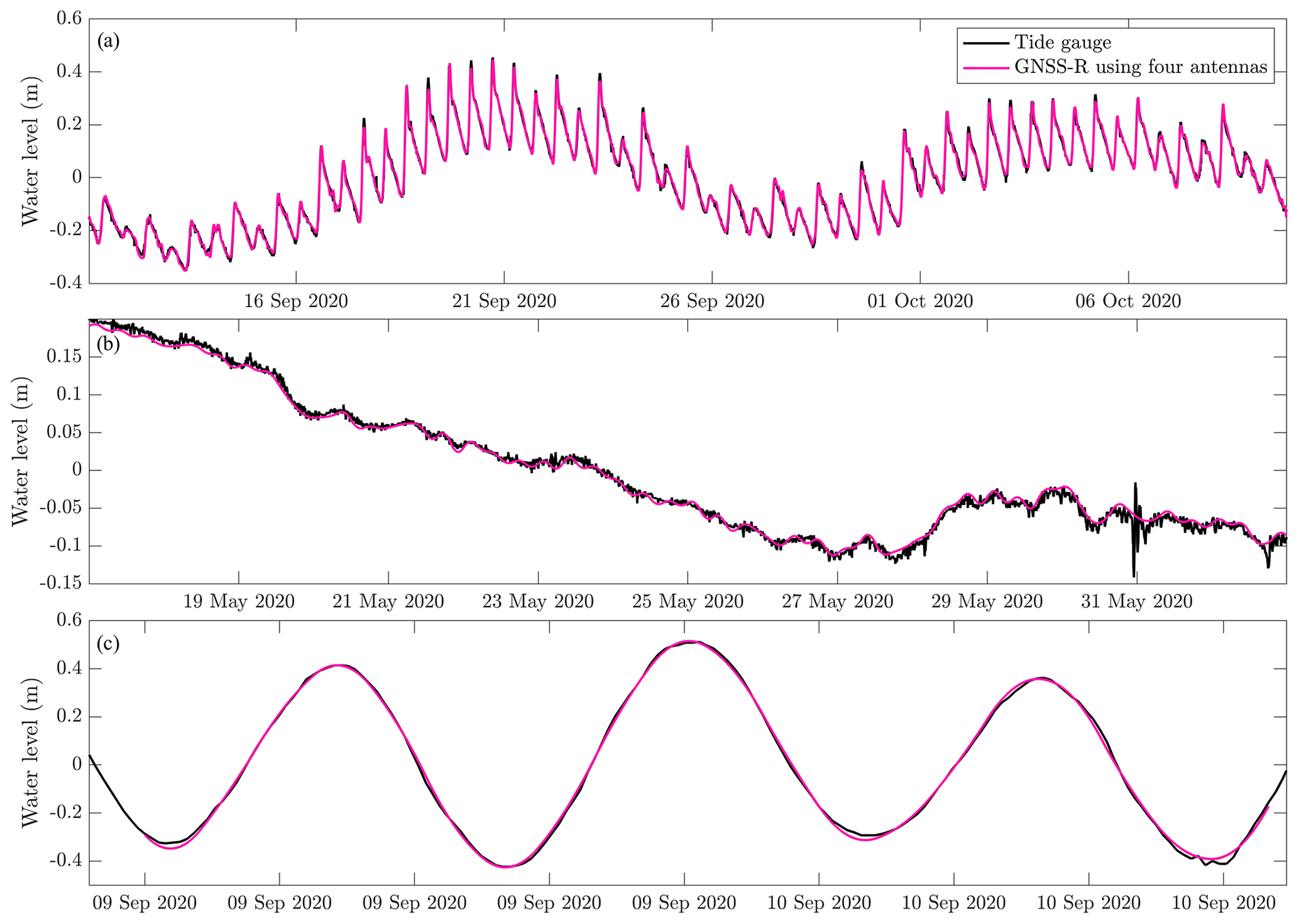
Figure 4A comparison of GNSS-R and tide gauge measurements at (a) Trois-Rivières, (b) Sainte-Anne-de-Bellevue and (c) Piermont. The mean of each time series is removed before plotting.

Figure 5Reflector height measurements from four antennas at Sainte-Anne-de-Bellevue. The solid lines represent the b-spline solutions from inverse modelling and the dots are estimates from spectral analysis. The b-spline parameters that are used to plot the solid lines in this figure are averaged to form the single solution in Fig. 4b. The curves are inverted because reflector height increases as water level decreases.
The daily water level variations at Trois-Rivières (in Fig. 4a) and Piermont (in Fig. 4c) are dominated by the principal lunar semidiurnal tides. However, tidal waves are modified in the shallow river channel at Trois-Rivières such that the crests travel faster than the troughs, which gives rise to the sawtooth-like pattern at Trois-Rivières as opposed to the smoothly varying sinusoid that dominates the signal at Piermont. Daily water level variations at Sainte-Anne-de-Bellevue (in Fig. 4b) are of much smaller magnitude as there are negligible tides. The water level variations at this site are driven by drainage of precipitation and other hydrological effects, for example it rained upstream of Montréal on 28 May, which corresponds with a rise in the observed water level on this day at Sainte-Anne-de-Bellevue.
5.1 Influence of multiple co-located antennas
There is an improvement in the precision of water level measurements when using four antennas as opposed to using just one antenna at all three sites. Reading values from Table 2, if the RMSE obtained with four antennas is compared to the maximum RMSE obtained with one antenna, there is a reduction of 1.23 cm (or 50 %) at Trois-Rivières, 0.26 cm (or 30 %) at Sainte-Anne-de-Bellevue and 0.51 cm (or 30 %) at Piermont. The results from Table 2 indicate a significant improvement (up to 0.62 cm) when using four instead of two antennas, but minimal improvement between three and four antennas. Having four antennas is also recommended over three antennas in case of redundancy. Note that whilst the difference between the minimum RMSE obtained with one antenna is comparable to that obtained with four antennas, our analysis suggests that the relative performance of each antenna appears to be random, which in turn implies that the upper limit should be used for comparison. For example, if the data from Trois-Rivières are split into two 2-week periods and analysed separately, the antennas that give the most and least precise results are not the same for both periods, and neither of these sets in turn match those for the total 4-week period.
Table 2Summary of results obtained using different combinations of antennas to retrieve water level measurements. For one to three antennas, the RMSE for every combination of antennas at each site was calculated, but only the lowest and highest values are shown in the table.

During a period of 4 d, we performed an experiment with two arrays of four antennas (eight in total) installed at different heights and found that there is no advantage in installing more than four antennas at the same site. For this 4 d period there is an RMSE of 1.06 cm when using just the narrow configuration, 1.32 cm when using just the wide configuration, or 1.14 cm when using both narrow and wide simultaneously. Given that the configurations were installed several metres apart, we tested different combinations of antennas across both configurations to see if the spacing of antennas influences the precision when using multiple antennas and found that there is no advantage in using antennas spaced further apart than the narrow configuration. These findings together with our analyses at all three sites also indicate that there is no clear dependence on the heights of the antennas above the water surface. These results also suggest that the source of noise in the SNR data is likely due to random instrument noise as opposed to interference from the local environment.
Our results so far have focused on inverse modelling of SNR data, but spectral analysis estimates, shown as dots in Fig. 5, can also be compared with the tide gauge measurements. The RMSE of hourly means of spectral analysis estimates at Sainte-Anne-de-Bellevue varies from 2.40–3.90 cm for each antenna. The hourly means can then be combined into a single time series by removing the height offset from each antenna and taking the median of the hourly values, which gives an RMSE of 1.94 cm. The maximum improvement of 1.96 cm when using four antennas as opposed to a single antenna for spectral analysis estimates is much larger than the 0.26 cm maximum improvement when using inverse modelling at this site. These differences between inverse modelling and spectral analysis suggest that random noise is a larger source of uncertainty when using spectral analysis, thus supporting the results from Purnell et al. (2020). These results demonstrate that using multiple antennas in the same location is an effective technique for improving the precision in GNSS-R water level measurements, regardless of the technique that is used.
The results described above were obtained after exploring a large parameter space related to the inverse modelling and experimental setup. The most important parameters to consider are the elevation angle limits, the azimuth angle limits, the b-spline knot spacing and time window length, the satellite constellations used, and the temporal resolution of data. We discuss the results of tests with these parameters below. The results discussed in this section were all obtained using the inverse modelling technique given in Sect. 2.
Note that elevation and azimuth angle limits are constrained by the site surroundings, and the discussions in Sect. 6.2 and 6.1 refer to investigating optimal limits within these pre-defined constraints. A given azimuth and elevation angle corresponds to a Fresnel zone on the reflecting surface where the power of the signal is concentrated. Software for calculating and visualising Fresnel zones is given by Roesler and Larson (2018). As the elevation angle decreases, the Fresnel zone increases in size and moves away from the antenna, whereas changing the azimuth angle rotates the Fresnel zone laterally around the antenna. The limits given in Table 1 correspond roughly to the region in which the Fresnel zones are on the water surface and where there are no objects obstructing the view of the water surface (e.g. moored boats).
6.1 Elevation angle limits
Using low-cost antennas we retrieved water level measurements over a range of elevation angles up to 50∘ at Trois-Rivières and Piermont and up to 80∘ at Sainte-Anne-de-Bellevue, whereas previous ground-based GNSS-R studies have been limited to the use of elevation angles up to 35∘. Due to a number of trade-offs between low and high elevation angles, we found optimal limits of 10–50∘ at all three sites. For sites located at midlatitudes to high latitudes (such as our sites), satellites are more prevalent towards the Equator (i.e. to the south of our instruments) at lower elevation angles, and therefore using lower elevation angles increases the amount of SNR data that is available for analysis. We find that reflector height measurements are generally less precise at elevation angles greater than 30∘, in agreement with previous work using geodetic-standard antennas that found the effect of random noise in SNR data leads to a greater uncertainty at larger elevation angles (Purnell et al., 2020). However, the effect of tropospheric delay increases with decreasing elevation angle and leads to an underestimation of the reflector height (Williams and Nievinski, 2017). For our sites, tropospheric delay has a minor effect on the precision, but aforementioned literature (e.g. Nikolaidou et al., 2020) suggests that this effect is more important at sites where the antennas are at a greater height above the water surface (e.g. >5 m) or where there is a large tidal range (e.g. >2 m) and especially when attempting to find the datum of reflector height measurements (not done here). In general, we find that it is most important to use a large range of elevation angles (e.g. 30∘ or more) to eliminate any gaps in time in the SNR data, and this is especially important at sites with daily tidal variations, such as at Trois-Rivières and Piermont. We initially tried to use a lower limit of 20∘, where the effect of tropospheric delay becomes negligible (Nikolaidou et al., 2020) but found more precise measurements using a lower limit of 10∘ at Trois-Rivières and Piermont. Limits of 20–50∘ can be used to make equally precise measurements as 10–50∘ at Sainte-Anne-de-Bellevue.
6.2 Azimuth angle limits
In general, azimuth angle limits should be fixed to match the widest unobstructed view of the water surface. In contrast with elevation angles, there are no complicated azimuth-angle-dependent effects; the larger the range of azimuth angle limits, the more data for GNSS-R analysis. The only complicating factor is that some azimuth angles yield more data per day than others because satellites are more prevalent towards the south at midlatitudes to high latitudes in the Northern Hemisphere or vice versa in the Southern Hemisphere. To demonstrate the importance of maximising the azimuth angle range, we retrieved water level measurements at Trois-Rivières and Sainte-Anne-de-Bellevue with the azimuth angle range reduced from 140 to 100∘. The RMSE increased by approximately 50 % (from 1.02 to 1.49 cm) at Trois-Rivières and 15 % (from 0.69 to 0.79 cm) at Sainte-Anne-de-Bellevue when using the reduced azimuth angle ranges.
6.3 B-spline knot spacing and time window
For the results described in the previous section, the b-spline knot spacing and time window length vary for each site: at Trois-Rivières we use a knot spacing of 1 h and a time window of 6 h, at Sainte-Anne-de-Bellevue we use a knot spacing of 4 h and a time window of 24 h, and at Piermont we use a knot spacing of 2 h and a time window of 6 h. In general, the knot spacing should be set to 1 h at a site with large daily tidal variations or a site with a complicated signal (such as the sawtooth-like signal at Trois-Rivières). Note that there is automatically a lower limit on the precision that can be achieved using inverse modelling because a b-spline curve cannot perfectly represent the time series. This lower limit on the precision increases with increasing knot spacing. For example, if we directly fit a b-spline curve to the tide gauge measurements at Trois-Rivières shown in Fig. 4a, we find an RMSE of 0.5 cm if using a knot spacing of 1 h or 1.6 cm if using a knot spacing of 2 h. However, decreasing the knot spacing for inverse modelling also decreases the amount of SNR data that is used to compute each b-spline scaling factor, potentially leading to less precise results; hence we do not recommend using a knot spacing of less than 1 h.
The time window should be at least 3 times the length of the knot spacing. Provided that this minimum is met, the length of the time window does not appear to impact the precision in our experiments. However, both increasing the window length or decreasing the knot spacing greatly increases the computation time for the inverse modelling.
6.4 Satellite constellations
Using data simultaneously from all three satellite constellations that are tracked by our low-cost antennas (GPS, GLONASS and Galileo) is important to achieve the most precise results. For example, when using only GPS data at Trois-Rivières, the RMSE increases by over 200 % compared to the results obtained using all three constellations (the RMSE is 3.11 cm with just GPS compared to 1.02 cm with all three constellations). Using any combination of two constellations also leads to less precise results than using all three constellations: the RMSE increases by approximately 30 % (to 1.27 cm) when using just GPS and GLONASS together or 170 % (to 2.69 cm) when using just GLONASS and Galileo together. It is not clear if these differences are due to the prevalence of satellites (there are more GPS satellites) or differences in the signals themselves.
6.5 Temporal resolution of SNR data
The temporal resolution of SNR data greatly affects the computation time for inverse modelling. Data were recorded at our sites every second but we found that it was most efficient to resample the data to intervals of 15 s prior to analysis. When varying the temporal resolution between 1 and 15 s at Trois-Rivières, we found that the RMSE varies by less than 1 mm but the computation time increases greatly when using an interval time of 1 s. The RMSE increases by approximately 70 % when decimating the data to intervals of 30 or 60 s. Recording data at intervals of 5, 10 or 15 s is therefore advantageous for data storage and efficient analysis. It is important to note, however, that the temporal resolution provides a limitation on the maximum reflector height that can be resolved due to the Nyquist frequency. See Roesler and Larson (2018) for a discussion on this Nyquist limit.
We presented a technique for retrieving precise water level measurements using arrays of four low-cost GNSS antennas and validated our technique at three sites with variable tidal forcing. By comparing it with nearby operational tide gauges, we found an upper limit on the precision of water level measurements of 0.69–1.16 cm at all sites, whereas previous studies using geodetic-standard antennas have found an RMSE of 2–50 cm. The RMSE values obtained are likely upper limits on the precision because they also contain error from the tide gauge measurements. The amount of error from the tide gauge measurements is also likely to differ between sites because there are different types of instruments at the sites in Quebec (pressure transducers) and Piermont (bubbler gauge). While pressure transducers are more susceptible to errors over multi-year timescales due to instrument drift (Míguez et al., 2005; Pytharouli et al., 2018), bubbler gauges are more susceptible to errors during wavy conditions (Woodworth and Smith, 2003). The results presented here are significant in that an accuracy of 1 cm is the benchmark set by GLOSS (2012) for studying multi-year trends in sea level. We found an improvement in the precision of 30 %–50 % when using four co-located antennas instead of one, which suggests that random noise is one of the key sources of uncertainty in GNSS-R measurements and supports the results from Purnell et al. (2020). In addition to the reduction in cost (on the order of several thousand USD or more), we found that the low-cost antennas are better suited for reflectometry than geodetic-standard antennas because they can be used to obtain water level measurements over a much larger range of elevation angles.
Our results provide a strong proof of concept, but work remains to be done to further validate and improve our technique. Most importantly, an array of antennas should be installed with a co-located tide gauge for a longer time period (e.g. for at least several months) and at a site with a larger tidal range. It is also necessary to attempt a levelling procedure so that the datum of the water level measurements can be defined. To place measurements on a global reference frame and simultaneously monitor local land deformation, an array of low-cost antennas could then be co-located with a geodetic-standard antenna with the aim of using the low-cost antennas to obtain precise water level measurements and the geodetic-standard antenna to perform precise positioning. More models of low-cost antennas should also be tested, preferably in the same location (we do not recommend one of the types of antennas used in this study over the other type because we have not had the opportunity to test them at the same location). Whilst our results suggest that the spacing apart of antennas is not important, we cannot rule out the possibility of interference between antennas at the separation distances used in this study. A rigorous investigation of the clearance distance required to ensure that antennas are not interfering should guide a future study. A vertical array of low-cost antennas such as those used in this study could be used to test the technique for obtaining high-rate sea level measurements recently proposed by Yamawaki et al. (2021).
For future installations of low-cost antennas, we propose the following guidelines:
-
at least four co-located antennas
-
the antennas should record data from GPS, GLONASS and Galileo satellites
-
the antennas should be positioned within 1–5 m above the water surface
-
the antennas should have an unobstructed view of the water surface that extends 140∘ or more laterally and at least 50 m outwards (this corresponds to the edge of the Fresnel zone for an antenna 5 m above the water surface and a satellite at 10∘ elevation)
-
data should be recorded at intervals of 5 s (or more, depending on the mean height of the antennas above the water surface and the associated Nyquist limit).
Upon obtaining data, the following inverse modelling parameters should be used to extract precise water level measurements:
-
a large range of elevation angles (e.g. 10–50∘)
-
a b-spline knot spacing of 1 h at a site with tides (or larger would be more efficient at a site with negligible tides)
-
a b-spline time window length of at least 3 times the knot spacing.
The above guidelines may be refined following further field work. For example, we found that having four antennas is optimal when we tested eight co-located antennas for a short period of 4 d – more data are needed to support this result. Additional data from other satellite constellations (such as BeiDou) and from other signals (such as L2C and L5) may also be useful.
Our technique for monitoring water levels with arrays of low-cost antennas could be applied to address the need for widespread, accessible water level measurements in the face of future climate change. The antenna arrays are relatively simple to build and therefore suited to citizen science efforts. They could be used to obtain sea level measurements in remote coastal regions as well as lake level or river stage measurements at a fraction of the cost of commercially available sensors but with comparable precision. Such measurements could be used to validate satellite measurements and to better constrain tidal models in the polar regions, where there are few coastal sea level measurements. A dense network of sensors could also be installed to detect spatially variable sea level signals, for example near tidewater glaciers to detect so-called sea level fingerprints (Mitrovica et al., 2011).
Codes for analysing low-cost GNSS data to produce water level measurements using MATLAB or Python software can be found at https://doi.org/10.5281/zenodo.4790412 (Purnell, 2021). There is also 1 d of sample data (the 13 September 2020) from the “narrow” antenna array at Trois-Rivières contained in this repository.
The supplement related to this article is available online at: https://doi.org/10.5194/esurf-9-673-2021-supplement.
DJP, NG and WM conceptualised the study. DJP performed analysis and wrote all codes to go along with the article. WM designed and built the initial low-cost antenna array (including software). GL, DJP and DP built subsequent antenna arrays and performed field work. DJP wrote the initial article draft and NG, WM and DP helped to improve the article.
The authors declare that they have no conflict of interest.
The authors would like to thank the Port of Trois-Rivières, the Canadian Hydrographic Service, Fisheries and Oceans Canada, and Environment and Climate Change Canada for help with field work and obtaining tide gauge data. We also thank Manuella Fagundes and an anonymous reviewer for comments that helped to improve the article. Codes were translated from MATLAB to Python with support from Claire Marie Guimond.
This research has been supported by the McGill University (The Trottier Fellowship for Science and Public Policy), the Fonds de recherche du Québec – Nature et technologies (New researchers programme), the McGill Space Institute (Graduate fellowship), the American Geophysical Union (Jerome M. Paros scholarship in geophysical instrumentation), and the Canada Research Chairs (Canada Research Chairs Program).
This paper was edited by Giulia Sofia and reviewed by Manuella Fagundes and one anonymous referee.
Adrian, R., O'Reilly, C. M., Zagarese, H., Baines, S. B., Hessen, D. O., Keller, W., Livingstone, D. M., Sommaruga, R., Straile, D., Van Donk, E., Weyhenmeyer, G. A., and Winder, M.: Lakes as sentinels of climate change, Limnol. Oceanogr., 54, 2283–2297, https://doi.org/10.4319/lo.2009.54.6_part_2.2283, 2009. a
Baumann, T. M., Polyakov, I. V., Padman, L., Danielson, S., Fer, I., Janout, M., Williams, W., and Pnyushkov, A. V.: Arctic tidal current atlas, Scientific Data, 7, 275, https://doi.org/10.1038/s41597-020-00578-z, 2020. a
Beckmann, P. and Spizzichino, A.: The scattering of electromagnetic waves from rough surfaces, Artech House, Norwood, MA, USA, 1987. a
Dullaart, J. C. M., Muis, S., Bloemendaal, N., and Aerts, J. C. J. H.: Advancing global storm surge modelling using the new ERA5 climate reanalysis, Clim. Dynam., 54, 1007–1021, https://doi.org/10.1007/s00382-019-05044-0, 2020. a
Fagundes, M. A. R., Mendonça-Tinti, I., Iescheck, A. L., Akos, D. M., and Geremia-Nievinski, F.: An open-source low-cost sensor for SNR-based GNSS reflectometry: design and long-term validation towards sea-level altimetry, GPS Solutions, 25, 73, https://doi.org/10.1007/s10291-021-01087-1, 2021. a, b, c
Geremia-Nievinski, F., Hobiger, T., Haas, R., Liu, W., Strandberg, J., Tabibi, S., Vey, S., Wickert, J., and Williams, S.: SNR-based GNSS reflectometry for coastal sea-level altimetry: results from the first IAG inter-comparison campaign, J. Geodesy, 94, 70, https://doi.org/10.1007/s00190-020-01387-3, 2020. a
GLOSS: Global Sea-Level Observing System (GLOSS) Implementation Plan, IOC Technical Series No. 100 (English), UNESCO/IOC, 2012. a, b, c
Goudie, A. S.: Global warming and fluvial geomorphology, Geomorphology, 79, 384–394, https://doi.org/10.1016/j.geomorph.2006.06.023, 2006. a
Gómez-Enri, J., Vignudelli, S., Cipollini, P., Coca, J., and González, C.: Validation of CryoSat-2 SIRAL sea level data in the eastern continental shelf of the Gulf of Cadiz (Spain), Adv. Space Res., 62, 1405–1420, https://doi.org/10.1016/j.asr.2017.10.042, 2018. a
Khan, S. A., Bjørk, A. A., Bamber, J. L., Morlighem, M., Bevis, M., Kjær, K. H., Mouginot, J., Løkkegaard, A., Holland, D. M., Aschwanden, A., Zhang, B., Helm, V., Korsgaard, N. J., Colgan, W., Larsen, N. K., Liu, L., Hansen, K., Barletta, V., Dahl-Jensen, T. S., Søndergaard, A. S., Csatho, B. M., Sasgen, I., Box, J., and Schenk, T.: Centennial response of Greenland's three largest outlet glaciers, Nat. Commun., 11, 5718, https://doi.org/10.1038/s41467-020-19580-5, 2020. a
Kopp, R. E., Hay, C. C., Little, C. M., and Mitrovica, J. X.: Geographic Variability of Sea-Level Change, Current Climate Change Reports, 1, 192–204, https://doi.org/10.1007/s40641-015-0015-5, 2015. a
Larson, K. M., Ray, R. D., Nievinski, F. G., and Freymueller, J. T.: The Accidental Tide Gauge: A GPS Reflection Case Study From Kachemak Bay, Alaska, IEEE Geosci. Remote S., 10, 1200–1204, https://doi.org/10.1109/LGRS.2012.2236075, 2013. a, b, c
Meyssignac, B., Slangen, A. B. A., Melet, A., Church, J. A., Fettweis, X., Marzeion, B., Agosta, C., Ligtenberg, S. R. M., Spada, G., Richter, K., Palmer, M. D., Roberts, C. D., and Champollion, N.: Evaluating Model Simulations of Twentieth-Century Sea-Level Rise. Part II: Regional Sea-Level Changes, J. Climate, 30, 8565–8593, https://doi.org/10.1175/JCLI-D-17-0112.1, 2017. a
Mitrovica, J. X., Gomez, N., Morrow, E., Hay, C., Latychev, K., and Tamisiea, M. E.: On the robustness of predictions of sea level fingerprints, Geophys. J. Int., 187, 729–742, https://doi.org/10.1111/j.1365-246X.2011.05090.x, 2011. a
Míguez, B. M., Gómez, B. P., and Fanjul, E. A.: The ESEAS-RI Sea Level Test Station: Reliability and Accuracy of Different Tide Gauges, The International Hydrographic Review, 6, 44–53, 2005. a, b, c
Nikolaidou, T., Santos, M. C., Williams, S. D. P., and Geremia-Nievinski, F.: Raytracing atmospheric delays in ground-based GNSS reflectometry, J. Geodesy, 94, 68, https://doi.org/10.1007/s00190-020-01390-8, 2020. a, b, c, d
Pattyn, F. and Morlighem, M.: The uncertain future of the Antarctic Ice Sheet, Science, 367, 1331–1335, https://doi.org/10.1126/science.aaz5487, 2020. a
Peng, F. and Deng, X.: Validation of Sentinel-3A SAR mode sea level anomalies around the Australian coastal region, Remote Sens. Environ., 237, 111548, https://doi.org/10.1016/j.rse.2019.111548, 2020. a
Purnell, D., Gomez, N., Chan, N. H., Strandberg, J., Holland, D. M., and Hobiger, T.: Quantifying the Uncertainty in Ground-Based GNSS-Reflectometry Sea Level Measurements, IEEE J. Sel. Top. Appl., 13, 4419–4428, https://doi.org/10.1109/JSTARS.2020.3010413, 2020. a, b, c, d, e
Purnell, D.: gnssr_lowcost, https://doi.org/10.5281/zenodo.4790412, 2021. a
Pytharouli, S., Chaikalis, S., and Stiros, S. C.: Uncertainty and bias in electronic tide-gauge records: Evidence from collocated sensors, Measurement, 125, 496–508, https://doi.org/10.1016/j.measurement.2018.05.012, 2018. a, b, c
Roesler, C. and Larson, K. M.: Software tools for GNSS interferometric reflectometry (GNSS-IR), GPS Solutions, 22, 80, https://doi.org/10.1007/s10291-018-0744-8, 2018. a, b
Santamaría-Gómez, A. and Watson, C.: Remote leveling of tide gauges using GNSS reflectometry: case study at Spring Bay, Australia, GPS Solutions, 21, 451–459, https://doi.org/10.1007/s10291-016-0537-x, 2017. a, b
Seifi, F., Deng, X., and Andersen, O. B.: Assessment of the Accuracy of Recent Empirical and Assimilated Tidal Models for the Great Barrier Reef, Australia, Using Satellite and Coastal Data, Remote Sens., 11, 1211, 2019. a
Sermet, Y., Villanueva, P., Sit, M. A., and Demir, I.: Crowdsourced approaches for stage measurements at ungauged locations using smartphones, Hydrolog. Sci. J., 65, 813–822, https://doi.org/10.1080/02626667.2019.1659508, 2020. a
Slangen, A. B. A., Church, J. A., Agosta, C., Fettweis, X., Marzeion, B., and Richter, K.: Anthropogenic forcing dominates global mean sea-level rise since 1970, Nat. Clim. Change, 6, 701–705, https://doi.org/10.1038/nclimate2991, 2016. a
Strandberg, J. and Haas, R.: Can We Measure Sea Level With a Tablet Computer?, IEEE Geosci. Remote S., 17, 1–3, 2019. a, b
Strandberg, J., Hobiger, T., and Haas, R.: Improving GNSS-R sea level determination through inverse modeling of SNR data, Radio Sci., 51, 1286–1296, https://doi.org/10.1002/2016RS006057, 2016. a, b, c, d, e, f
Tabibi, S., Nievinski, F. G., Dam, T. V., and Monico, J. F.: Assessment of modernized GPS L5 SNR for ground-based multipath reflectometry applications, Adv. Space Res., 55, 1104–1116, https://doi.org/10.1016/j.asr.2014.11.019, 2015. a
Tabibi, S., Geremia-Nievinski, F., Francis, O., and van Dam, T.: Tidal analysis of GNSS reflectometry applied for coastal sea level sensing in Antarctica and Greenland, Remote Sens. Environ., 248, 111959, https://doi.org/10.1016/j.rse.2020.111959, 2020. a, b, c
Taherkhani, M., Vitousek, S., Barnard, P. L., Frazer, N., Anderson, T. R., and Fletcher, C. H.: Sea-level rise exponentially increases coastal flood frequency, Sci. Rep., 10, 6466, https://doi.org/10.1038/s41598-020-62188-4, 2020. a
Tamisiea, M. E., Hughes, C. W., Williams, S. D. P., and Bingley, R. M.: Sea level: measuring the bounding surfaces of the ocean, Philosophical Transactions of the Royal Society A: Mathematical, Phys. Eng. Sci., 372, 20130336, https://doi.org/10.1098/rsta.2013.0336, 2014. a
Williams, S. D. P. and Nievinski, F. G.: Tropospheric delays in ground-based GNSS multipath reflectometry–Experimental evidence from coastal sites, J. Geophsy. Res.-Sol., 122, 2310–2327, https://doi.org/10.1002/2016JB013612, 2017. a, b, c
Williams, S. D. P., Bell, P. S., McCann, D. L., Cooke, R., and Sams, C.: Demonstrating the Potential of Low-Cost GPS Units for the Remote Measurement of Tides and Water Levels Using Interferometric Reflectometry, J. Atmos. Ocean. Technol., 37, 1925–1935, https://doi.org/10.1175/JTECH-D-20-0063.1, 2020. a, b, c
Woodworth, P. L. and Smith, D. E.: A One Year Comparison of Radar and Bubbler Tide Gauges at Liverpool, The International Hydrographic Review, 4, available at: https://journals.lib.unb.ca/index.php/ihr/article/view/20630 (last access: 12 November 2019), 2003. a, b
Yamawaki, M. K., Geremia-Nievinski, F., and Monico, J. F. G.: High-Rate Altimetry in SNR-Based GNSS-R: Proof-of-Concept of a Synthetic Vertical Array, IEEE Geosci. Remote S., 1–5, https://doi.org/10.1109/LGRS.2021.3068091, 2021. a