Higher sediment redistribution rates related to burrowing animals than previously assumed as revealed by time-of-flight-based monitoring

Burrowing animals influence surface microtopography and hillslope sediment redistribution, but changes often remain undetected due to a lack of automated high-resolution field monitoring techniques. In this study, we present a new approach to quantify microtopographic variations and surface changes caused by burrowing animals and rainfall-driven erosional processes applied to remote field plots in arid and Mediterranean climate regions in Chile. We compared the mass balance of redistributed sediment between burrow and burrow-embedded area, quantified the cumulative sediment redistribution caused by animals and rainfall, and upscaled the results to a hillslope scale. The newly developed instrument, a time-of-flight camera, showed a very good detection accuracy. The animal-caused cumulative sediment excavation was 14.6 cm³ cm⁻² yr⁻¹ in the Mediterranean climate zone and 16.4 cm³ cm⁻² yr⁻¹ in the arid climate zone. The rainfall-related cumulative sediment erosion within burrows was higher (10.4 cm³ cm⁻² yr⁻¹) in the Mediterranean climate zone than the arid climate zone (1.4 cm³ cm⁻² yr⁻¹). Daily sediment redistribution during rainfall within burrow areas was up to 350 %(40 %) higher in the Mediterranean (arid) zone compared to burrow-embedded areas and much higher than previously reported in studies that were not based on continuous microtopographic monitoring. A total of 38 % of the sediment eroding from burrows accumulated within the burrow entrance, while 62 % was incorporated into hillslope sediment flux, which exceeds previous estimations 2-fold. On average, animals burrowed between 1.2–2.3 times a month, and the burrowing intensity increased after rainfall. This revealed a newly detected feedback mechanism between rainfall, erosion, and animal burrowing activity, likely leading to an underestimation of animal-triggered hillslope sediment flux in wetter climates. Our findings hence show that the rate of sediment redistribution due to animal burrowing is dependent on climate and that animal burrowing plays a larger than previously expected role in hillslope sediment redistribution. Subsequently, animal burrowing activity should be incorporated into soil erosion and landscape evolution models that rely on soil processes but do not yet include animal-induced surface processes on microtopographical scales in their algorithms.

1 Introduction

Animal burrowing activity affects surface microtopography (Reichman and Seabloom, 2002; Kinlaw and Grasmueck, 2012), surface roughness (Yair, 1995; Jones et al., 2010; Hancock and Lowry, 2021), and soil physical properties (Ridd, 1996; Yair, 1995; Hall et al., 1999; Reichman and Seabloom, 2002; Hancock and Lowry, 2021; Coombes, 2016; Larsen et al., 2021; Corenblit et al., 2021). Previous studies estimated both positive and negative impacts of burrowing animals on sediment redistribution rates. These studies relied on applying tests under laboratory conditions using rainfall simulators; conducting several field campaigns weeks to months apart; or measuring the volume of excavated or eroded sediment in the field using instruments such as erosion pins, splash boards, or simple rulers (Imeson and Kwaad, 1976; Reichman and Seabloom, 2002; Wei et al., 2007; Le Hir et al., 2007; Li et al., 2018; T. C. Li et al., 2019; T. Li et al., 2019; Voiculescu et al., 2019; Chen et al., 2021; Übernickel et al., 2021b; G. Li et al., 2019). Although burrowing animals are generally seen as ecosystem engineers (Gabet et al., 2003; Wilkinson et al., 2009), their role in soil erosion in general, and for numerical soil erosion models in particular, is to date limited to predictions of burrow locations and particle mixing (Black and Montgomery, 1991; Meysman et al., 2003; Yoo et al., 2005; Schiffers et al., 2011). The complex interaction of sediment excavation and accumulation and erosion processes at the burrow and hillslope scale are not yet included in Earth surface models.

The reason for this knowledge gap is that previous studies have not provided data on low-magnitude but frequently occurring sediment redistribution due to a lack of spatiotemporal high-resolution microtopographic surface monitoring techniques that can also measure continuously in the field. Field experiments with, for example, rainfall simulators can unveil processes but cannot cover the time-dependent natural dynamics of sediment redistribution. When using erosion pins or splash boards, the sites had to be revisited each time, and the data were thus obtained only sporadically (Imeson and Kwaad, 1976; Hazelhoff et al., 1981; Richards and Humphreys, 2010). This limited all previous studies in their explanatory power because biotic-driven processes are typically characterized by their small quantity and frequent re-occurrence (Larsen et al., 2021). It is hence likely that previous studies based on non-continuously conducted measurements or rainfall experiments underestimated the role of burrowing animals on rates of hillslope sediment flux.

High-resolution, ground-based imaging sensing techniques have the potential to overcome limitations of previous surface monitoring techniques. Terrestrial laser scanner systems have been shown to be a suitable tool for the estimation of sediment redistribution and erosion processes (Nasermoaddeli and Pasche, 2008; Afana et al., 2010; Eltner et al., 2016b, a; Longoni et al., 2016). However, these instruments are expensive and labor intensive. Hence, a simultaneous, continuous, and automated monitoring of several animal burrows is for this reason not possible. Time-lapse photogrammetry is a low-cost (up to USD 5000) topographic monitoring technique, that can be applied at variable observation distances and scales (e.g., James and Robson, 2014; Galland et al., 2016; Eltner et al., 2017; Mallalieu et al., 2017; Kromer et al., 2019; Blanch et al., 2021). However, several cameras are needed to monitor the surface under various angles, which makes the field installation difficult and yields a large risk of disturbing the animals and leading to behavioral changes.

Another high-resolution surface monitoring technique is based on time-of-flight (ToF) technology. ToF-based cameras illuminate the targeted object with a light source for a known amount of time and then estimate the distance between the camera and the object by measuring the time needed for the reflected light to reach the camera sensor (Sarbolandi et al., 2018). ToF cameras exhibit lower spatial resolution and aerial coverage compared to time-lapse photogrammetry. However, the technique also has several advantages: as an active remote sensing tool it is able to monitor surface change at night, the processing is less complex compared to photogrammetry because the distance values are immediately received in a local coordinate system, and the field installation is much smaller and less invasive. ToF hence offers a new possibility for surface monitoring, as a technique for a cost-effective, high-resolution monitoring of sediment redistribution (Eitel et al., 2011; Hänsel et al., 2016), which can be achieved by a simple installation of only one device in the field.

In this study we developed, tested, and applied a cost-effective time-of-flight camera for automated monitoring of the rainfall and burrowing-animal-driven sediment redistribution of burrows and burrow-embedded areas with a high temporal (four times a day) and spatial (6 mm) resolution. For this, we equipped several plots at remote field study sites in the Chilean arid and Mediterranean climate zones. The selected field sites had a variable rainfall regime and sunlight exposure and were all affected by burrowing activity (Grigusova et al., 2021). After 7 months of field monitoring, including the wet and dry seasons, we estimated burrowing intensity and its dependence on rainfall. Following this, we quantified the daily sediment redistribution within the burrow and its embedding area, which enabled us to better understand the impacts of animal burrowing activity and rainfall on the local sediment redistribution. This allowed us to quantify the volume of burrow sediment that was incorporated into the hillslope sediment flux. Finally, we upscaled sediment redistribution rates to the entire hillslope.

2 Study area

Our study sites were located in the Chilean Coastal Cordillera in two climate zones (Fig. 1): in the National Park Pan de Azúcar (referred to hereafter as Pan de Azúcar or PdA) and the National Park La Campana (referred to hereafter as La Campana or LC). The Las Lomitas site at PdA is located in the arid climate zone of the Atacama Desert with a precipitation rate of 12 mm yr⁻¹, and it has a mean annual temperature of 16.8 ^∘C (Übernickel et al., 2021a). Here, the vegetation cover is below 5 %, and it is dominated by small desert shrubs, several species of cacti (Eulychnia breviflora, Copiapoa atacamensis) and biocrusts (Lehnert et al., 2018). LC is located in the Mediterranean climate zone, with a precipitation rate of 367 mm yr⁻¹ and a mean annual temperature of 14.1 ^∘C (Übernickel et al., 2021a). LC is dominated by an evergreen sclerophyllous forest with endemic palm trees (Jubaea chilensis). Both research sites have a granitic rock base, and the dominating soil texture is sandy loam (Bernhard et al., 2018). At PdA, the study setup consisted of one north-facing hillslope and one south-facing hillslope. The hillslope inclinations were ∼ 20^∘, and a climate station was located ∼ 15 km from the camera sites. At LC, the setup consisted of two north-facing hillslope and one south-facing hillslope. The hillslope inclinations were ∼ 25^∘, and a climate station was located ∼ 250 m from the south-facing hillslope (Übernickel et al., 2021a).

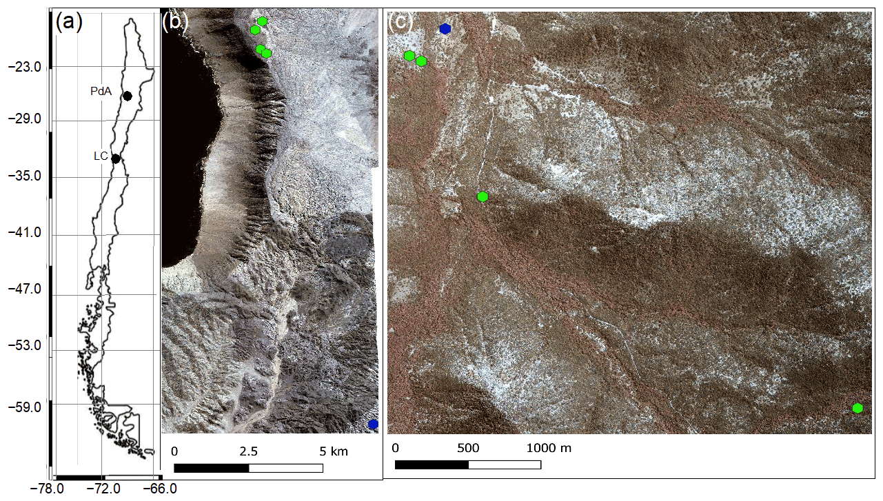
Figure 1 Location of the cameras and climate stations on which this study was based. Black points show the location of the research sites in Chile. The green points represent the camera plots, and the blue points the climate stations: (a) Location of study sites in Chile: PdA stands for Pan de Azúcar, and LC stands for La Campana. (b) Study setup in Pan de Azúcar. (c) Study setup at LC. The background images in (b) and (c) are orthophotos created from WorldView-2 data from 19 July 2019. For exact the latitude and longitude values, see Table A2.

2.1 Local burrowing animals

In order to assess which animal species burrowed at both study sites, we adapted a two-step approach. First, we used motion-activated camera traps to capture animals during the borrowing process at our field sites. Following this, we complemented the list of identified species with a literature review. We found that the most common vertebrate animal species that burrow at PdA were carnivores of the family Canidae (Lycalopex culpaeus, Lycalopex griseus) and rodents of the families Abrocomidae (Abrocoma bennetti), Chnichillidae (Lagidium viscacia), Cricetidae (Abrothrix andinus, Phyllotis xanthopygus, Phyllotis limatus, Phyllotis darwini), and Octogontidae (Cerquiera 1985; Jimenéz et al., 1992; Übernickel et al., 2021b) (Table 1). At LC, the most common burrowing vertebrate animal species were the carnivores of the family Canidae; Lagomorpha of the family Leporidae (Oryctolagus cuniculus); and rodents of the families Cricetidae (Abrothrix longipilis, Abrothrix olivaceus, Phyllotis darwini), Muridae (Mus musculus), and Octogontidae (Octodon degus, Spalacopus cyanus) (Munoz-Pedreros et al., 2018; Übernickel et al. 2021b) (Table 1). The motion-activated camera traps recorded several burrowing animals, all of which matched with the list of burrowing vertebrate animals collected from literature: Lycalopex culpaeus, Oryctolagus cuniculus, and Abrocoma bennettii (Fig. 2).

Table 1 The most common burrowing animals in the study sites. The list includes both animal species recorded with our motion-activated wildlife traps and those from the literature review (Übernickel et al. 2021; Cerquiera 1985; Jimenéz et al. 1992; Munoz-Pedreros et al. 2018); “×” indicates at which site the species can be found.

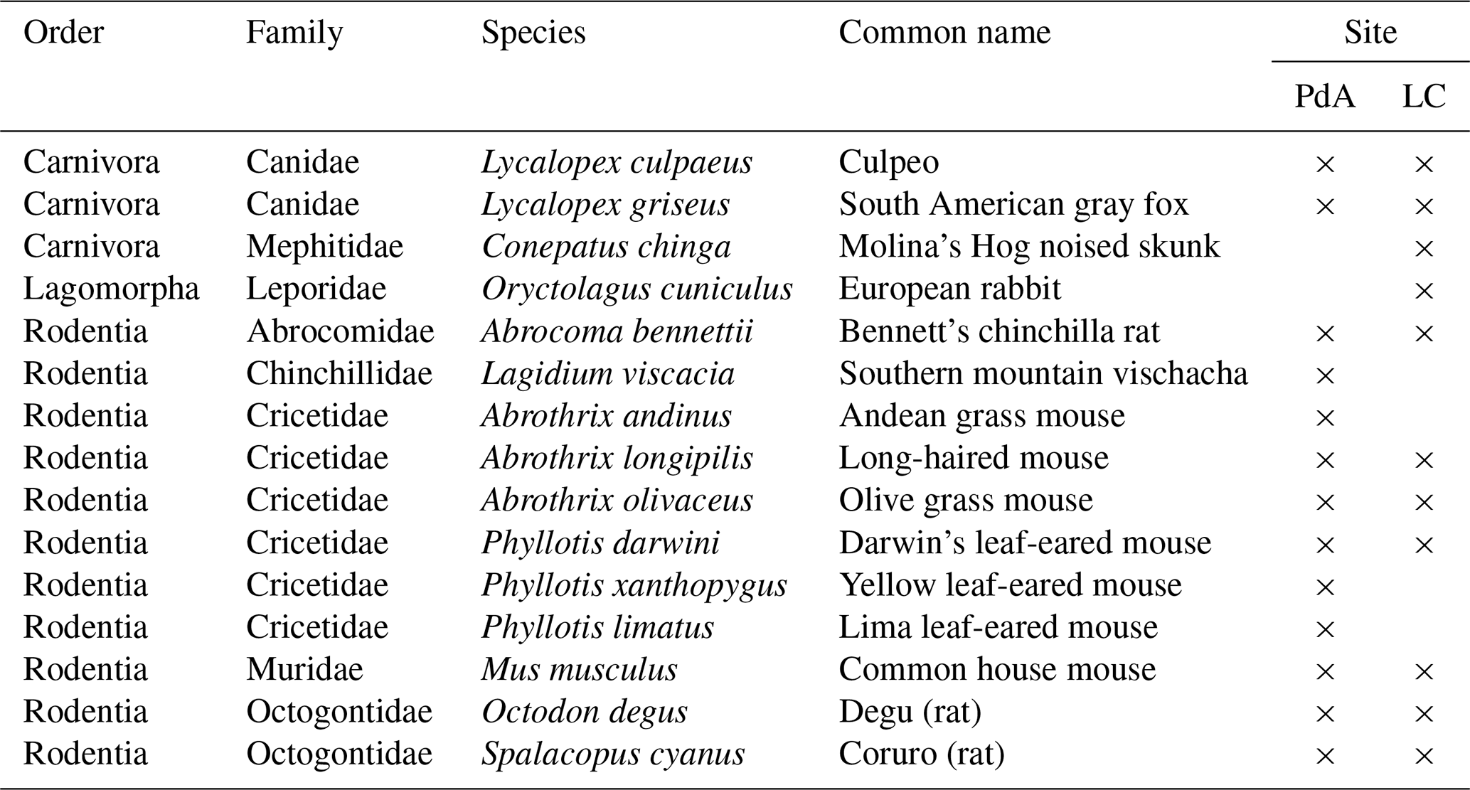
Figure 2 Examples of burrowing vertebrate animals recorded by motion-activated camera traps. (a) Setup of motion-activated camera trap. (b, c) European rabbit (Oryctolagus cunniculus). (d, e) Culpeo (Lycalopex culpaeus). (f) Bennett's chinchilla rat (Abrocoma bennettii). The yellow box highlights the position of the animal in the photo. Photo courtesy of Diana Kraus.

3 Methodology

3.1 Time-of-flight (ToF) principle

A time-of-flight-based camera illuminates an object with a light source, usually in a non-visible spectrum, such as near-infrared, for a precise length of time. ToF cameras rely on the principle of measuring the phase shift, with different options to modulate the light source to be able to measure the phase shift. The here-employed cameras used pulse-based modulation, meaning the light pulse was first emitted by the camera, then reflected from the surface, and finally measured by the camera using two temporary windows. The opening of the first window is synchronized with the pulse emission, i.e., the receiver opens the window with the same Δt as the emitted pulse. Following this, the second window is opened for the same duration Δt, which is synchronized with the closing of the first window. The first temporary window thus measures the incoming reflected light while the light pulse is also still emitting from the camera. The second temporary window measures the incoming reflected light when no pulse is emitting from the camera. The captured photon number (i.e., measured by electrical charge) in both windows can be related according to Eq. (1), and the distance from the camera to the object can then be calculated as follows:

$$\begin{array}{}\text{(1)}& d={\displaystyle \frac{\mathrm{1}}{\mathrm{2}}}\cdot c\cdot t\cdot \left({\displaystyle \frac{g\mathrm{1}}{g\mathrm{1}+g\mathrm{2}}}\right).\end{array}$$

In Eq. (1), d (m) is the distance from the camera to the object, c (m s⁻¹) is the speed of light (299 792 458 m s⁻¹), t (s) is the overall time of the illumination and measurement, g₁ is the ratio of the reflected photons to all photons accumulated in the first window, and g₂ the ratio of the reflected photons to all photons accumulated in the second window (Sarbolandi et al., 2018; Li, 2014).

The sensor in our camera came from Texas Instruments, and the data scan contained information on 320×240 points. The camera field of view (FOV) and the spatial resolution of the scans depended on the height of the camera above the surface and camera orientation. The distance was calculated for every point, and the object was saved in binary format as a collection of 3D points with x, y, and z coordinates. The point clouds taken by the camera were transformed from the binary format to an ASCII format. Each point in the point cloud was assigned to an x, y, and z coordinate. The coordinates were distributed within a three-dimensional Euclidian space, with the point at the camera nadir (the center of the camera sensor) being the point of origin of the 3D Cartesian coordinate system. The x and y coordinates describe the distance to the point of origin (m). The z coordinate describes the distance (m) from the object to the camera. The lowest point of the scanned surface thus has the highest z-coordinate value.

3.2 Data processing

The distortion caused by the hillslope and the camera angle was corrected for each point cloud as follows:

$$\begin{array}{}\text{(2)}& z_{\mathrm{cor}}=z_{\mathrm{uncor}}-\tan (\mathit{\alpha }+\mathit{\beta })\cdot (y_{\mathrm{1}}-y_i).\end{array}$$

In Eq. (2), z_cor is the corrected distance (m) between the camera and surface (m), z_uncor is the uncorrected z coordinate (m), α is the tilt angle of the camera (^∘), and β is the surface inclination (^∘). In addition, y_i (m) is the distance between each point and the point with (i) a y-coordinate = 0 and (ii) the same x coordinate as the point. The most frequent errors were identified and treated as follows. Due to the ambient light reaching the camera sensor, the z-coordinate values of some of the points were incorrect (scattering error). To remove this error, a threshold value was calculated for each point cloud:

$$\begin{array}{}\text{(3)}& \mathrm{\Omega }={\mathrm{mean}}_{\text{z-coordinates}}\pm {\mathrm{SD}}_{\text{z-coordinates}}.\end{array}$$

In Eq. (3), Ω is the threshold value, mean_z-coordinate is the average value, and SD_z-coordinate is the standard deviation of the corrected z coordinates (m). Following this, all points with a z coordinate above and below this value were deleted. Point clouds with more than 50 % of points above the threshold value Ω were also not considered for further processing. A drift error occurred when the z-coordinate values of around one-third of the point clouds decreased by several centimeters from one point cloud to another. Here, the average z coordinate of 10 point clouds before and after the drift were calculated, and the difference was added to z coordinates of the points affected by the drift. The corrected height values were then transformed into a digital surface model (DSM).

3.3 Accuracy of the ToF cameras

The accuracy of the ToF camera was tested under laboratory conditions by recreating similar surface conditions to those in the field (sloping surface, covered by sediment). An artificial mound using sediment extracted from a riverbank in central Germany was used, mimicking a mound created by a burrowing animal. During the test, the camera was installed 100 cm above the surface. The camera FOV was 3 m², and the scan spatial resolution was 6 mm. The surface was scanned twice by the ToF camera. Following this, 100–450 cm³ of sediment was manually extracted from the mound. The volume of the extracted sediment was measured by a measuring cup. After extraction, the surface was again scanned twice by the camera. The experiment was repeated 45 times with varying amounts of extracted sediment. The scans were transformed to point clouds in Voxel Viewer 0.9.10, and the point clouds were corrected according to Eqs. (2) and (3). The z coordinates of the two point clouds before and after the extraction were averaged. The standard deviation of the z coordinate of the two scans was 0.06 cm. Figure A1 shows the spatially distributed standard deviation. The deviation increases from the center towards the corners of the scan. The mound was outlined, and only the points representing the mound were used in the further analysis. The point clouds were then transformed into DSMs, and the differences between the time steps were calculated. A scan was taken of a smooth surface (linoleum floor), and a point cloud was created from the data. Following this, we fitted a plane into the point cloud and calculated the distance between the plane and the camera sensor. The standard variation (0.17 cm) in the distance measurements was saved. Only the differences between the DSMs below this variation were considered in the calculation of the detected sediment extraction. The detected extracted sediment volume was then calculated for each experiment as follows:

$$\begin{array}{}\text{(4)}& {\mathrm{Vol}}_{\mathrm{detected}}={\sum }_p^{\mathrm{1}}\left({\mathrm{DSM}}_{\mathrm{before}}-{\mathrm{DSM}}_{\mathrm{after}}\right)\cdot {\mathrm{res}}^{\mathrm{2}}.\end{array}$$

In Eq. (4), Vol_detected is the volume of the extracted sediment as detected by the camera (cm³), p is the number of pixels, DSM_before (cm) is the DSM calculated from the scan taken before the extraction, DSM_after (cm) is the DSM calculated from the scan taken after the extraction, and res (cm) is the resolution of the scan, which was 0.6 cm. To evaluate the camera's accuracy, the measured volume of the extracted sediment was compared to the volume detected by the camera. The camera's accuracy was estimated between the detected volume and measured volume as follows:

$$\begin{array}{}\text{(5)}& \mathrm{MAE}={\sum }_{\mathrm{1}}^n{\displaystyle \frac{\left({\mathrm{Vol}}_{\mathrm{detected}}-{\mathrm{Vol}}_{\mathrm{measured}}\right)}{\mathrm{area}}}.\end{array}$$

In Eq. (5), MAE (cm³ cm⁻²) is the mean absolute error, n is the number of scans, Vol_measured (cm³) is the volume of the extracted sediment measured by the measuring cup, and the area is the total surface area monitored by the camera (cm²).

3.4 Installation of the cameras in the field

We installed eight custom-tailored ToF-based cameras on four hillslopes in two climate zones located in areas including visible signs of bioturbation activity (burrows) and areas without visible signs of bioturbation (Fig. 3). The cameras were installed at LC on the north-facing upper hillslope (LC-NU), north-facing lower hillslope (LC-NL), south-facing upper hillslope (LC-SU), and the south-facing lower hillslope (LC-SL). At PdA the cameras were installed on the north-facing upper hillslope (PdA-NU), north-facing lower hillslope (PdA-NL), south-facing upper hillslope (PdA-SU), and south-facing lower hillslope (PdA-SL). The custom-tailored cameras were installed during a field campaign in March 2019, the monitoring took place for 7 months, and the data were collected in October 2019. The construction consisted of a 3D ToF-based sensor from Texas Instruments (Li, 2014), a Raspberry Pi single-board computer (SBC), a timer, a 12 V, 12 Ah battery, and three 20 W solar panels for unattended operation (Fig. 2). Solar panels were located at the camera pole and were recharging the battery via a charge controller. The camera was located approximately 1 m above the surface, facing the surface with a tilt angle of 10^∘. The timer was set to close the electric circuit 4 times a day: at 01:00, 05:00, 08:00 and 22:00 GMT−3. At these times, the camera and the computer were turned on for 15 min. The camera turned on and took five scans delayed 1 s from each other and sent them to the SBC. Each camera had its own WiFi, and the data could be read from the SBC via Secure Shell (SSH). The cameras collected the data for the time period of 7 months.

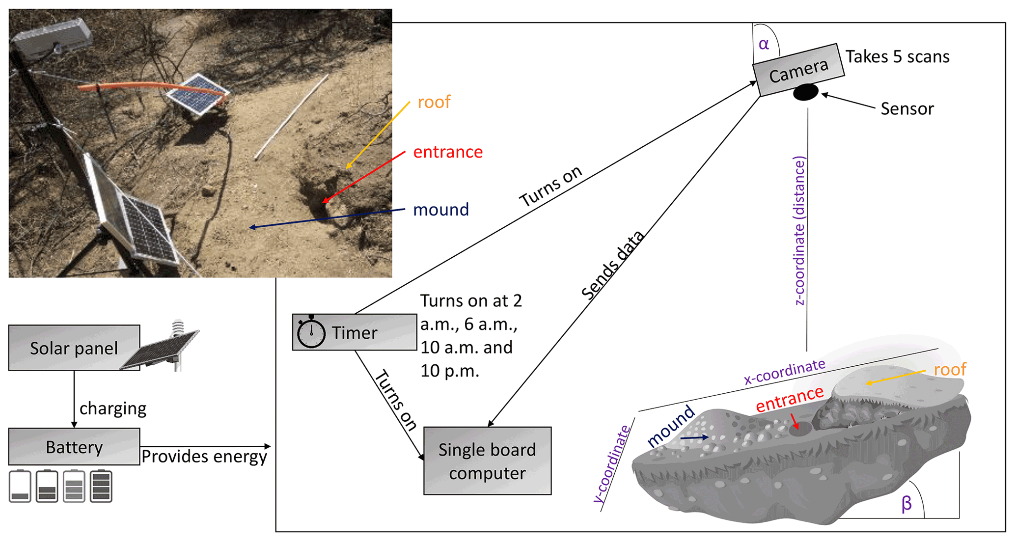
Figure 3 Scheme and photo example of a time-of-flight-based camera installation in the field. The photo example is from north-facing upper hillslope at La Campana. Black boxes describe single installation parts. Purple descriptions are the variables needed for the correction of the scans. Roof, entrance, and mound describe parts of the burrow. The x, y, and z coordinates are 3D coordinates identifying the position of each point in space, where the x coordinate is the length, the y coordinate is the width, and the z coordinate is the distance between the camera sensor and the surface. α is the inclination of the camera, and β is the surface inclination.

3.5 Delineation of burrows and burrow-embedded areas

The surface area scanned by the cameras was divided by a delineation scheme into burrows (B) and burrow-embedded areas (EM). The burrows included three sub-areas: (i) mound (M), (ii) entrance (E), and (iii) burrow roof (R). “Mound” describes the sediment excavated by the animal while digging the burrow. “Entrance” describes the entry to the animal burrow up to the depth possible to obtain via the camera. “Burrow roof” describes the part of the sediment above and uphill the burrow entrance (Bancroft et al., 2004). During the burrow's creation, sediment was not only excavated but also pushed aside and uphill from the entrance, which created the burrow roof. We assume that this elevated microtopographical feature then forms an obstacle for sediment transported from uphill, which leads to its accumulation in this area. The remaining surface within the camera's FOV was the burrow-embedded area. Please note that this area may still be affected by the burrowing activity of the animal and is not completely unaffected by the animal.

For the delineation, we used the DSM calculated from the point cloud and a slope layer calculated from the DSM (Horn, 1981). The DSM had a size of 4 m² and a resolution of 0.6 cm. Entrance was assigned to an area determined by a search algorithm starting at the lowest point of the DSM (the pixel with the highest z-coordinate value). We increased the circular buffer around the starting point by one pixel until the average depth of the new buffer points was not higher than the height of the camera above the surface or until the slope of at least 50 % of the new buffer points was not 0. Following this, we masked all pixels within the buffer with a depth lower than the average depth of the points within the buffer, which had a slope that was 0. The remaining pixels belonged to the entrance area. Then, the surface scan was divided into an uphill and downhill part with regards to the entrance position. Both the uphill and the downhill parts were subdivided into 16 squares, so that each of the four quadrants within the 2D grid (x- and y-axis) contained four squares. The squares had size of 0.5 m².

To delineate the mound in the downhill part, we first identified the highest points (pixel with the lowest z-coordinate value) within all 16 squares. We then calculated the distance of these maxima to the entrance, and the pixel located nearest to the entrance was identified as the highest point of the mound (i.e., seed point). Consecutively, we increased the circular buffer around the seed point by one pixel until the average depth of the new buffer points was not lower than the height of the camera above the surface, or until the slope of at least 50 % of the new buffer points was not 0. Then, we masked all pixels within the buffer with a depth higher than the average depth of the points within the buffer, which had a slope that was 0. The remaining pixels were classified as mound area. To delineate burrow roof, we used the same approach as for the delineation of mound and applied it on the uphill part of the surface scan. We used the digital elevation model (DEM) and slope layers for the delineation for several reasons. The distance from the surface to the camera was the most important parameter to derive (i) the deepest point of the entrance and (ii) the highest point of the mound or burrow roof, as this was (mostly) the closest point to the camera. After the angle correction of the z-coordinate according to Sect. 3.2., the surface inclination of the areas without burrow was 0^∘, while the angle between the border of the burrow entrance or mound and the burrow-embedded surface was above 0^∘. Because neither the entrance nor the mound have a perfect circular form, we would largely overestimate or underestimate the entrance or mound size. Overestimations would occur if we did not stop the search algorithm until the angle between all new points of the buffer to the rest of the buffer was 0^∘. Underestimations would occur if we stopped the algorithm when the angle of one point of the buffer to the nearest point of the buffer was 0^∘. The value of 50 % thus minimized the error. All pixels that were not classified during the entire delineation process were treated as burrow-embedded areas.

The position and the boundaries of entrance, mound, and burrow roof were validated visually (Figs. 4 and A2).

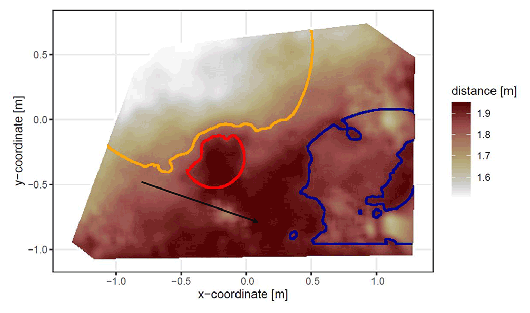
Figure 4 Corrected digital surface model of the camera on the north-facing upper hillslope at La Campana with delineated areas. The point of origin of the coordinate system is at the camera nadir. Distance refers to the distance between surface and camera. The red line delineates the burrow entrance, the blue line delineates the mound, and the orange line delineates the burrow roof. The area that was outside of any delineated area was classified as burrow-embedded area. The arrow indicates a downhill direction of the hillslope.

At LC, the burrows always consisted of an entrance, mound, and burrow roof. At PdA, there was no burrow roof on the upper hillslopes. Burrows without a burrow roof were located on shallower parts of the hillslopes (up to an inclination of 5^∘), and the angle of the burrow entrance to the ground was ∼ 90^∘. Burrows with a burrow roof were located on steeper parts of the hillslopes (with an inclination above 5^∘), and the angle of the burrow entrance to the ground was ∼ 45^∘.

3.6 Calculation of animal-caused and rainfall-caused sediment redistribution

We compared the DSMs of each scan pairwise with the previously saved scan and identified three types of sediment redistribution that occurred in the time period between these images. The three types of redistribution were as follows: (a) animal-caused redistribution; (b) rainfall-caused redistribution; (c) both animal- and rainfall-caused redistribution.

The animal-caused sediment redistribution occurred when the animal actively reworked sediment within its burrow. The following five prerequisites had to be met when the sediment redistribution was caused solely by the animal: (i) as the animal excavates sediment from the entrance, the depth of the entrance must increase in the second scan, (ii) as the excavated sediment accumulates on the mound, the height of the mound must increase in the second scan, (iii) as the burrowing might lead to an expansion or a collapse of the burrow roof, an increase or decrease of the burrow roof must occur between the scans, (iv) as the animal only digs within its burrow, no changes must occur between the two scans within the burrow-embedded area by the animal, and (v) no rainfall can have occurred during this period.

The rainfall-caused sediment redistribution was calculated as follows: from the data from the climate stations (Übernickel et al., 2021a), we calculated the daily precipitation in millimeters. The sediment redistribution recorded immediately and within five scans before and after a rainfall event is defined to be the result of the rainfall event. This was necessary as the climate stations are located up to a 15 km distance from the cameras (Fig. 1). To attribute a sediment redistribution to a rainfall event, the following three preconditions had to be met: (i) a rainfall event occurred; (ii) sediment is eroded from burrow roof, mound, and the embedding area; and (iii) sediment is accumulated within the burrow entrance.

To attribute sediment redistribution to a combination of animal activity and rainfall, the following four preconditions had to be met: (i) a rainfall event occurred, (ii) sediment is eroded from embedding area, (iii) the height of burrow roof and mound decreased or increased, and (iv) the depth of burrow entrance increased.

The animal-caused sediment redistribution was calculated as the sediment volume excavated from the entrance. Animal excavation always increased the depth of the burrow entrance. The rainfall-caused sediment redistribution was calculated as the sediment volume that eroded from the burrow roof and mound. During a rainfall event, sediment eroding from burrow roof might accumulate within burrow entrances. In this case, the depth of the burrow entrance decreased. No sediment could erode from the entrance during a rainfall event. Decreased depth of a burrow entrance always points to sediment redistribution caused by rainfall, while increased depth of burrow entrance always means redistribution by animals. Rainfall-caused redistribution always occurred before animal-caused redistribution, as without erosion caused by rainfall, the animals did not need to reconstruct their burrows.

3.7 Calculation of daily sediment mass balance budget

The volume of the redistributed sediment was calculated daily and was then cumulated from the first day of monitoring. For the calculation of the daily sediment redistribution, the change in the surface level detected by the camera was calculated first. For each day, the scans from the day before and after the respective day were averaged and subtracted. The average standard deviation of the z-coordinate of these scans was 0.06 cm. As described in Sect. 2.2., all values with a difference below and above the threshold value of 0.2 cm were set to 0. The redistributed sediment volume was then calculated from the surface change for each pixel as follows:

$$\begin{array}{}\text{(6)}& {\mathrm{Vol}}_{\mathrm{redistributed}}=(S_{\mathrm{b}}-S_{\mathrm{a}})\cdot {\mathrm{res}}^{\mathrm{2}}.\end{array}$$

In Eq. (6), Vol_{redistributed} (cm³ pixel⁻¹) is the volume of the calculated redistributed sediment, S_b (cm) the scan before the rainfall event, S_a (cm) is the scan after the rainfall event, and res is the spatial resolution (cm). Using the daily volume of the redistributed sediment per pixel, we calculated the daily mass balance budget by summing the volume of sediment eroding or accumulating within each delineated area.

3.8 Calculation of the overall volume of redistributed sediment after the period of 7 months

From the camera data, we calculated the average cumulative volume of redistributed sediment for the period of 7 months within burrows (Vol_burrows (cm³ cm⁻² yr⁻¹)) and burrow-embedded areas (Vol_embedding (cm³ cm⁻² yr⁻¹)) and the average sediment volume redistributed (excavated) by the animal (Vol_exc (cm³ cm⁻² yr⁻¹)) separately for each site. We estimated the volume of sediment that was redistributed during rainfall events due to the presence of the burrow (Vol_add (cm³ cm⁻² yr⁻¹)). Vol_add was calculated as the difference in the redistributed sediment volume between burrows and burrow-embedded areas according to Eq. (7).

$$\begin{array}{}\text{(7)}& {\mathrm{Vol}}_{\mathrm{add}}=\left({\mathrm{Vol}}_{\mathrm{affected}}-{\mathrm{Vol}}_{\mathrm{unaffected}}\right)\cdot \mathrm{1.71}\end{array}$$

Additionally, we calculated the average volume of the redistributed sediment per burrow (Vol_per burrow, cm³ burrow⁻¹ yr⁻¹).

$$\begin{array}{}\text{(8)}& {\mathrm{Vol}}_{\mathrm{per}\mathrm{burrow}}=\left({\mathrm{Area}}_{\mathrm{burrow}}\cdot \mathrm{Vol}\right)\cdot \mathrm{1.71}\end{array}$$

In Eq. (8), Area_burrow (cm²) is the average size of the burrows that are monitored by the cameras and Vol is Vol_burrow (cm³ cm⁻² yr⁻¹), Vol_exc (cm³ cm⁻² yr⁻¹), or Vol_add (cm³ cm⁻² yr⁻¹).

We then upscaled the Vol_burrow (cm³ cm⁻² yr⁻¹), Vol_exc (cm³ cm⁻² yr⁻¹), and Vol_add (cm³ cm⁻² yr⁻¹) to the hillslope using the following approach. Hillslope-wide upscaling of the results generated in this study was performed by using a previous estimation of vertebrate burrow density (Grigusova et al., 2021). In this study, the density of burrows was measured in situ within 80 total 100 m² plots and then upscaled to the same hillslopes on which the cameras were located by applying machine-learning methods, using the uncrewed aerial vehicle (UAV) data as predictors. For upscaling, we applied a random forest model with recursive feature elimination. The model was validated by a repeated leave-one-out cross validation. The density of vertebrate burrows was between 6 and 12 100 m² at LC and between 0 and 12 100 m⁻² at PdA. Using the hillslope-wide predicted vertebrate burrow densities (Dens_burrow (number of burrows 100 m⁻²)) from Grigusova et al. (2021), we estimated the volume of redistributed sediment for each pixel of the raster layers (Vol_per pixel (cm³ m⁻² yr⁻¹)) according to Eq. (9):

$$\begin{array}{}\text{(9)}& {\mathrm{Vol}}_{\mathrm{per}\mathrm{pixel}}={\mathrm{Vol}}_{\mathrm{per}\mathrm{burrow}}\cdot {\mathrm{Dens}}_{\mathrm{burrow}}\cdot \mathrm{1.71}.\end{array}$$

The average hillslope-wide volume of redistributed sediment (Vol_{hillslope-wide} (m³ ha⁻¹ yr⁻¹)) was then estimated as follows:

$$\begin{array}{}\text{(10)}& {\mathrm{Vol}}_{\text{hillslope-wide}}={\sum }_{\mathrm{1}}^m{\mathrm{Vol}}_{\mathrm{per}\mathrm{pixel}}\cdot \mathrm{0.001}\cdot \mathrm{1.71}.\end{array}$$

In Eq. (10), m is the number of pixels.

4 Results

4.1 Camera accuracy and data availability

The accuracy between the measured extracted sediment volume and sediment volume calculated from the camera scans was very high (MAE = 0.023 cm³ cm⁻²; R²= 0.77; SD = 0.02 cm³ cm⁻², Fig. A3). The accuracy between the calculated and measured extracted sediment was higher when the two scans taken before and after the extraction of the sediment were averaged and the sediment volume was estimated using these averaged scans. When calculating the redistributed sediment from solely one scan before and after extraction, the accuracy slightly decreased (MAE = 0.081 cm³ cm⁻², R²= 0.64). The cameras tended to overestimate the volume of redistributed sediment. Six out of eight custom-tailored cameras collected data over the 7-month period (Table A2). One camera collected data for a period of 3 months and one camera stopped working a few days after installation. The quantity of usable point clouds taken at 01:00, 05:00, and 22:00 GMT−3. was higher than of point clouds taken at 08:00. Approximately 20 % of points were removed from the point clouds before final analysis due to the high scattering at the point cloud corners. After data filtering (see Sect. 3.2.), 1326 scans were usable, and at least one usable scan was available for 86 % of the days. The usable scans were distributed continuously within the monitoring period.

4.2 Mass balance of redistributed sediment

The cameras detected (i) sediment redistribution directly following rainfall events and (ii) due to the burrowing activity in times without rainfall (Figs.  5, A4 and A5). In all cases, burrows (entrance, burrow roof, and mound) exhibited higher sediment redistribution rates than burrow-embedded areas. In addition, the volume of redistributed sediment by animal activity was higher after a rainfall event occurred.

In the following, the dynamics are exemplary explained for four cameras. Animal burrowing activity was detected seven times by the camera LC NU (Figs. 5a, A4, A5) during the monitoring period by an increase in sediment volume in the area delineated as mound. Simultaneously, the burrow entrance showed signs of modification and sediment accumulation, but these changes were less clear. Overall, the volume of the excavated soil varied. From April until June, up to 0.5 cm³ cm⁻² of sediment was excavated by the animal and accumulated on the mound. From June until September, animal burrowing activity was detected at four time slots (5 June, 9 June, 1 July, and 18 August 2019) and sediment volume of up to 2 cm³ cm⁻² accumulated each time on the mound, on the burrow roof, and within the entrance. During the rainfall events of up to 20 mm d⁻¹ on 16 June 2019, 27 mm d⁻¹ on 29 June 2019, and 7 mm d⁻¹ on 13 July 2019, sediment volume of up to 4 cm³ cm⁻² eroded, especially from the burrow roof and the mound, while a sediment volume of up to 1 cm³ cm⁻² accumulated within the entrance during each rainfall event. Camera LC-SL (Figs. A4, A5) showed burrowing activities eight times, and sediment volumes of up to 3 cm³ cm⁻² accumulated within the entrance and burrow roof. The camera detected sediment erosion of up to 2 cm³ cm⁻² after a rainfall event of 27 mm d⁻¹ on 27 July 2019. On the south-facing upper hillslope, the camera detected animal burrowing activity six times, with a sediment accumulation of up to 3 cm³ cm⁻² (Figs. A2 and A3).

In contrast, camera PdA-NU pointed to animal burrowing activity up to 15 times, where up to 1 cm³ cm⁻² of sediment volume was redistributed from the entrance to the mound (Figs. 5b, A4, A5). At the end of June on 27 June 2019, a rainfall event of 1.5 mm d⁻¹ occurred and up to 2 cm³ cm⁻² of sediment eroded from the burrow roof and accumulated within the burrow entrance. We observed increased sediment redistribution by the animal after the rainfall events. Camera PdA-SL similarly revealed animal burrowing activity up to 15 times (Figs. A4, A5). The burrowing had a strong effect on the sediment redistribution. The rainfall event of 1.5 mm d⁻¹ on 27 June 2019 did not cause any detectable surface change.

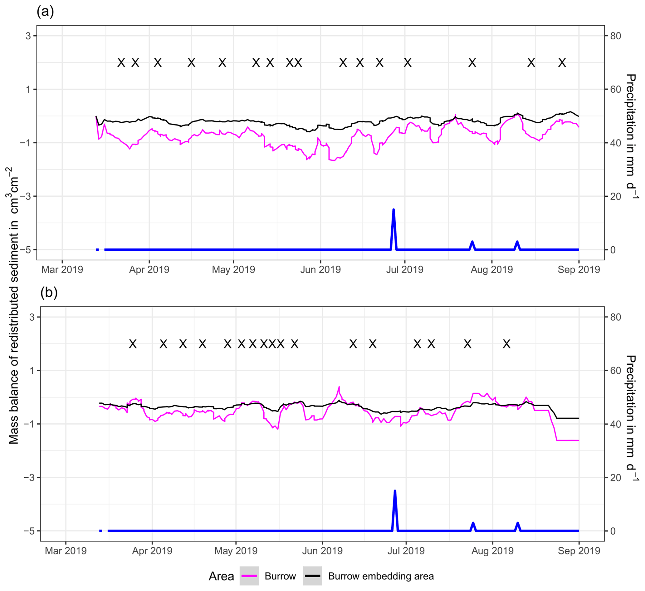
Figure 5 Examples of the mass balance of redistributed sediment for burrows and burrow-embedded areas. (a) The record of the camera on the north-facing upper hillslope at La Campana showed that larger rainfall events cause a negative sediment balance (sediment loss), followed by a phase of positive sediment mass balance after approximately 3 d due to sediment excavation; (b) The record of the camera on the north-facing upper hillslope in Pan de Azúcar showed a similar pattern to the camera on the north-facing upper hillslope, but the phase of positive mass balance was delayed in comparison. The blue line is the daily precipitation (in mm d⁻¹), and “X” marks the days at which animal burrowing activity was detected. Positive values indicate sediment accumulation. Negative values indicate sediment erosion. Mass balances for all cameras are displayed in Figs. A2 and A3.

The analysis of cumulative volume of the redistributed sediment caused by burrowing animal activity and rainfall over the monitored period of 7 months for all eight cameras showed a heterogeneous pattern.

At LC, the cumulative volume of the sediment excavated by the animal within the burrow roof and mound increased continuously (Figs. 6, A7). Specifically, a cumulative volume of 6.5 cm³ cm⁻² was excavated on average by the animal between the rainfall events from June until August. We calculated that 8.53 cm³ cm⁻² cumulatively eroded from the burrow roof and mound on average, whereas 2.44 cm³ cm⁻² sediment volume accumulated within the entrance (Figs. 6, A7). These results indicate that 28 % of sediment eroding from the burrow roof accumulated within the entrance, while over 62 % of sediment eroded downhill. Averaged over all camera scans, 338 % more sediment was redistributed by rain within burrow compared to the burrow-embedded area (Fig. 7).

At PdA, cameras continuously detected animal burrowing activity and excavation of the sediment (Fig. A7). The volume of the detected excavated sediment increased steadily within all cameras. The cumulative sediment accumulation surpasses the sediment eroded due to the rainfall. The volume of the sediment eroded within the burrows was 40 % higher than within the burrow-embedded areas. The results show that approximately 50 % of the eroded sediment accumulated within the entrance (Fig. 7).

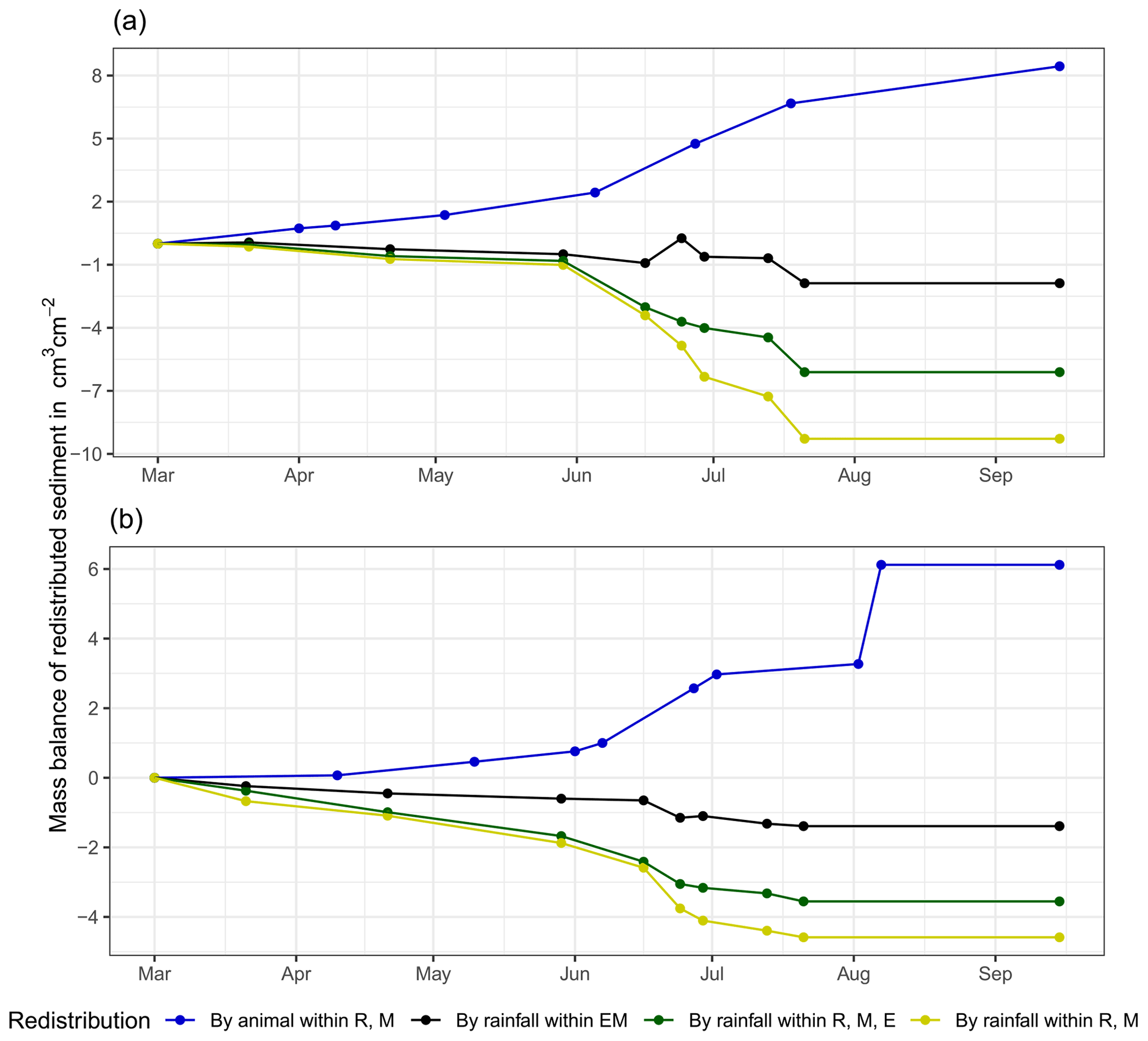
Figure 6 Examples of the cumulative volume of redistributed sediment within burrows and burrow-embedded areas caused by animal burrowing activity or rainfall in the Mediterranean climate zone of La Campana for the (a) north-facing upper hillslope and (b) south-facing lower hillslope. Positive values indicate sediment accumulation. Negative values indicate sediment erosion. E is the burrow entrance, M is the mound, R is the burrow roof, and EM is the burrow-embedded area. Cumulative volumes for all cameras are given in Fig. A7.

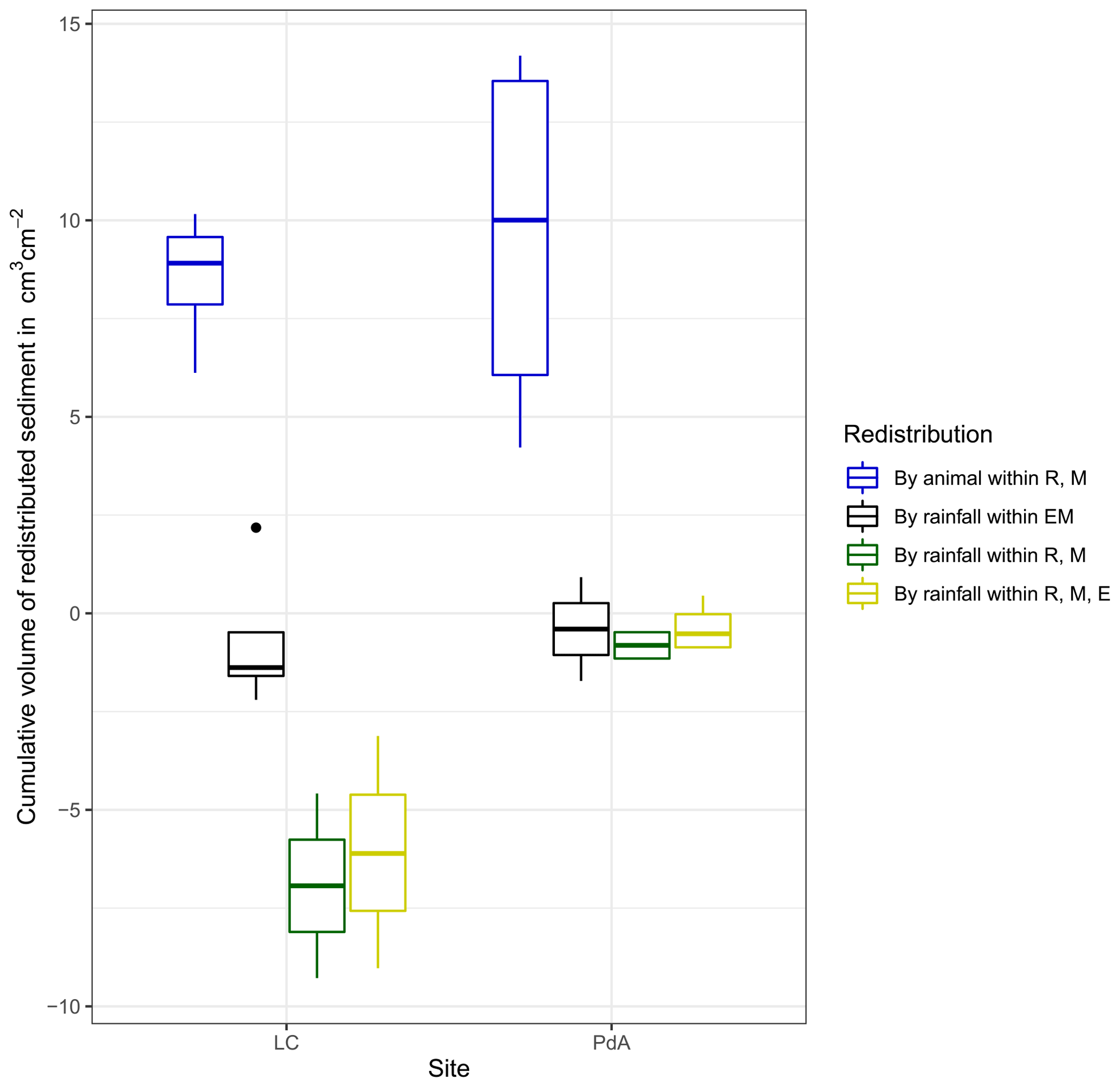
Figure 7 Cumulative volume of the redistributed sediment for the time period of 7 months for all cameras. Positive values indicate sediment accumulation. Negative values indicate sediment erosion. Whiskers indicate the median of sediment redistribution. E is the burrow entrance, M is the mound, R is the burrow roof, EM is the burrow-embedded area, LC stands for National Park La Campana (in the Mediterranean climate zone), and PdA stands for National Park Pan de Azúcar (in the arid climate zone).

4.3 Volume of redistributed sediment

The average size of the burrows was 84.3 cm² (SD = 32.5 cm²) at LC and 91.3 cm² at PdA (SD = 8.5 cm²). The animals burrowed on average 1.2 times a month at LC and 2.3 times a month at PdA. The volume of the excavated sediment was 102.2 cm⁻³ per month at LC and 124.8 cm³ per month at PdA. Each time the animals burrowed, they excavated 42 cm³ sediment volume at LC and 14.3 cm³ sediment volume at PdA. The burrowing intensity increased in winter after the rainfall occurrences at LC and stayed constant during the whole monitoring period at PdA. The burrows deteriorate after rainfall events with a rate of 73.0 cm³ per month or 63.9 cm³ per event at LC and 10.5 cm⁻³ per month or 24.5 cm³ per event.

The overall volume of the sediment excavated by the animals and redistributed during rainfall events varied between the sites (Table 1). The volume of the sediment redistributed by the animal was lower at LC than at PdA. However, on the hillslope scale, a higher total area-wide volume of excavation was calculated for LC compared to PdA due to the higher burrow density at LC. The volume of the sediment redistributed within burrows during rainfall events was higher at LC than at PdA. The volume of additionally redistributed sediment due to the presence of burrows was higher at LC than at PdA (Table 2, Fig. 8).

Table 2 Summary of the volume of redistributed sediment according to area and disturbance type. Vol_exc describes volume of the sediment excavated by the animals. Vol_burrow describes volume of the sediment redistributed during rainfall events within burrows. Vol_add describes the difference in redistributed sediment volume within burrows and burrow embedding areas during rainfall. Positive values indicate sediment accumulation, while negative values indicate sediment erosion.

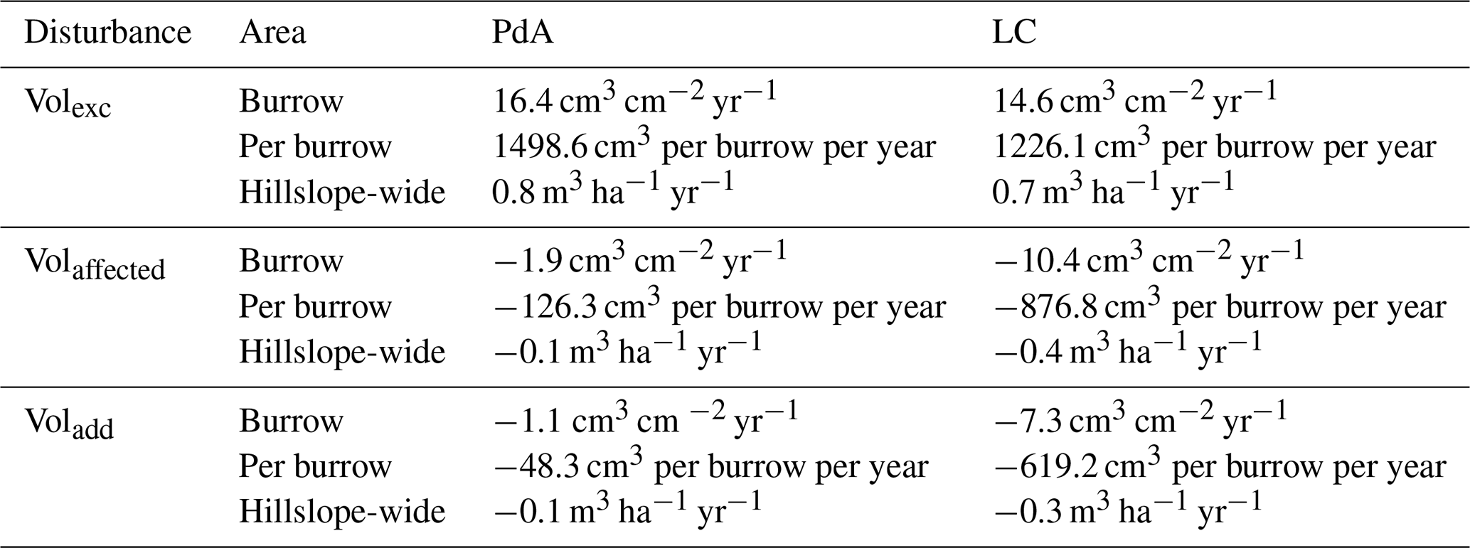
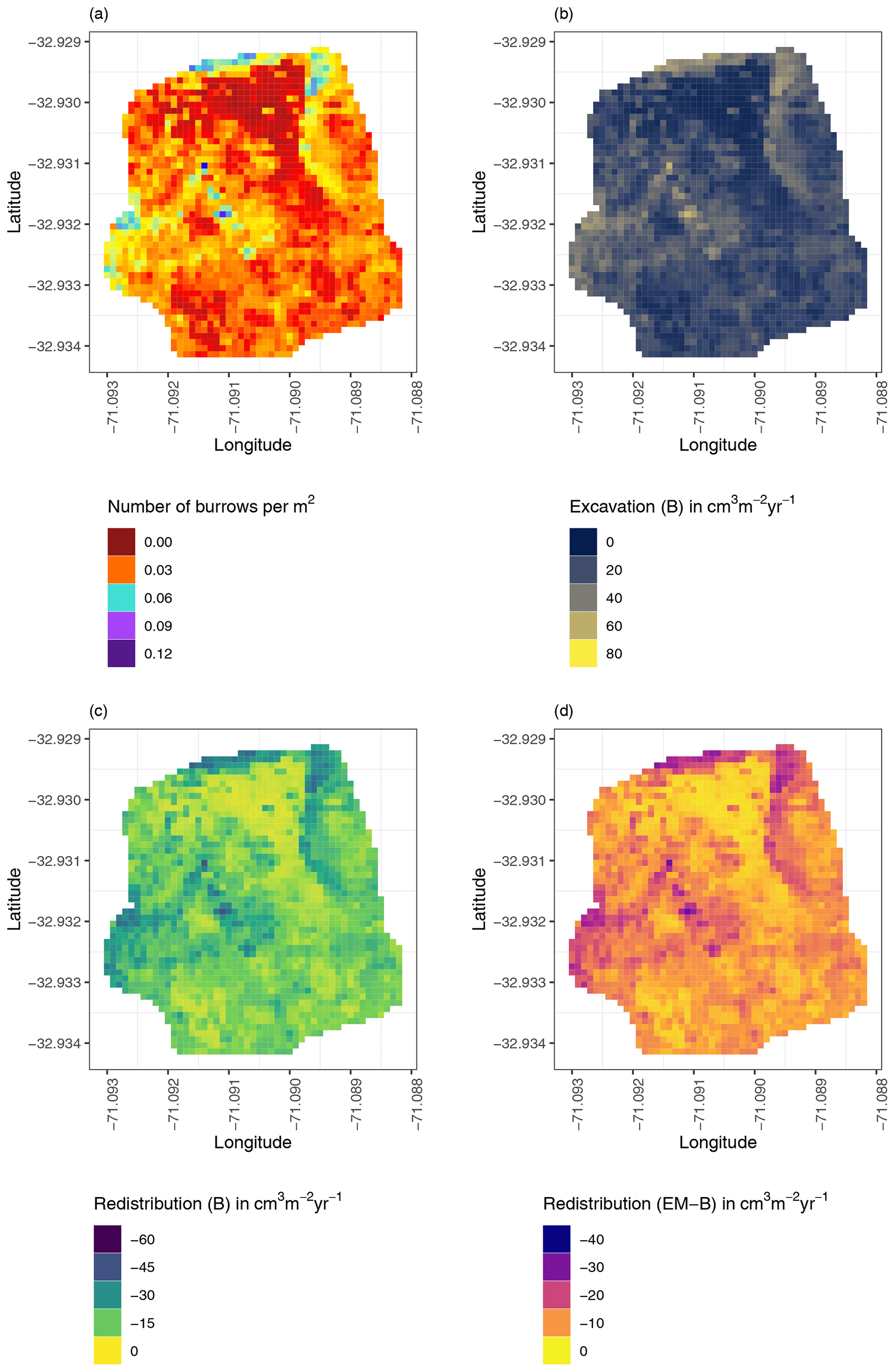
Figure 8 Example of the hillslope-wide volume of redistributed sediment on the south-facing hillslope at La Campana: (a) density of burrows as estimated by Grigusova et al. (2021), (b) volume of the sediment excavated by the animals, (c) volume of the sediment redistributed during rainfall events within burrows, and (d) volume of additionally redistributed sediment during rainfall events due to the presence of the burrows. The values were calculated per burrow, as stated in Sect. 3.7., by subtracting the sediment volume redistributed within burrows from the sediment volume redistributed within the burrow-embedded area and then upscaled. The letters in brackets indicate if the upscaling was conducted using data from burrows or burrow-embedded areas. “B” stands for burrow. By “EM-B”, the redistribution calculated within burrow-embedded areas was subtracted from the redistribution calculated within burrows to obtain the additional volume of redistributed sediment due to the burrows' presence. Positive values indicate sediment accumulation. Negative values indicate sediment erosion.

5 Discussion

Our results showed that the custom-made ToF device is a suitable tool for high-resolution, automated monitoring of surface changes that is also applicable in remote areas. The continuous observation of sediment redistribution over a longer time period provided new insights into the relative importance of burrowing animals for hillslope sediment flux. Our research revealed that the presence of vertebrate burrows increases hillslope sediment redistribution rates much more than previously assumed (increase of up to 208 %). We showed that the quantity of animal-related sediment redistribution, however, varied with rainfall occurrence, with an increase in sediment redistribution between 40 % in the arid climate zone research area and 338 % percent in the Mediterranean climate zone research area.

5.1 Suitability of the ToF cameras for surface monitoring

The newly introduced monitoring technique ToF enables an automatic monitoring of surface changes on a microtopographic scale and is less costly and invasive than other techniques. The measurement continuity of the device also allows for the analysis of ongoing biogeomorphological processes at high temporal and spatial resolution.

With regard to the costs, measurement frequency, and sampling autonomy, the custom-made ToF device constitutes an improvement to earlier studies that used laser scanning technology to monitor microtopographic changes (Table A5). This is because previous studies applied expensive laser scanning for the estimation of sediment redistribution, and due to the costs of the instrument it was not left in the field for continuous measurements. Hence, research sites had to be revisited for each measurement (Nasermoaddeli and Pasche, 2008; Eltner et al., 2016b, a; Hänsel et al., 2016). The estimated costs in studies using time-lapse photogrammetry were similar to our study (up to USD 5000) (James and Robson, 2014; Galland et al., 2016; Mallalieu et al., 2017; Eltner et al., 2017; Kromer et al., 2019; Blanch et al., 2021). However, time-lapse monitoring needs several devices set up in different viewing angles, which increases installation efforts and disturbance significantly.

In terms of data quality, our ToF device is more precise or comparable to those employed in earlier studies using ToF. The accuracy of the camera (R²= 0.77) was in the range of previous studies (R²= 0.26–0.83 (Eitel et al., 2011, Table A5). The horizontal point spacing of our cameras was 0.32 cm, and the maximum number of points per square centimeter was 8.5. These values are similar to previous studies in which the used devices had a horizontal point spacing in the range of 0.25–0.57 cm (Kaiser et al., 2014; Nasermoaddeli and Pasche, 2008) (Table A5), and the maximum number of points per square centimeter in a range of 1 to 25 points per square centimeter (Eitel et al., 2011; Longoni et al., 2016) (Table A5).

Our cameras tended to slightly overestimate or underestimate the volume of redistributed sediment. This error occurs when the pulse reflects from several vertical objects such as walls or, in our case, branches or stones and then enters the camera sensor. This phenomenon was also observed in previous studies applying laser scanners and is inevitable if the goal is to study surface changes under natural field conditions (Kukko and Hyyppä, 2009; Ashcroft et al., 2014). During operation of the cameras, we learned that our newly developed instruments are particularly capable of delivering usable scans at night. This is likely due to the strong scattered sunlight reaching the camera sensor during the day and blurring the data (Li, 2014). Thus, in future studies, we recommend focusing on nocturnal operation to prevent light contamination.

5.2 The role of climate variability and burrowing cycles

We have found that rainfall plays a key role in triggering burrowing activity, which means that wet seasons experience higher sediment redistribution rates than dry seasons. In the year of investigation (2019), the dry season lasted from January until April and from September until December (8 months), while the wet season lasted from May until August (4 months). The monitoring period lasted from March until October, which covered 3 dry and 4 wet months (7 months in total). A yearly rate of sediment redistribution can be calculated by simply averaging the redistribution rate of the 7 monitored months and multiplying this result by 12 months, which results in an average redistribution rate of 0.4 m² ha⁻¹ yr⁻¹ for LC and 0.1 m² ha⁻¹ yr⁻¹ for PdA. However, because burrowing activity and rain-driven sediment redistribution is mainly determined by rainfall, this method might have led to an overestimation of the annual redistribution rate based on averaging because the unmonitored part of the year 2019 was predominantly dry (Übernickel et al., 2021a). This can be accounted for by adding 5 times the dry month redistribution rate to the monitored 7 months, which leads to a lower annual redistribution rates for LC of 0.3 m² ha⁻¹ yr⁻¹ and for PdA of 0.1 m² ha⁻¹ yr⁻¹. Our values might thus overestimate sediment redistribution for the year 2019. This difference between both values (0.1 m² ha⁻¹ yr⁻¹ for LC and under 0.1 m² ha⁻¹ yr⁻¹ for PdA) can be interpreted as the uncertainty range for the year of observation.

However, decadal rainfall variability indicates that the year of monitoring (2019) was among the drier years of the last 30 years (Yáñez et al., 2001; Valdés-Pineda et al., 2016; Garreaud et al., 2002; Wilcox et al., 2016). The amount of precipitation since 1980 ranges from 200 to 800 mm yr⁻¹ (https://climatologia.meteochile.gob.cl/application/requerimiento/producto/RE3005, last access: 19 September 2022), while the amount of precipitation in 2019 was just above 100 mm. This means that our results might underestimate sediment redistribution on a longer timescale by 2–7 times.

Furthermore, the phenology of the burrowing animals is an additional source of uncertainty when calculating annual rates. The most common burrowing animal families in the area are active for 3 months of the year. The months in which they are active are between April and September. None of the most common burrowing animal families were reported to be active from November until February. (Eccard and Herde, 2013; Jimenez et al., 1992; Katzman et al., 2018; Malizia, 1998; Monteverde and Piudo, 2011). This is also in line with our observations because burrowing intensity increased from March until May, reached its peak between May and June, and declined until September (Fig. 6). By extrapolating from 7 months to a 1-year period, our estimated excavation was 0.7 m² ha⁻¹ yr⁻¹ at LC and 0.8 m² ha⁻¹ yr⁻¹ at PdA. By the dry season to the 7 months of observation, the estimated excavation would be 0.6 m² ha⁻¹ yr⁻¹ at LC and 0.6 m² ha⁻¹ yr⁻¹ at PdA. Our values might thus overestimate the sediment excavation, and the excavation uncertainty range is 0.1 m² ha⁻¹ yr⁻¹ for LC and 0.2 m² ha⁻¹ yr⁻¹ for PdA.

5.3 Sediment redistribution

Our research reveals that the presence of vertebrate burrows generally increases hillslope sediment redistribution. We show, however, that the ratio between the sediment redistribution caused by rainfall within burrow and burrow-embedded areas varies between climate zones. Sediment redistribution within burrow areas was 40 % higher at the arid research site, and at the Mediterranean research site it was 338 % higher when compared to burrow-embedded areas (Table A6).

By monitoring microtopographical changes in a high spatiotemporal resolution, we found that the occurrence of larger rainfall events played a 2-fold accelerating role in influencing sediment redistribution (Fig. 9). Firstly, rainfall-runoff-eroded burrow material caused increased sediment loss. This was followed by animal burrowing activity after the rainfall. This means that rainfall triggered animal burrowing activity that was very likely related to the lower burrowing resistance of the soil due to the increased soil moisture (Rutin, 1996; Romañach et al., 2005; Herbst and Bennett, 2006). This double feedback led to frequently occurring but small redistribution rates. However, the mechanism cumulatively increased downhill sediment fluxes. Previous studies most likely missed these low-magnitude but frequent surface processes due to their lower monitoring duration and frequency or artificial laboratory conditions, and thus they did not quantify the full volume of redistributed sediment associated with burrowing activity. To quantify all occurred sediment redistribution processes, a continuous surface monitoring framework (like the one presented here) is needed.

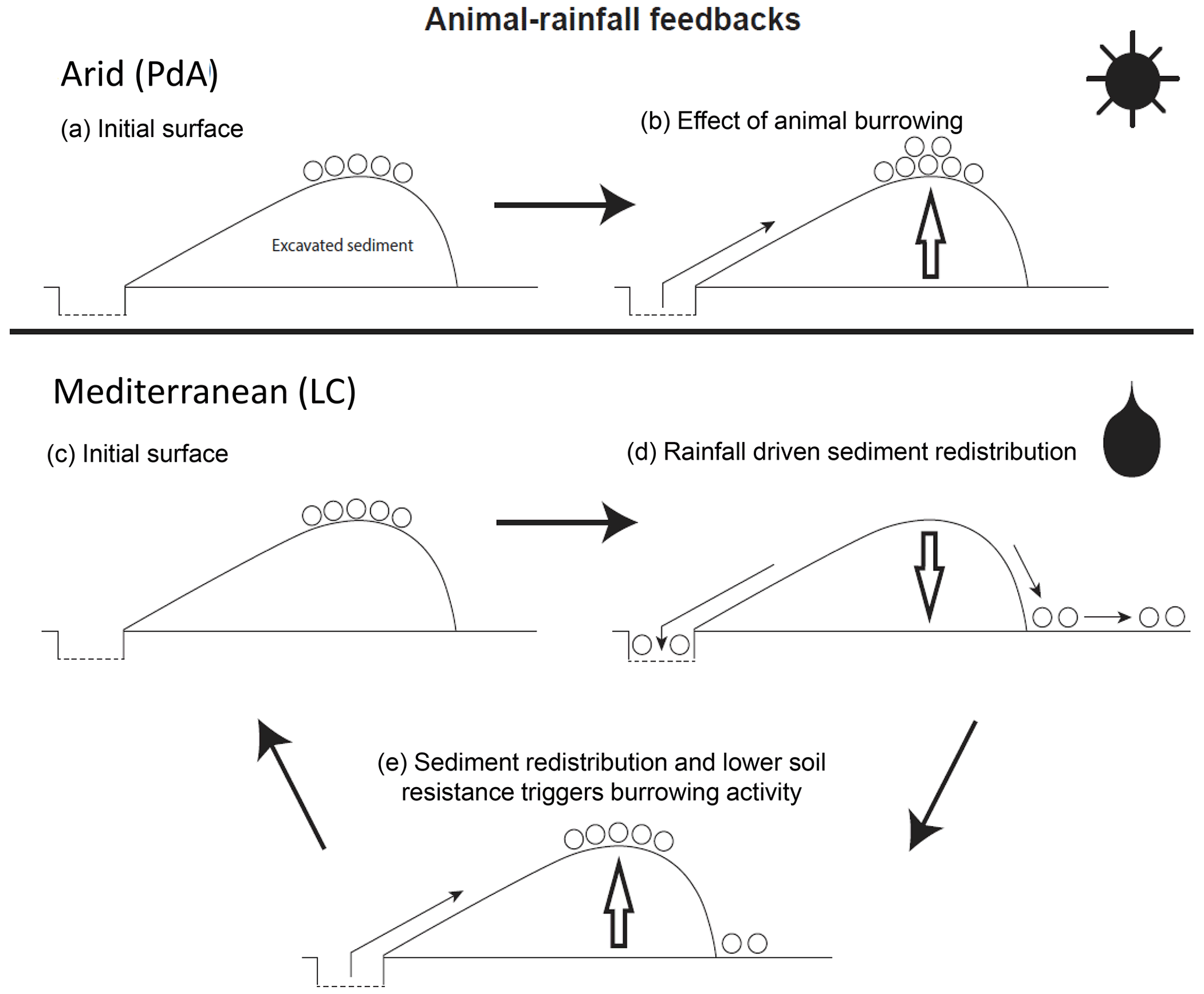
Figure 9 Scheme of animal-driven and rainfall-driven sediment redistribution processes in both investigated climate zones. Panel (a) describes the initial surface of the burrow before the start of a sediment redistribution process, and panel (b) describes the animal excavation process in the arid climate zone. Here, due to rarely occurring rainfall events, sediment redistribution is mostly controlled by the animal burrowing activity. Panel (c) describes the initial burrow surface in the Mediterranean climate zone, panel (d) describes the process of sediment redistribution during a rainfall event, and panel (e) describes the subsequent animal burrowing activity. Burrowing is triggered by decreased soil resistance due to the increased soil moisture after rainfall and by sediment accumulation within the burrow's entrance. Burrowing activity leads to a new supply of sediment being excavated to the surface. In the Mediterranean climate zone, sediment redistribution is controlled by both animal burrowing activity and rainfall. The alternating excavation and erosion processes ultimately lead to an increase in redistribution rates.

Our results indicate an up to 338 % increase in the sediment volume redistributed during rainfall events measured within burrows when compared to burrow-embedded areas. In contrast to our result, the maximum increase estimated in previous studies was 208 % (Table A6, Imeson and Kwaad, 1976). The two climate zones also show different patterns. In the Mediterranean climate, the contribution of animal (vertebrate) burrowing activity appears larger than previously observed by using field methods such as erosion pins or splash traps (from −3 % to −208 %; see Table A6; Imeson and Kwaad, 1976; Hazelhoff et al., 1981; Black and Montgomery, 1991). In contrast, in arid PdA, our study found a much smaller increase (40 %, Table A6) in the sediment volume redistributed during rainfall events measured within burrows when compared to burrow-embedded areas. This is lower than previously estimated (125 %; see Table A6; Black and Montgomery, 1991). However, only one rainfall event above 0.2 mm d⁻¹ occurred during our monitoring period. Hence, we conclude that the contribution of the burrowing activity of animals to hillslope sediment transport is much larger in areas with frequent rainfall events than previously thought, while it has been realistically estimated by previous studies for areas with rare rainfall events (Table A6).

Magnitudes of sediment volume redistributed within burrows similar to our results were previously obtained only in studies applying rainfall simulators. These studies estimated an increase in the volume of sediment redistributed during rainfall events, measured within burrows when compared to burrow-embedded areas, to be between 205 % and 473 % (Table A6, Li et al., 2018; Chen et al., 2021). However, a rainfall simulator can only provide data on surface processes within a plot of a few square meters in size and under ideal laboratory conditions while ignoring the uphill microtopography, vegetation cover and distribution (Iserloh et al., 2013), which were shown to reduce erosion rates. More importantly, the rainfall intensity on hillslopes decreases with (i) the angle of incidence of the rain, (ii) the inclination of the surface, and (iii) the relative orientation of the sloping surface to the rain vector (Sharon, 1980). When simulating a rainfall event with the same rainfall volume as in the field, the rain is induced directly over the treated surface and thus has a higher velocity, which leads to an increased splash erosion than under natural conditions (Iserloh et al., 2013). We thus propose that the rainfall experiments overestimate the erosion rate and that the correct erosion rate can be measured solely under field conditions.

Cumulative sediment redistribution within the burrow roof, mound, and entrance was, on average, 28 % lower than cumulative sediment redistribution only within the mound and the burrow roof (Fig. A7). These results suggest that 28 % of the eroded sediment from animal mounds and burrow roofs is re-accumulated within the burrow entrance during rainfall runoff events, and the remaining 62 % is incorporated into overall hillslope sediment flux. Our numbers contrast with previous studies, which quantified that about 58 % of the sediment excavated by animals will accumulate back in the burrow entrance and only 42 % is incorporated to downhill sediment flux (Andersen, 1987; Reichman and Seabloom, 2002). Hence, our results not only indicate higher redistribution rates within burrows by burrowing animals but also point to a much higher supply of sediment for the downhill sediment flux than previously thought.

Our cost-effective ToF device provides data on surface changes at a high spatiotemporal resolution. The high temporal resolution was able to unravel ongoing low-magnitude but frequent animal excavation and erosion processes. The high spatial resolution enabled us to estimate the exact volume of sediment fluxes from the burrows downhill. The results presented here indicate that the contribution of burrowing animals on the burrow and hillslope scales was much higher than previously assumed. Our results can be integrated into long-term soil erosion models that rely on soil processes and improve their accuracy by including animal-induced surface processes on microtopographical scales in their algorithms.

Appendix A

Table A1 List of abbreviations.

Table A2 Number of usable scans for each camera.

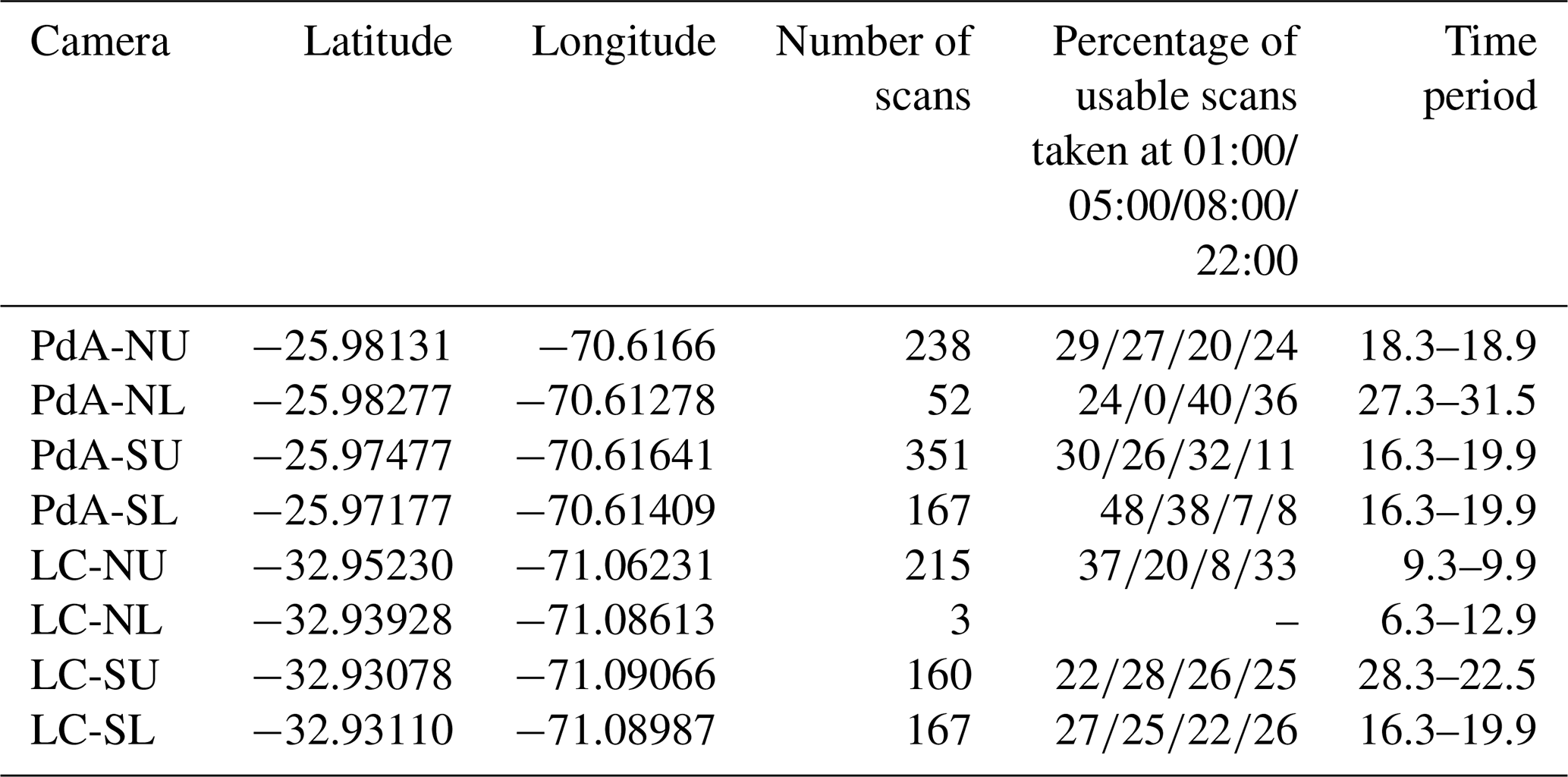
Table A3 Summary of the volume of redistributed sediment according to area and disturbance type. Vol_exc describes the volume of the sediment excavated by the animals. Vol_burrow describes the volume of the sediment redistributed during rainfall events within burrows. Vol_add describes the difference in redistributed sediment volume within burrows and the burrow-embedded area during rainfall.

Table A4 Summary of the volume of redistributed sediment, according to area and disturbance type. Vol_exc describes the volume of the sediment excavated by the animals. Vol_burrow describes the volume of the sediment redistributed during rainfall events within burrows. Vol_add describes the difference in redistributed sediment volume within burrows and burrow-embedded areas during rainfall.

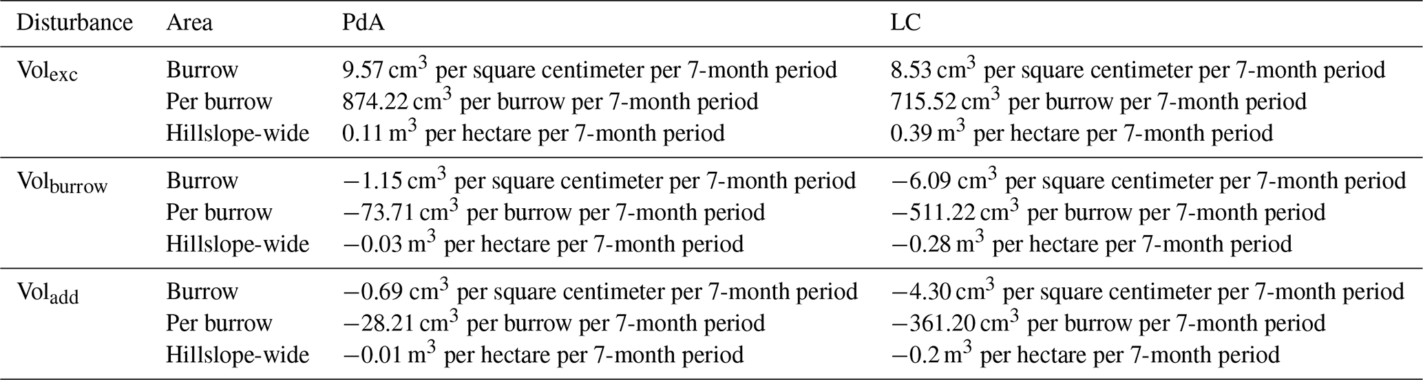
Table A5 Review of studies that used laser scanners for the estimation of surface processes. NA stands for no data available.

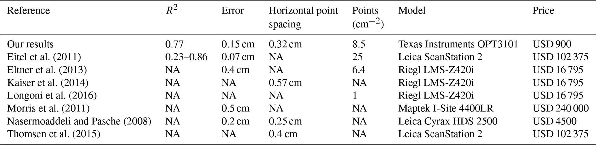
Table A6 Review of studies that estimated the sediment redistribution within burrows and burrow embedding areas and the proposed impact. NA stands for data not available.

Table A7 Review of studies that estimated the sediment redistribution within burrows, average burrow density as found in the literature, and area-wide yearly contribution of burrowing animals to sediment redistribution.

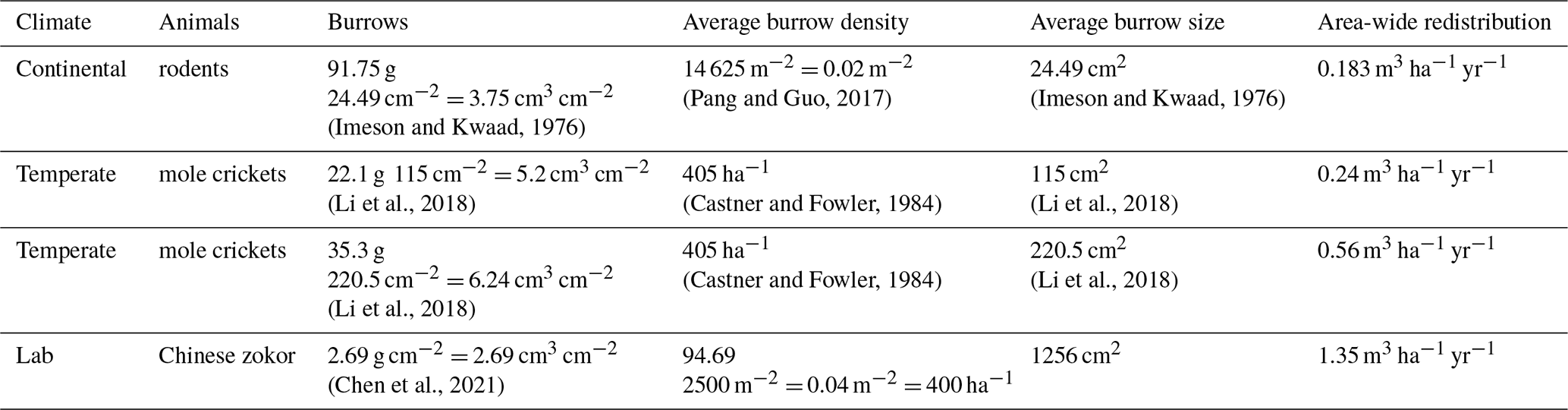
Table A8 Review of studies that estimated the volume of sediment excavated by burrowing animals.

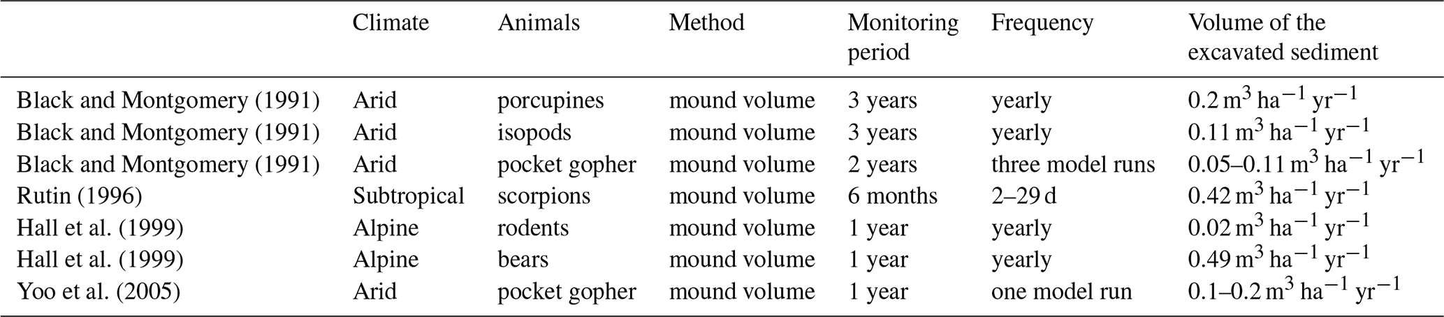
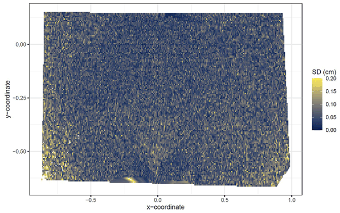
Figure A1 Standard deviation of the z coordinate of five unprocessed scans shown for the camera on the north-facing upper hillslope. SD is standard deviation. The error increases with distance from the camera nadir point. The standard deviation was calculated from the scans before any corrections.

Figure A2 Delineation of the areas. The point of origin of the coordinate system is at the camera nadir. Depth is the distance between the surface and the camera. The red lines show the outline of the burrow entrance. The green lines show the outline of mound. The oranges lines show the outline of burrow roof. The area that is not outlined is burrow-embedded area. The examples shown are as follows: (a) LC-NU, (b) LC-NL, (c) LC-SU, (d) LC-SL, (e) PdA-NU, (f) PdA-NL, (g) PdA-SU, and (h) PdA-SL.

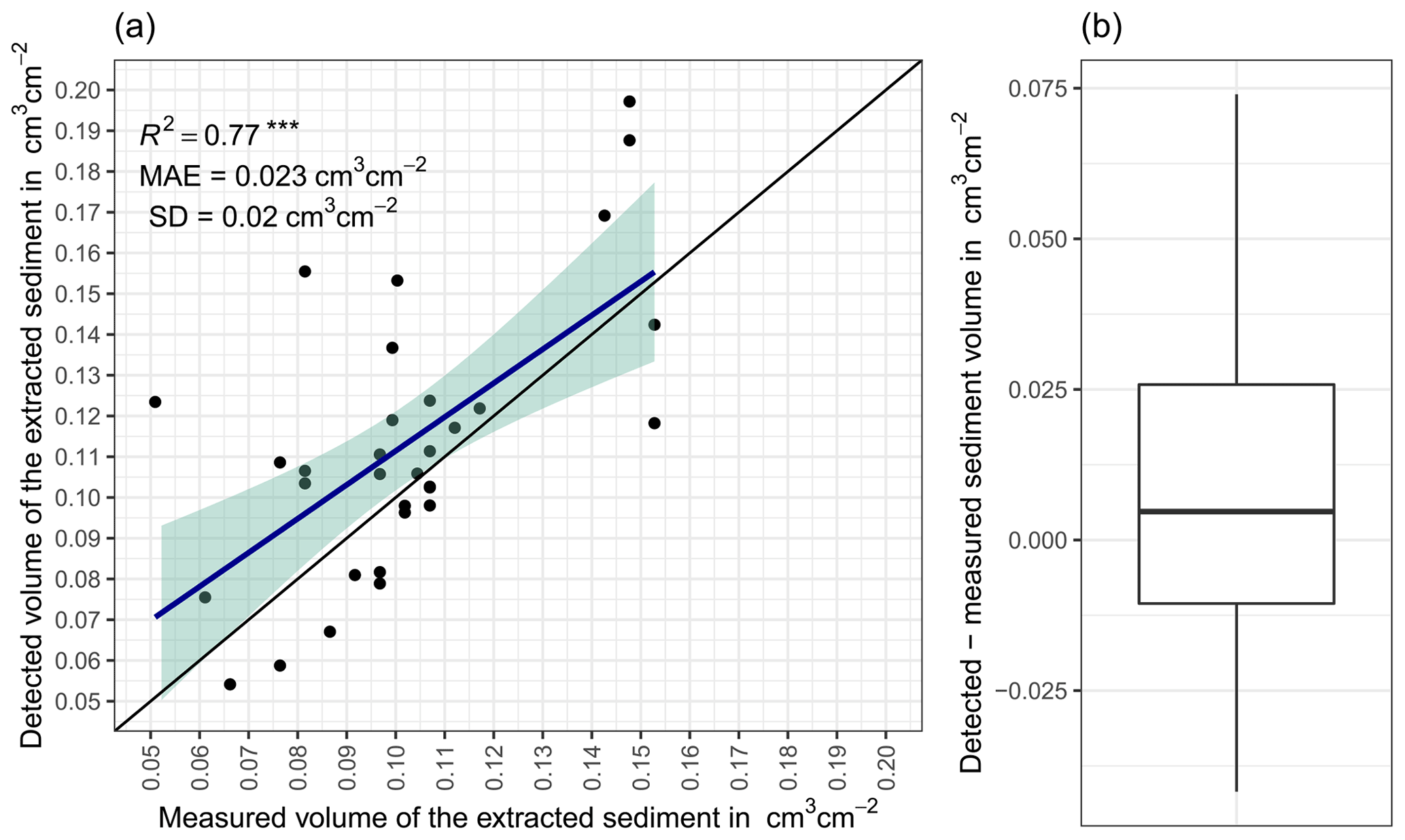
Figure A3 (a) Estimation of time-of-flight camera accuracy based on averaging two surface scans before and after the sediment extraction under controlled conditions. The x axis shows the exact sediment volume measured with a cup. The y axis represents the volume of the sediment calculated from the camera scans (according to Eq. 4). The blue line is the linear regression calculated from the measured and detected volume. The green shadow shows the confidence interval of 95 % for the linear regression slope. MAE is the mean absolute error, SD is standard deviation, and R² is the coefficient of determination. (b) Measured sediment volume subtracted from the detected sediment volume for all measurements. ${}^{***}p\le \mathrm{0.001}$.

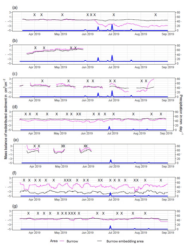
Figure A4 Sediment mass balance for the period of 7 months shown separately for burrows and burrow-embedded areas as measured by the cameras: (a) LC-NU, (b) LC-SU, (c) LC-SL, (d) PdA-NU, (e) PdA-NL, (f) PdA-SU, and (g) PdA-SL. For definitions of the abbreviations, see Table A1.

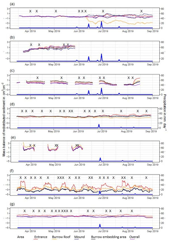
Figure A5 Sediment mass balance for the period of 7 months shown separately for all delineated areas as measured by the cameras: (a) LC-NU, (b) LC-SU, (c) LC-SL, (d) PdA-NU, (e) PdA-NL, (f) PdA-SU (g) PdA-SL. For definitions of the abbreviations, see Table A1.

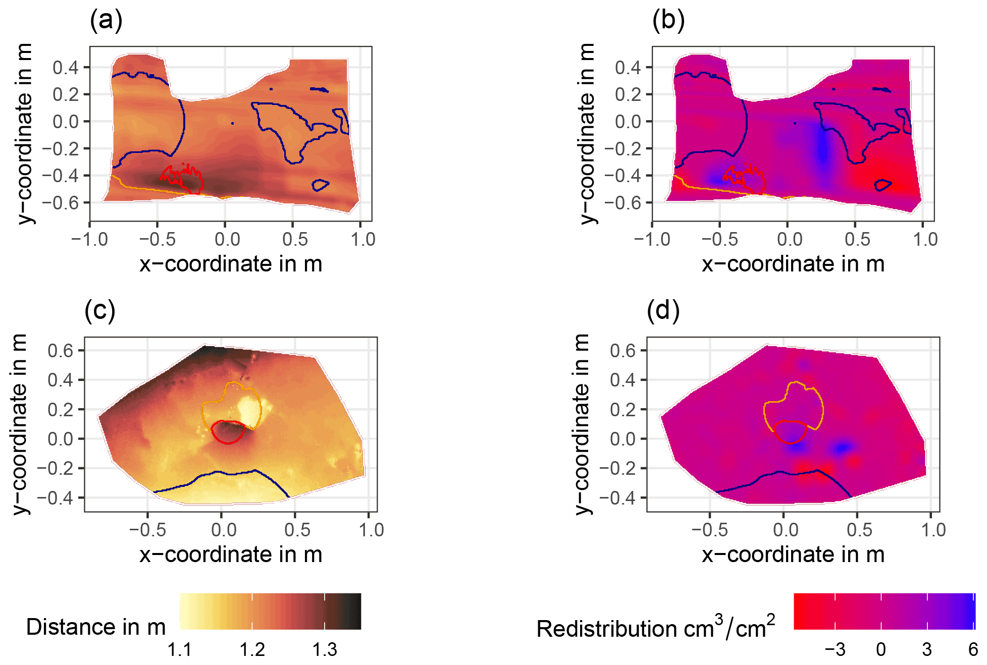
Figure A6 Examples of surface scans showing the digital surface model (DSM) before a rainfall event (a, c) at two camera locations at La Campana and the calculated volume of redistributed sediment (b, d) after the rainfall event: (a) DSM of a scan from the camera on the north-facing upper hillslope at La Campana, (b) detected sediment redistribution (cm³ cm⁻²) on the north-facing upper hillslope at La Campana after a rainfall event of 17.2 mm d⁻¹;, (c) DSM of a scan from the camera on the south-facing upper hillslope at La Campana, and (d) detected sediment redistribution (cm³ cm⁻²) on the south-facing upper hillslope after a rainfall event of 17.2 mm d⁻¹. The red lines show the outline of the burrow entrance. The blue lines show the outline of mound. The orange line shows the outline of the burrow roof. The area that is not outlined is the burrow-embedded area. Redistribution is the volume of the redistributed sediment (per cm³ cm⁻²), either accumulated (positive value) or eroded (negative value). After the rainfall events, sediment mostly accumulated within the burrow entrance or near mounds and eroded from burrow roofs and mounds.

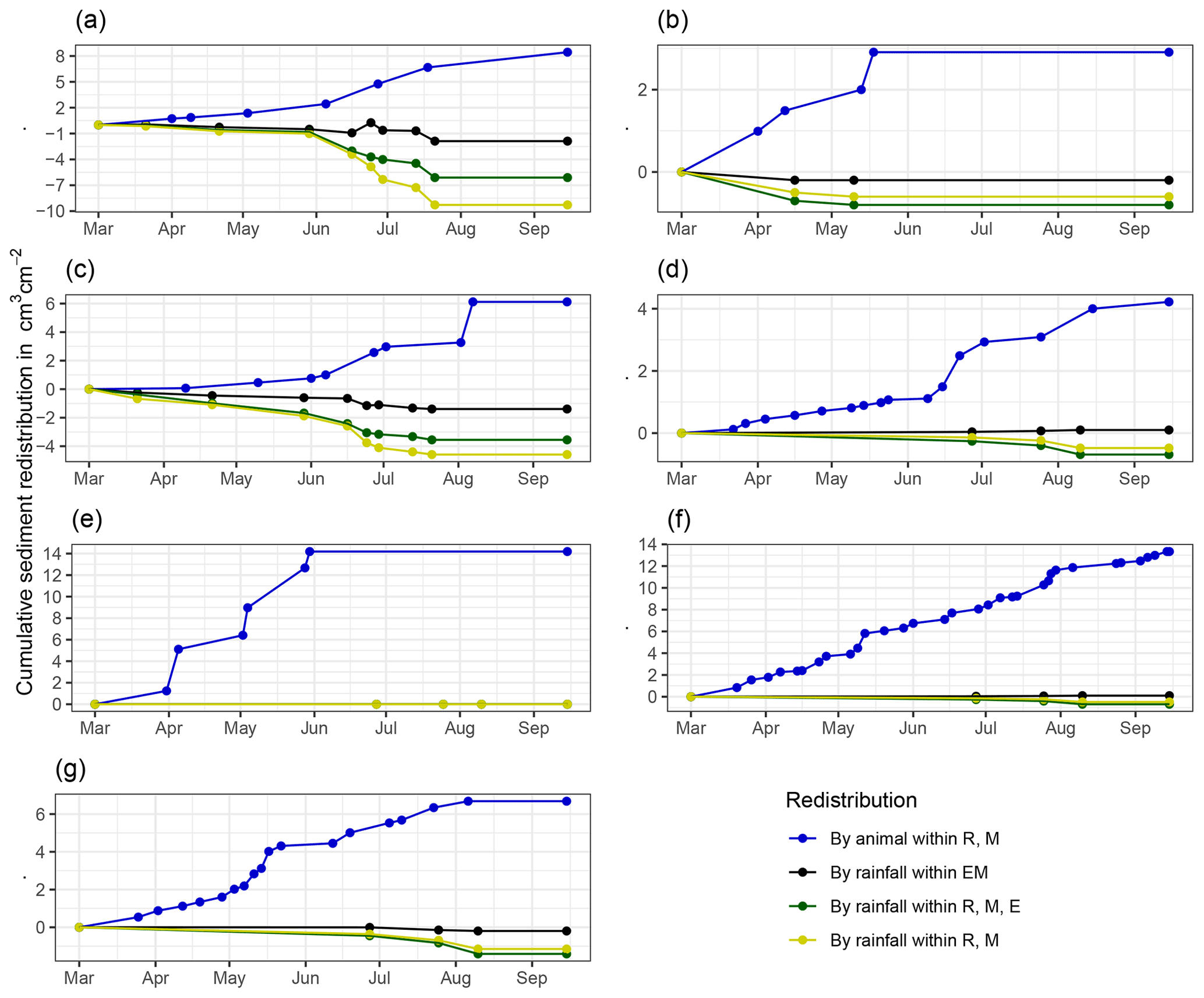
Figure A7 Cumulative volume of redistributed sediment for all cameras. Positive values indicate sediment accumulation. Negative values indicate sediment erosion. Whiskers are the median sediment redistribution. E is the burrow entrance. M is the mound. R is the burrow roof. EM is the burrow-embedded area. LC is the Mediterranean climate zone. PdA is the arid climate zone: (a) LC-NU, (b) LC-SU, (c) LC-SL, (d) PdA-NU, (e) PdA-NL, (f) PdA-SU, and (g) PdA-SL. For definitions of the abbreviations, see Table A1.

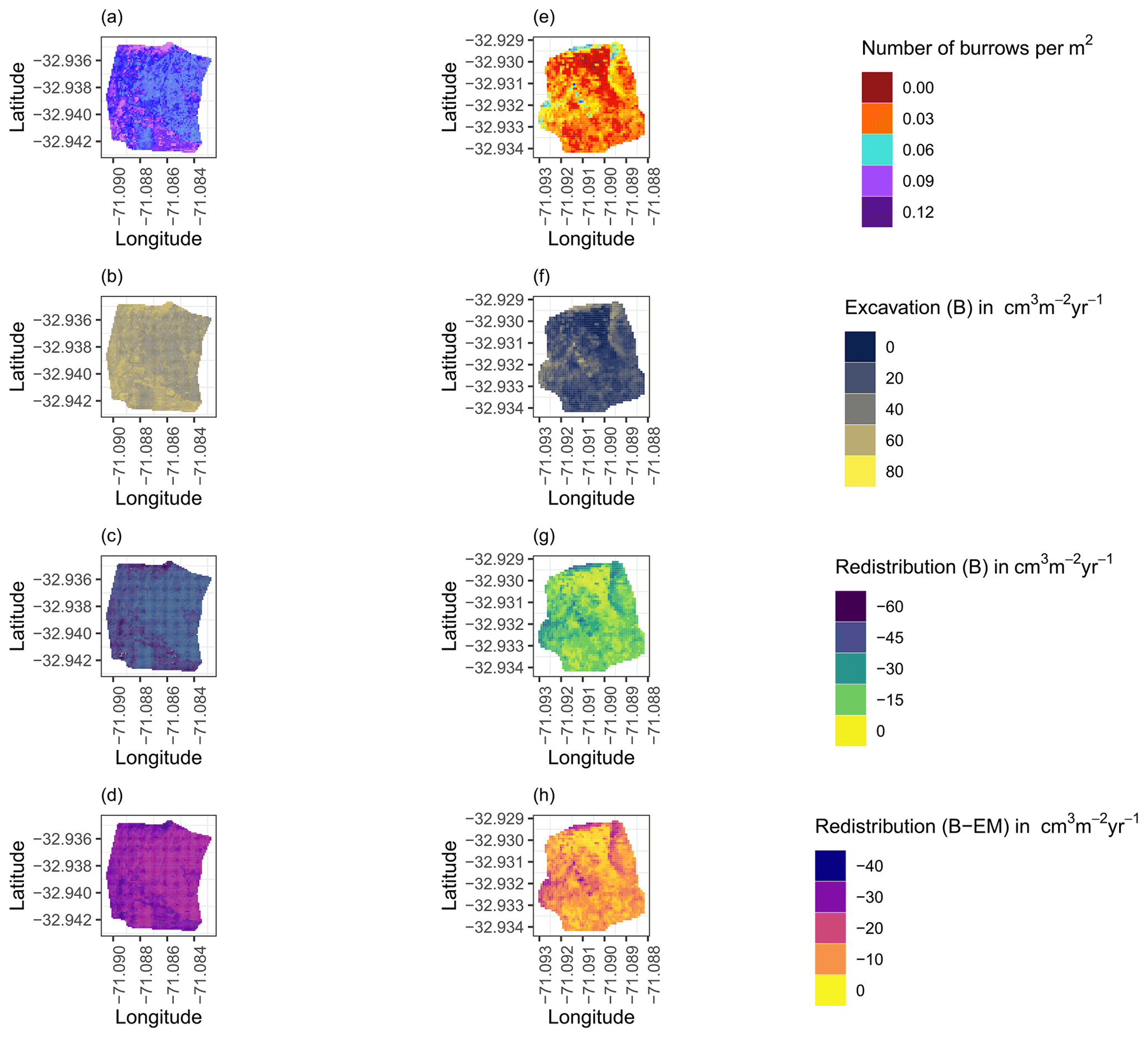
Figure A8 Hillslope-wide volume of redistributed sediment for a time period of 1 year at LC for the (a–d) north-facing hillslope and (e–h) south-facing hillslope. (a, e) Density of burrows as estimated by Grigusova et al. (2021). (b, f) Volume of the sediment excavated by the animals. (c, g) Volume of the sediment redistributed during rainfall events within burrows. (d, h) Volume of additionally redistributed sediment during rainfall events due to the presence of the burrows. The values were calculated per burrow as stated in Sect. 3.7 by subtracting the sediment volume redistributed within burrows from the sediment volume redistributed within burrow-embedded area and then upscaled. B stands for burrow, and EM stands for burrow-embedded area.

Figure A9 Hillslope-wide volume of redistributed sediment for a time period of 1 year at PdA for the (a–d) north-facing hillslope and (e–h) south-facing hillslope. (a, e) Density of burrows as estimated by Grigusova et al. (2021). (b, f) Volume of the sediment excavated by the animals. (c, g) Volume of the sediment redistributed during rainfall events within burrows. (d, h) Volume of additionally redistributed sediment during rainfall events due to the presence of the burrows. The values were calculated per burrow as stated in Sect. 3.7 by subtracting the sediment volume redistributed within burrow from the sediment volume redistributed within burrow embedding area and then upscaled. B stands for burrow, and EM stands for burrow-embedded area.