the Creative Commons Attribution 4.0 License.
the Creative Commons Attribution 4.0 License.
 | 27 Apr 2022
Convolutional neural networks for image-based sediment detection applied to a large terrestrial and airborne dataset
Xingyu Chen
Marwan A. Hassan
Image-based grain sizing has been used to measure grain size more efficiently compared with traditional methods (e.g., sieving and Wolman pebble count). However, current methods to automatically detect individual grains are largely based on detecting grain interstices from image intensity which not only require a significant level of expertise for parameter tuning but also underperform when they are applied to suboptimal environments (e.g., dense organic debris, various sediment lithology). We proposed a model (GrainID) based on convolutional neural networks to measure grain size in a diverse range of fluvial environments. A dataset of more than 125 000 grains from flume and field measurements were compiled to develop GrainID. Tests were performed to compare the predictive ability of GrainID with sieving, manual labeling, Wolman pebble counts (Wolman, 1954) and BASEGRAIN (Detert and Weitbrecht, 2012). When compared with the sieving results for a sandy-gravel bed, GrainID yielded high predictive accuracy (comparable to the performance of manual labeling) and outperformed BASEGRAIN and Wolman pebble counts (especially for small grains). For the entire evaluation dataset, GrainID once again showed fewer predictive errors and significantly lower variation in results in comparison with BASEGRAIN and Wolman pebble counts and maintained this advantage even in uncalibrated rivers with drone images. Moreover, the existence of vegetation and noise have little influence on the performance of GrainID. Analysis indicated that GrainID performed optimally when the image resolution is higher than 1.8 mm pixel−1, the image tile size is 512×512 pixels and the grain area truncation values (the area of smallest detectable grains) were equal to 18–25 pixels.
- Article
(7253 KB) - Full-text XML
- BibTeX
- EndNote


Sediment grain size and its spatial variability are fundamental in river dynamics (e.g., sediment transport, channel evolution), ecological studies (e.g., aquatic habitat, fishery) and river restoration engineering. However, the measurement of grain size has been time-consuming and laborious especially in mountain rivers due to the wide range of grain size classes, diverse grain lithology, the hiding of grains, diverse structures and the influence of organic materials. The most widely used grain sizing method is sieving (Kellerhals and Bray, 1971) which is used as a benchmark to other methods when reliable sediment samples are able to be collected (Church et al., 1987). Wolman (1954) proposed a pebble count method (Wolman method) that samples a minimum of 100 pebbles from the riverbed surface with a grid-based system. Limited to material > 8 mm (Kellerhals and Bray, 1971), the Wolman method has been especially popular in the field due to the limited equipment required and its benefit of reducing sampling times while providing a relatively valid estimation of reach-scale grain size distribution. Since then, various versions of the Wolman method have been proposed with different approaches to collecting stones such as the random walk approach for particle collection (Leopold, 1970), superimposing gravel templates upon the sedimentological unit for reduced operator error (Bunte and Abt, 2001) and image-based Wolman method analysis (Hassan et al., 2020; An et al., 2021).
Since the 1970s, advances in high-resolution photography have provided scientists the opportunity to estimate sediment grain size in river beds from images, largely reducing sampling time for large-scale field surveys compared with sieving and Wolman methods (Church et al., 1987; Adams, 1979). However, the development of such methods to measure grain size from images has been challenging as early studies relied on the laborious manual identification of grain boundaries on vertical images (Adams, 1979; Ibbeken and Schleyer, 1986) and only within the past 20 years has there been the development of automated grain sizing algorithms (Graham et al., 2005b; Buscombe et al., 2010; Rubin, 2004). Generally, image-based automated grain sizing methods can be classified from percentile-based to object-based methods (Buscombe, 2020). Percentile-based methods (Carbonneau et al., 2004; Rubin, 2004; Buscombe, 2020; Buscombe et al., 2010) estimate grain size distribution based on statistical analysis of image intensity and texture through pixel-wise simple autocorrelation algorithms (Rubin, 2004), grain size prediction as a function of both local image texture and semi-variance (Carbonneau et al., 2004), spectral decomposition of an image (Buscombe et al., 2010) and convolutional neural networks (CNN; Buscombe, 2020; Mueller, 2019; Lang et al., 2021). Object-based methods (Sime and Ferguson, 2003; Detert and Weitbrecht, 2012; Graham et al., 2005a, b; McEwan et al., 2000) apply sequences of grain separation algorithms to detect grain interstices and identify each individual grain on the bed. McEwan et al. (2000) applied an automatic edge-detection algorithm on digital elevation models (DEMs) of grain surfaces generated by laser scanning and reported promising grain size measuring results. Sime and Ferguson (2003) presented a modified edge-detection algorithm which combined both edges seeding and partial watershed segmentation algorithms. Graham et al. (2005a, b) proposed a double threshold interstice-detection approach in which the threshold levels to detect grain interstices were initially defined based on image intensity distribution and further refined through a bottom-hat filter. Based upon this approach, Detert and Weitbrecht (2012) proposed an enhanced grain detecting model (named BASEGRAIN) which applies a five-step image-processing procedure to separate grains on the bed.
As noted by several researchers (e.g., Carbonneau et al., 2004; Graham et al., 2010; Buscombe, 2020), object-based methods require sophisticated object segmentation algorithms and theoretically cannot be used on grains smaller than 1 pixel; however, object-based methods can provide grain scale information on spatial variability which is essential in not only predicting but also understanding the processes of flow resistance (Chen et al., 2020), sediment transport (Yager et al., 2018) and aquatic habitat (Reid et al., 2020). The BASEGRAIN model developed by ETH Zurich is a state-of-the-art, object-based grain sizing software, but it requires extensive parameter tuning (the model contains more than 40 adjustable parameters and 7 key parameters) and a significant level of expertise to be applied to suboptimally captured images. Moreover, the model only focuses on detecting edges and as such performs poorly in fluvial environments where dense organic debris, various sediment lithology and nonuniform lighting are present in the photo (Detert and Weitbrecht, 2020). The limitations of BASEGRAIN in these suboptimal environmental conditions can be overcome using CNN which have been extensively used in computer vision (Krizhevsky et al., 2012) and biomedical applications (Ronneberger et al., 2015). Through repeated convolutions and pooling on the input images, CNN can automatically capture not only object edges but also high-level features such as shape, color and texture (Buscombe, 2020). In addition, with nonlinear activation functions (e.g., sigmoid) in every neuron, the network is capable of learning the nonlinearity of grain features under diverse environments. When trained with large sets of images, CNN techniques have proven to be a robust tool for object classification and identification (He et al., 2016) even when applied to suboptimally conditioned images (e.g., nonuniform lighting, noise due to organic debris).
For image segmentation tasks, one of the most widely used CNN architectures is U-Net (Ronneberger et al., 2015), which was designed to separate individual cells in biomedical images. U-Net has been successfully applied to solve many problems such as multi-organ segmentation (Oktay et al., 2018), detection of lung abnormalities (Kohl et al., 2018) and autonomous driving (Tran and Le, 2019). The detection of grains is different with the tasks above in regards to the wide range of grain size classes, diverse grain lithology and the hiding of the grains, and the potential of U-Net to detect sediments in diverse fluvial environments has not yet been studied (Mueller, 2019). For field grain size measurements, especially in watershed-scale drone surveys, the size of large boulders to be detected can be several magnitudes larger than the size of fine sediments; however, the scale and resolution of input images to U-Net are limited by GPU memory and model complexity. As such, predictive errors arise when splitting the large images into sub-tiles for predicting fine sediments. Moreover, inter-granular noise is introduced due to the diverse lithology and weathering, for example, the internal texture for weathered rock tends to be falsely detected as grain interstices. As a result, how can we reduce errors when applying U-Net for grain detection in a diverse range of fluvial environments? How does image resolution and image tile size influence the predictive ability of U-Net? What is the size of the smallest detectable grain unit for U-Net? These questions have yet to be answered. Therefore, it is of great value to develop a U-Net-based model for grain size measurement in diverse fluvial environments.
In this paper, we propose a model (GrainID) based on U-Net with an overlap-tile strategy to detect grain size from images in a diverse range of fluvial environments. To achieve our goal, we (i) compiled a large dataset of grain images containing more than 125 000 grains in a diverse range of fluvial environments and trained GrainID with the datasets, (ii) compared the results of GrainID with sieving, manual labeling, Wolman and BASEGRAIN methods, (iii) tested the performance of GrainID for uncalibrated rivers with airborne photos and (iv) evaluated the influence of vegetation, inter-granular noise, image tile size and resolution on model performance.
The datasets (84 flume, 118 field photos) cover a wide range of fluvial environments and include a variety of field site and flume experiment images. As shown in Table 1, the datasets were grouped into three subsets according to sediment and channel conditions: (1) flume channel (84 photos; photo size ∼ 0.2 m × 0.2 m); (2) forested mountain rivers (70 photos; photo size ∼ 1 m × 1 m); and (3) sparsely vegetated large rivers (6 photos; photo size ∼ 20 m × 20 m). To train the machine learning model to better distinguish sediments from field environmental elements (e.g., cohesive sands, wood, vegetation and water) and improve the model robustness, we specifically collected 42 field photos primarily consisting of various environmental elements with limited sediment grains in the images.
Table 1Description of datasets.
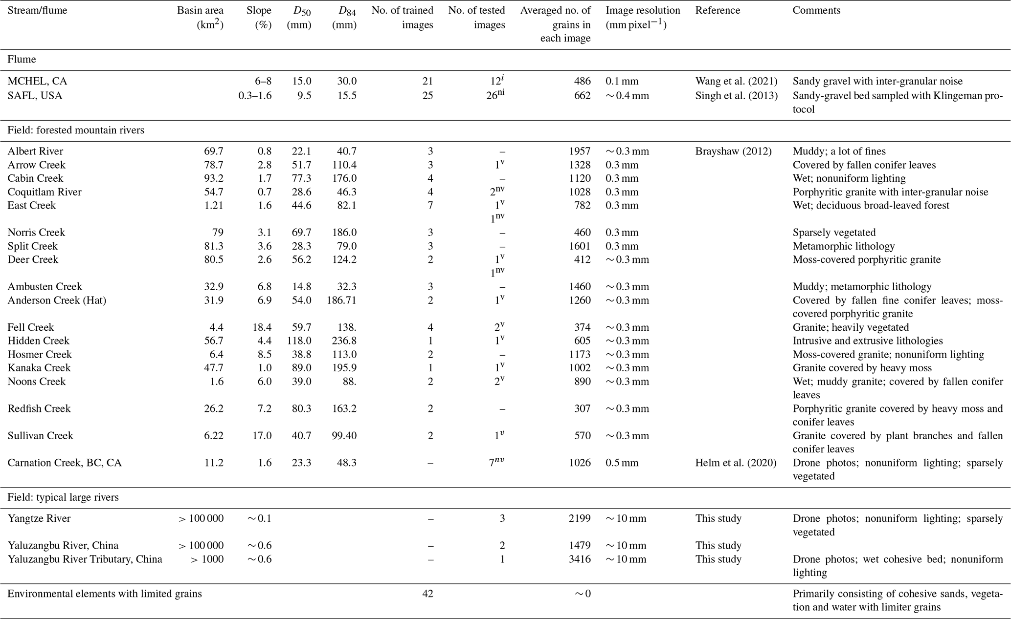
v tested images with vegetation. nv tested images without vegetation. i tested images with inter-granular noise. ni tested images without inter-granular noise.
2.1 Flume channel
The first flume set (SAFL dataset) was collected in a riffle-pool experiment (Fig. 1a; flume size: 2.8 m × 55 m) carried out in the St. Anthony Falls Laboratory (SAFL) at the University of Minnesota (Singh et al., 2013). The channel bed samples were primarily composed of a sandy-gravel mixture created by adding sand to the clean gravel mixture and turning the bed over. Bed surface samples were then collected and sieved using the Klingeman Sampling protocol (Kondolf, 2000; Klingeman and Emmett, 1982). The second flume set (MCHEL dataset) consisted of 33 flume photos taken from a step-pool experiment (flume size: 0.4 m × 5 m) carried out in the Mountain Channel Hydraulic Experimental Laboratory (MCHEL) at The University of British Columbia (Fig. 1b). A nonuniform sediment mixture with a wide grain size distribution between 0.5 and 64 mm (measured by sieving) was used. The sediments in MCHEL are painted in different colors to classify different grain sizes, but the issue of wearing on the grain surface introduces inter-granular noise like the noise introduced by different grain lithologies in the field.
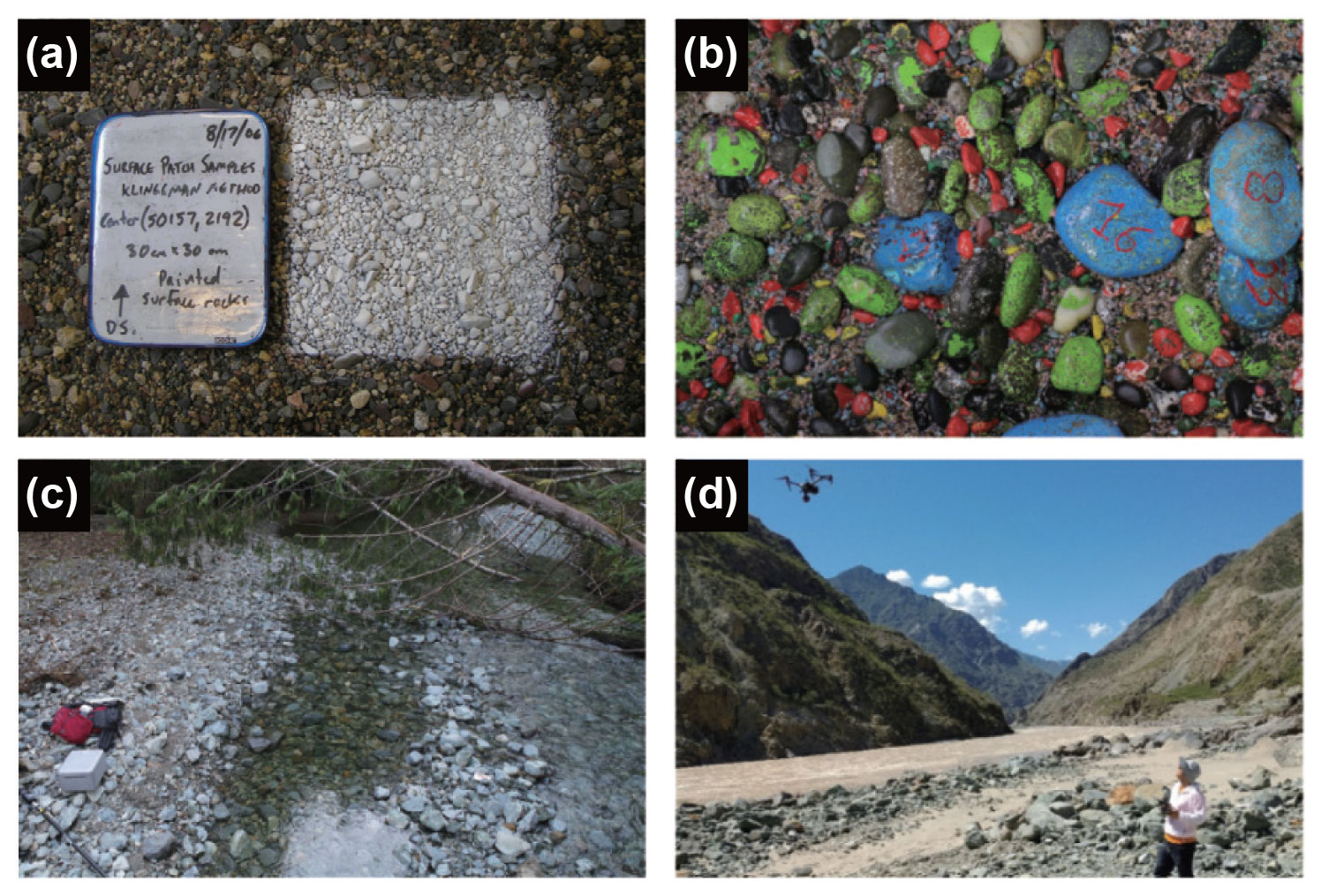
Figure 1Four typical environments in our datasets: (a) bed sample collected in SAFL; (b) step-pool channel bed in MCHEL; (c) Carnation Creek; and (d) Upper Yangtze River.
2.2 Forested mountain rivers
70 grain photos (Brayshaw, 2012; Helm et al., 2020) were collected in 18 small forested gravel-bed rivers (basin area < 100 km2; Fig. 1c) in British Columbia, Canada. Visual assessments suggest that a large proportion of the channels were hidden beneath a dense forest canopy composed of both coniferous and deciduous tree species (Fig. 1c), with a channel slope ranging from 0.007 to 0.184, and the sediments cover a wide range of sedimentary, metamorphic, intrusive and extrusive lithologies (Brayshaw, 2012; Hassan et al., 2014). The grain size information in Table 1 for forested rivers was calculated by Brayshaw (2012) using the Digital Gravelometer software proposed in Graham et al. (2005b).
Sparsely vegetated large rivers: Six unmanned aerial vehicle photos were collected by our research group of two large mountain rivers in China: Upper Yangtze River (Fig. 1d) and Yaluzangbu River. The photos were taken along the riverbank in which they were influenced by the presence of water, waves and cohesive sediments. There was sparse vegetation in the images and the sediments were primarily composed of moderately weathered silicate mineral.
The datasets of 202 images were randomly split into two subsets (Table 1): a training subset (for training and validation) with 136 images and a test subset with 66 images. The training subset was further split into training and validation datasets with a 5-fold cross-validation method during the model training process, and the test subset was a true holdout set to test the model's predictive ability with new images. To evaluate the influence of vegetation and inter-granular noise on model performance, the test subset was further grouped based on the presence of vegetation and inter-granular noise, in which GrainID, BASEGRAIN and the Wolman method were tested for each of the data groups. As shown in Table 1, the tested images with/without vegetation were marked with the superscript v/nv while the tested images with/without inter-granular noise were marked with the superscript i/ni.
3.1 Manual labeling
Manual labels were created for all grain images as baseline labels to train and evaluate the methods. Manual labeling was chosen as it is a robust method when applied to diverse fluvial environments due to its basis on human cognitive analysis, and it has been widely used as baseline method for grain detection studies (Sime and Ferguson, 2003; Graham et al., 2005a). Figure 2a–d are the examples of two field images and the corresponding manual labels. Figure 2a shows a bed with vegetation (Anderson Creek), and Fig. 2c shows a bed without vegetation but with inter-granular noise due to grain lithology. The grains are marked as white pixels isolated from each other and the interstices are marked as black pixels (Fig. 2b, d). For grains covered by vegetation, only the exposed part was labeled, and grains with an area of 23 pixels were chosen as the smallest grains to be labeled (Detert and Weitbrecht, 2012). As shown in Fig. 2, the images are large enough to capture the grain size distribution even with the presence of vegetation in the image. A total of 128 461 grains were marked for the entire dataset of 202 images (67 612 in the training datasets, 60 849 in the test datasets) by two operators, in which operator 1 created 170 images and operator 2 created 33 images. To ensure the quality of manual labels, a cross-check labeling workflow was used. When an operator finished labeling an image, the labels would be double-checked by the other operator (the inspector). Missing grains found by the inspector would be confirmed by both operators, and only those consensus “missing grains” would be added to labels.
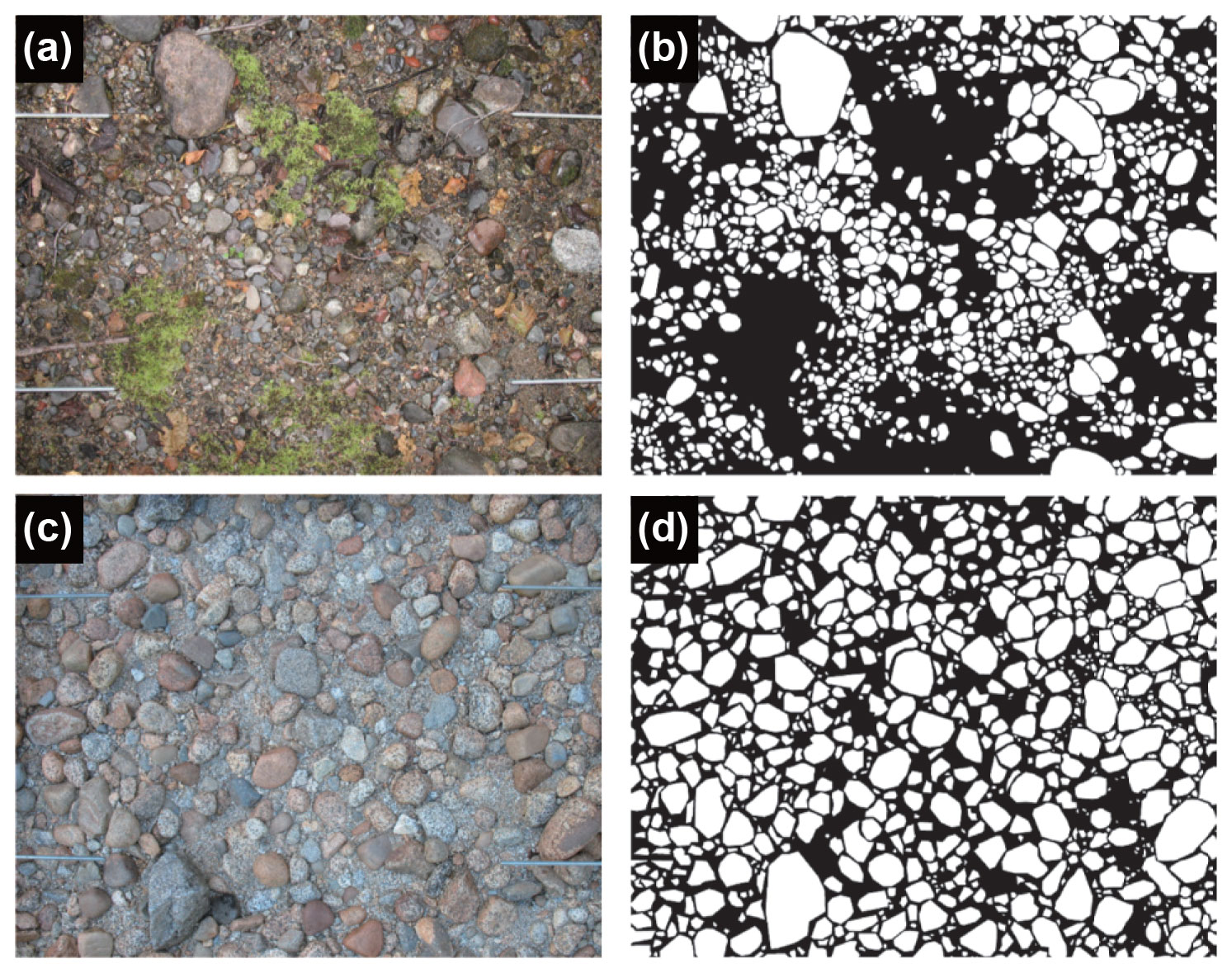
Figure 2Examples of two field photos and the corresponding manual labels: (a) photo with vegetation from Anderson Creek and (b) the corresponding manual label; (c) photo without vegetation from Coquitlam River and (d) the corresponding manual label.
To explore the consistency in labeling and estimate human related errors, five human operators (including operators 1 and 2) were asked to label a fixed dataset of 12 photos containing 8000+ grains in diverse fluvial environments. The photos are selected from Table 1, in which 6 are from forested mountain rivers, 3 are from the SAFL dataset (Singh et al., 2013), 2 are from the MCHEL dataset and 1 is an airborne photo from Yaluzangbu River.
Boxplots were applied to describe the variation of predicted grain size between the operators. The boxplot displays the five-number summary of a set of data including the maximum, third quartile, median, first quartile and minimum (from top to bottom). Figure 3 shows the boxplot of normalized grain size Dnormalized (Dnormalized= () for different grain percentiles and different operators, in which D is the predicted grain size for a manual label, Dmean is the mean grain size value of 12 photos chosen for analysis and DSD is the standard deviation of grain size value of the 12 photos. As shown in Fig. 3, the five operators showed consistent median, first/third quantile and maximum/minimum values for all Dnormalized statistics and all grain percentiles, indicating the consistent predictive ability of the five operators for grains in diverse environments. An exception is D50, in which operators 2 and 5 showed a higher maximum value of Dnormalized than the other three operators. The inconsistency for D50 prediction mainly arises from the predictions for the three photos from the SAFL dataset in which the bed contains a lot of fine grains, and operators 2 and 5 overestimated the D50 by merging fine grains as larger sediments. The analysis suggests that operator 1 produced consistent grain size for all percentiles, but operator 2 may have overestimated D50 for images with fine grains. Overall, the manual labels datasets prepared by operators 1 and 2 were consistent with labels created by human operators.

Figure 3Boxplot of normalized grain size Dnormalized for percentiles Di for five human labeling operators.
3.2 GrainID
3.2.1 Model framework
A model framework (GrainID) to detect grains from images in diverse fluvial environment is introduced in this section. Figure 4a shows the framework of the GrainID model working in its 3-step procedure, and Table 2 lists the detailed description of each processing step. For image pre-processing (step 1), we tried three image filters in the Python Image Processing Library (Pillow; Clark, 2015): “edge enhancement”, “sigmoid contrast”, and “detail”, in which the “sigmoid contrast” filter was chosen for its lower predictive error. Image augmentation (Fig. 4c), a widely used technique for CNN prediction, allowed the network to learn variances in object location, rotation or deformation without the need to see these transformations in the annotated image corpus.
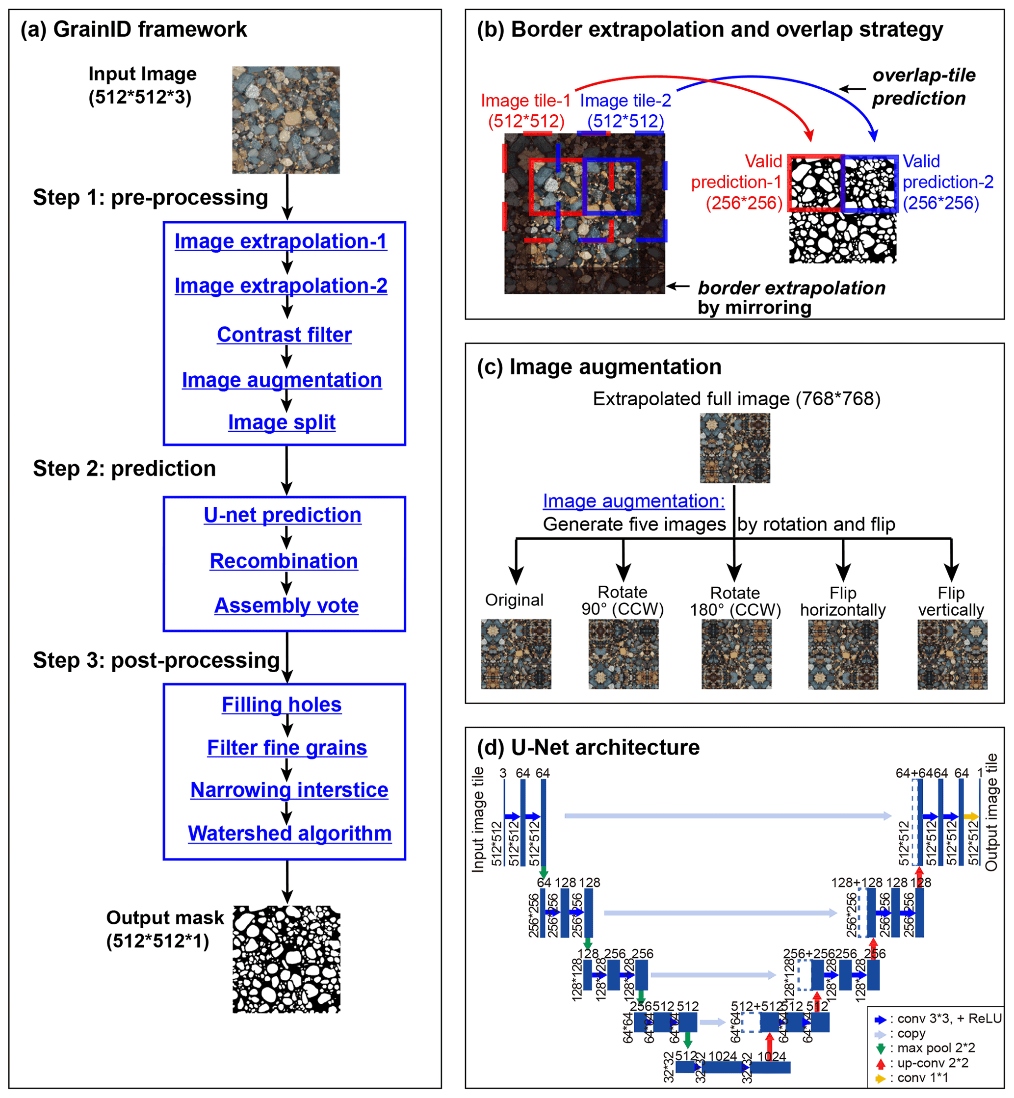
Figure 4Framework and specific algorithms of GrainID: (a) GrainID framework; (b) border extrapolation and overlap-tile prediction; (c) image augmentation; and (d) U-Net architecture adapted from Ronneberger et al. (2015).
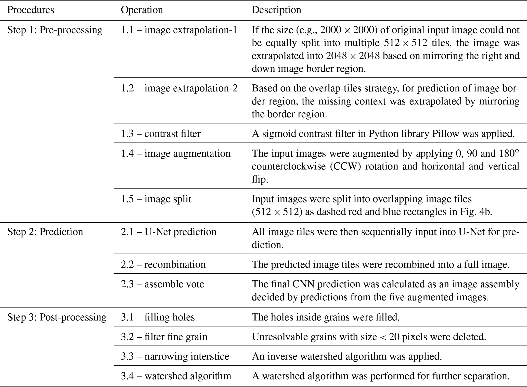
The CNN prediction for the border region of an image is invalid as the convolution used mirroring context rather than real image information of the border for prediction purposes (Ronneberger et al., 2015). As such, errors are introduced when splitting a large photo into many image tiles for U-Net prediction. To solve this problem and achieve seamless prediction, in step “Image extrapolation-2” and “Image split”, we applied an overlap-tile strategy (Ronneberger et al., 2015). The overlap-tile strategy only utilizes the central parts of an image tile to be used for valid prediction. For example (Fig. 4b), for image tiles (dashed red and blue rectangles, 512 × 512 pixels) used for U-Net inputs, only the center parts of U-Net outputs (solid red and blue rectangles, 256 × 256 pixels) were accepted for predictions. To achieve seamless prediction, we created overlapping image tiles for our U-Net inputs as dashed red and blue rectangles in Fig. 4b in step “image split”, and the missing context in the border region was extrapolated by mirroring the border region in step “image extrapolation-2” (shown as a shadow region in Fig. 4b).
In step 2, image tiles created by our overlap strategy were then input into U-Net for prediction. The predictions were then recombined into a full image. The final CNN prediction was calculated as a result assembly decided by predictions of the five augmented images, in which the decision rule was that a pixel will be calculated as an interstice if two or more predictions identify an interstice at that pixel so that the model can detect grain interstice and separate grains as much as possible. Four post-processing algorithms were performed in step 3 in which holes inside grains were filled and grains with area < 20 pixels were filtered. To compensate for the error of wide interstices due to human labeling, the interstices between grains were narrowed for 2 pixels using an inverse watershed algorithm. Finally, to further separate the merged grains, a watershed algorithm was performed based on grain centroid information.
For a predicted image, the a axis (major axis) of a grain was defined as the maximum Euclidean distance between two pixels on the grain boundary, and the b axis (minor axis) was calculated as the maximum intercept to the grain along a line perpendicular to the a axis. Based on the b axis and grid-by-area method (Kellerhals and Bray, 1971), sediment percentiles D5, D16, D50, D84 and D95 were calculated for the results of manual labeling, GrainID and BASEGRAIN. The sediment percentiles of the Wolman method were calculated based on a grid-by-number method equivalent to the grid-by-area method demonstrated by Kellerhals and Bray (1971).
3.2.2 U-Net: a CNN architecture for image segmentation
U-Net, evolved from CNNs, is specifically designed for image segmentation application. As shown in Fig. 4d, the U-shaped model architecture consists of two major paths: the contracting path (left part) and the expansive path (right part). The contracting path, similar to the typical CNN architecture, consists of a sequence of 3×3 convolution layers for feature extraction and 2 × 2 max pooling layers for down-sampling. In the expansive path, every operation consists of a transposed convolution layer for up-sampling and two subsequent 3 × 3 convolution layers, where the transposed convolution layer expands the image and maintains the same connectivity as the regular convolution. With this architecture, U-Net can maintain a consistent image size between the output and input and detect specific objects by doing classification on every pixel.
The U-net was implemented based on the Python library “pytorch” (Paszke et al., 2019). The cross entropy loss function and the stochastic gradient descent were used for model optimization. Model hyperparameters were tuned based on grid searching optimization and 5-fold random cross validation (Goodfellow et al., 2016). The training speed for U-Net is influenced by the number of images in the training datasets, the batch size and the number of training epoch. Given a fixed training dataset, the hyperparameter number of training epoch was tuned first, followed by the learning rate. The optimum batch size depends on GPU memory, and we preferred a larger batch size for faster training speed when several batch size values resulted in a similar error during the cross-validation. The optimized model hyperparameters were: (1) number of training epoch = 150; (2) learning rate = 0.005; (3) batch size = 96; and (4) image tile size = 512. The optimum image tile size was determined based on the analysis in Sect. 5.2.
3.3 Manual sieving, BASEGRAIN and Wolman methods
The model proposed in this paper was compared with the manual sieving, Wolman and BASEGRAIN methods. The three methods were considered because they are widely used and accessible.
The manual sieving method was applied to bed samples from the SAFL dataset. Sediment samples were first weighed for a total mass and then sieved through a sieve set (in mm): 32, 22.6, 16, 11.3, 8, 5.6, 4, 2.83, 2, 1.4 and 1. The sediments of each sieve as well as the fine sediments left in the pan were weighed once again, and the weight percentage of each size fraction were calculated (Singh et al., 2013).
The image-based Wolman method samples 100 grains based on an equidistant grid on the image where the sediment distribution was calculated via a grid-by-number approach that has been applied in much of the literature (e.g., Kellerhals and Bray, 1971; Hassan et al., 2020).
The BASEGRAIN applies a 5-step image processing algorithm to detect grains (Detert and Weitbrecht, 2012): In steps 1–3, the model sequentially applies the (1) double grayscale threshold, (2) morphological bottom-hat transformations and (3) the Canny and the Sobel methods to detect grain interstices. In step 4, an improved watershed algorithm is performed for grain segmentation. In step 5, grains with an area < ∼ 23 pixels are excluded and grain properties (e.g., a-axis, b-axis orientation) are calculated. During the calibration process, BASEGRAIN includes seven decisive tunable parameters. In image processing (step 1), the double grayscale threshold filter includes three key parameters: the size of a median filter (medfiltsiz10) and two gray-thresh values to estimate possible interstices (facgrayhr1 and facgrayhr2). In step 2, the bottom-hat filter includes two decisive parameters: the size (medfiltsiz20) and the criteria (criteriCutL2) of the filter. The remaining two key parameters are for the watershed algorithm, including the minimum grain size (areaCutLfA) and the minimal allowed length of a bridge in the watershed algorithm (areaCutWW).
We followed the user guide (Detert and Weitbrecht, 2013, 2020) for model calibration. The seven key parameters were tuned sequentially from image processing steps 1–5, in which medfiltsiz10 was tuned first and areaCutWW was tuned last. The optimal parameters were chosen by adjusting the seven key parameters to get the best visual segmentation. Among the seven tunable parameters, facgraythr1 and criteriCutL2 are the most decisive parameters for processing suboptimal images. For images with nonuniform lighting, inter-granular noise or organic debris, the facgraythr1 was set to lower than 0.4 (default 0.8), and the criteriCutL2 was set to larger than 20 (default 2) to avoid over-split. No manual segmentation was applied to BASEGRAIN output. See Detert and Weitbrecht (2012) and Detert and Weitbrecht (2020) for more information on BASEGRAIN implementation.
3.4 Model evaluation
The predictive ability of GrainID was compared with sieving, manual labeling, BASEGRAIN and Wolman count for images in the test datasets in Sect. 4. The grain size distribution was calculated for the predicted images of manual labeling, GrainID, BASEGRAIN and Wolman count. The predictive error for grain percentile Di for a tested image is defined as
where Di,baseline and Di,predicted denote the baseline value and predicted value of Di and abs() denotes the absolute value.
Mean and median predicting error are used to evaluate the performance of different methods, where Erri,mean and Erri,median are mean value and median value of Erri for photos in the test datasets. Variation of predictions were measured in two ways, of which Vi,3rd–1st and denote the variations of “third quartile” minus “first quartile” and “maximum” minus “minimum” for Di.
For the comparison between the sieving and other image-based methods, we applied a projective approach (Fujita et al., 1998) to transform the original images to orthophotographs and relate pixel locations to physical distance (image resolution was 0.45 mm pixel−1). The orthophotographs were used as input to the image-based methods for grain size prediction and the predicting result was transferred to physical grain size base on image resolution.
We first compared the predictive ability of four image-based methods to manual sieving as it has been established as the most reliable grain sizing method (Sect. 4.1). Subsequently, we tested the predictive abilities of GrainID in diverse environments based on the entire test dataset (Sect. 4.2). Then, we tested the applicability and robustness of GrainID with a dataset of uncalibrated rivers with airborne photos (Sect. 4.3), in which the dataset is from a different environment (sparsely vegetated large rivers) and different photography method compared with the images in the training dataset (terrestrial photos). Finally, we evaluated the influence of vegetation and inter-granular noise on model performance (Sect. 4.4). In Sect. 4.1, the manual sieving method was used as our baseline measurement. For the analysis in Sects. 4.2, 4.3 and 4.4, manual sieving data were unavailable for the field datasets. The manual labeling was also used as the baseline method, as the method is a robust grain sizing method and has also been widely used as a baseline method for grain detection studies (Sime and Ferguson, 2003; Graham et al., 2005a; Ronneberger et al., 2015).
4.1 Performance compared with sieving method
The dataset from SAFL (Singh et al., 2013) was compiled to evaluate the performance of image-based methods compared with the manual sieving method. Figure 5a–d show a sample photo of the flume bed (Fig. 5a), the labels of manual labeling (Fig. 5b), GrainID (Fig. 5c) and BASEGRAIN (Fig. 5d) predictions. As shown in Fig. 5a, the flume bed contains a lot of fine sediments. GrainID can predict sediment of a wide range of different sizes, while BASEGRAIN performs well for large grains but fails to predict fine grains.
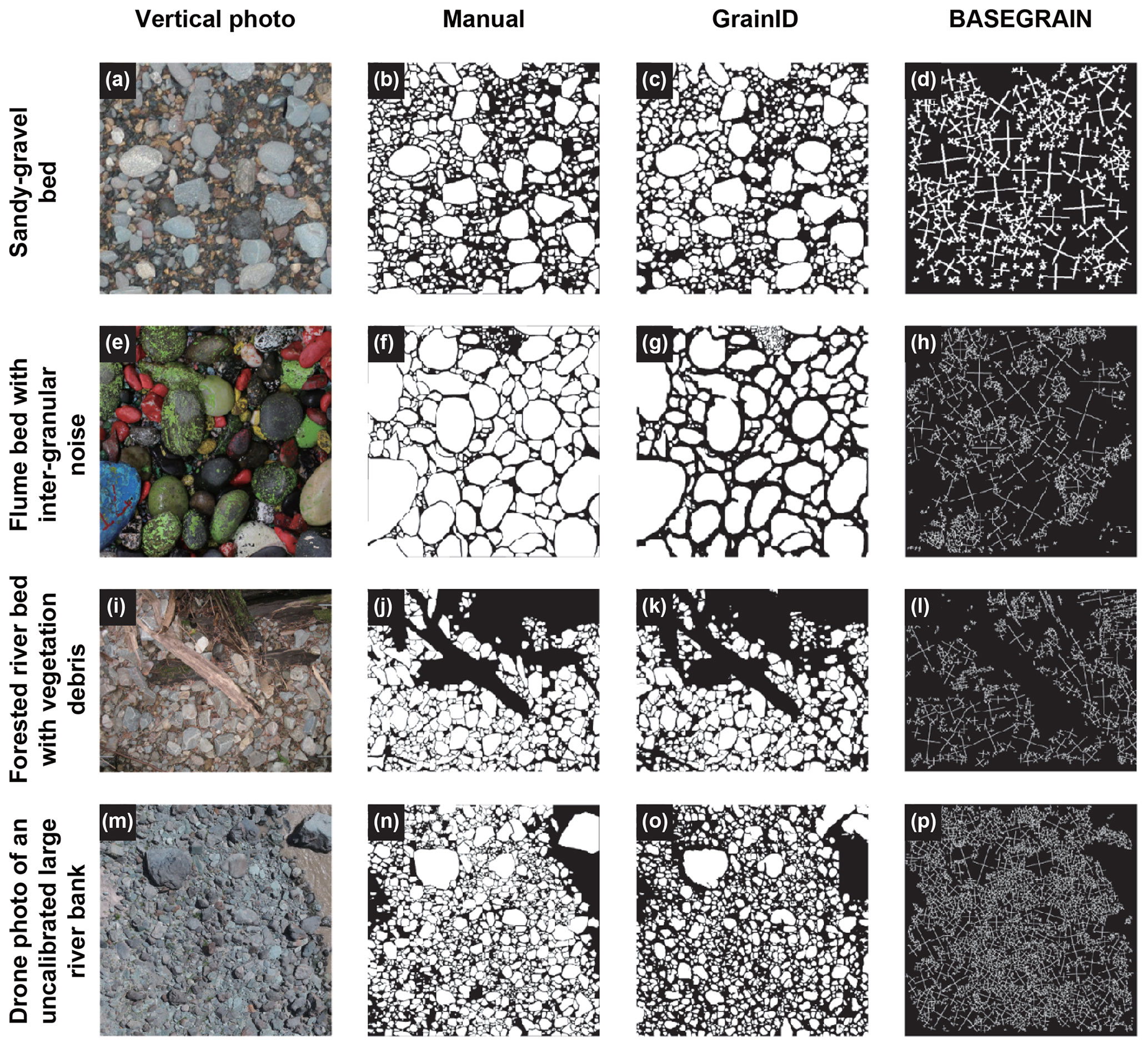
Figure 5Vertical photos and predicting results of manual labeling, GrainID and BASEGRAIN for a variety of environments: (a–d) flume sandy-gravel bed (SAFL dataset); (e–h) flume gravel bed with inter-granular noise (MCHEL dataset); (i–l) location with dense vegetation (Sullivan Creek); and (m–p) drone photo of an uncalibrated large river bank (Yangtze River).
The statistical analysis shows that, for small grains (D5, D16, D50), manual labeling (Err 0.17, 0.10, 0.15) and GrainID (Err 0.16, 0.16, 0.16) significantly outperform BASEGRAIN (Err 0.72, 0.50, 0.30) and Wolman classification methods (Err 0.43, 0.46, 0.26). BASEGRAIN shows much larger variation than the other three methods (Fig. 6a) in terms of Vi,3rd–1st. For large grains (D84, D95), the four methods show similar performance in terms of both Erri,median and Vi,3rd–1st. BASEGRAIN consistently overestimated, while the Wolman method consistently underestimated, grain size for all percentiles. Overall, BASEGRAIN shows the worst performance, while the manual labeling and GrainID methods had comparably great performance in terms of both Erri,median and Vi,3rd–1st.
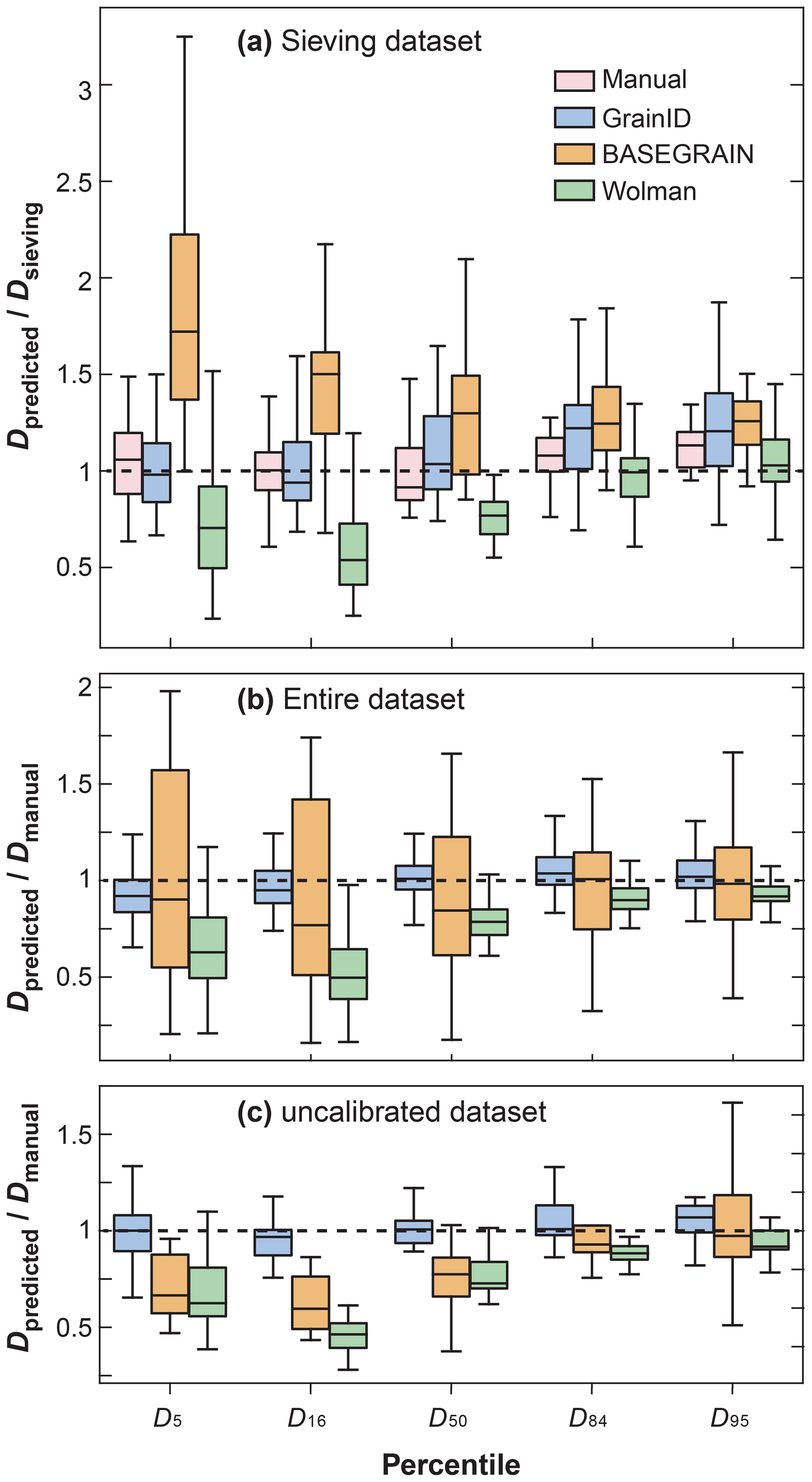
Figure 6Performance comparison for different methods. (a) shown for grain percentiles Di of the manual labeling, GrainID, BASEGRAIN and Wolman methods (referred to as G, B and W methods, respectively) for a flume sandy-gravel bed; (b) shown for Di of G, B and W methods for the entire datasets; and (c) shown for Di of G, B and W methods for uncalibrated rivers with drone photos.
4.2 Comparison of GrainID, BASEGRAIN and Wolman in diverse environments
The entire test dataset (Table 1) was used to evaluate the performance of GrainID, BASEGRAIN and Wolman methods in diverse fluvial environments. In Fig. 5, we present photos (Fig. 5a, e, i, m) and the predictive results of manual labeling (Fig. 5b, f, j, n), GrainID (Fig. 5c, g, k, o) and BASEGRAIN (Fig. 5d, h, l, p). The photos cover a variety of environments in which Fig. 5a is a flume sandy-gravel bed, Fig. 5e shows a flume bed with a wide grain size range and with inter-granular noise, Fig. 5i shows a forested riverbed with vegetation debris (from a small mountain watershed) and Fig. 5m is a drone photo of a large mountain riverbank.
A rough comparison shows that GrainID successfully predicts grains with inter-granular noise (Fig. 5g), while BASEGRAIN falsely recognizes the inter-granular noise as grain boundaries and splits those grains into smaller ones (Fig. 5h). When there is vegetation, GrainID distinguishes grains from large wood elements (Fig. 5k) while vegetation debris is frequently falsely predicted as grains by BASEGRAIN (Fig. 5l). For Fig. 5m, even with water in the image leading to some predictive error due to limited training for this uncalibrated site, GrainID performs well for all grain size groups (Fig. 5o). With BASEGRAIN, the error due to water was partly overcome thanks to human expertise during the parameter tuning process, but the model falsely merges some small grains in the images (Fig. 5p).
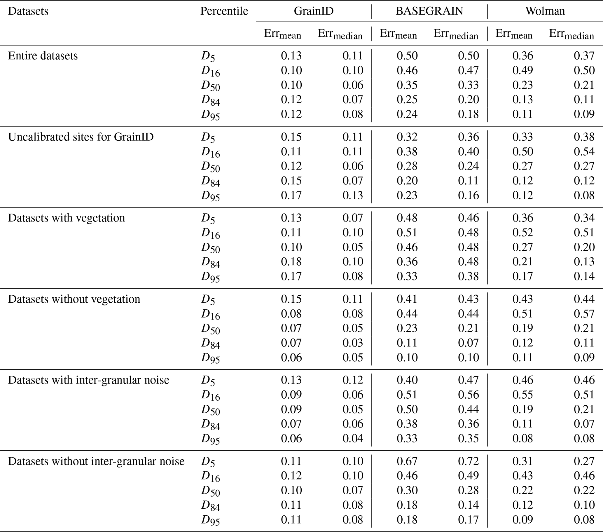
As shown in Table 3, for small grains D5, D16 and D50, GrainID outperforms Wolman and significantly outperforms BASEGRAIN in terms of both Erri,mean and Erri,median. For D84 and D95, GrainID and Wolman show similar performance, while BASEGRAIN shows slightly lower performance than the other two methods. As for prediction variation (Fig. 6b), BASEGRAIN shows significantly larger variation Vi,3rd–1st than the GrainID and Wolman methods for all grain percentiles.
When comparing the change in predictive error versus grain percentiles, Wolman and BASEGRAIN both show larger predictive error for small grains than for large grains. In contrast, GrainID shows similarly consistent performance for all grain percentiles. The results indicate that GrainID is a more accurate and robust grain sizing method (especially for small grains) than the BASEGRAIN and Wolman methods for diverse fluvial environments.
Table 3Median and mean predicting error for different grain sizing methods and for different evaluating datasets with manual labeling as the baseline method.
4.3 Performance of GrainID in uncalibrated sites with airborne photos
To test the predictive ability of GrainID in uncalibrated rivers, 13 drone photos were compiled for sparsely vegetated large rivers (Table 1). As shown in Table 3, GrainID shows slightly lower performance for all grain percentiles than its performance in diverse environments, where most of the evaluated images (53 out of 66) were from calibrated sites. Inversely, BASEGRAIN shows slightly higher performance in these conditions in comparison with its performance in diverse environments, while the predictive error for Wolman in these rivers was similar to its predictive error in diverse environments. Once again, BASEGRAIN and Wolman consistently underestimate grain size (Fig. 6c) and show similar overall performance in terms of Erri,mean and Erri,median. GrainID shows that it outperforms the two methods for all grain percentiles. As for prediction variation (Fig. 6c), GrainID and Wolman show similar variation in terms of Vi,3rd–1st, and BASEGRAIN shows larger variation than the other two methods. The results suggest that GrainID shows better predictive ability than the BASEGRAIN and Wolman methods even in uncalibrated rivers.
4.4 Influence of vegetation and inter-granular noise
The datasets were grouped based on the presence of vegetation and inter-granular noise in the image (Table 1) to evaluate the influence of vegetation and inter-granular noise on the GrainID, BASEGRAIN and Wolman methods. As shown in Table 3, the existence of vegetation and noise have little influence on the performance of GrainID in terms of both Erri,mean and Erri,median for all grain sizes. Conversely, BASEGRAIN shows larger Erri,mean, Erri,median (Table 3) and prediction variation (Fig. 7b) for environments with vegetation and inter-granular noise. For vegetated environments, BASEGRAIN consistently shows larger Erri,median and Vi,3rd–1st for all Di compared with its performance in environments devoid of vegetation (Fig. 7b). For environments without the presence of inter-granular noise, BASEGRAIN consistently overestimates grain size for all Di. Interestingly, however, when there is inter-granular noise, BASEGRAIN consistently underestimates grain size for all Di (Fig. 7b). The performances of Wolman in the four test subsets in this section were similar for all grain percentiles, where there is limited influence from vegetation and inter-granular noise on the performance of the Wolman method (Fig. 7c). Overall, GrainID showed the smallest Erri,median and Vi,3rd–1st, while BASEGRAIN showed the largest Erri,median and Vi,3rd–1s for environments with vegetation and inter-granular noise.
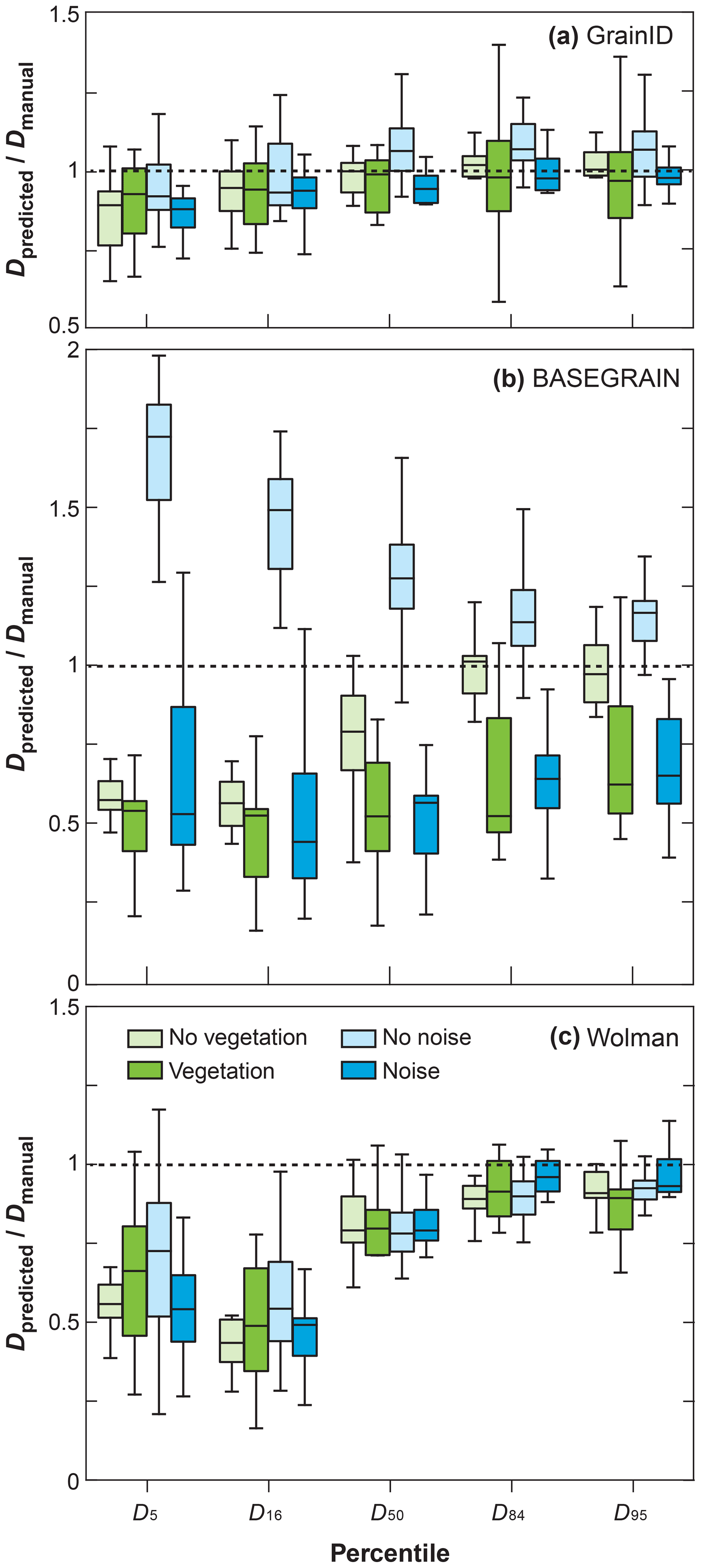
Figure 7Ratio of predicted to baseline grain size value shown for different Di for the (a) GrainID, (b) BASEGRAIN and (c) Wolman methods in environments with and without vegetation and inter-granular noise.
In this section, we first discuss the error sources of different image-based methods based on the results in Sect. 4. Subsequently, we explore the influence of image tile size and image resolution on the predictive ability of GrainID by varying the image tile size and image resolution. Then, the truncation area for the smallest detectable grains is discussed and the model efficiencies of different image-based methods are compared. Finally, the limitations of GrainID and future improvements and studies are discussed.
5.1 Error analysis
The error sources for image-based grain size measurement methods can be divided into five types: (1) the intrinsic error arising from estimating three-dimensional grains with their projection on a two-dimensional image, e.g., the grain vertical axis cannot be detected from an image; (2) errors associated with the image-processing algorithm, e.g., the limitation of the interstice-based algorithm as discussed above; (3) errors associated with suboptimal environments from vegetation, inter-granular noise and suboptimal lighting, and how the boundary of those environmental elements could be falsely detected as grain interstice; (4) errors associated with image tile size and image resolution, and how the smallest detectable grain size is limited by image resolution; and (5) errors associated with grain size distribution, irregular grain shape and photo distortion, and how a wide grain size distribution could lead to larger errors in detecting fine grains. Among the errors above, error type 1 is present for all image-based methods and has been widely discussed in previous literature (Graham et al., 2010), while error type 5 is likely to have little influence on the final prediction results (Sime and Ferguson, 2003; Graham et al., 2005b; Detert and Weitbrecht, 2012). In this section, we will discuss the advantages and disadvantages of the manual labeling, GrainID, BASEGRAIN and Wolman methods (error type 2), and discuss how vegetation, inter-granular noise, image tile size and image resolution influence the model's predictive performance (error types 3 and 4).
Manual labeling, based on the operator's cognitive ability of identifying the grains, is the most robust and reliable method when applied to diverse fluvial environments. The influence of image resolution and image tile size on manual labeling are reduced compared with other models. However, the method is extremely time-consuming and laborious. In addition, the method requires a significant degree of expertise from the operator to correctly identify grains. Labeling errors vary from operator to operator (Fig. 3). Moreover, based on the experience of all five operators in our study, when the operators get tired after hours of labeling work, labeling errors usually increase (especially for fine grains) with operator fatigue. Manual labeling has been widely used as a baseline method for grain detection studies (Sime and Ferguson, 2003; Graham et al., 2005a; Ronneberger et al., 2015) and was used for the training and evaluation of models in this study.
The Wolman pebble count is a semi-automatic grain size measurement method as it requires a manual measurement of at least 100 grains and as a result takes more time to perform in comparison with BASEGRAIN and GrainID. The Wolman method shows consistent predictive ability in diverse environments. Vegetation, inter-granular noise, suboptimal lighting and image resolution have similar influence on the method (Table 3) as seen in manual labeling methods. However, the predictive ability of the Wolman method is sensitive to grain size distribution. The Wolman method shows better predictive ability for large grains (D84, D95) than small grains (D5, D16, D50; Table 3), and the method is limited to material > 8 mm when applied in mountain rivers (Kellerhals and Bray, 1971).
BASEGRAIN, as an automatic grain-detecting model, is less time-consuming than manual labeling and the Wolman method, and is capable of measuring the spatial distribution of grains. The method has been proven in studies to be a reliable grain size measurement method under optimal conditions (no inter-granular noise, no vegetation, and uniform lighting and dryness; Detert and Weitbrecht, 2020). For flume experiments with regular sandy-gravel beds, BASEGRAIN shows good performance for predicting large grains when compared with sieving results (Fig. 5b). However, as shown in Figs. 4 and 5, the model performs poorly in detecting very fine grains (usually less than 50 pixels) even in environments with optimal conditions. In addition, the performance of BASEGRAIN in predicting large grains was highly sensitive to environmental factors such as vegetation and inter-granular noise. BASEGRAIN had poor and inconsistent performance for suboptimal environments (Table 3). The model also evidently overestimates grains without inter-granular noise while underestimating grains with inter-granular noise (Fig. 7b). The reasons are as follows: although BASEGRAIN applied a well-designed algorithm, as introduced in Sect. 3.3, most of the key parameters are calibrated for detecting object interstice (e.g., grayscale threshold filter and bottom-hat filter). When there is vegetation or inter-granular noise in the image, the BASEGRAIN algorithm intrinsically falsely detects the edges of vegetation or inter-granular noise as the edges of grains (Fig. 4). Moreover, as shown in Sect. 4.1, due to the limitations of image resolution, the boundaries of small grains are unclear and detected poorly with simple thresholds. In addition, the model contains 46 adjustable parameters (in which 7 are key parameters) such that BASEGRAIN requires a sophisticated parameter tuning process and a high level of expertise from the operator when applied to suboptimal conditions such as field images.
U-Net, with thousands of neurons and nonlinear activation functions (e.g., sigmoid) in every neuron, is capable of learning the nonlinearity of grain features under diverse environments. Through repeated convolution and pooling on the input images, the machine learning model not only uses grain interstice information but also high-level grain features such as shape, color or texture to make their final predictions (Buscombe, 2020). For field application, the interstice-based algorithms tend to falsely detect environmental elements (e.g., organic debris) and over-split the grains. GrainID is capable of overcoming the influence of environmental elements using grain shape, color or texture features to detect grains. As shown in Sect. 4.2, GrainID evidently outperforms the Wolman and BASEGRAIN models for all grain percentiles for a hold-out testing dataset from diverse environments, and the advantage of GrainID is more significant for small grains than for large grains (Table 3). Moreover, the pooling layer and the drop out training strategy improve the robustness of U-Net. When trained based on tens of thousands of grains, GrainID makes robust predictions for images filmed from a very different environment (uncalibrated rivers) and by a different photography method (airborne photos) compared with the images in the training dataset (Sect. 4.3). In addition, the architecture (Fig. 4) of GrainID overcomes errors arising from image splits (poorer predictive ability of CNN at the border region of an image tile), making it a promising method for large-scale drone surveys. The analysis of drone photos in Sect. 4.3 showed the potential of applying GrainID in large-scale river surveys. Similar to other machine learning methods, the predictive ability of GrainID is highly dependent on the quality of training datasets such as the number and diversity of training images. In Sect. 5.5, we discussed the limitations of GrainID and the issue of lack of training in detail.
5.2 Influence of image tile size and resolution
The model's predictive ability will be influenced by whether the sizes of image tiles are too large (under-split; limited by the GPU memory; Ronneberger et al., 2015) or small (over-split; limited by the size of the largest grain to detect). Based on the forested mountain river and sparsely vegetated large river datasets (Table 1), we explored the influence of image tile size on grain detection ability by varying the image tile size (64 × 64, 128 × 128, 256 × 256, 512 × 512, 768 × 768, 1024 × 1024) while maintaining the raw image resolution. As shown in Fig. 8a, the tile size 64 × 64 yielded positive predictive results for small grains (D5, D16, D50) while it failed to detect larger grain classes (D84, D95). The tile sizes 128 × 128, 256 × 256 and 512 × 512 had a similar predictive accuracy for all grain size percentiles, with 512 × 512 showing the lowest mean predictive error Erri,mean (Eq. 1) for D50 and D84, D95, and the lowest averaged value of Erri,mean for all grain percentiles.
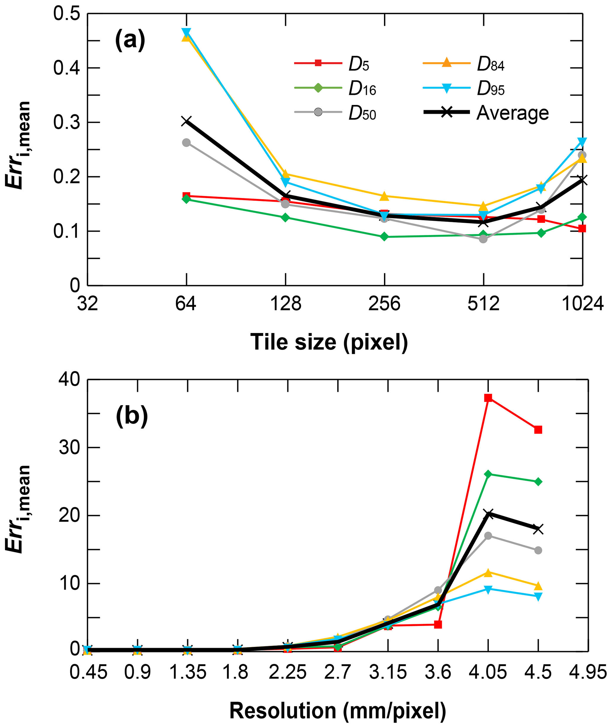
Figure 8Prediction accuracy of different grain percentiles for (a) different image tile size and (b) different image resolution.
Based on the SAFL dataset in which manual sieving data were collected (Table 1), we explored the influence of image resolution on grain size detection by down-sampling the original image resolution of 0.45 up to 4.5 mm pixel−1 and comparing the results of down-sampled images to the sieving results. The down-sampling was done using a simple moving average method of increasing window size from 1 × 1 up to 10 × 10 (the latter controls the spatial resolution; Chen et al., 2020). As shown in Fig. 8b, the predictive error was quite consistent (Erri,mean ∼ 0.10) for resolutions higher than 1.8 mm pixel−1, and increased slowly (from 0.10 to 0.96) for resolutions from 1.8 to 3.15 mm pixel−1 and sharply for resolutions greater than 3.15 mm pixel−1. Erri,mean for small grains were more sensitive to the variable of image resolution than large grains. The analysis showed that for a sandy-gravel bed with D50= 9.5 mm, GrainID can predict all grain percentiles for image resolutions higher than 1.8 mm but failed to predict grain sizes for resolutions lower than 3.15 mm pixel−1.
5.3 Smallest detectable grains
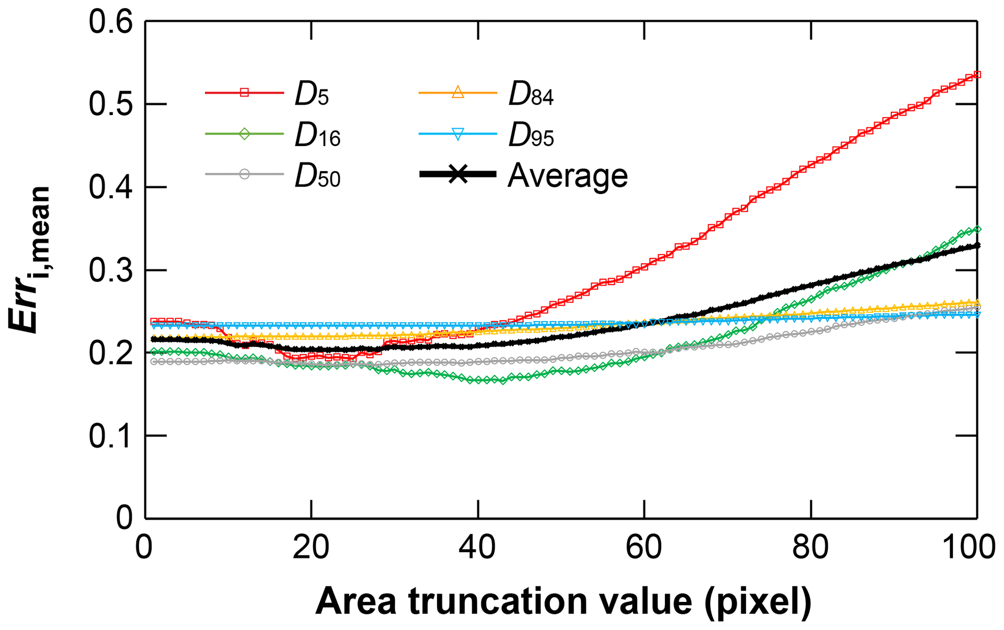
The ability to detect fine grains is limited by image resolution for all image-based grain sizing algorithms. For the smallest detectable grains, Graham et al. (2005a, b) proposed that the measurement error increases sharply for grains with a b axis smaller than 23 pixels, while Detert and Weitbrecht (2012, 2020) adopted a grain area of 23 pixels as the lowest truncation value (the area of smallest detectable grains) to detect grains for BASEGRAIN. Based on the SAFL dataset, we calculated the mean predictive error Erri,mean (Eq. 2) of GrainID in comparison with sieving results for different grain area truncation values (areatrunc). As shown in Fig. 9, Err5,mean (the predictive error of D5) is very sensitive to areatrunc, and Err5,mean slowly decreases from 0.22 to 0.19 for increasing areatrunc from 1 to 18 pixels, had the lowest value of 0.19 for areatrunc between 18–25 pixels and sharply increases to 0.53 for increasing areatrunc from 25 to 100 pixels. The Err16,mean, Err50,mean and Err84,mean (the predictive error of D16, D50 and D84) are less sensitive to areatrunc compared with Err5,mean. However, they have similar three-stage trends to increasing areatrunc, where the error values first decrease with increasing areatrunc (stage 1), then reach a minimum value for an areatrunc period (stage 2), and finally increase for increasing areatrunc (stage 3). In stage 1, the negative correlation between Erri,mean and areatrunc suggests that the smallest detectable grain for GrainID are grains with an area of 18 pixels. In stage 3, the positive correlation between Erri,mean and areatrunc suggests that the areatrunc is too large such that the correct predictions of GrainID were wrongly filtered out. For D95, similar to the previous findings (Graham et al., 2005a), the result shows that Err95,mean are unaffected by areatrunc and remain almost constant for areatrunc from 1 to 100. The analysis above suggests that GrainID performs optimally when the grain area truncation values are equal to 18–25 pixels.
5.4 Model efficiency
To compare the efficiency of the GrainID, BASEGRAIN and Wolman methods, we calculated the time consumed by the three models for predicting images from three typical environments (Table 1): (1) SAFL datasets: 26 images from flume experiments with optimal conditions (Singh et al., 2013); (2) MCHEL datasets: 12 images from flume experiments with sediment with inter-granular noise (Wang et al., 2021); and (3) 15 images from forested mountain rivers (Brayshaw, 2012). For the GrainID, BASEGRAIN and Wolman methods, the rough averaged time of predicting an image was 5, 46 and 962 s for SAFL datasets; 21, 300 and 1000 s for MCHEL datasets; and 22, 600 and 1000 s for the forested rivers datasets (processing time of GrainID depends on GPU; our GPU is GTX 1080Ti).
GrainID needs the shortest predictive time and the Wolman method requires a significantly longer predictive time as the model necessitates the manual labeling of the 100 sampled grains. The predictive time of BASEGRAIN varies in different application environments; BASEGRAIN necessitated much more time for parameter tuning for images from MCHEL and forested rivers than images from SAFL. Images from MCHEL and forested rivers contained significantly different types of images and, as such, to implement BASEGRAIN required an arduous parameter tuning process and a significant level of expertise.
However, it is of value to note that GrainID requires a very long time for cross-validation (∼ 40 h for GTX 1080Ti) and model training (∼ 10 h for GTX 1080Ti), while the BASEGRAIN and Wolman count methods do not need model training. As for model efficiency, the advantage of GrainID lies in that (1) because of the robustness of the model, when the machine learning model is trained based on a sufficiently large dataset, the model can be directly used for a new grain size survey without specifically training for the survey region, and (2) for predicting a large dataset (thousands of images), the advantage of GrainID in predicting is evident, although it needs days of model training.
5.5 Limitations and future work
We tested the robustness and applicability of GrainID by applying it to uncalibrated sites (Sect. 4.3). As our model was trained by more than 65 000 grains under diverse mountain environments, the method was overall robust and outperformed BASEGRAIN and Wolman even for uncalibrated sites. However, the test datasets of uncalibrated sites only included 13 images from four sparsely vegetated mountain rivers. As shown in Fig. 5, due to a lack of training, some large wood debris, unresolved cohesive sands, flow wave and drone marker boards were falsely identified as grains by the program. As such, the application of GrainID to more diverse fluvial environments would require more training datasets from a greater variety of environments. However, preparing training datasets necessitates the use of manual labeling and is therefore time-consuming and laborious. For some images with dense vegetation, even experienced operators may have trouble confidently identifying grains (especially small grains) in the images. Furthermore, as seen in many other object-based methods, the smallest grain size identifiable by GrainID is limited by image resolution and the grain pattern learned by the model is limited by image tile size. How the image tile size and resolution influence the predictive ability of GrainID in a greater variety of environments needs further study. In addition, the present model only identifies the presence of sediment grains in the image in which they were further segmented into pixels either as grains or interstices. We hope that with further development the model can identify vegetation, cohesive sand or other environmental elements so that the model can learn to further distinguish different environmental elements in the image.
With the development in photography and the GPU computation techniques in the future, a GrainID trained on a sufficiently large dataset can be directly used for many grain size surveys without specifically training for the study region. For model efficiency, based on parallel computing, there are already successful real-time image segmentation techniques in commercial use such as the introduction of self-driving cars and robotic perception (Treml et al., 2016; Siam et al., 2018). With more studies on improving the accuracy and efficiency of GrainID, the model could be applied to detect grains in video recordings of flume experiments which is very important for studies on sediment mobility and transport in gravel-bed rivers. In addition, our study indicates that GrainID has the potential to be used towards predicting drone photos. With more studies on applying GrainID to drone images, the model could be applied to watershed-scale surveys to study the changes and spatial distribution of grain sizes in a watershed.
We have proposed an image-based grain detecting model (GrainID) based on convolutional neural networks to detect sediment grain size in diverse fluvial environments. To develop the model, we compiled a dataset of 84 flume and 118 field photos containing more than 115 000 grains covering environments under a wide range of vegetation coverage, grain lithology and lighting conditions.
Tests were performed to compare the predictive ability of GrainID with the performance of manual sieving, manual labeling, BASEGRAIN and Wolman pebble count methods. When using manual sieving as a baseline result, for a flume experiment with a sandy-gravel bed, GrainID (Err 0.16, 0.16, 0.16, 0.23, 0.24 for D5, D16, D50, D84 and D95) showed a predictive ability comparable to that of manual labeling (Err 0.16, 0.10, 0.15, 0.14 and 0.15, respectively) especially for smaller grains. GrainID and manual labeling largely outperform the BASEGRAIN and Wolman methods for smaller grains (D5, D16, D50), but show similar performance with the BASEGRAIN and Wolman methods for larger grains (D84, D95).
For the entire test dataset based on a diverse range of environments, when using manual labeling as the baseline result, GrainID showed the overall best performance and maintained its advantage even in uncalibrated rivers, whereas BASEGRAIN showed the overall worst performance. The test datasets were grouped based on the presence of vegetation and inter-granular noise in the image (Table 1) to evaluate the influence of vegetation and inter-granular noise on the three image-based methods. The results showed that vegetation and inter-granular noise have little influence on the predictive ability of the GrainID and Wolman methods, while BASEGRAIN showed inconsistent predictive ability and larger Erri,median and Vi,3rd–1st in environments with vegetation and inter-granular noise.
We also studied the influence of image tile size and resolution on the predictive ability of GrainID. For the forested mountain rivers and sparsely vegetated large river datasets, GrainID with an image tile size of 512 × 512 pixels had the best performance. For a sandy-gravel bed with D50= 9.5 mm, GrainID performed optimally when the image resolution was higher than 1.8 mm pixel−1 and the grain area truncation values (the area of smallest detectable grains) were equal to 18–25 pixels. The analysis also indicated that GrainID had a higher working efficiency than the BASEGRAIN and Wolman methods in terms of predicting time. The working efficiency of BASEGRAIN is sensitive to environmental conditions, while the average efficiency of GrainID only depended on the size of the input images. Conversely, the average time for the Wolman method analysis was constant for different environments. The error sources of different methods were also discussed, and the limitations and potential of GrainID for detecting sands and vegetation, as well as watershed-scale application, deserve further studies and development.
Datasets and GrainID model code are available at https://doi.org/10.5281/zenodo.5240906 (Chen et al., 2021).
XC prepared the data, established the model, wrote the model code and produced the majority of the paper. MH contributed significantly to the data, the model, the paper and the original idea of the work. XF provided essential help with regard to the data, the original idea of the work and editorial feedback to improve the paper.
The contact author has declared that neither they nor their co-authors have any competing interests.
Publisher’s note: Copernicus Publications remains neutral with regard to jurisdictional claims in published maps and institutional affiliations.
Shawn Chartrand, Tobias Muller and Sam Anderson commented on the early work. Xingyu Chen, Cormac Chui, Lily Liu, Yongpeng Lin and Kai Sun prepared the manual labels. Drew Brayshaw and Carina Helm provided field photos. Jiamei Wang and Xingyu Chen conducted the flume experiment at the University of British Columbia. Cormac Chui commented on the paper. Eric Leinberger prepared the figures. The participation of Xingyu Chen and Xudong Fu was supported by the National Natural Science Foundation of China (NSFC) under grant nos. 91747207, 51525901 and U20A20319. The visit to the University of British Columbia for Xingyu Chen was supported by the China Scholarship Council (file no. 201906210321). This study was funded by the Natural Sciences and Engineering Research Council of Canada (NSERC) Discovery Grants (grant no. RGPIN 249673-12).
This research has been supported by the National Natural Science Foundation of China (grant nos. 91747207, 51525901 and U20A20319), the China Scholarship Council (grant no. 201906210321) and the Natural Sciences and Engineering Research Council of Canada (grant no. RGPIN 249673-12).
This paper was edited by Orencio Duran Vinent and reviewed by Byungho Kang and one anonymous referee.
Adams, J.: Gravel Size Analysis from Photographs, J. Hydr. Eng. Div.-ASCE, 105, 1247–1255, https://doi.org/10.1061/JYCEAJ.0005283, 1979.
An, C., Hassan, M. A., Ferrer-Boix, C., and Fu, X.: Effect of stress history on sediment transport and channel adjustment in graded gravel-bed rivers, Earth Surf. Dynam., 9, 333–350, https://doi.org/10.5194/esurf-9-333-2021, 2021.
Brayshaw, D.: Bankfull and effective discharge in small mountain streams of British Columbia, The University of British Columbia, Vancouver, Canada, 70–71, https://doi.org/10.14288/1.0072555, 2012.
Bunte, K. and Abt, S. R.: Sampling frame for Improving pebble Count Accuracy in Coarse Gravel-bed streams, J. Am. Water Resour., 37, 1001–1014, https://doi.org/10.1111/j.1752-1688.2001.tb05528.x, 2001.
Buscombe, D.: SediNet: a configurable deep learning model for mixed qualitative and quantitative optical granulometry, Earth Surf. Proc. Land., 45, 638–651, https://doi.org/10.1002/esp.4760, 2020.
Buscombe, D., Rubin, D. M., and Warrick, J. A.: A universal approximation of grain size from images of noncohesive sediment, J. Geophys. Res.-Earth, 115, F02015, https://doi.org/10.1029/2009jf001477, 2010.
Carbonneau, P. E., Lane, S. N., and Bergeron, N. E.: Catchment-scale mapping of surface grain size in gravel bed rivers using airborne digital imagery, Water Resour. Res., 40, W07202, https://doi.org/10.1029/2003wr002759, 2004.
Chen, X., Hassan, M. A., An, C., and Fu, X.: Rough Correlations: Meta-Analysis of Roughness Measures in Gravel Bed Rivers, Water Resour. Res., 56, e2020WR027079, https://doi.org/10.1029/2020wr027079, 2020.
Chen, X., Hassan, M., and Fu, X.: CNN for image-based sediment detection applied to a large terrestrial and airborne dataset, Zenodo [data set], https://doi.org/10.5281/zenodo.5240906, 2021.
Church, M., McLean, D., and Wolcott, J. F.: River bed gravels: Sampling and analysis, in: Sediment Transport in Gravel Bed Rivers, edited by: Thorne, C. R., Bathurst, J. C., and Hey, R. D., John Wiley & Sons, New Jersey, USA, 43–79, ISBN 0-471-90914-9, 1987.
Clark, A.: Pillow (PIL Fork) Documentation, readthedocs, https://pillow.readthedocs.io/en/stable/ (last access: 23 April 2022), 2015.
Detert, M. and Weitbrecht, V.: Automatic object detection to analyze the geometry of gravel grains – a free stand-alone tool, in: River Flow 2012, 1st Edition, edited by: Muñoz, R. M., CRC Press, London, UK, 595–600, https://doi.org/10.1201/b13250, 2012.
Detert, M. and Weitbrecht, V.: User guide to gravelometric image analysis by BASEGRAIN, in: Advances in River Sediment Research, 1st Edition, edited by: Fukuoka, S., Nakagawa, H., Sumi, T., and Zhang, H., CRC Press, London, UK, 1789–1795, https://doi.org/10.1201/b15374, 2013.
Detert, M. and Weitbrecht, V.: Determining image-based grain size distribution with suboptimal conditioned photos, in: River Flow 2020, 1st Edition, edited by: Uijttewaal, W., Franca, M. J., Valero, D., Chavarrias, V., Arbós, C. Y., Schielen, R., and Crosato, A., CRC Press, London, UK, 1045–1052, https://doi.org/10.1201/b22619, 2020.
Fujita, I., Muste, M., and Kruger, A.: Large-scale particle image velocimetry for flow analysis in hydraulic engineering applications, J. Hydraul. Res., 36, 397–414, https://doi.org/10.1080/00221689809498626, 1998.
Goodfellow, I., Bengio, Y., and Courville, A.: Deep learning, MIT Press, Cambridge, MA, USA, ISBN 978-0-262-03561-3, 2016.
Graham, D. J., Reid, I., and Rice, S. P.: Automated Sizing of Coarse-Grained Sediments: Image-Processing Procedures, Math. Geol., 37, 1–28, https://doi.org/10.1007/s11004-005-8745-x, 2005a.
Graham, D. J., Rice, S. P., and Reid, I.: A transferable method for the automated grain sizing of river gravels, Water Resour. Res., 41, W07020, https://doi.org/10.1029/2004wr003868, 2005b.
Graham, D. J., Rollet, A.-J., Piégay, H., and Rice, S. P.: Maximizing the accuracy of image-based surface sediment sampling techniques, Water Resour. Res., 46, W02508, https://doi.org/10.1029/2008wr006940, 2010.
Hassan, M. A., Brayshaw, D., Alila, Y., and Andrews, E.: Effective discharge in small formerly glaciated mountain streams of British Columbia: Limitations and implications, Water Resour. Res., 50, 4440–4458, https://doi.org/10.1002/2013wr014529, 2014.
Hassan, M. A., Saletti, M., Zhang, C., Ferrer-Boix, C., Johnson, J. P. L., Müller, T., and Flotow, C.: Co-evolution of coarse grain structuring and bed roughness in response to episodic sediment supply in an experimental aggrading channel, Earth Surf. Proc. Land., 45, 948–961, https://doi.org/10.1002/esp.4788, 2020.
He, K., Zhang, X., Ren, S., and Sun, J.: Deep Residual Learning for Image Recognition, in: Proceedings of the IEEE Conference on Computer Vision and Pattern Recognition (CVPR) 2016, Las Vegas, USA, 27–30 June 2016, 770–778, https://doi.org/10.1109/CVPR.2016.90, 2016.
Helm, C., Hassan, M. A., and Reid, D.: Characterization of morphological units in a small, forested stream using close-range remotely piloted aircraft imagery, Earth Surf. Dynam., 8, 913–929, https://doi.org/10.5194/esurf-8-913-2020, 2020.
Ibbeken, H. and Schleyer, R.: Photo-sieving: A method for grain-size analysis of coarse-grained, unconsolidated bedding surfaces, Earth Surf. Proc. Land., 11, 59–77, https://doi.org/10.1002/esp.3290110108, 1986.
Kellerhals, R. and Bray, D. I.: Sampling procedures for coarse fluvial sediments, J. Hydraul. Division, 97, 1165–1180, https://doi.org/10.1061/JYCEAJ.0003044, 1971.
Klingeman, P. C. and Emmett, W. W.: Gravel bedload transport processes, in: Gravel-bed Rivers. Fluvial Processes, Engineering and Management, edited by: Hey, R. D., Bathurst, J. C., and Thorne, C. R., John Wiley & Sons, New Jersey, USA, 141–179, ISBN 978-047110139, 1982.
Kohl, S. A. A., Romera-Paredes, B., Meyer, C., Fauw, J. D., Ledsam, J. R., Maier-Hein, K. H., Eslami, S. M. A., Rezende, D. J., and Ronneberger, O.: A Probabilistic U-Net for Segmentation of Ambiguous Images, in: 32nd Conference on Neural Information Processing Systems (NeurIPS 2018), Montréal, Canada, 3–8 December 2018, 6965–6975, https://doi.org/10.48550/arXiv.1806.05034, 2018.
Kondolf, G. M.: Assessing Salmonid Spawning Gravel Quality, T. Am. Fish. Soc., 129, 262–281, https://doi.org/10.1577/1548-8659(2000)129<0262:ASSGQ>2.0.CO;2, 2000.
Krizhevsky, A., Sutskever, I., and Hinton, G. E.: Imagenet Classification with Deep Convolutional Neural Networks, in: 26nd Conference on Neural Information Processing Systems (NeurIPS 2012), Lake Tahoe, USA, 3–6 December 2012, 1106–1114, https://doi.org/10.1145/3065386, 2012.
Lang, N., Irniger, A., Rozniak, A., Hunziker, R., Wegner, J. D., and Schindler, K.: GRAINet: mapping grain size distributions in river beds from UAV images with convolutional neural networks, Hydrol. Earth Syst. Sci., 25, 2567–2597, https://doi.org/10.5194/hess-25-2567-2021, 2021.
Leopold, L. B.: An improved method for size distribution of stream Bed Gravel, Water Resour. Res., 6, 1357–1366, https://doi.org/10.1029/WR006i005p01357, 1970.
McEwan, I. K., Sheen, T. M., Cunningham, G. J., and Allen, A. R.: Estimating the size composition of sediment surfaces through image analysis, P. I. Civil Eng.-Water, 142, 189–195, https://doi.org/10.1680/wame.2000.142.4.189, 2000.
Mueller, J. T.: Modelling fluvial responses to episodic sediment supply regimes in mountain streams, The University of British Columbia, Vancouver, Canada, 89–109, https://doi.org/10.14288/1.0377728, 2019.
Oktay, O., Schlemper, J., Folgoc, L. L., Lee, M., Heinrich, M., Misawa, K., Mori, K., McDonagh, S., Hammerla, N. Y., Kainz, B., Glocker, B., and Rueckert, D.: Attention U-Net: Learning Where to Look for the Pancreas, in: 1st Conference on Medical Imaging with Deep Learning (MIDL 2018), Amsterdam, Netherlands, 4–6 July 2018, 1804.03999, https://doi.org/10.48550/arXiv.1804.03999, 2018.
Paszke, A., Gross, S., Massa, F., Lerer, A., Bradbury, J., Chanan G., Killeen, T., Lin, Z., Gimelshein, N., Antiga, L., Desmaison, A., Köpf, A., Yang, E., DeVito, Z., Raison, M., Tejani, A., Chilamkurthy, S., Steiner, B., Fang, L., Bai, J., and Chintala, S.: PyTorch: An Imperative Style, High-Performance Deep Learning Library, in: 32nd Conference on Neural Information Processing Systems (NeurIPS 2019), Vancouver, Canada, 8–14 December 2019, 1–12, https://doi.org/10.48550/arXiv.1912.01703, 2019.
Reid, D. A., Hassan, M. A., Bird, S., Pike, R., and Tschaplinski, P.: Does variable channel morphology lead to dynamic salmon habitat?, Earth Surf. Proc. Land., 45, 295–311, https://doi.org/10.1002/esp.4726, 2020.
Ronneberger, O., Fischer, P., and Brox, T.: U-Net: Convolutional Networks for Biomedical Image Segmentation, in: in: proceedings of the 18th International Conference on Medical Image Computing and Computer-Assisted Intervention, MICCAI 2015, Munich, Germany, 5–9 October 2015, Lecture Notes in Computer Science, 234–241, https://doi.org/10.1007/978-3-319-24574-4_28, 2015.
Rubin, D. M.: A simple autocorrelation algorithm for determining Grain Size from digital images of sediment, J. Sediment. Res., 74, 160–165, https://doi.org/10.1306/052203740160, 2004.
Siam, M., Gamal, M., Abdel-Razek, M., Yogamani, S., Jagersand, M., and Zhang, H.: A Comparative Study of Real-Time Semantic Segmentation for Autonomous Driving, in: 2018 IEEE/CVF Conference on Computer Vision and Pattern Recognition Workshops (CVPRW), Salt Lake City, USA, 18–22 June 2018, https://doi.org/10.1109/cvprw.2018.00101, 2018.
Sime, L. C. and Ferguson, R. I.: Information on grain sizes in gravelbed rivers by automated image analysis, J. Sediment Res., 73, 630–636, https://doi.org/10.1306/112102730630, 2003.
Singh, A., Czuba, J. A., Foufoula-Georgiou, E., Marr, J. D. G., Hill, C., Johnson, S., Ellis, C., Mullin, J., Orr, C. H., Wilcock, P. R., Hondzo, M., and Paola, C.: StreamLab Collaboratory: Experiments, data sets, and research synthesis, Water Resour. Res., 49, 1746–1752, https://doi.org/10.1002/wrcr.20142, 2013.
Tran, L. and Le, M.: Robust U-Net-based Road Lane Markings Detection, in: 2019 International Conference on System Science and Engineering (ICSSE), Dong Hoi, Vietnam, 20–21 July 2019, 62–66, https://doi.org/10.1109/ICSSE.2019.8823532, 2019.
Treml, M., Arjona-Medina, J., Unterthiner, T., Durgesh, R., Friedmann, F., Schuberth, P., Mayr, A., Heusel, M., Hofmarcher, M., Widrich, M., Bodenhofer, U., Nessler, B., and Hochreiter, S.: Speeding up Semantic Segmentation for Autonomous Driving, in: NIPS2016 workshop on Machine Learning for Intelligent Transportation Systems, Barcelona, Spain, 5–10 December 2016, 1–7, https://openreview.net/forum?id=S1uHiFyyg (last access: 23 April 2022), 2016.
Wang, J., Hassan, M. A., Saletti, M., Chen, X., Fu, X., Zhou, H., and Yang, X.: On How Episodic Sediment Supply Influences the Evolution of Channel Morphology, Bedload Transport and Channel Stability in an Experimental Step-Pool Channel, Water Resour. Res., 57, e2020WR029133, https://doi.org/10.1029/2020wr029133, 2021.
Wolman, M. G.: A method of sampling coarse river-bed material, EOS T. Am. Geophys. Union, 35, 951–956, https://doi.org/10.1029/TR035i006p00951, 1954.
Yager, E. M., Venditti, J. G., Smith, H. J., and Schmeeckle, M. W.: The trouble with shear stress, Geomorphology, 323, 41–50, https://doi.org/10.1016/j.geomorph.2018.09.008, 2018.
- Abstract
- Introduction
- Data
- Methods
- Evaluating the predicting ability of image-based grain sizing methods in diverse fluvial environments
- Discussion
- Conclusion
- Code and data availability
- Author contributions
- Competing interests
- Disclaimer
- Acknowledgements
- Financial support
- Review statement
- References