Automated riverbed composition analysis using deep learning on underwater images

The sediment of alluvial riverbeds plays a significant role in river systems both in engineering and natural processes. However, the sediment composition can show high spatial and temporal heterogeneity, even on river-reach scale, making it difficult to representatively sample and assess. Conventional sampling methods are inadequate and time-consuming for effectively capturing the variability of bed surface texture in these situations. In this study, we overcome this issue by adopting an image-based deep-learning (DL) algorithm. The algorithm was trained to recognise the main sediment classes in videos that were taken along cross sections underwater in the Danube. A total of 27 riverbed samples were collected and analysed for validation. The introduced DL-based method is fast, i.e. the videos of 300–400 m long sections can be analysed within minutes with continuous spatial sampling distribution (i.e. the whole riverbed along the path is mapped with images in ca. 0.3–1 m² overlapping windows). The quality of the trained algorithm was evaluated (i) mathematically by dividing the annotated images into test and validation sets and also via (ii) intercomparison with other direct (sieving of physical samples) and indirect sampling methods (wavelet-based image processing of the riverbed images), focusing on the percentages of the detected sediment fractions. For the final evaluation, the sieving analysis of the collected physical samples were considered the ground truth. After correcting for samples affected by bed armouring, comparison of the DL approach with 14 physical samples yielded a mean classification error of 4.5 %. In addition, based upon the visual evaluation of the footage, the spatial trend in the fraction changes was also well captured along the cross sections. Suggestions for performing proper field measurements are also given; furthermore, possibilities for combining the algorithm with other techniques are highlighted, briefly showcasing the multi-purpose nature of underwater videos for hydromorphological assessment.

1 Introduction

The physical composition of a riverbed plays a crucial role in fluvial hydromorphological processes as a sort of boundary condition in the interaction mechanisms between the flow and the solid bed. Within these processes, the grains on the riverbed are responsible for multiple phenomena, such as flow resistance (Vanoni and Hwang, 1967; Zhou et al., 2021), stability of the riverbed (Staudt et al., 2018; Obodovskyi et al., 2020), development of bed armour (Rákóczi, 1987; Ferdowsi et al., 2017), sediment clogging (Rákóczi, 1997; Fetzer et al., 2017), and fish shelter (Scheder et al., 2015). Through these physical processes, the bed material composition has a determining effect on numerous river uses, e.g. the possibility of inland waterway transport (Xiao et al., 2021), the drinking water supply through bank filtration (Cui et al., 2021), or the quality of riverine habitats (Muñoz-Mas et al., 2019). Knowledge of riverbed morphology and sediment composition (sand, gravel, and cobble content) is therefore of major importance in river hydromorphology. In order to gain information about riverbed sediments, in situ field sampling methodologies are implemented.

Traditionally, bed material sampling methods are intrusive (i.e. sediment is physically extracted from the bed for follow-up analysis) and carried out via collecting the sediment grains one by one (areal, grid-by-number, and pebble count methods; e.g. Bunte and Abt, 2001; Guerit et al., 2018) or in a larger amount by a variety of grab samplers (volumetric methods, such as WMO, 1981; Singer, 2008). This is then followed by measuring their sizes individually on site or transporting them to a laboratory for mass-sieving analysis (Fehr, 1987; Diplas, 1988; Bunte and Abt, 2001). These sampling procedures are time- and energy-consuming, especially in large-gravel and mixed-bed rivers, where characteristic grain sizes can strongly vary both in time and space (Wolcott and Church, 1991; USDA, 2007), requiring a dense sampling point allocation. The same goes for critical river reaches, where significant human impact led to severe changes in the morphological state of the rivers (e.g. the upper section of the Hungarian Danube; Török and Baranya, 2017). When assessing bed material composition on a river-reach scale, experts usually try to extrapolate from the samples and describe larger regions of the bed (even several thousand square metres) using data gathered from several dozen points (e.g. USDA, 2007; Haddadchi et al., 2018; Baranya et al., 2018; Sun et al., 2021). Gaining a representative amount of the sediment samples is also a critical issue. For instance, following statistical criteria such as those of Kellerhals and Bray (1971) or Adams (1979), a representative sample should weigh anywhere from tens to hundreds of kilograms. Additionally, physical bed material sampling methods are unable to directly quantify important, hydromorphological features such as roughness or bedforms (Graham et al., 2005). Due to these constraints, surrogate approaches have recently been tested to analyse the riverbed. Examples are introduced in the rest of this section. Unlike the conventional methods, these techniques are non-intrusive and rely on computers and other instrumentation to decrease the need for human intervention and speed up the analyses.

One group of the surrogate approaches includes the acoustic methods, where an acoustic wave source (e.g. an Acoustic Doppler Current Profiler, ADCP) is pointed towards the riverbed from a moving vessel, emitting a signal. The strength and frequency of this signal is measured while it passes through the water column, reflecting back to the receiver from the sediment transported by the river and finally from the riverbed itself. This approach is fast, and larger areas can be covered relatively quickly (Grams et al., 2013). While it has already become widely used for describing sediment movement (i.e. suspended sediment, Guerrero et al., 2016; bedload, Muste et al., 2016; and indirect flow velocity; Shields and Rigby, 2005) and channel shape (Zhang et al., 2008), it has not reached a similar breakthrough for riverbed material analysis. Researchers experimented with the reflecting signal strength (dB) from the riverbed (e.g. Shields, 2010) to establish its relationship with the riverbed material. Their hypothesis was that the absorption (and hence the reflectance) of the acoustic waves reaching the bed correlates with the type of bed sediment. Following initial successes, the method presented several disadvantages and limitations; hence, it could not establish itself as a surrogate method for riverbed material measurements so far. For example, Shields (2010) showed that it was necessary to apply instrument-specific coefficients to convert the signal strength into bed hardness, and these coefficients could only be derived by first validating each instrument using collected sediment samples with corresponding ADCP data. Moreover, the method was sensitive to the bulk density of the sediment and to bedforms. Based on his results and observations, the sediment classification could only extend to differentiate between cohesive (clay, silt) and non-cohesive (sand, gravel) sediment patches, but gravel could not be distinguished strongly from sand as they produced similar backscatter strengths. Buscombe et al. (2014a, b) further elaborated on the topic and successfully developed a better, less limited, decision-tree-based approach. They showed that spectral analysis of the backscatter is much more effective for differentiating the sediment types compared to the statistical analysis used by Shields. With this approach it became possible to classify homogenous sand, gravel, and cobble patches. However, Buscombe et al. (2014a, b) also emphasises that acoustic approaches are not capable of separating the effects of surface roughness from the effects of bedforms; therefore, the selection of an appropriate ensemble averaging window size is of great importance for their introduced method. This size has to be small enough to not include morphological signal, for which the a priori analyses of riverbed elevation profiles is needed at each site. Furthermore, they suggest their method is sensitive to and limited by high concentrations of (especially cohesive) sediment; therefore, its application to heterogeneous riverbeds would require site-specific calibrations. The above-mentioned studies also note that acoustic methods in general inherently do not allow the measurement of individual sediment grains due to their spatial averaging nature. The detected signal strength correlates with the median grain size of the covered area; information about other nominal grain sizes cannot be gained.

Another group of surrogate approaches is the application of photography (Adams, 1979; Ibbekken and Schleyer, 1986) and later computer vision or image-processing techniques. During the last 2 decades, two major subgroups emerged: one uses object and edge detection (by finding abrupt changes in intensity and brightness of the image, segmenting objects from each other; Sime and Ferguson, 2003; Detert and Weitbrecht, 2013), while the other uses analyses the textural properties of the whole image, using autocorrelation and semi-variance methods to define the empirical relationship between the image texture and the grain size of the photographed sediments (Rubin, 2004; Verdú et al., 2005). Both image-processing approaches were very time-consuming and required mostly site-specific manual settings; however, a few transferable and more automated techniques have also been developed recently (e.g. Graham et al., 2005; Buscombe, 2013). Even though there is a continuous improvement in the applied image-based bed sediment analysis methods, there are still major limitations the users face. These limitations include the following problems.

• Most of the studies (all the ones listed above) focus on gravel-bedded rivers, and only a few exceptions can be found in the literature where sand is also accounted for (texture-based methods; e.g. Buscombe, 2013).

• The adaptation environment was typically non-submerged sediment instead of underwater conditions (with a few exceptions, e.g. Rubin et al., 2007; Warrick et al., 2009).

• The computational demand of the image processing is high (e.g. 1–10 min per image; Detert and Weitbrecht, 2013).

• The analysis requires operator expertise (higher than in the case of any conventional method).

• There is an inherent pixel and image resolution limit (Buscombe and Masselink, 2008; Cheng and Liu, 2015; Purinton and Bookhagen, 2019). The finer the sediment, the higher the required resolution of the images will be (higher calculation time). Alternatively, they must be taken from a closer position (smaller area and sample per image).

Nowadays, with the rising popularity of artificial intelligence (AI), several machine learning (ML) techniques have been implemented in image recognition as well. The main approaches of segmentation contra-textural analysis still remain; however, an AI defines the empirical relationship between the object sizes (Igathinathane et al., 2009; Kim et al., 2020) or texture types (Buscombe and Ritchie, 2018) in the images and their real sizes. In the field of river sedimentology a few examples can already be found, where ML (e.g. deep learning, DL) was implemented. For instance, Rozniak et al. (2019) developed an algorithm for gravel-bed rivers, performing textural analysis. With this approach, information is not gained on individual grains (e.g. their individual shape and position) but rather the general grain size distribution (GSD) of the whole image. At certain points of the studied river basins, conventional physical samplings (pebble count) were performed to provide real GSD information. Using this data, the algorithm was trained (with ∼1000 images) to estimate GSD for the rest of the study site based on the images. The method worked for areas where grain diameters were larger than 5 mm and the sediment was well sorted. The developed method showed sensitivity to sand coverage, blurs, reduced illuminations (e.g. shadows), and white pixels. Soloy et al. (2020) presented an algorithm that used object detection on gravel- and cobble-covered beaches to calculate individual grain sizes and shapes. A total of 46 images were used for the model training; however, the number of images was multiplied with data augmentation (rotating, cropping, blurring the images; see Perez and Wang, 2017) to enhance the learning session and increase the input data. The method was able to reach a limited execution speed of a few seconds per square metre and adequately measured the sizes of the gravel. Ren et al. (2020) applied an ensemble bagging-based machine learning (ML) algorithm to estimate GSD along the 70 km long region of Hanford Reach on the Columbia River. Due to its economic importance, a large amount of measurement data has been accumulated for this study site over the years, making it ideal for using ML. By the time of the study, 13 372 scaled images (i.e. their millimetre-to-pixel ratio was known) were taken both underwater and in the dry zones, covering approx. 1 m² each. The distance between the image sampling points was generally between 50 and 70 m. An expert defined the GSD (eight sediment classes) of each image by using a special visual evaluation classification methodology (Delong and Brusven, 1991; Geist et al., 2000). This dataset was fed to a ML algorithm along with their corresponding bathymetric attributes and hydrodynamic properties, simulated with a 2D hydrodynamic model. Following this, it was tested to predict the sediment classes based on the hydrodynamic parameters only. The algorithm performed with a mean accuracy of 53 %. Even though this method was not image-based (only indirectly, via the origin of the GSD data), it highlighted the possibilities of an AI for a predictive model using a high-dimensional dataset. Having such a large dataset of grain size information can be considered exceptional and takes a huge amount of time to gather, even with the visual classification approach they adapted. Moreover, this was still considered spatially sparse information (point-like measurements, 1 m² covered area, and images dozens of metres away from each other). Buscombe (2020) used a set of 400 scaled images to train an AI algorithm on image texture properties using another image-processing method (Barnard et al., 2007) for validation. The algorithm reached a good result for not only gravel but also sand GSD calculation, outperforming an earlier, but promising, texture-based method (wavelet analysis; Buscombe, 2013). In addition, the method required fewer calibration parameters than the wavelet image-processing approach. The study also foresaw the possibility to train an AI that estimates the real sizes of the grains, without knowing the scale of one pixel (mm $/$ pixel ratio) if the training is done properly. The AI might learn unknown relationships between the texture and sizes if it is provided with a wide variety (images of several sediment classes) and scale (mm $/$ pixel ratio) in the dataset (however, it is also prone to learn unwanted biases). Recently, Takechi et al. (2021) further elaborated on the importance of shadow detection and removal using a dataset of 500 pictures for training a texture-based AI with the help of an object-detecting image-processing technique (Basegrain; Detert and Weitbrecht, 2013). The previously presented studies, applying ML and DL techniques, significantly contributed to the development and improvement of surrogate sampling methods, incorporating the great potential of AI. However, there are still several shortcomings to these procedures. Firstly, none of the image-based AI studies used underwater recordings, even though the underwater environment offers completely different challenges. Secondly, the training images were always scaled, i.e. the sizes of the grains could be easily reconstructed, which is again complicated to accomplish in a river. Lastly, they were not adapted for continuous (i.e. spatially dense) measurement but instead focused on a sparse grid-like approach.

The goal of this study is to further investigate the applicability of image processing as a surrogate method and attempt to solve the shortcomings of previous AI-based approaches. Hence, we introduce a riverbed-material-analysing DL algorithm and field measurement methodology and our first set of results. The introduced technique can be used to measure the gravel and sand content of the submerged riverbed surface. It aims to eventually become a practical tool for exploratory mapping, by detecting sedimentation features (e.g. deposition zones of fine sediment, colmation zones, bed armour) and helping decision-making for river sedimentation management. In addition, the long-term hypothesis of the authors includes the creation of an image-based measurement methodology, where underwater videos of the riverbed could serve multiple sediment-related purposes simultaneously. Part of this is the current approach for mapping the riverbed material texture and composition. Others include measuring the surface roughness of the bed (Ermilov et al., 2020) and detecting bedload movement (Ermilov et al., 2022).

Compared to the studies introduced earlier, the main novelty of our study is that both the training and analysed videos are recorded underwater, continuously along cross sections of a large river. Furthermore, the training is unscaled, meaning that the camera–riverbed distance varies while recording the videos without considering image scale. Moreover, compared to the relatively low number of training images in most previous studies, we used a very large dataset (∼15 000) of sediment images for the texture-based AI, containing mostly sand, gravel, cobble, and to a smaller extent bedrock, together with some other, non-sediment-related objects.

2 Methods

2.1 Case studies

The results presented in this study are based on riverbed videos taken during three measurement campaigns in sections of the Danube, Hungary. The first campaign was at Site A, Ercsi settlement (∼ 1606 rkm, river kilometers), where three transects were recorded; the second one was at Site B, Gönyű settlement (∼ 1791 rkm), with two transects; and the third was at Site C, near Göd settlement (∼ 1667 rkm), with three transects (Fig. 1). Each transect was recorded separately (one video per transect); therefore, our dataset included a total of eight videos.

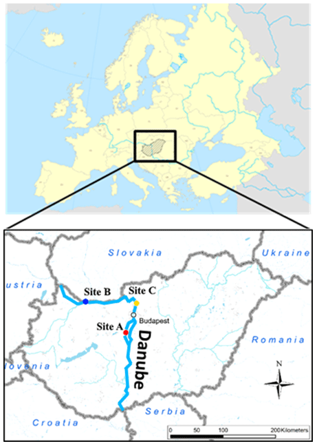
Figure 1 The location of the riverbed videos where the underwater recordings took place. All sites were located in Hungary in central Europe. The surveys were carried out on the Danube, which is Hungary's largest river.

The training of the DL algorithm was done using the video images of Site C and a portion of Site A (test set; see later in Sect. 2.3), while Site B and the rest of the images from Site A served for validation. The measurements were carried out during daytime at a middle-water regime (Q= 1900 m³ s⁻¹) in case of Site A and a low-water regime (Q= 1350 m³ s⁻¹) at Site B and Site C (Q= 700 m³ s⁻¹). This latter site served only for increasing the training image dataset (i.e. conventional samplings were not carried out at the time of recording the videos), and thus we do not go into further details with it for the rest of the study, but the main characteristics are listed in Table 1.

Table 1 Main hydromorphological parameters of the measurement sites. Q_survey is the discharge during the survey, B_survey is the river width during the survey, H_mean,survey is the mean water depth during the survey, S_survey is the riverbed slope during the survey, SSC_survey is the mean suspended sediment concentration during the survey, Q_annual,mean is the annual mean of the discharge at the site, and Q_1 % is for the flooding discharge with a 1 % annual exceedance probability.

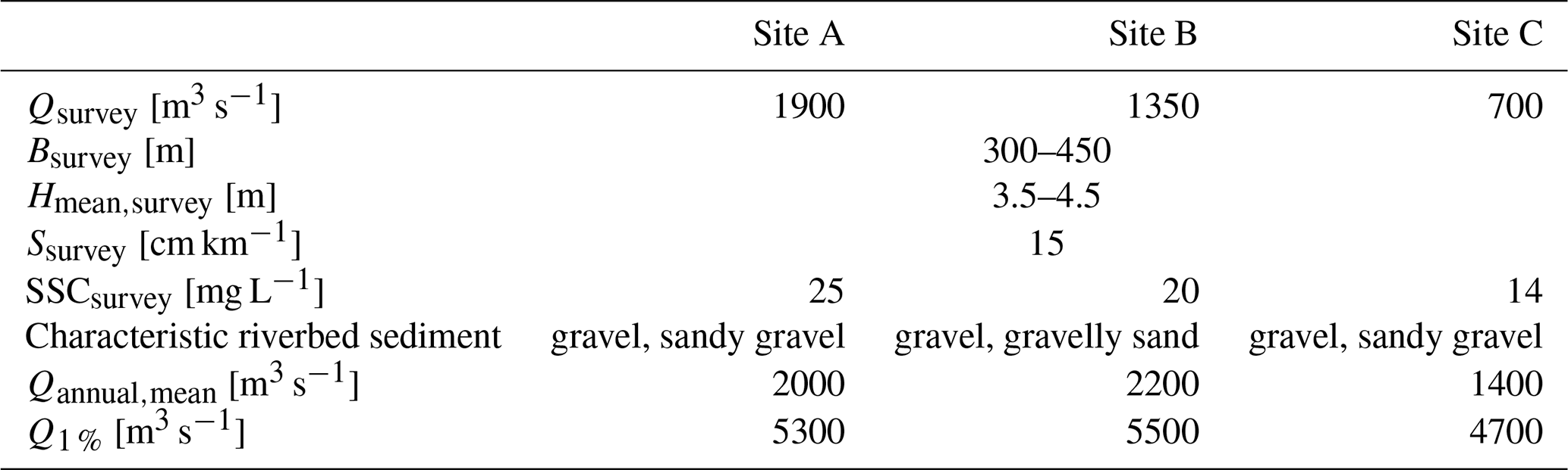
As underwater visibility conditions are influenced by the suspended sediment (SSC_survey – suspended sediment concentration), the characteristics of this sediment transport are also included in Table 1. The highest water depths were around 6–7 m in all cases. At Site A, measurements included mapping of the riverbed with a camera along three separate transects (Fig. 2a). At Site B, two transects were recorded (Fig. 2b).

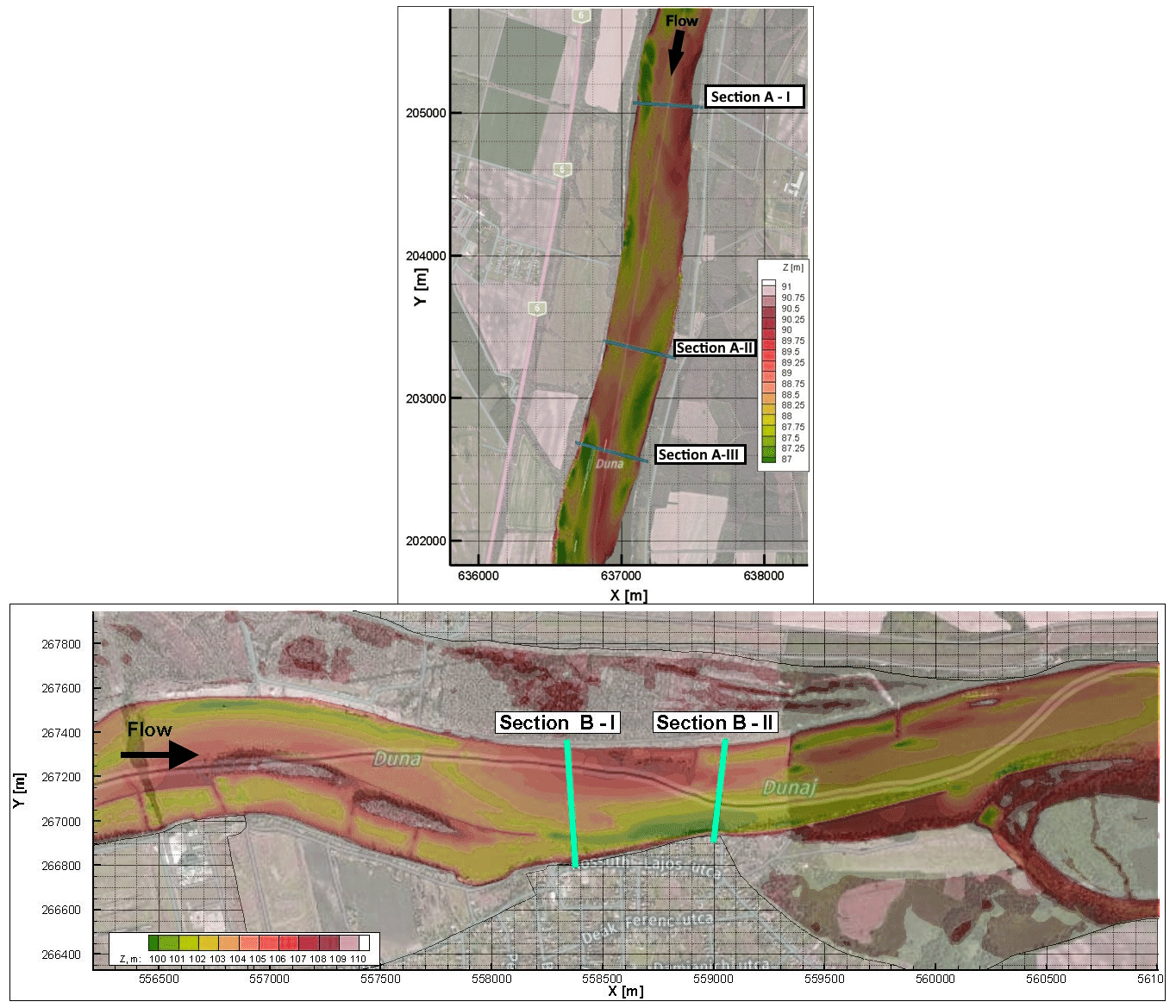
Figure 2 Bathymetry of Site A and Site B. The measurement cross sections are also marked. The vessel moved along these lines from one bank to the other while carrying out ADCP measurement and recording riverbed videos. Physical bed material samples were also collected in certain points of these sections. The x and y coordinates are given in EOV, which refers to the Hungarian Uniform National Projection system (The background aerial images were downloaded from © Google Earth Pro).

2.2 Field data collection

Figure 3 presents a sketch of the measurement process with the equipment and a close-up of the underwater instrumentation. During the field measurements, the camera was attached to a streamlined weight (originally used as an isokinetic suspended sediment sampler) and lowered into the water from the vessel by an electric reel. The camera was positioned perpendicularly to the water and the riverbed in front of the nose of the weight. Next to the camera, two diving lights worked as underwater light sources, focusing into the camera's field of view (FoV). In addition, four laser pointers were also equipped in handmade isolation cases to provide possible scales for secondary measurements. They were also perpendicular to the bottom, projecting their points onto the underwater camera field of view. Their purpose was to ensure a visible scale (mm $/$ pixel ratio) in the video footage for validation. During the measurement procedure, a vessel crossed the river slowly through river transects, while the position of the above detailed equipment was constantly adjusted by the reel. Simultaneously, ADCP and real-time kinematic (RTK) GPS measurement were carried out by the same vessel, providing water depth, riverbed geometry, flow velocity, ship velocity, and position data. Based on this information and by constantly checking the camera's live footage on deck, the camera was lowered or lifted to keep the bed in camera sight and avoid colliding with it. The sufficient camera–riverbed distance depended on the suspended sediment concentration near the bed and the used illumination. The reel was equipped with a register, with its zero adjusted to the water surface. This register was showing the length of cable already released under the water, effectively the rough distance between the water surface and the camera (i.e. the end of the cable). Due to the drag force this distance was not vertical, but this value was continuously compared to the water depth measured by the ADCP. Differencing these two values, an approximation for the camera–riverbed distance was given all the time. The sufficient difference could be established by monitoring the camera footage while lowering the device towards the bed. This value was then to be maintained with smaller corrections during the survey of the given cross section, always supported by observing the camera recording, and adjusting to environmental changes. The vessel's speed was also adjusted based on the video and slowed down if the video was blurry or the camera got too far away from the bed (see later in Sect. 3.3). The measurements required three personnel to (i) drive the vessel; (ii) handle the reel, adjust the equipment position, and monitor the camera footage; and (iii) monitor the ADCP data while communicating with the other personnel (see Fig. 3).

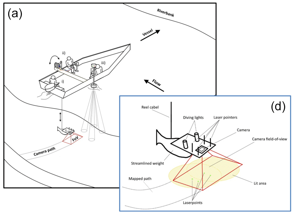
Figure 3 (a) Sketch of the measurement process. The vessel was moving perpendicular to the riverbank along a cross section (i). A reel was used to lower a camera close to the riverbed (ii). Simultaneously, the bed topography and water depth were measured by an ADCP (iii). (b) Close-up sketch of the underwater instrumentation.

The video recordings were made with a GOPRO Hero 7 and a Hero 4 commercial action cameras. Image resolutions were set to 2704×2028 (2.7 K) with 60 frames per second (fps) and 1920×1080 (1080 p) with 48 fps, respectively. Other parameters were left at their default (see GOPRO, 2014, 2018), resulting in slightly different qualities for the produced images between the two cameras. We found that a 0.2–0.45 m s⁻¹ vessel speed with 60 fps recording frequency was ideal to retrieve satisfactory images in a range of 0.4–1.6 m camera–bed distances. This meant approximately 15 min long measurements per transects. Further attention needed to be paid to the reel and its cable during the crossing when the equipment was on the upstream side of the boat. If the flow velocities are relatively high (compared to the total submerged weight of the underwater equipment), the cable can be pressed against the vessel body due to the force from the flow itself, causing the reel cable to jump to the side and leave its guide. This results in the equipment falling to the riverbed and the measurement must be stopped to re-install the cable. For illumination, a diving light with 1500 lumen brightness and 75^∘ beam divergence and one with 1800 lumen and 8^∘ were used. The four lasers for scaling had 450–520 nm (purple and green) wavelength and 1–5 mW nominal power. Power supply was ensured with batteries for all instruments.

At Site A and Site B, conventional bed material (physical) samplings were also carried out by a grabbing (bucket) sampler along the analysed transects. At each cross section, 4–5 samples were taken, with one exception where we had 10. The measured GSDs were used to validate results of the AI algorithm. Separately, a visual evaluation of the videos was also carried out, where a person divided the transects into subsections based on their dominant sediment classes after watching the footage.

2.3 Image analysis: artificial intelligence and the wavelet method

In this study, we built on the former experiences of the authors using Benkő et al. (2020) as a proof of concept, where the developed algorithm was applied for analysing drone videos of a dry riverbed. The same architecture was used in this study, which is based on the widely used Google's DeeplabV3+ Mobilnet, in which many novel and state-of-the-art solutions are implemented (e.g. Atrous Spatial Pyramid Pooling; Chen et al., 2018). The model was implemented with Pytorch, exploiting its handy API and backward compatibility. The main goal was to build a deep neural network model that can recognise and categorise (via semantic segmentation; Chen et al., 2018) at least three main sediment size classes, i.e. sand, gravel and cobble, in the images, while being quickly deployable. The benefit of the introduced method compared to conventional imagery methods lies in the potential of automation and increased speed. If the annotation and training is carried out thoroughly, analysing further videos can run effortlessly, while the computation time can be scaled down either vertically (using stronger GPUs) or horizontally (increasing the number of GPUs if parallel analysis of images is desired). In this study a TESLA K80 24 GB GDDR5 348 bit GPU and an Intel Skylake Intel^® Xeon^® Gold 6144 Processor (24.75 M Cache, 3.50 GHz) CPU with 13 GB RAM were used. In addition, contrary to other novel image-processing approaches in riverine sediment research (Buscombe, 2013; Detert and Weitbrecht, 2013), the deep convolutional neural network is much less limited by image resolution and mm $/$ pixel ratios, because it does not rely on precise pixel count. This is an important advantage to be exploited here, as we perform non-scaled training and measurements with the DL, i.e. camera–bed distance constantly changed, and size references were not used in the images by the DL.

Figure 4 presents the flowchart of our DL-based image-processing methodology. The first step after capturing the videos was to cut them into frames, during which the videos were exploded into sequential images. Our measurement setup proved to be slightly nose heavy. Due to this and the drag force combined, the camera tilted forward during the measurements. As a result, the lower parts of the raw images were sometimes too dark, as the camera was looking over the riverbed and not at the lit part of the bed. In this study, this problem was handled by simply cutting out the lower 25 % of the images as this was the region usually containing the dark, unlit areas. Brightening and sharpening filters were applied on the remaining part of the images to improve their quality. Next, the ones with clearest outlines and best visibility were chosen. This selection process was necessary because this way the delineation process (learning the prominent characteristics of each class) can be executed accurately without the presence of misleading or confusing images, e.g. blurry or dark pictures where the features are hard to recognise. For training purposes, we chose three videos from different sections each being ∼ 15 min long with 60 and 48 fps, resulting in 129 600 frames. In fact, such a large dataset was not needed due to the strong similarity between the consecutive frames. The number of images to be annotated and augmented was therefore decreased to ∼ 2000. We also performed a white balance correction on some of the images to improve visibility, making it even easier to later define the sediment class boundaries. We used an additional algorithm to generate more data, with the so-called simplest colour balance method (Limare et al., 2011). It is a simple but powerful histogram equalisation algorithm that helps to equalise the roughness in pixel distribution.

Figure 4 Flowchart of the applied methodology.

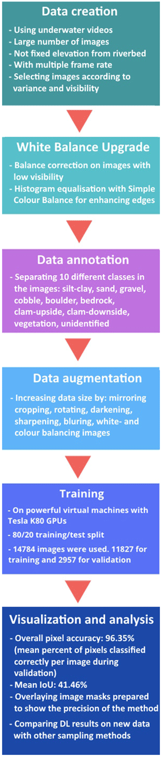
These steps were followed by the annotation, where we distinguished 10 classes: silt-clay, sand, gravel, cobble, boulder (mainly ripraps), bedrock, clam-upside, clam-downside, vegetation, and unidentified (e.g. wreckage). Annotation was carried out by trained personnel, not by the authors, and performed with the help of open-source software called PixelAnnotationTool (Breheret, 2017), which enables the user to colour mask large parts of an image based on colour change derivatives (i.e. colour masking part of the images that belongs to the same class, e.g. purple or red for sand, green for gravel, yellow for cobble). The masks and outlines were drawn manually, together with the so-called watershed annotation. This means that when a line was drawn, the algorithm checked for similar pixels in the vicinity and automatically annotated them with the same class. The annotation was followed by a data augmentation step where beside mirroring, cropping, and rotating the images (to decrease the chance of overfitting), we also convolved them with different filters. These filters added normally distributed noise to the photos to influence the watershed algorithm and applied sharpening, blurring, darkening, and white balance enhancement. Thus, at the data level, we tried to ensure that any changes in water purity, light, and transparency, as well as colour changes, were adequately represented during training. Images were uniformly converted to 960×540 resolution, scaling them down to make them more usable to fit in the GPU's memory. The next step was to convert all the images from red–green–blue (RGB)-based colour to greyscale. This is important because colour images have three channels, meaning that they contain a red, a green, and a blue layer, while greyscale image pixels can only take one value between 0 and 255. With this colour conversion we obtained a 3-fold increase in computational speed. In total, a dataset of 14 784 human-annotated images was prepared (from the ∼ 2000 images of the three training videos). The next step was to separate this dataset into training and validation sets. In this study, we used 80 % of it for training the DL algorithm, while 20 % was withheld and reserved for the validation of the training. It was important to mix the images so that the algorithm selects batches in a pseudorandom manner during training, thus preventing the model from being overfitted. Finally, after several changes in the hyperparameters (i.e. tuning), the evaluation and visualisation of the training results were performed. Tuning is a general task to do when building DL networks, as these hyperparameters determine the structure of the network and the training process itself. Learning rate, for example, describes how fast the network refreshes and updates itself during the training. If this parameter is set too high, the training process finishes quickly, but convergence may not be reached. If it is too low, the process is going to be slow, but it converges. For this reason, nowadays the learning rate decay technique is used, where one starts out with a large learning rate and then slowly reduces it. The technique generally improves optimisation and generalisation of the DL networks (You et al., 2019). In our case, learning rate was initialised to 0.01, with 30 000 iteration steps, and the learning rate was reset after every 5000 iterations with a decay of 0.1. Another important parameter was the batch size, which sets the number of samples fed to the network before it updates itself. Theoretical and empirical evidence suggest that learning rate and batch size are highly important for the generalisation ability of a network (He et al., 2019). In our study, a batch size of 16 was used (other general values in the literature are 32, 64, 128, 256). We used a cross-entropy loss function.

As previously discussed, the training of the deep learning (DL) algorithm proceeded without the application of scaling, obviating the need for the laser equipment. Nevertheless, our original intention was to employ laser pointers to establish a spatial scale for the recorded videos, serving as a supplementary validation measure. Regrettably, the lasers did not operate as initially anticipated, rendering their continuous utilisation during the cross-sectional surveys and the pursuit of transactional scaling and validation unfeasible. Consequently, we shifted our focus to validation at specific physical sampling points, where we could utilise the lasers properly. We adopted a textural image-processing approach to analyse the video images captured at these sampling locations. In this regard, we opted for the previously mentioned transferable wavelet-based signal- and image-processing technique. This method allows for the computation of the image-based grain size distribution from the selected images. The analysis entails examining the greyscale intensity along the pixel rows and columns within the image, treating them as individual signals. This technique utilises the less constrained wavelet transform, instead of the Fourier transform, to decompose these signals. Ultimately, by computing the power spectra and determining the sizes (first in pixel then changing to millimetres using the scale) of the wavelet components (each corresponding to an individual grain), the user can derive the grain size distribution for the given image. Prior to this study, this methodology had demonstrated its efficiency as a non-DL image-processing technique for mixed sediments (Buscombe, 2013, 2020) and had previously been tested by us under underwater conditions as well (Ermilov et al., 2020).

3 Results and discussion

3.1 Evaluation of the training

To evaluate the training process, the 2957 images of the validation set were analysed by the developed DL algorithm, and its results were then compared to their human-annotated counterparts. Figure 5a–d shows results of original images (from the validation set), their ground truth (annotation by the training personnel), and the DL prediction (result of the model). The overlays of the original and the predicted images are also shown for better visualisation. Calculating the overall pixel accuracy (i.e. the percentage of pixels that were correctly classified during validation) returned a satisfactory result with an average 96 % match (over the 2957 validation images, each having 960×540 resolution, adding up to a total of 1 532 908 800 pixels as 100 %). As this parameter in object detection and DL is not a standalone parameter (i.e. it can still be high even if the model performs poorly), the mean IoU (intersection-over-union or Jaccard index) was also assessed, indicating the overlap of ground-truth area and prediction area divided by their union (Rahman and Wang, 2016). This parameter showed a much lower agreement of 41.46 %. Interestingly, there were cases where the trained model gave better result than the annotating personnel. While this highlighted the importance of thorough and precise annotation work, it also showcased that the number of poor annotations was relatively low, meaning that the algorithm could still carry out correct learning processes and later detections, while not being severely affected by the mistake of the training personnel. Figure 5e showcases an example for this: the correct appearance of cobble (yellow) in the prediction, even though the user (ground truth) did not define it during annotation. As a matter of fact, these false errors also decrease the IoU evaluation parameter despite increasing the performance of the DL algorithm over the long term. Hence, this shows that pure mathematical evaluation may not describe the model performance entirely. Considering that others also reported similar experience with DL (Lu et al., 2019) and the fact that 40 % and 50 % are generally accepted IoU threshold values (Yang et al., 2018; Cheng et al., 2018; Padilla et al., 2020), we considered the 41.46 % acceptable, while noting that the annotation and thus the model can further be improved. The general quality of our underwater images may have also played a role in lowering the IoU result.

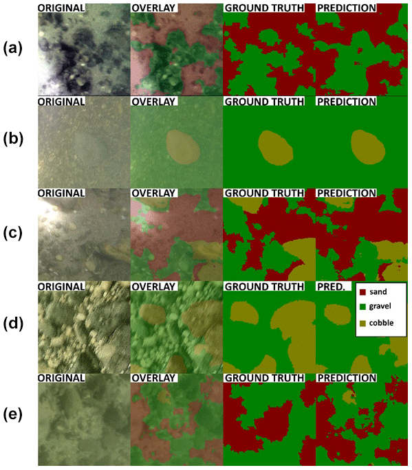
Figure 5 (a–d) Example comparisons of ground-truth (drawn by the annotating personnel, third column) and DL-predicted (result of analysing the raw image by the previously trained DL model, fourth column) results during the validation process. The first column shows raw images, while the second column overlays the result of the DL detection on the raw image for better visual context. (e) Example of training personnel mistake during the annotation (i.e. lack of cobble or yellow annotations in the ground truth) and how the DL performed better by hinting at the presence of the cobble fraction, leading to a false negative result during validation.

One of these quality issues for the DL algorithm was associated with the illumination. Using a diving light with small beam divergence proved counterproductive. The high-intensity focused light occasionally caused overexposed zones (white pixels) in the raw bed image, misleading the DL algorithm and resulting in detection of incorrect classes there (Fig. 6a). In darker zones, where the suspended sediment concentration was higher and at the same time, the effect of camera tilting was not completely removed by preprocessing, the focused light sometimes reflected from the suspended sediment itself and resulted in brighter patches in the images (Fig. 6b). This also caused false positive detections.

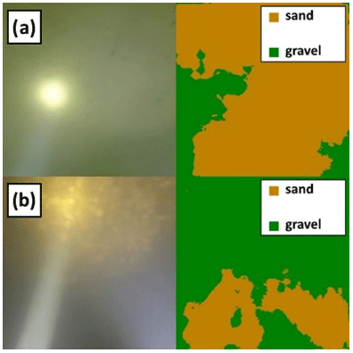
Figure 6 The effect of strong diving light on the DL algorithm. (a) Purely sand-covered zone. (b) Darker zone with higher SSC. The original images are on the left, while the DL detections can be found on the right.

3.2 Comparison of methods

In each masked image, the occurring percentage of the given class (i.e. the percentage of the pixels belonging to that class/colour mask, compared to the total number of pixels in the image) was calculated and used as the fraction percentage in that given sampling point. These sediment classes reconstructed by the DL algorithm were then compared to three alternative results: (i) visual estimation, (ii) GSD resulting from conventional grab sampling, and (iii) wavelet-based image-processing. In the following, results from two cross sections will be highlighted, one from Site A, the video used for the training, and one from Site B, being new for the DL. An averaging window of 15 m was applied on each cross-sectional DL result to smoothen and de-spike the dataset. The interval of physical sample collection in wider rivers can range anywhere between 20 and 200 m within a cross section, depending on the river width and the homogeneity of riverbed composition. The averaging window size was chosen to be somewhat lower than our average applied physical sampling intervals in this study, but still in the same order of magnitude. The scope of the present study did not include further sensitivity analysis of the window size. In the followings, the reader is led through the comparison process via the example of two transects and is given the overall evaluation of the accuracy of the method.

3.2.1 Visual evaluation and physical samples

In Fig. 7a, we depict the vessel's trajectory within Section A-II at Site A. The path is colour coded based on our visual assessment of the riverbed images, with distinct colours representing the prevalent sediment type at each specific location on the riverbed. Additionally, we have marked the positions of physical bed material samples with yellow markers for reference. Figure A1 presents the unprocessed results of the DL detection for each analysed image along Section A-II prior to any moving-average smoothing. It is important to note that our current approach is highly sensitive, occasionally resulting in substantial fluctuations in DL detection between successive, slightly displaced video frames. Owing to this sensitivity and the inherent uncertainty in the coordinates of the underwater photos and their corresponding physical samples, we discourage making direct comparisons by selecting a specific image and its DL detection. Instead, we have implemented a moving-average-based smoothing technique for each raw, cross-sectional DL detection, using a window size of 15 m at each site. These moving averages serve as the basis for comparisons with the physical sampling data and the wavelet method. For the sake of clarity, we have included the raw DL detections of all sampling point images in the Appendices, although these results may not precisely reflect their corresponding moving-average values. In Fig. 7b, we present a comparison between the cross-sectional visual classification and the DL-detected sediment fractions in percentage after applying the moving-average smoothing (i.e. the smoothed version of Appendix Fig. A1). Any noise observed in these results is primarily attributable to abrupt changes in lighting conditions, which can occur either when visual contact with the riverbed is momentarily lost due to sudden bathymetrical changes or as a result of increased suspended sediment concentration. Overall, our DL results exhibit a commendable concordance with human evaluations. For instance, in the vicinity of 100 m from the left bank, between sampling points AII-1 and AII-2, the DL algorithm correctly identifies a peak with approximately 70 % sand and 30 % gravel. Moreover, on either side of this peak, a steep transition to gravel and a decline in sand content are observed, consistent with visual observations, which we have labelled as “sandy gravel” and “gravelly sand”. The DL algorithm also accurately identifies mixed sediment zones on both riverbanks.

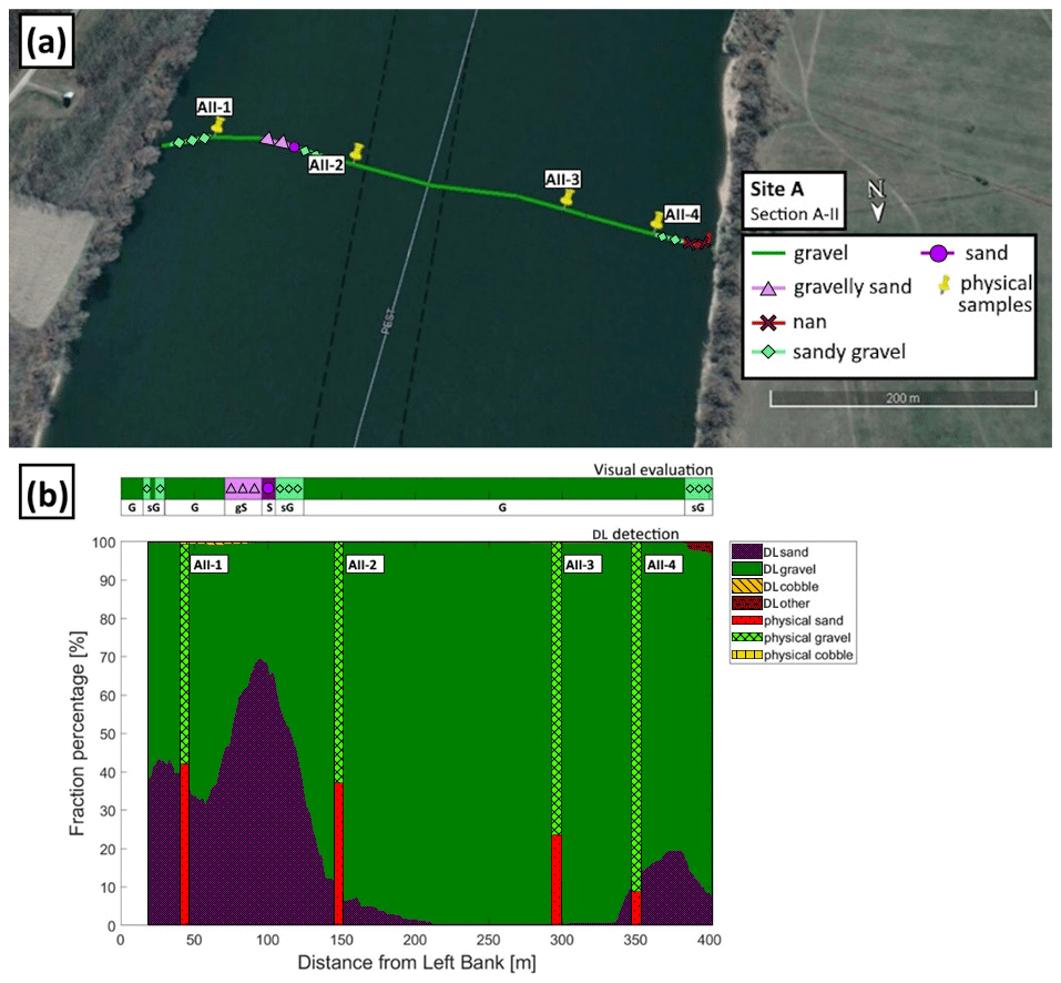
Figure 7 (a) The path of the vessel and camera in Section A-II, Site A. The polyline is coloured based on the sediment features seen during visual evaluation of the video. Yellow markers are the locations of physical bed material samplings (map created with © Google Earth Pro). (b) The visual evaluation of the dominant sediment features in the video (a) compared to sediment fraction percentage recognised by the DL algorithm (b). DL result after applying moving averaging. The visual evaluation included four classes: gravel is shown as G, sandy gravel is shown as sG, gravelly sand is shown as gS, and sand is shown as S). The fractions of the physical samples are shown as verticals.

At site B (Fig. 8a) the river morphology is more complex compared to Site A as a groyne field is located along the left bank (see Fig. 2b). As such, the low-flow regions between the groynes yield the deposition of fine sediments, and much coarser bed composition in the narrowed main stream. As can be seen, the DL algorithm managed to successfully distinguish these zones: the extension of fine sediments in the deposition zone at the left bank were adequately estimated and showed a good match with the visual evaluation for the whole cross section (see Fig. 8b).

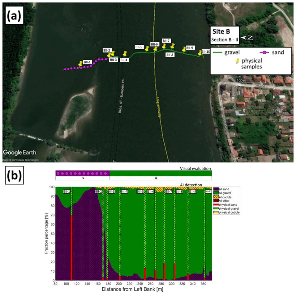
Figure 8 (a) The path of the vessel and camera in Section B-II, Site B. The polyline is coloured based on the sediment seen during visual evaluation of the video. Yellow markers are the locations of physical bed material samplings (map created with © Google Earth Pro). (b) Sediment fraction percentages in Section B-II, recognised by the AI. The visual evaluation included two classes: gravel is shown as G, and sand is shown as S). The fractions of the physical samples are shown as verticals.

Results of the other measurements can be found in the Appendix Figs. C2, D2, and E2. These figrues show that the trend of riverbed composition from the visual evaluation is well captured by the DL algorithm in the other cross sections of the study as well.

Next, the physically measured and DL-detected relative proportion of sand, gravel, and cobble fractions were compared in each of the 27 sampling points. First, however, outliers or incomparable data had to be identified. In our case, this meant the separation of sampling points where the differences between the results of the two methods were independent from the efficiency and performance of the DL algorithm. This selection was carried out after analysing the grain size distribution curves of the weight-sieved physical samples (Fig. F1) and the riverbed images around the sampling points (Figs. A3, B1, C4, D4, E4). Based on our findings, the outliers have been identified and separated into Outlier Type A and Outlier Type B categories. The first category includes the sampling points where the GSD curves showcased bimodal (gap-graded) distributions. This type of riverbed sediment distribution is a typical sign of riverbed armouring (Rákóczi, 1987; Marion and Fraccarollo, 1997), where a coarse surface layer protects the underlying finer subsurface substrate (e.g. Wilcock, 2005). While the camera only sees the upper layer, the bucket sampler can penetrate the surface and gather samples from the subsurface as well. As a result, the two methods cannot be compared solely based on the surface distribution. In Fig. A2, supportive images of bed armouring are provided, taken during our surveys in the upper section of the Hungarian Danube. Out of the 27 sampling points, 11 were affected by armouring and categorised as Outlier Type A. The category of Outlier Type B consisted of points from the opposite case, i.e. where the riverbed image contained fine sediment, but the physical samples did not. In these cases, a relatively thin layer of fine sediment covered the underlying gravel particles. Two sampling points were categorised as Outlier Type B, both of which were near the borderline between a deposition zone behind a groyne and the gravel-bedded main channel. In these cases, the bucket sampler probably either stirred up the deposited fine sediment and washed it down during its lifting or was dragged through purely gravel-bedded patch during sampling, as the surface composition was rapidly changing on this previously mentioned borderline. It is important to highlight that the analysis of physical samples involves measuring and weighing various sediment size classes, leading to weight distribution. In contrast, imaging methods offer surface distributions, and as a consequence the presence of a thin layer of fine sediments on the surface can significantly skew the resulting composition (Bunte and Abt, 2001; Sime and Ferguson, 2003; Rubin et al., 2007).

Overall, the DL-based classification agreed well within the comparable sampling points, with an average error of 4.5 % (Fig. 9). It can be seen that even though in outlier points AII-1 and AI-3 the DL algorithm coincidentally gave good match with the sieving analysis, in the rest of the outlier points the DL- and physical-based results systematically differ from each other, supporting our outlier selection methodology. Table 2 summarizes and showcases the final number of samples in each category after the selection process.

Table 2 After evaluating the results of the sieving analyses and riverbed surface images, out of the 27 sampling points, 14 were defined as comparable between the applied sampling methods. A total of 11 points were categorised as Outlier Type A because their GSD curves were bimodal. Only two points were defined as Outlier Type B, since their images showed the presence of fine sediment, while the sieve analyses did not.

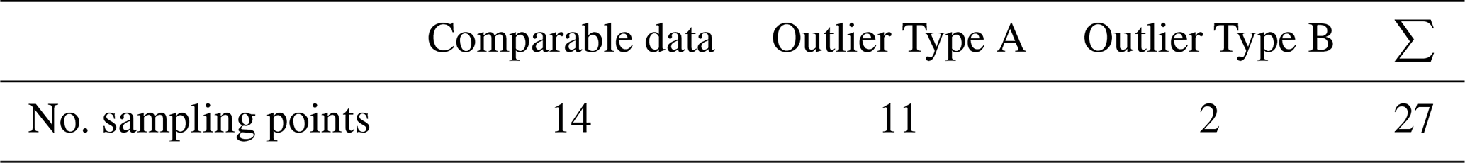
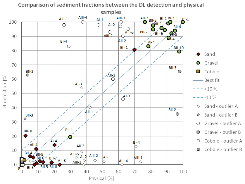
Figure 9 Comparison of relative sediment fractions between the DL detection and physical samples. The three main sediment types (sand, gravel, and cobble) are marked with different colours and symbols. The name of the sampling points where the given relative proportion was measured was detected is also written for gravel and sand (cobble was negligible). The proportions of outlier sampling points are marked with white and grey, while the symbol represents the sediment type, respectively. The comparable points have their proportions with green (gravel) and red (sand) symbols.

3.2.2 Wavelet analysis

Regarding the wavelet-analysis-based imaging technique, it is evident that there is a slight overall overestimation of coarse particles, and the accurate reconstruction of sand classes is not achieved. This observation aligns with our earlier field experiences reported in Ermilov et al. (2020), where we highlighted the wavelet technique's pronounced sensitivity to image resolution. We demonstrated that to successfully detect a grain, its diameter must be at least 3 times larger than a pixel. In the subsequent analysis, we compare the sediment proportions determined by the wavelet-based method to those obtained earlier through DL and physical-based approaches, presenting the results in bar plots (Figs. 10, 11). For instance, when the camera was positioned closer to the riverbed at sampling points AII-1 and AII-4, resulting in a more favourable mm $/$ pixel ratio, the wavelet algorithm was able to detect coarse sand accurately. However, it struggled to identify finer sand, leading to lower sand percentage estimates (Fig. 10). In other sampling points where sand particles were below the resolution limit, the wavelet method consistently identified the presence of cobbles instead (Fig. 10), a distinction not made by the other two methods. This pattern broadly characterises the wavelet method's performance during our study. For illustrative purposes, we provide an example highlighting the differences in the capabilities of these two methods in Fig. 12. While both methods detect the presence of two major sediment categories, the wavelet technique interprets the information as a mixture of gravel and cobbles, whereas the DL algorithm recognises the presence of sand coverage and gravel particles.

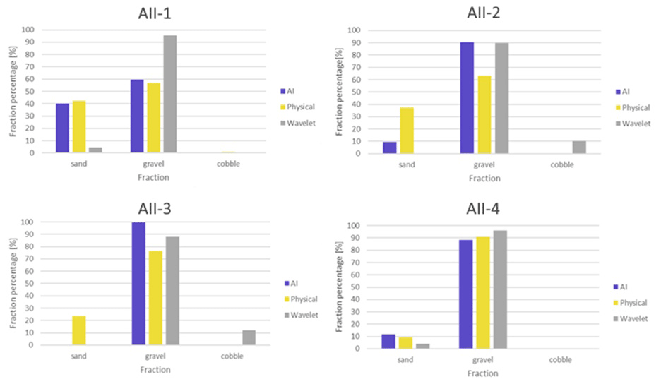
Figure 10 Comparison of relative sediment fraction proportions (%) at the sampling locations from the moving-averaged DL detection, conventional sieving, and wavelet-based image-processing method. Section A-II.

Figure 11 Comparison of relative sediment fraction proportions (%) at the sampling locations from the moving-averaged DL detection, conventional sieving, and wavelet-based image-processing method. Section B-II.

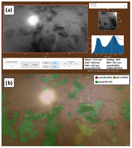
Figure 12 (a) Wavelet analysis result of the underwater image in BII-2. Section B-II. (b) DL detection result of the same image.

Overall, the comparison between the two image-based methods showed greater discrepancies (Fig. 13) due to the limitations of the wavelet approach discussed earlier. The same sampling points as earlier were labelled as outliers. As can be seen, the wavelet significantly differed in the points where the physical samples and DL detections matched (green data points), due to its excessive and false cobble detections. However, it showed good agreement with the DL in most of the outlier points, supporting the earlier observation that the surface in those points was solely composed of gravel and that the finer fractions of the physical samples must have come from the subsurface. Hence, the outlier selection process was well grounded.

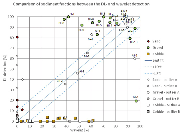
Figure 13 Comparison of sediment fractions between the DL detection and the wavelet approach for the selected sampling points. The three main sediment types (sand, gravel, and cobble) are marked with different colours (red, green, and yellow) and symbols (diamonds, circles, and squares), respectively. The name of the sampling points where the given relative proportion was measured or detected is also written for gravel. The proportions of outlier sampling points are marked with white or grey, while the symbol represents the sediment type. The comparable points have their proportions with green (gravel) and red (sand) symbols.

Based on the results presented in this study, it could be established that the DL algorithm managed to recognise the main features of the riverbed material composition from underwater videos with satisfactory accuracy in the comparable sampling points (based on the sieving analysis of physical samples) and along cross sections (based on the visual evaluation). The method showed good potential for mapping heterogenous riverbeds along river cross sections. Furthermore, the wavelet proved to be a limited comparison tool with the introduced field measurement methodology, as this latter method did not provide it with the sufficient resolution most of the time.

3.3 Implementation challenges

The power supply for the entire imaging infrastructure, including the camera, diving lights, and lasers, relied on batteries. However, due to the lower temperatures at the river bottom, the battery depletion rate was significantly accelerated compared to typical conditions. To address this issue, we explored the option of a direct power supply from the motorboat. Ensuring the camera's optimal positioning posed challenges as well. Proximity to the riverbed risked damage to the equipment, while excessive camera–bed distances compromised image quality. To maintain a clear view of the riverbed while avoiding blurry images, we utilised real-time ADCP water depth data to adjust the camera's position, while simultaneously optimising the boat's velocity. Increasing the recording frequency and reducing exposure time emerged as potential solutions to mitigate this limitation. Lower vessel velocities were not feasible, as they would have caused the vessel to drift out of the desired section. Alternatively, moving along longitudinal (streamline) paths rather than transects may present the opportunity for slower vessel speeds, potentially resulting in higher-quality images in the future. However, the conventional approach for river bathymetry surveys typically involves transversal paths due to lower spatial variations along streamlines compared to the transverse direction (Benjankar et al., 2015; Kinsman, 2015). Therefore, implementing longitudinal paths may require a denser network to obtain sufficient data, thus increasing time demands. Hence, careful consideration of path selection and interpolation methods becomes critical for this alternative approach. Another challenge pertained to the impact of drag force on the measurement setup. Although the main body had a streamlined design, the addition of other tools disrupted the setup's geometry. Additionally, we encountered a slight imbalance in weight distribution. Long-term solutions could involve constructing a streamlined container (e.g. a 3D-printed body or a body resembling uncrewed underwater vehicles) with designated slots for each device and improving weight distribution. Furthermore, we hypothesised that using lasers (as originally planned in this study) during measurements could assist in orthorectifying the images, leveraging the known structure and positioning of laser points' projections when the setup is perpendicular to the riverbed. This could reduce the impact of occasional tilting, which may affect size analysis if scaling is included. In our specific case, we demonstrated that the wavelet method had inherent limitations (e.g. image resolution limits) when applied within our methodology, issues not attributable to camera tilting, as these would have had a significantly lower error magnitude.

As for the training of the DL algorithm with the underwater images, the illumination is indeed a more crucial aspect compared to normal imagery methods. In many cases only the centre areas of the images were clearly visible, whereas the remaining parts were rather dark and shady. Determining the boundaries between distinct sediment classes for these images was challenging even for experienced eyes. This quality issue generated incorrect annotations at first. To overcome this issue, manually varying the white balance and thus enhancing the visibility of the sediment could improve the results of the training. It is known that when DL methods are used, most of the problems arise from the data side (Yu et al., 2007), whereas issues related to the applied algorithms and hardware are rare. This is because data are more important from an accuracy perspective than the actual technical infrastructure (Chen et al., 2020). The time demand of image annotation (data preparation) is relatively high; i.e. a trained person could analyse roughly 10 images per hour. On the other hand, as introduced earlier, a great advantage of using DL is the capability of improving the quality of training itself, often yielding better agreement with reality compared to the manual annotation. Similar results have been reported by Lu et al. (2019). At the same time, this proves that there is no need for very precise manual training with the introduced approach, thus a fast and effective training process can eventually be achieved.

The validation of the DL algorithm is far from straightforward. In this study, four approaches were adopted: a mathematical approach and comparison with three other measurement methods. The mathematical approach was based on calculating pixel accuracy and the intersection-over-union parameter, as is usually done in case of DL methods to describe their efficiency (e.g. Rahman and Wang, 2016). However, the DL model in some cases over-performed and provided more accurate results for the sediment composition than the human annotator did. This meant the calculated difference between the annotated validation images and their responding DL-generated result did not solely originate from the underperformance of the DL model but from human error as well. Consequently, using only the mathematical evaluation in this study could not adequately describe the model performance. Hence, the results were compared to those of three other methods: (i) visual evaluation of the image series, (ii) a wavelet-based image-processing method (using the method of Buscombe, 2013), and (iii) riverbed composition data from physical samples. Considering the features of the applied methods, the first one, i.e. the visual observation, is expected to be the most suitable for the model validation. Indeed, when assessing the bed surface composition by eye, the same patterns are sought, i.e. both methods focus on the uppermost sediment layer. On the other hand, the physical sampling procedure inherently represents subsurface sediment layers, leading to different grain size distributions in many cases. For instance, as shown earlier, if bed armour develops in the riverbed and the sampler breaks up this layer, the resulting sample can contain the finer particles from the subsurface. On the contrary, in zones where a fine-sediment layer is deposited on coarse grains, i.e. a sand layer on the top of a gravel bed, the physical samples represent the coarse material too; moreover, considering that the sieving provides weight distribution, this sort of bias will even enhance the proportion of the coarse particles. Attempts were made to involve a third, wavelet-based method for model validation. However, this method failed when finer particles, i.e. sand, characterised the bed. This is an inherent limitation of these type of methods, as discussed earlier, i.e. when the pixel size is simply not fine enough to reconstruct the small grain diameters in the range below fine gravel. Lastly, the most comparable sample points were selected to quantify the performance of the DL. Holding the sieved physical samples as ground truth, the DL algorithm showed promising results. The average error (difference) between DL-detected and physically measured relative sediment fraction portion percentages was 4.5 %. Furthermore, the DL algorithm successfully detected the trend of changing bed composition along complete river cross sections.

As previously shown, the ML and DL models can learn unknown relationships in datasets but can also learn unwanted biases as well. With our current dataset, these biases would be the darker tones of visible grain texture and the lack of larger grain sizes. This way our model in its current state is only effectively applicable in the chosen study site until the dataset is expanded with additional images from other rivers or regions. However, the purpose of the study was to introduce the methodology itself and its potential in general and not to create a universal algorithm.

3.4 Novelty and future work

The introduced image-based DL algorithm offers novel features in the field of sedimentation engineering. First, to the authors' knowledge, underwater images of the bed of a large river have not yet been analysed by AI. Second, the herein-introduced method enables extensive mapping of the riverbed composition, in contrast to most of the earlier approaches, where only several points or shorter sections were assessed with imagery methods. Third, the method is much faster compared to conventional samplings or non-DL-based image-processing techniques. The field survey of a 400 m long transect took ∼ 15 min, while the DL analysis took 4 min (approx. seven images per second). The speed range of 0.2–0.45 m s⁻¹ of the measurement vessel and the 15 min per transect setting complies with the operating protocol of general ADCP surveys on rivers (e.g. RD Instruments, 1999; Simpson, 2002; Mueller et al., 2009). Hence, the developed image-based measurement can be carried out together with the conventional boat-mounted ADCP measurements, further highlighting its time efficiency. Therefore, the method offers an alternative approach for assessing riverbed material on the go in underwater circumstances. As an extensive and quick mapping tool, it can support other types of bed material samplings in choosing the sampling locations and their optimal number. Furthermore, it can be used for quickly detecting areas of sedimentation and their extent, as we showed in Sect. 3.2. (e.g. Fig. 12b). This way, it can support decision-making regarding the maintenance of the channel or the bank-infiltrated drinking water production (detecting colmation zones). Fourth, a novel approach was used for the imaging and model training. As the camera–bed distance was constantly changing, the mm $/$ pixel ratio also varied. Hence, no scale was defined for the algorithm beforehand. As we discussed in Sect. 1., earlier DL methods for sediment analysis (e.g. Soloy et al., 2020) all applied fixed camera heights and/or provided scaling for the AI. Furthermore, these studies were based on airborne measurements, mapping the dry zone of the rivers. In an underwater environment, it is extremely challenging to keep a fixed, constant camera height due to the spatially varying riverbed elevations. By avoiding the need for a scale, our method is faster and simpler to use. As a drawback, our method does not reconstruct detailed grain size distributions but instead measures the relative portions of the main sediment classes: sand, gravel, and cobble. In short, this study showcased a fast bed material mapping tool with a much denser spatial resolution than the conventional methods that saves significant resources.

Originally, in addition to the three classes of main sediment types introduced in the study, others were also defined during annotation (e.g. bedrock, clams), but due to class imbalance (i.e. dominance of the three sediment classes) these were not discriminated successfully. In the future, improving the method through transfer learning (Zamir et al., 2018) using a broader dataset and involving other sediment types will be considered. Another option for developing the method is to counter imbalance with the use of so-called weighted cross entropy (see Lu et al., 2019) on the current dataset, which will also be investigated.

Since the introduced method offers a quick way to provide extensive, spatially dense bed material information of its composition, it can be used to boost the training dataset of predictive, ensemble bagging-based machine learning techniques (e.g. Ren et al., 2020) and improve their accuracy. Furthermore, the method can support the implementation of other imaging techniques. For instance, using one of the training videos of this study the authors managed to reconstruct the grain-scale 3D model of a riverbed section with the structure-from-motion technique (Ermilov et al., 2020), enabling the quantitative estimation of surface roughness. Underwater field cameras can also be used for monitoring and estimating bedload transport rate (Ermilov et al., 2022) by adapting large-scale particle image velocimetry and the statistical background model approach. This latter videography technique may also be used with moving cameras (e.g. Hayman and Eklundh, 2003), which enables its adaptation into our method, e.g. by detecting bedload movement in the cross section.

The statistical representativity of the introduced method as a surface sampling technique also needs to be addressed in future work. Following and building upon the experience of conventional, surface sampling procedures (e.g. grid sampling; Diplas, 1988) may prove to be beneficial when they provided the exact number of gravel particles needed to be included (Wolman, 1954) to satisfy the representativity criteria. In addition, using edge and blob detection would enable the calculation and comparison of the number of gravel particles in the images to this value. Furthermore, we intend to apply two cameras with overlapping FoVs for increasing the covered area (and the representativity) during surveys. This would also improve the accuracy of the structure-from-motion technique mentioned earlier.

4 Conclusion

We introduced a novel, AI-based method for riverbed sediment analysis. The method uses underwater images to reconstruct spatial variations in sediment grain sizes. Trained and validated with ∼ 15 000 underwater images collected in a section of the Danube in Hungary, we showed that the method can map the riverbed along the vessel's route at a high spatial density of approximately 60–100 overlapping sample images per metre. The method does not require a scale and thus allows the distance between the camera and the riverbed to vary. In contrast with conventional point samples of riverbed substrate, our method provides spatially continuous data that can be further enhanced (e.g. by interpolation) to 2D maps. The method can be applied in studies where dense information about riverbed composition is required, such as riverine habitat studies, computational hydro- and morphodynamic models, or analyses of river restoration measures.

Appendix A: Site A – Section A-II

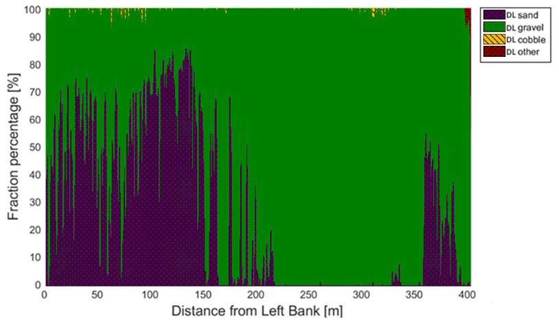
Figure A1 The sediment fraction percentage results of every image, analysed by the DL algorithm along Section A-II. While the trends are apparent, the sensitivity of the method at its current state can be observed. DL result before applying moving averaging.

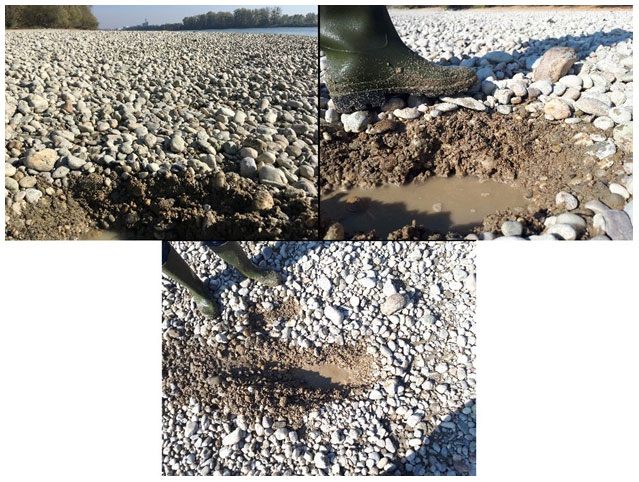
Figure A2 Images of bed armouring taken during our surveys in the upper section of the Hungarian Danube. We broke the surface armour to showcase the presence of the underlying finer fractions.

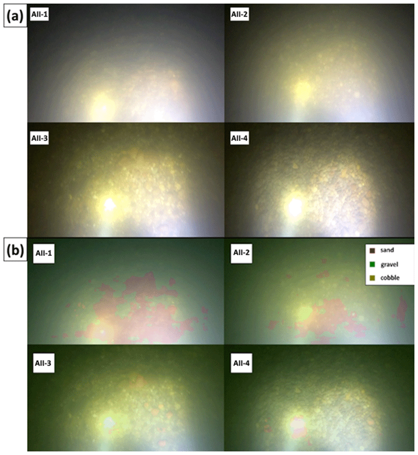
Figure A3 (a) Riverbed video images at the sampling points in Section A-II. (b) Riverbed video images overlapped with their raw, DL detection result at the sampling points in Section A-II.

Appendix B: Site B – Section B-II

Figure B1 Riverbed video images at the sampling points in Section B-II.

Figure B2 Riverbed video images overlapped with their raw, DL detection result at the sampling points in Section B-II.

Appendix C: Site A – Section A-I

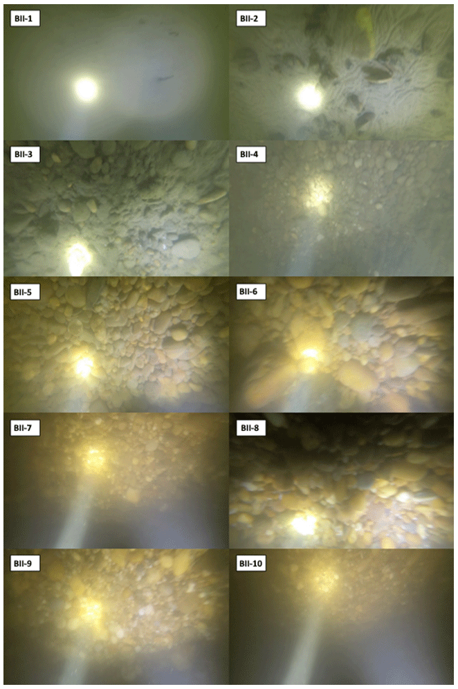
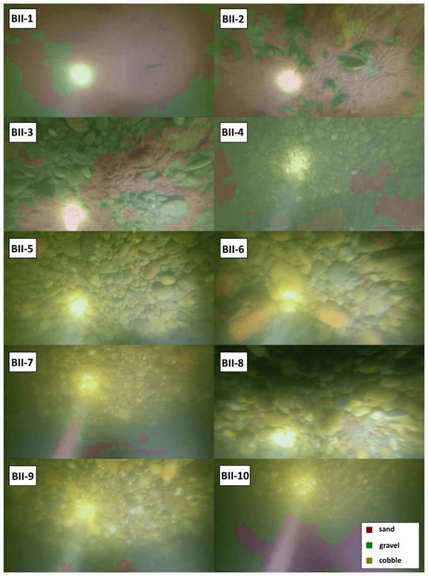
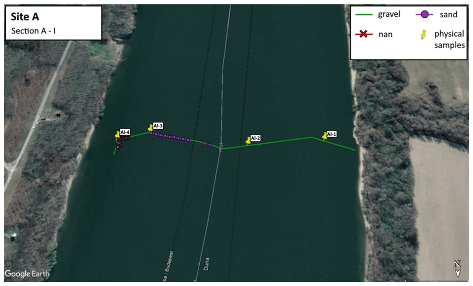
Figure C1 The path of the vessel and camera in Section A-I, Site A. The polyline is coloured based on the sediment seen during visual evaluation of the video. Yellow markers are the locations of physical bed material samplings (map created with © Google Earth Pro).

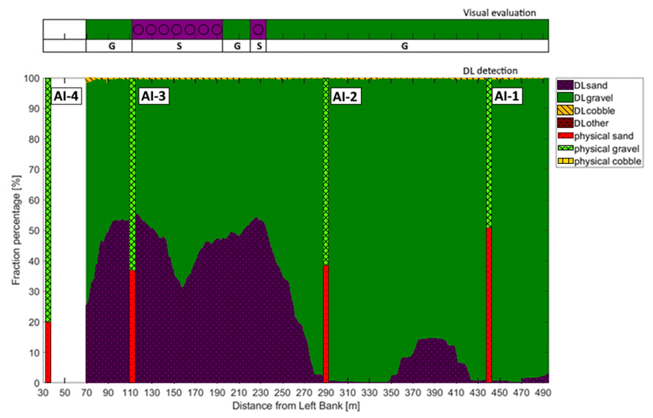
Figure C2 Sediment fraction percentages in Section A-I recognised by the AI. The visual evaluation included two classes: gravel is shown as G, and sand is shown as S. The fractions of the physical samples are shown as verticals.

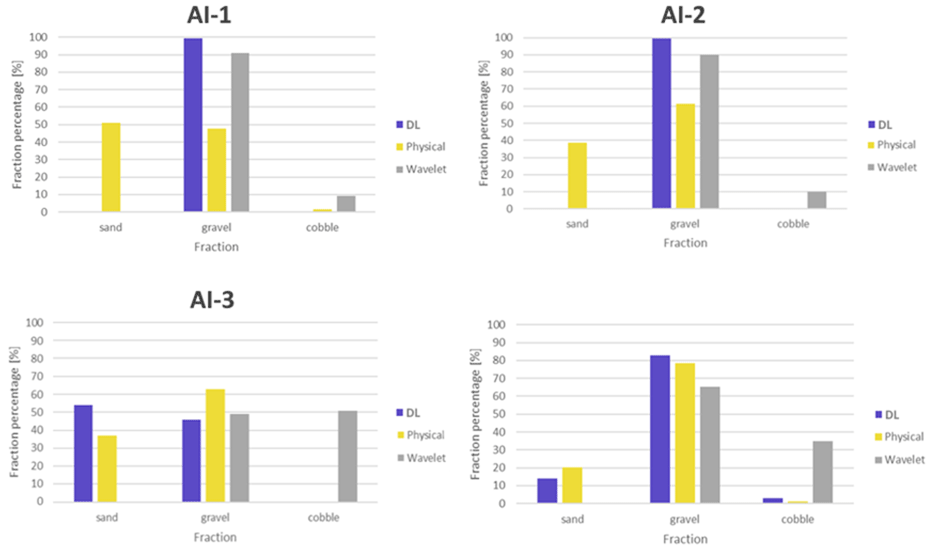
Figure C3 Comparison of sediment fraction (%) at the sampling locations from the moving-average DL detection, conventional sieving, and the wavelet-based image-processing method. Section A-I.

Figure C4 Riverbed video images at the sampling points in Section A-I.

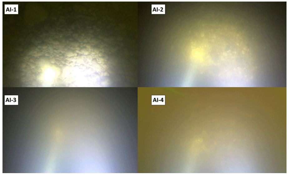
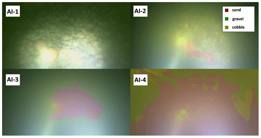
Figure C5 Riverbed video images overlapped with their raw, DL detection result at the sampling points in Section A-I.

Appendix D: Site A – Section A-III

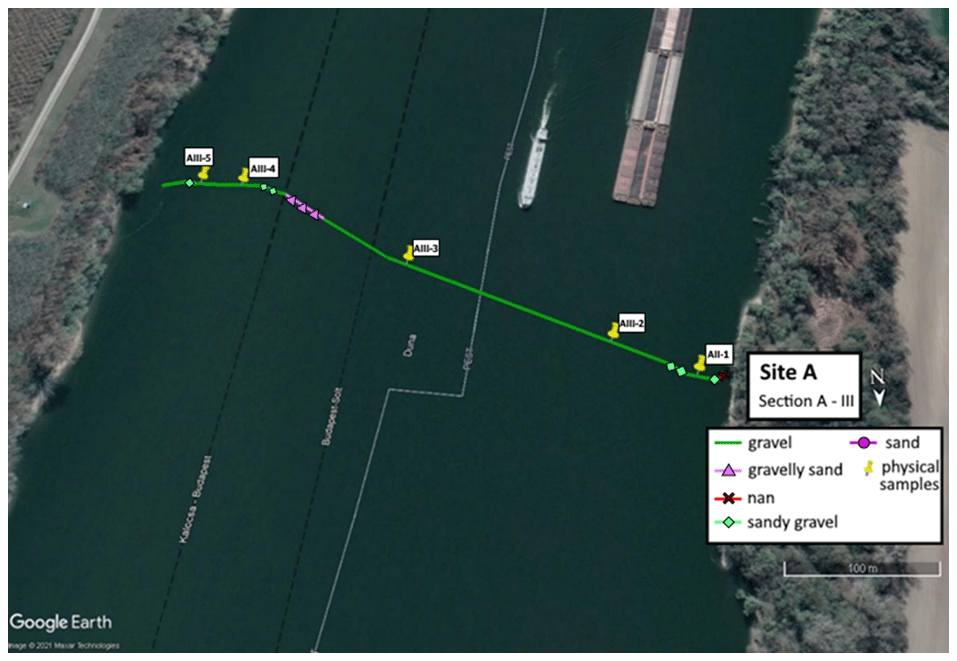
Figure D1 The path of the vessel and camera in Section A-III, Site A. The polyline is coloured based on the sediment seen during visual evaluation of the video. Yellow markers are the locations of physical bed material samplings (map created with © Google Earth Pro).

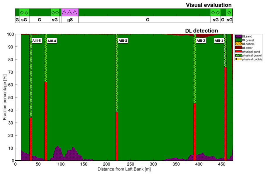
Figure D2 Sediment fraction percentages in Section A-III recognised by the AI. The visual evaluation included three classes: gravel is shown as G, sandy gravel is shown as sG, and gravelly sand is shown as gS. The fractions of the physical samples are shown as verticals.

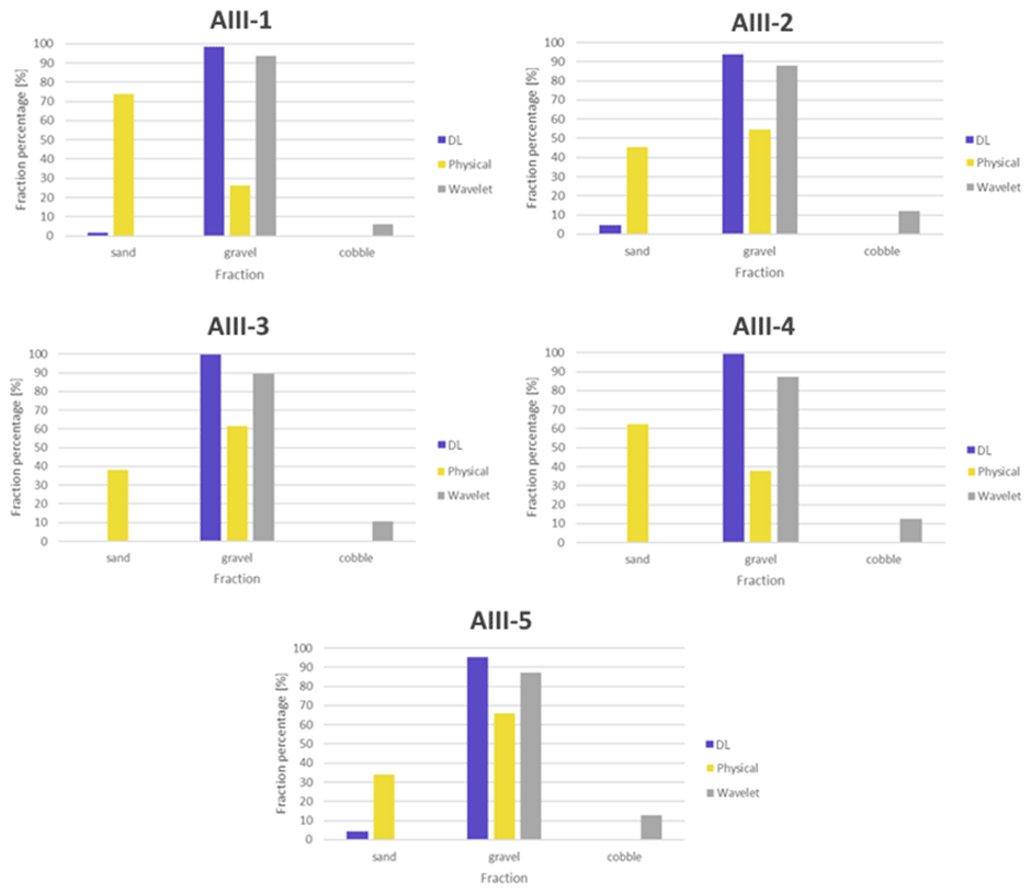
Figure D3 Comparison of sediment fraction (%) at the sampling locations from the moving-average DL detection, conventional sieving, and the wavelet-based image-processing method. Section A-III.

Figure D4 Riverbed video images at the sampling points in Section A-III.

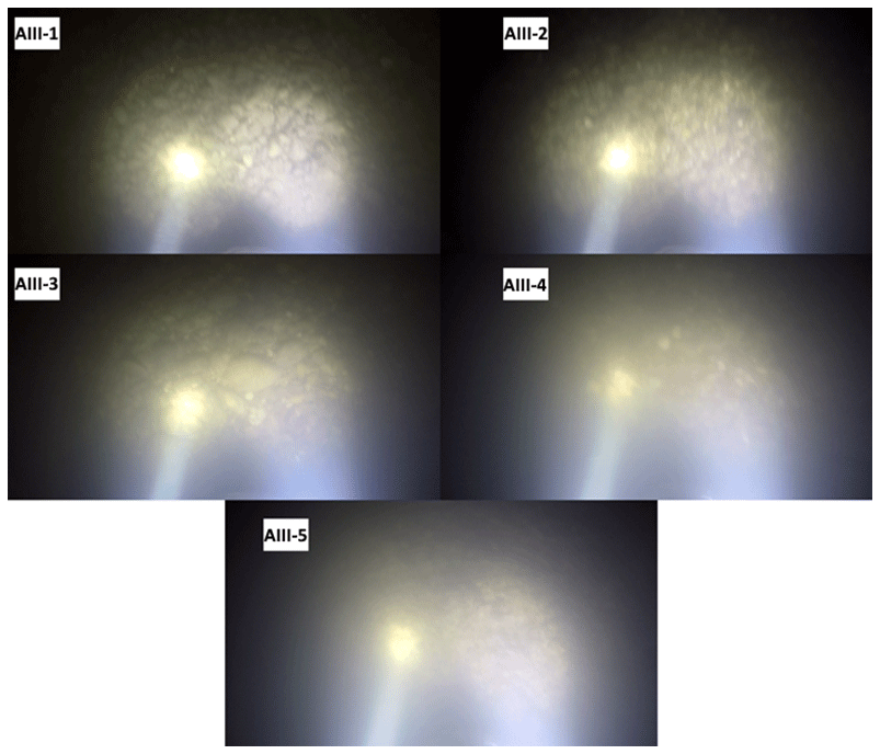
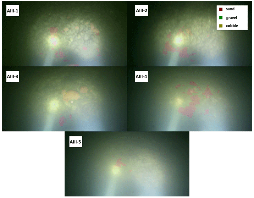
Figure D5 Riverbed video images overlapped with their raw, DL detection result at the sampling points in Section A-III.

Appendix E: Site B – Section B-I

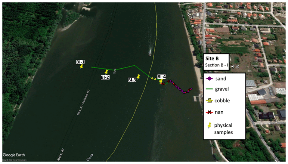
Figure E1 The path of the vessel and camera in Section B-I, Site B. The polyline is coloured based on the sediment seen during visual evaluation of the video. Yellow markers are the locations of physical bed material samplings (map created with © Google Earth Pro).

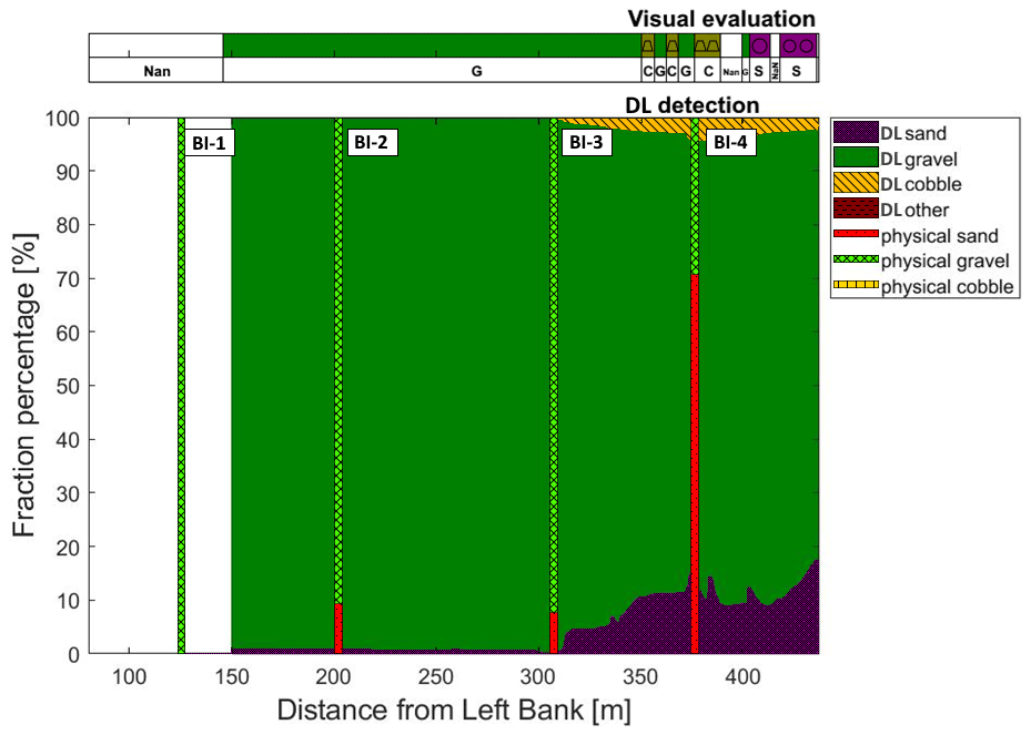
Figure E2 Sediment fraction percentages in Section B-I, recognised by the AI. The visual evaluation included two classes: gravel is shown as G, and sand is shown as S. The fractions of the physical samples are shown as verticals.

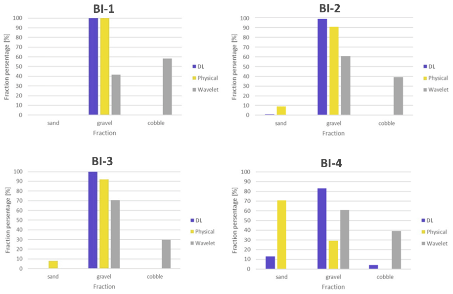
Figure E3 Comparison of sediment fraction (%) at the sampling locations from the moving-averaged DL detection, conventional sieving and the wavelet-based image-processing method. Section B-I.

Figure E4 Riverbed video images at the sampling points in Section B-I.

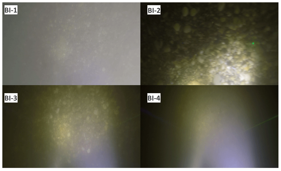
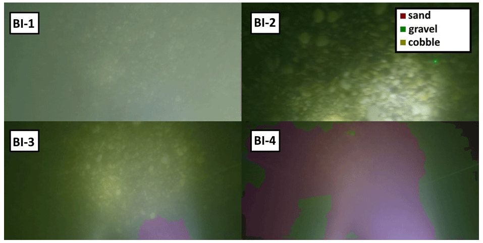
Figure E5 Riverbed video images overlapped with their raw, DL detection result at the sampling points in Section B-I.

Appendix F

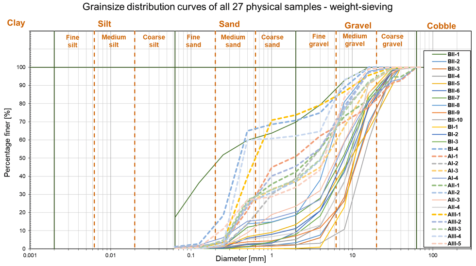
Figure F1 Grain size distribution curves of the 27 sieved physical samples; 11 curves categorised as Outlier Type-A are showcased with dashed lines. The shapes of these curves are representing bimodal (gap-graded) sediment distributions, which typically refers to bed armouring (i.e. excess of a certain particle size, a coarser surface layer protects a finer subsurface layer from being washed away). Hence, analysing images of the surface layer could not represent these complex distributions inherently.