Using repeat UAV-based laser scanning and multispectral imagery to explore eco-geomorphic feedbacks along a river corridor

Vegetation plays a critical role in the modulation of fluvial process and morphological evolution. However, adequately capturing the spatial and temporal variability and complexity of vegetation characteristics remains a challenge. Currently, most of the research seeking to address these issues takes place at either the individual plant scale or via larger-scale bulk roughness classifications, with the former typically seeking to characterise vegetation–flow interactions and the latter identifying spatial variation in vegetation types. Herein, we devise a method which extracts functional vegetation traits using UAV (uncrewed aerial vehicle) laser scanning and multispectral imagery and upscale these to reach-scale functional group classifications. Simultaneous monitoring of morphological change is undertaken to identify eco-geomorphic links between different functional groups and the geomorphic response of the system. Identification of four groups from quantitative structural modelling and two further groups from image analysis was achieved and upscaled to reach-scale group classifications with an overall accuracy of 80 %. For each functional group, the directions and magnitudes of geomorphic change were assessed over four time periods, comprising two summers and winters. This research reveals that remote sensing offers a possible solution to the challenges in scaling trait-based approaches for eco-geomorphic research and that future work should investigate how these methods may be applied to different functional groups and to larger areas using airborne laser scanning and satellite imagery datasets.

1 Introduction

Fluvial eco-geomorphic interactions are co-dependent, complex, and variable across space and time, representing a continued area of interest within river research (Thoms and Parsons, 2002). The diversity of eco-geomorphology in river corridors can be attributed to surrounding land use, existing morphology, and flood regimes (Naiman et al., 1993), whilst this same diversity simultaneously influences the flow of water and sediment, ultimately affecting morphology (Diehl et al., 2017a) and floodplain conveyance (Nepf and Vivoni, 2000). The role of vegetation within the river corridor is well established, benefiting the local ecology (Harvey and Gooseff, 2015; Sweeney et al., 2004) alongside playing a role in natural flood management schemes and reconnecting channels and floodplains (Lane, 2017; Wilkinson et al., 2019). This is important when considered against a backdrop of a rapidly changing climate where flow extremes are more varied, flooding is more likely (Unisdr and Cred, 2015), and riparian vegetation is likely to undergo shifts in composition (Rivaes et al., 2014; Palmer et al., 2009). Consequently, adequately measuring and monitoring vegetation within the fluvial domain are critical to understanding how these systems will respond to varying climatic and hydraulic conditions.

The characterisation of riparian vegetation distribution over larger (> 1 km) scales has typically relied upon the use of coarse classifications such as those identified in the Water Framework Directive (e.g. Gilvear et al., 2004) using techniques such as aerial imagery and satellite remote sensing (see Tomsett and Leyland, 2019). Advances in higher-resolution techniques, in particular mobile laser scanning, have enabled the possibility of capturing vegetation data in enough detail to establish individual plant structure (e.g. Brede et al., 2019; Hyyppä et al., 2020; Liang et al., 2014). Yet any characterisation must be scalable and geographically transferable to cover the vast range of different fluvial landscapes, whilst still accounting for the complexity presented within individual river corridors. Oversimplified, coarse classifications may altogether miss the complexity that exists, whilst conversely, highly detailed models tend to be necessarily localised and less transferable to alternate systems.

Trait-based classifications, developed and used within ecology, offer a scalable and transferable approach which can be applicable to the fluvial domain (Diehl et al., 2017a) and have been shown to be useful for modelling topographic response to changing vegetation, sediment, and flow conditions (Diehl et al., 2018; Butterfield et al., 2020). However, the application of trait-based classifications over larger reaches has yet to be fully realised due to the challenges in collecting appropriately high-resolution data at these scales (e.g. > 1 km). If such challenges can be overcome, it offers an opportunity for those analysing vegetation both within the river corridor and elsewhere in the landscape to obtain spatially explicit data on vegetation that were previously unattainable.

To address these gaps, we utilise remote sensing methods to collect data from which vegetation traits are extracted and assess how well these can be used to establish eco-geomorphic relationships. We use a UK-based temperate river as an example site to demonstrate the effectiveness of novel remote sensing techniques for characterising vegetation, investigating the limits of trait detection and the scales at which they are most appropriately used to enhance eco-geomorphic understanding.

1.1 The importance of vegetation

It is well understood that vegetation plays a key role within the river corridor and that how vegetation is represented in models (e.g. constant and varying roughness values, rigid cylinders) can affect the outcomes of hydrodynamic simulations. Channels with in-stream vegetation may experience roughness values an order of magnitude higher than non-vegetated channels (De Doncker et al., 2009), capable of reducing velocities by up to 90 % (Sand-Jensen and Pedersen, 1999), with stem shape, foliage, and deformation all influencing flow (James et al., 2008). The challenges posed by quantifying in-stream vegetation means that it is often difficult to make estimations of in-stream roughness (O'Hare et al., 2011). Conversely, terrestrial vegetation that influences flow during periods of flooding is easier to measure and monitor depending on the scales of analysis. Vegetation can reduce stream power, increase soil cohesion, and influence soil moisture levels, all of which can help to limit bank erosion (Simon et al., 2000; Fox et al., 2007; Kang, 2012). Bank collapse is influenced by three dominant factors, the extra mass of the vegetation, the shear strength provided by root reinforcement, and changes to bank pore water pressure (Wiel and Darby, 2007), with aboveground biomass therefore directly influencing the mechanical and hydraulic properties of the substrate (Gurnell, 2014). The aboveground biomass also has a direct influence on river flow and sediment transport when submerged (Gurnell, 2014), acting as a sediment trap and stabilising bars (Hortobágyi et al., 2018; Sharpe and James, 2006), although this is stage-dependent and varies with plant volume and structure. Therefore, being adequately able to capture such data over reach scales is critical for understanding the feedback loops between vegetation, flow, and morphology.

A functional-trait-based approach offers a way to represent vegetation data at reach scale and beyond. Functional traits originate from ecological research and are morphological, physiological, and phenological attributes that can be measured at the individual plant level (Violle et al., 2007; Kattge et al., 2011; Savage et al., 2007). These measured traits can either be an effect or response trait, whereby they either have an influence on or are influenced by their surrounding environment, respectively (Violle et al., 2007; Kattge et al., 2020). One of the benefits of collecting trait-based data is the ability to group plants that display similar functional traits into functional groups (Blondel, 2003). Herein we specifically use the term “functional group” (sensu Blondel, 2003) because we explore how aggregated ecosystem processes ultimately affect geomorphological response. This approach allows for increased applicability to different reaches that contain similar functional groups (Mcgill et al., 2006; De Bello et al., 2006; Garnier et al., 2006) and accounts for variation in local and regional conditions better than purely taxonomic approaches (Tabacchi et al., 2019).

Trait-based approaches are well suited for eco-geomorphic research due to the strong environmental gradients within fluvial systems (Naiman et al., 2005). Vegetation responds to hydrological variables, such as water availability and disturbance events (Hupp and Osterkamp, 1996), whilst also influencing flow, sediment transport, and morphological stability (Gurnell, 2014), meaning that the bi-directional nature of this relationship maps well onto a trait-based framework. Both plant form and distribution have been linked to stream power within the UK (O'Hare et al., 2011), with fluvial conditions also being shown to have a greater influence on trait composition than species composition (Göthe et al., 2017; Corenblit et al., 2015).

To date, most trait-based research has focused on ecological responses to environmental conditions. For example, greater inundation likelihood has been shown to increase the presence of plants with longer and younger leaves which are less woody, whereas plants in lower-stress environments tend to be taller with longer life cycles (Kyle and Leishman, 2009; Stromberg and Merritt, 2016; Mccoy-Sulentic et al., 2017). Furthermore, individual species have been shown to demonstrate differing traits depending on external stresses. Populus nigra trees were found to be smaller, have greater flexibility, and had a higher number of structural roots at a bar head when compared to a bar tail (Hortobágyi et al., 2017). Further work demonstrated that the trees located at the bar head were less effective at trapping sediment when compared to those at the bar tail (Hortobágyi et al., 2018). This highlights that the morphological response to vegetation may be harder to identify from taxonomic rather than trait-based approaches.

Research into effect traits and their geomorphic influence has received relatively less attention as trait concepts have only recently started to be explored within fluvial research. Temporally, changes in the dominant traits can lead to changing morphology (Manners et al., 2015), whilst spatially the location of dominant traits has been shown to alter morphological response, with combinations of different functional groups adding to the complexity (Hortobágyi et al., 2018). However, functional groups alone cannot explain all the variation in topographic response, with different groups in different locations under different hydraulic conditions exhibiting different topographic responses (Butterfield et al., 2020).

1.2 Hydraulically relevant traits

Not all vegetation traits are equally relevant when considering direct relationships between vegetation, river flow, and morphology. Moreover, not all traits can be obtained directly from remote sensing techniques, a necessary requirement when upscaling to larger domains. Below we briefly summarise vegetation traits that are highly relevant to fluvial environments and which have the potential to be captured via remote sensing techniques. These are based on Table 2 in Diehl et al. (2017a), which highlights the morphological effect of vegetation traits on geomorphic form.

Both plant height and frontal area are key traits which influence momentum exchange in river flows. The height of a plant will alter the extent of interaction it has with flow at various stages, whilst the submerged frontal area will impact the drag exerted on the water column (Nepf and Vivoni, 2000; Järvelä, 2004; Wilson et al., 2006). The frontal area of a plant will vary under different hydraulic conditions, making flexibility an important trait when investigating morphological response. Differences in foliated and non-foliated vegetation as well as woody and non-woody stems alter the thresholds in velocity at which deformation occurs (Wilson et al., 2003; Järvelä, 2002a; O'Hare et al., 2016; Sand-Jensen, 2003), modifying a plant's effective frontal area. However, the ability to obtain vegetation stem flexure directly from remote sensing is currently not possible, yet leaf area from remote sensing does show potential, and taxonomic approaches may better identify the “woodiness” of a species. Likewise, the vertical distribution of vegetation is important in determining the interaction between foliage and flow stage (Lightbody and Nepf, 2006; Jalonen et al., 2012), which can be obtained from remotely sensed data.

At patch scales, the density and configuration of plants can impact the resultant drag. The non-equivalence between the drag induced by individual plants compared to those in bulk vegetation requires the inclusion of bulk factors in vegetation analysis (James et al., 2008). Higher densities of plants will lead to an increase in drag, with differences in the arrangement and density of patches causing variation in the resultant reduction in water velocities (Järvelä, 2002b; Kim and Stoesser, 2011; Sand-Jensen, 2008), highlighting the need to account for plant spacing when examining changes in morphology, which remote sensing is capable of achieving. At the reach scale, functional groups have an aggregated response in modulating scour or deposition and resultant planform morphology. Vegetation dynamics have been previously described using trait-based frameworks in fluvial systems (Diehl et al., 2017a, 2018; Butterfield et al., 2020), with a wealth of studies showing the wider impact that vegetation has on planform morphology and erosion in flumes (Van Dijk et al., 2013; Coulthard, 2005; Bertoldi et al., 2015), modelling studies (Oorschot et al., 2016; Crosato and Saleh, 2011), and field-based research (Bywater-Reyes et al., 2017; Diehl et al., 2017b).

Whilst we have focused on hydraulically relevant traits that can be measured using remote sensing techniques, Diehl et al. (2017a) present others which cannot be easily obtained from the remote sensing techniques outlined below. Factors such as plant biomass, buoyancy, and root architecture are all outlined as having a role in affecting subsequent morphology (Sand-Jensen, 2008; Abernethy and Rutherfurd, 2001; De Baets et al., 2007). This highlights the potential role of taxonomic approaches alongside the measurement of structural data to both capture the variability where possible and enhance this with wider datasets for traits that cannot be remotely sensed but are still relevant to morphology.

1.3 Remote sensing for trait data collection

Although some traits are inherently measurable in the field, many of them are not obtainable from current remote sensing methods. Direct trait extraction for riparian vegetation from airborne (i.e. large-scale) remote sensing has not yet been used within eco-geomorphic studies. Currently, the collection of trait data relies on ground-based field surveys using quadrat or transect sampling as well as lab analysis or species being identified in the field and traits inferred from lookup tables, such as the TRY database (Kattge et al., 2020). This technique is effective for establishing traits but is limited by the spatial extent of ground coverage. Within fluvial research, multispectral imagery has been collected to determine plant species which are then used to identify dominant traits via supervised and unsupervised classifications (Butterfield et al., 2020). Outside the fluvial domain, several efforts have been made to utilise remote sensing methods for trait extraction using a mix of terrestrial, airborne, and satellite platforms (Anderson et al., 2018; Valbuena et al., 2020; Zhao et al., 2022; Aguirre-Gutiérrez et al., 2021; Abelleira Martínez et al., 2016). However, limitations still remain despite these efforts due to the uncertainty in relating spectral and physical properties to functional traits (Houborg et al., 2015).

Yet, considerable advances continue to be made in using remote sensing to monitor riparian vegetation at a range of scales. Advances in UAV (uncrewed aerial vehicle) remote sensing can offer a way of bridging the scales from ground surveys to larger extents. UAV data collection allows high-resolution imagery and active remote sensing methods such as laser scanning to be conducted on large reaches relatively easily (Tomsett and Leyland, 2019), increasing coverage and providing a middle ground for relating local- to large-scale data. Multispectral cameras have already helped to improve the classification of vegetation from UAVs (Al-Ali et al., 2020), with active UAV-LS (UAV laser scanning) being shown to be comparable in estimating tree structures to terrestrial laser scanning (TLS) methods (Brede et al., 2019; Hillman et al., 2021) and a combination of both techniques helping to improve tree crown delineation and biomass estimates (Dersch et al., 2023; Lian et al., 2022; Dash et al., 2019). TLS has become the benchmark technique from which to obtain highly accurate vegetation data (Bywater-Reyes et al., 2017; Jalonen et al., 2015; Lague, 2020) yet still suffers from issues of occlusion and limited spatial extent in comparison to mobile techniques. Airborne laser scanning (ALS) can be used to classify different vegetation regimes, classifying different woodland types (Stackhouse et al., 2023) and identifying differences in species using intensity data (Donoghue et al., 2007), but obtaining temporally relevant data at adequate point densities is challenging.

The survey techniques outlined above present an opportunity to not only classify vegetation by type and assign them to functional groups, but also to define these very groups based on characteristics acquired directly from remote sensing before upscaling them to reach-scale classifications. Moreover, a key advance in using UAV-based methods for collecting vegetation data is the spatial resolution at which functional groups can be discretised and the temporal resolution which can be achieved by undertaking multiple repeat surveys. Such surveys can allow for both leaf-on and leaf-off conditions as well as the emergence of perennial vegetation, avoiding the need to make any assumptions about the phenological cycle. Consequently, identifying whether it is possible to obtain trait data from various remote sensing sources, upscale these to reach-scale metrics, and examine links to geomorphic activity is underexplored.

1.4 Aims

The aim of this research is to use UAV-derived and terrestrial 3D datasets to develop a workflow and methods which are able to extract relevant plant traits to explore the spatial and temporal variation and importance of eco-geomorphic interactions on a UK river system. This is achieved using the following specific objectives:

1. Develop a methodological workflow to identify and select hydraulically relevant traits extracted from high-resolution remote sensing data.

2. Establish the presence of functional groups (those with similar traits) for the river reach using exploratory analysis and machine learning.

3. Examine links between the spatial variation in functional groups and morphological change across a 2-year period to identify any eco-geomorphic feedbacks that may be present.

2 Study site

The study site is located on the upper course of the River Teme on the English–Welsh border in the UK (Fig. 1a). The reach consists of two distinct sections: an upstream section consisting of open grassland with patches of heterogeneous vegetation and a downstream section which flows through denser vegetation and woodland. The River Teme is a highly mobile gravel-bed river within an alluvial floodplain which exhibits numerous historic avulsions, typical of many UK rivers. There is active lateral erosion of the channel, depositional gravel bar features, and woody debris dams across the study site (Fig. 1b). Since 2002, the reach has typically had low flows (Fig. 1c), with an average depth of 0.69 m (±0.15 m) throughout the year with slightly higher average flow depths in the winter months (November–February, 0.79 m ± 0.15 m). A total of 95 % of river depths have been below 0.99 m and 99 % of the flow depths have been below 1.48 m. The largest recorded river depth was 2.85 m on 16 February 2020 during Storm Dennis.

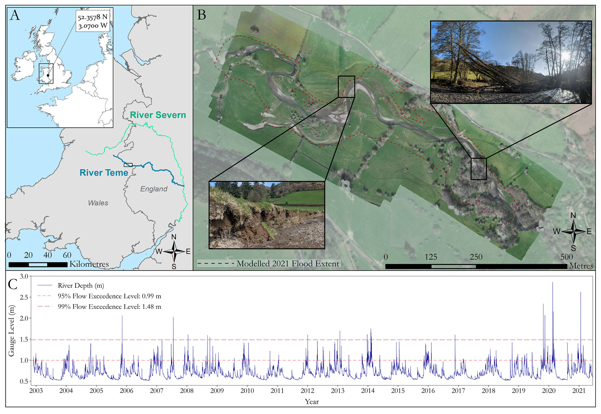
Figure 1 (a) Study site location on the River Teme, UK. Inset country outlines provided by EUROSTAT (2020) and UK outlines provided by the UK Office for National Statistics (2019). (b) Plan view of the reach with inset images showing active bank erosion and a large debris dam caused by falling trees. The red dashed outline indicates the flood extent modelled within this study. Ortho-imagery collected in February 2020 and background imagery provided by Esri (2021). (c) River gauge level at the Knighton monitoring station ∼ 2 km downstream from the study reach (data available from 2002–present, operated by the UK Environment Agency).

3 Methods

3.1 Field collection of high-resolution 4D data

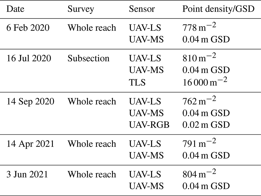
A series of six high-resolution UAV-LS (UAV laser scanning) and UAV-MS (UAV multispectral) surveys were collected over the entire reach shown in Fig. 1 from February 2020 until June 2021. To complement these flights, a single terrestrial laser scanning (TLS) survey using a Leica P20 was undertaken of vegetated and bar sections in July 2020 to gain a benchmark ultrahigh-resolution dataset for characterising small herbaceous vegetation, co-registered to an accuracy of ±0.007 m with georeferenced scan targets. UAV-RGB (red, green, blue) surveys were also undertaken in September 2020 for classification validation. Table 1 summarises the survey dates, extents, data collection methods, and point density for UAV-LS and GSD (ground sampling distance) for UAV-MS and UAV-RGB. A detailed outline of the UAV-based sensor setup, processing routine, and accuracy assessment can be found in Tomsett and Leyland (2021a). All data were processed in the WGS UTM Zone 30N coordinate system.

Table 1 Data collection methods, extent, and point density for each survey date. TLS point density is based on the resultant point cloud after registration. UAV-LS point density is determined after cleaning of the raw clouds has taken place. Ground sampling distance (GSD) is the resolution of the resultant orthomosaics.

3.2 Vegetation functional trait extraction

The workflow developed to extract plant functional traits consisted of five steps: (1) separation of individual plant point clouds from the UAV-LS data from February 2020 and TLS data from July 2020, (2) analysis of these individual clouds to extract metrics related to their traits, (3) separation of plants into functional groups adapted from Diehl et al. (2017a) based on similar traits, (4) identification of functional group reach-scale properties from UAV-LS and UAV-MS datasets from 2020, and (5) use of an object-based random forest classifier to determine the spatial discretisation of these functional groups for both 2020 and 2021. These steps are outlined in the following sections and are shown as a processing workflow in Fig. 2 to provide context in relation to which surveys contributed to each element of the analysis. Figure 2 also shows how the resultant functional groups are used in conjunction with the morphological change detection.

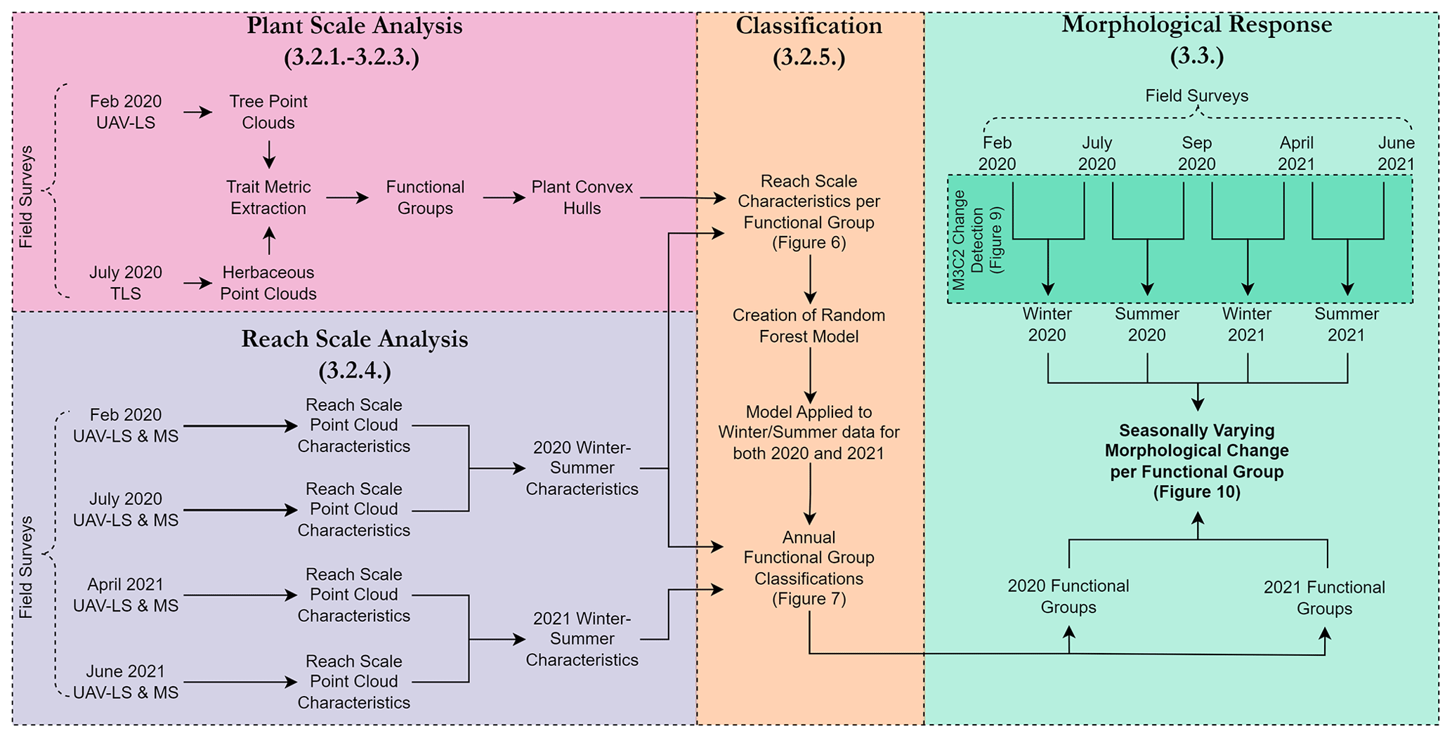
Figure 2 An overview of the workflow. used to process collected field data (Table 1) through to analysis of morphological change for each functional group. Each colour block indicates a different stage of the analysis which corresponds to the numbered sections that follow.

3.2.1 Point cloud segmentation

A number of automatic methods exist to classify very dense point cloud scenes into different groups (e.g. Brodu and Lague, 2012; Zhong et al., 2016). However, the majority of these are designed for ultrahigh-resolution TLS datasets rather than UAV-LS (see Table 1 for density metrics), so a semi-automated approach was employed. Smaller vegetation, where the structural composition cannot be fully resolved from UAV-LS data, was analysed from the July 2020 TLS survey, whereas larger vegetation was analysed in leaf-off conditions from the February 2020 survey. Automatic classification of ground and non-ground points was performed using the progressive morphological filter in the LidR package (Roussel et al., 2020) before manually segmenting in CloudCompare (https://www.danielgm.net/cc/, last access: 1 December 2020) to create individual plant models (Fig. 3, raw point cloud).

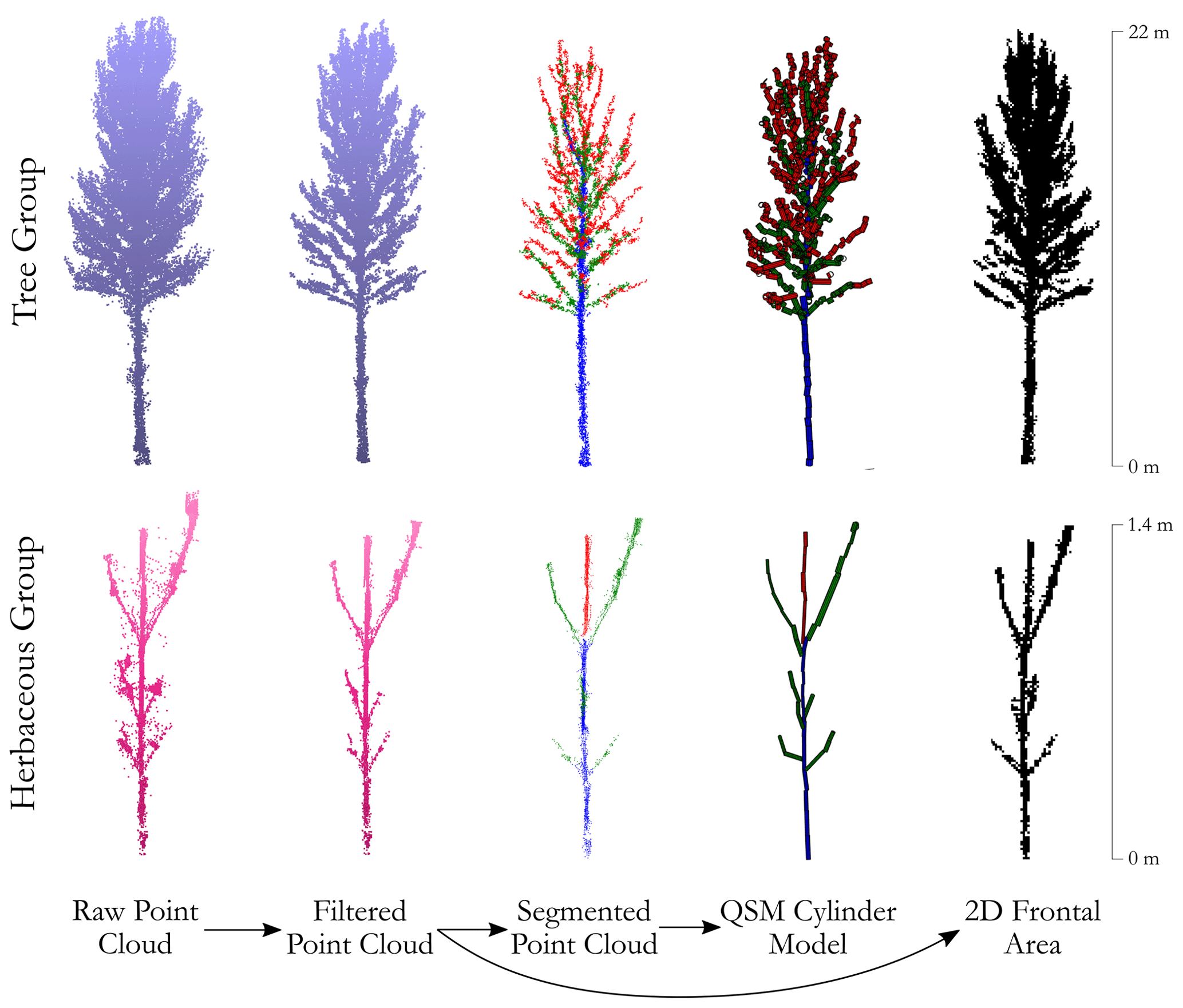
Figure 3 Vegetation trait extraction from an individual raw plant point cloud to a cylindrical model and frontal area. The process is demonstrated for two extracted vegetation point clouds, a large tree within the study reach collected from UAV-LS data, and a perennial on the central bar collected from TLS; note the difference in scales. The segmented point cloud is coloured by branching order from blue to green to red, with the cylinders coloured in the same manner. The 2D frontal areas are based on the filtered point clouds rather than the segmented point clouds or QSM cylinder models, and as such these steps are not required to compute the frontal area data.

For the herbaceous plants in the TLS data, leaves and flowering parts were manually removed from the clouds so as not to influence the quantitative structural modelling (QSM; see Sect. 3.2.2). This was done based on field images and the appearance of the clouds to leave just the structural components. Although foliage has previously been shown to be important (Järvelä, 2002a; Whittaker et al., 2013), for the methods used herein it could not be fully resolved due to insufficient point densities. Any statistical outliers were then detected and removed from the dataset using the in-built tools within CloudCompare, identifying points > 2.5 standard deviations above the mean separation distance between points within the segmented cloud. This process was repeated for plants found within the TLS scans of the study site, resulting in a sample dataset consisting of 37 herbaceous plants. Plants that were selected from the TLS point cloud represented complete vertical profiles to minimise the effect of shadowing from different scan angles.

Tree segmentation also consisted of a combination of manual and automatic classification based on surveys undertaken in leaf-off conditions to expose the full tree structure. A total of 24 trees were selected from across the reach, representing a range of structures and sizes from which complete models could be created. Trees were manually extracted prior to interactive filtering using a number of statistical measures; local volume density helped to separate points distinct from the main tree woody structure, whilst linearity metric filters (how aligned points are within a set radius) remove points that are highly complex or not part of the main tree structure. The statistical outlier removal tool and a final manual check can then be used to remove any remaining points. This resulted in a point cloud of predominantly large branches, with a clearer structural profile as can be seen in Fig. 3 (filtered point cloud). The thresholds for separating individual trees are size-, structure-, and point-density-dependent, hence the need for interactive selection. Although this adds an element of user bias as to what is deemed a “main” branch, the lower density of UAV-LS scans makes user input necessary before reconstructing vegetation models (Brede et al., 2019).

Shrubs and grasses whose structure could not be fully resolved from the UAV-LS or TLS data were not analysed for trait extraction. Grasses are typically too short to remotely sense with high degrees of confidence, and the complex and extensive nature of the branching network of shrubs would require several TLS scans per plant, with numerous plants needing to be surveyed to get a reliable trait description (Vasilopoulos, 2017). As a result, point clouds for shrub classes were only used for classification training, frontal area, and density calculations.

3.2.2 Trait metric extraction

The hydraulically relevant traits collected were based on those noted within Diehl et al. (2017a), which could also be measured using the remote sensing methods available to us within this study. These were plant height, number of branches, maximum branching order, stem diameter, plant volume, frontal area, and plant density.

For the reconstruction of vegetation stems into cylindrical models, the open-source TreeQSM method (Raumonen et al., 2013) was applied to the segmented UAV-LS- and TLS-derived individual plant data from 2020 as outlined above. TreeQSM utilises “patches” to determine connected points in the vegetation cloud before growing the tree structure by joining patches together to form a complete model (Raumonen et al., 2013). These are created using user-defined initial patch sizes to adjoin points before refining the patch sizes using minimum and maximum limits to create a complete model. This allows the coarse branch structure of the tree to be identified (Fig. 3, segmented point cloud). Sections are then reconstructed as cylinders, both for computational efficiency and because they provide a robust representation of trees (Raumonen et al., 2013). The cylinders are then used to describe the overall structure and properties of the individual plant (Fig. 3, QSM cylinder model). A full method description can be found in Raumonen et al. (2013). QSM methods have been noted to overstate the volume of smaller branches and are sensitive to noise in the data alongside variable point density (Fang and Strimbu, 2019; Hackenberg et al., 2015). However, QSM reconstructs plant structures in a manner which resolves many of the hydraulically relevant vegetation traits, making it a suitable approach for this research.

Patch diameters (which are used to determine adjacent points within the same tree) were chosen following a parameter sensitivity exercise, with the range of values initially based around those of Raumonen et al. (2013) and Brede et al. (2019) for TLS and UAV-LS approaches, respectively. A visual assessment was performed to identify parameters that created models similar to the observed vegetation structure. After testing for the optimum patch sizes, the TLS scans of herbaceous vegetation initial patch diameter were set at a size of 0.005 m, with the second patch diameter minimum and maximum sizes of 0.002 and 0.01 m. The minimum cylinder radius was set to 0.005 m, prescribing the smallest detectable branch structure of the extracted herbaceous plants. For the UAV-LS-derived tree data, the initial patch diameter was 0.2 m, with the second patch diameter minimum and maximum sizes of 0.1 and 0.5 m. The minimum cylinder radius was 0.1 m based on manual measurements of tree branches within the point cloud that were detectable. For each individual plant model the cylinder reconstruction and variable extraction were repeated 10 times. As the modelling begins at a random location each time, the start point can affect the results, so multiple averaged simulations provide a more representative solution. The modelling produces a number of metrics, but for this study hydraulically relevant traits of plant height, number of branches, stem diameter, volume, and maximum branching order were collected. For each metric of interest, the average value and standard deviation of these values are taken from the 10 runs.

The frontal areas of all segregated vegetation clouds were extracted alongside the construction of the cylinder models based on the 2D methods described by Vasilopoulos (2017). For each discretised filtered plant point cloud (Fig. 3, filtered point cloud), the data were flattened from 3D to 2D by collapsing the data along a single horizontal dimension on a regular grid (Fig. 3, 2D frontal area). The grid resolution was set at half the width of the minimal detectable feature resolved by the QSM: 0.0025 m for the TLS-derived herbaceous plants and UAV-LS 0.05 m for UAV-LS-derived trees. Each plant was flattened along the x and y axis, respectively, with an average frontal area taken.

In the absence of manually collected field validation data, to assess the ability of the UAV-LS to capture vegetation properties and for the QSM to produce reliable models, a series of checks were undertaken. First, UAV-LS tree heights and diameter at breast height (DBH) from February 2020 and April 2021 were compared to trees that were also captured in the TLS scans from July 2020. It is assumed that differences in tree height and DBH between these surveys due to the temporal offset would be negligible. This provides an estimation of how well UAV-LS captures tree properties compared to the benchmark high-resolution techniques (Kankare et al., 2013; Hillman et al., 2021; Calders et al., 2015; Brede et al., 2019). For both the herbaceous and tree plants within the QSM analysis, the modelled plant heights and DBH were compared to measured values from each plant's point cloud, with DBH being measured across two perpendicular axes to obtain a mean diameter for the point cloud. Finally, available databases and the wider literature were used to ensure values were within the expected range for each species measured at other sites (see Sect. 4.2.1).

3.2.3 Identification of functional groups

For the separated individual plant point clouds, each was assigned to a functional group adapted from those outlined in O'Hare et al. (2016) and Diehl et al. (2017a). These groups were grasses, short branching herbs, tall single-stemmed herbs, shrubs and bushes, low-DBH trees, and high-DBH trees. As discussed previously, shrubs and grasses were not identified using trait extraction. Short branching herbs and taller single-stemmed herbs were separated due to the likely variability in flexibility, branching architecture, and height, all of which interact differently with flow. Large woody vegetation was split into two functional groups, those with high diameter at breast height (DBH) that had a low density of plants and those with lower DBH that had a higher plant density, to account for the different interactions with overbank flow.

To assess whether remotely sensed data could separate out plants into their functional groups in a statistically robust way, a principal component analysis (PCA) was undertaken to identify the variables which explained most variation within the derived trait metrics. The metrics used for the PCA were those obtained from the QSM and frontal area calculations outlined above, which were normalised to remove the influence of different scales (Alaibakhsh et al., 2017). The principal components identified were used to inform the classification of reach-scale functional groups, identifying those variables that most explained the variation between groups. The PCA was performed separately on the two herbaceous groups and the two woody groups, as although height would clearly be a dominant variable between these two groups, it would not necessarily be one within the groups. All of the herbaceous point clouds from the summer 2020 TLS survey were used in the herbaceous group PCA, and all the high- and low-DBH tree point clouds from the winter 2020 UAV-LS data were included in the woody group PCA.

3.2.4 Traits and land cover metrics at the reach scale

To scale the analysis from individual plants to the entire reach level, a method of linking plant-scale traits to reach-scale data is required. Convex hulls representing the spatial extent for each plant-scale vegetation point cloud analysed above were used to define the regions from which UAV-LS and UAV-MS data were extracted. For small herbaceous vegetation, this was buffered by 0.25 m to account for any misalignment between TLS and UAV-LS clouds. For tree vegetation polygons this buffer was increased to 1 m to incorporate peripheral branches and leaves removed during point cloud filtering. A total of 11 polygons for shrubs and bushes were created based on field notes from various surveys and photographs from the summer surveys, their outlines in the UAV-LS point clouds, and UAV-MS imagery. Similarly, 11 polygons were defined for grasses. In addition to these vegetation functional groups, eight polygons for water classes and five for a combined gravel bar and bare earth class were also created using the same technique to classify the remaining land cover. Within these polygons, leaf-on and leaf-off variables were extracted for scaling plant-scale functional group identification to reach-scale classification.

The structural characteristics of the reach-scale point clouds were extracted through TopCAT (Brasington et al., 2012), obtaining the standard deviation, skewness, and kurtosis over a sampled grid at 1 and 4 m resolutions, the latter to account for larger vegetation footprints. The 4 m resolution grid only considered points classified as vegetation to remove ground points. To extract a canopy height model (CHM), a bare earth digital terrain model (1 m resolution) was subtracted from a digital surface model (0.25 m resolution) incorporating the vegetation points. The normalised difference vegetation index (NDVI) across the reach was calculated using the red band along with both the red-edge and near-infrared bands of the MicaSense orthomosaic images to produce two separate NDVI layers. As the red edge can be used to separate out vegetation signatures, using a combination of both was expected to help differentiate plants with similar structural but different spectral properties (Schuster et al., 2012; Guo et al., 2021). For each of the vegetation convex hulls, the attributes of the structural and spectral layers for leaf-on and leaf-off conditions were extracted. The mean and standard deviation for each attribute for each survey were then calculated across the different functional groups for use in the classification model.

3.2.5 Reach-scale functional group and land cover classification

To transition from plant-scale groups created from individual UAV-LS and TLS clouds to reach-scale analysis, an object-based random forest classification was undertaken. Object-based approaches overcome some of the issues of variation and complexity in high-resolution images (Myint et al., 2011), improving continuity in the results (Duro et al., 2012; Wang et al., 2018). The RGB bands from the multispectral camera and the CHM were combined to create a four-layer image from which to identify distinct objects in summer imagery for both 2020 and 2021. The Felzenszwalb algorithm was applied, which uses graph-based image analysis to segment an image into its component parts based on the pixel properties (Felzenszwalb and Huttenlocher, 2004). This results in regions within the image being grouped based on them having similar properties according to the input layers, avoiding the salt-and-pepper effect found in traditional pixel-by-pixel classification approaches (Wang et al., 2018).

In total, 644 training objects were identified for the 2020 summer imagery, with the previously discretised vegetation convex hulls having multiple training objects present within each sample (Table 2). A random forest classifier was then trained using these 2020 data. The reach-scale structural and spectral datasets created in Sect. 3.2.4 were used to train the model, alongside an additional water mask layer created from the multispectral imagery to account for varying flow stages. Data from leaf-on and leaf-off conditions were used for each year's classification, with an annual map being constructed. This was chosen due to the need for both summer and winter data to classify different functional groups. This helps to improve confidence in the classification where variation in reach-scale metrics happens both between groups and between seasons. Although leaf-on and leaf-off data with no geomorphic change between surveys would have been favourable, the combination of datasets where geomorphic change had occurred is unavoidable based on the survey dates.

Table 2 Description of functional groups and land cover classes used for training the random forest classifier, showing the number of training objects from the image segmentation for 2020 imagery and the training area size.

An analysis of model accuracy vs. the number of forests showed a convergence of accuracy above 100 forests and a reduction in band importance variability above 300 forests. Higher variation in band importance suggests that the number of trees is influencing the likelihood of an optimal solution. This random forest classification (no. trees 300) was then applied to the remaining unclassified objects within the reach for 2020 and also for all objects in the segmented 2021 data.

Due to the limited number of extracted samples from the point clouds, there were not enough to split into a training and test dataset. The multi-tree approach of random forests is constructed on a sample of the dataset and as such can be tested against itself to determine an out-of-bag accuracy score. It also successively adds and removes bands to determine the band importance in the classification (Adelabu and Dube, 2015). Alongside this model self-assessment, for the final functional group classes a total of 80 random points were generated across the study site with an equal number in each outputted group. These were manually classified using high-resolution ortho-imagery from a UAV-RGB (0.02 m resolution) survey from September 2020, field photographs, and study site knowledge. The output classification was not visible when undertaking this accuracy assessment, and the order of the control points was shuffled to remove user bias. The classification map produced for 2020 was then compared to the manually classified control points before a confusion matrix was utilised to assess the accuracy of the classification.

3.3 Morphological change

The M3C2 algorithm (Lague et al., 2013) was employed to calculate morphological change, whereby the surface normals from a subsampled cloud of core points (here at 0.1 m resolution) are calculated, and change along the normal direction is identified with the calculation of a local confidence interval. This overcomes some of the limitations of traditional elevation model differencing which cannot account for the direction of change, a problem that is pronounced, for example, on the vertical faces of riverbanks (Leyland et al., 2017). The benefits of using both structure-from-motion (SfM) and UAV-LS data allow their respective drawbacks to be overcome through combining datasets. SfM has been shown to perform poorly in vegetated reaches where UAV-LS maintains good ground point densities, yet SfM provides good continuity and high point densities in unobstructed areas. Therefore, to ensure the creation of robust surface normals, both the UAV-LS and UAV-SfM clouds were merged for each survey date (see Tomsett and Leyland, 2021a, for error analysis) and their vegetation was removed. These resultant clouds were then differenced from their preceding survey date using the M3C2 algorithm.

4 Results

4.1 Hydraulically relevant trait analysis

4.1.1 Trait extraction error and uncertainty

The repeat QSM of the individual plants produced consistent trait results. The heights of herbaceous groups were consistent to within 4 %, whilst tree groups were consistent to just over 1 %. Repeat diameter calculations were within 16 % (0.08 m) for tree groups and within 18 % (0.002 m) for herbaceous groups. Higher discrepancies were found in the number of branches; for trees, the numbers of branches for each model repeat were within 9 % of each other, equivalent to 12 branches, whereas for herbaceous functional groups this was 17 %, which equates to under 1 branch. The complexity of the larger tree models makes this variation quite likely, especially when the resolution of branches approaches the resolution of the scan data, whereas for herbaceous groups the higher variation is a result of the low number of total branches, so an additional branch being identified has a large impact on the results.

When comparing data measured by TLS and UAV-LS (Fig. 4a), the UAV-LS performs well, averaging 100.4 % ± 1.8 % of TLS heights and 103.8 % ± 11.2 % of TLS DBH values. Discrepancy in the latter may also be influenced by incomplete trunk reconstructions from the TLS scans, which did not always capture the full trunk profile. The RMSE in TLS vs. UAV-LS DBH was 0.094 m, which is within the same order of magnitude of error identified by Brede et al. (2019). When comparing reconstructed QSM values to those measured directly in CloudCompare, values for both height and DBH align well (Fig. 4b). Across all groups, average percentages of reference heights were 100.2 % ± 2.04 % and for DBH were 100.2 % ± 10.9 %. The greater variation in DBH for herbaceous groups alone (±12.01 %) is likely due to the stem widths being closer to the precision of the TLS, with any error from manual diameter measurements having a greater impact on comparisons between modelled and referenced data. This suggests that the UAV-LS and QSM methods used reconstruct plant structure well for extracting traits and are suitable for this methodological approach.

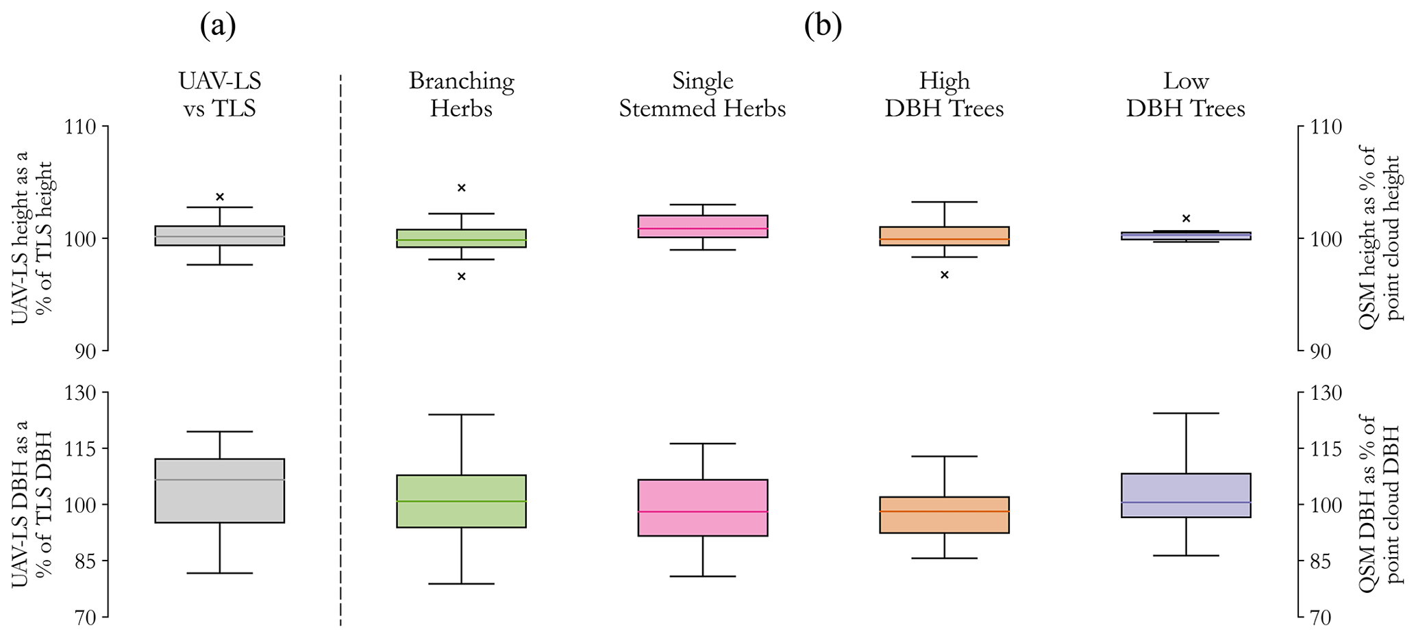
Figure 4 (a) Differences in UAV-LS-derived height (top) and DBH (bottom) as a percentage of TLS values for the same trees (n=14), demonstrating good agreement in height and a slight overestimation in DBH from UAV methods. (b) Differences in QSM height (top) and DBH (bottom) as a percentage of measured point cloud data for each of the four functional groups modelled (n=48). Height values are again closely matched, with greater variation in DBH values.

Finally, values extracted from the survey data were compared to those found in the wider literature and online databases. Within the tree functional groups, those with a low DBH had an average height of 18.2 m ± 3.3 m and a DBH of 0.39 m ± 0.08 m. Field identification from photos taken on site identified a large number of these trees to be of the poplar variety (e.g. Populus alba), and comparisons with both the TRY database (Kattge et al., 2020) and observations in the literature comparing height and DBH for these species showed good agreement (e.g. Burgess et al., 2019; Engindeniz and Olgun, 2003; Zhang et al., 2020). Trees with a higher DBH were predominantly identified as a mix of willow (Salix alba) and alder (Alnus glutinosa), with average heights of 14.9 m ± 3.2 m and with average DBH values of 0.69 m ± 0.11 m. This aligned well with the overall height ranges observed in the TRY database for alder trees, with the only record with both height and DBH values for alder showing a tree of 30 m having a DBH of 0.9 m. Southall et al. (2003) found diameters of willows up to 0.45 m for plants 8–9 m in height, with the trees in this study being both taller and larger in diameter, suggesting a difference in maturity. Conversely, both Colbert et al. (2002) and Jurekova et al. (2008) found DBH values for willow within the observed range of diameters in this study for trees of similar height. This suggests that although the original QSM methods were tested on fir, spruce, beech, and oak trees, the methods are suitable for use on a wider variety of plants and produce results in line with those expected for the species being observed.

Field observations of the single-stemmed herbaceous group identified a dominance of marsh thistle (Cirsium palustre), with average heights of 1.14 m ± 0.17 m and an average stem diameter of 0.013 m ± 0.002 m. Height values align well with those found in the TRY database, with the majority of recorded heights between 0.8 and 2 m (Kattge et al., 2020). Van Leeuwen (1983) measured stem circumferences of 0.026–0.070 m, equating to diameters of between 0.008 and 0.022 m, yet very little other literature and very few values on stem circumference or diameter are available. Likewise, comparison between the average height values of the branching herbaceous group, predominantly identified as hedge mustard (Sisymbrium officinale), and those values in the TRY database indicate good agreement, with reconstructed values from the field having heights of 0.46 m ± 0.12 m and values in the TRY database averaging 0.49 m, albeit with a much higher variation of ±0.25 m. As with the single-stemmed herbaceous group, there are very few data to compare obtained values of stem diameter with. It would be expected that the branching herbs would have a lower diameter based on field images, and this is the case with an average of 0.011 m ± 0.003 m.

Overall, this methodological approach has provided a good basis from which to extract traits. Both UAV-LS and TLS have proved effective in modelling various vegetation, and the QSM analysis has produced models that match the original point clouds well. Likewise, the values extracted for the species identified in the field match those in the wider literature and online databases well. Overall, this provides some confidence in the methods used to separate functional groups and scale these to reach-based metrics.

4.1.2 Functional group results

Figure 5 shows the PCA plots of herbaceous vegetation metrics from the TLS scans (a) and woody vegetation metrics from the UAV-LS scans (b). It is clear that some separation through dominant metrics is possible, with both plots exhibiting two principal components capable of separating the defined functional groups. For herbaceous vegetation (Fig. 5a), height is identified as a clear principal component between each functional group, as is volume. Although the number of branches was not a key component for separating functional groups, branches per unit height explained some of the variability in the data. Taller plants may have a similar number of branches, so accounting for plant height produces a density of branches independent of size to help explain plant structure. Of the four identified components, only height is identifiable from the UAV-LS data for upscaling; however, spectral properties may improve group separation. For woody vegetation (Fig. 5b) height is less important in distinguishing the two functional groups than for herbaceous vegetation, yet trees under or over certain heights are likely to be one group or the other, suggesting minimum and maximum threshold values. For separating functional groups, the most important components appear to be DBH and vertical skew, which was expected as this was the basis for initial functional group classes. DBH cannot always be easily extracted from UAV-LS data if it is incomplete; therefore, as the vertical distribution acts in the same component direction, this can be used as a potential metric for differentiating functional groups. There is, however, considerable overlap in both of these PCA plots for woody and herbaceous vegetation. There are dominant trends such as the DBH and plant height for separation, but there is considerable variation within the functional groups for their QSM-based metrics, which may impact the final classification.

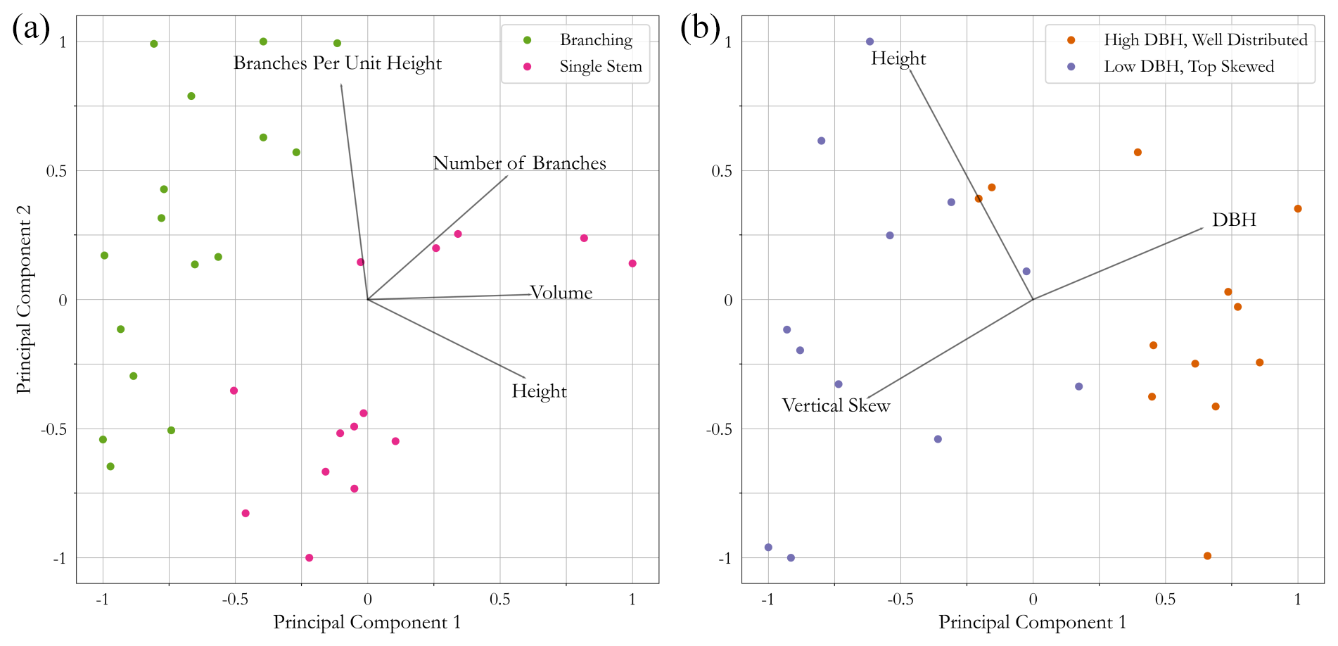
Figure 5 PCA of (a) herbaceous branching and single-stemmed vegetation as well as (b) high-DBH and low-DBH tree functional groups. Lines indicate the direction of each variable that explains variation in the data.

4.1.3 Linking PCA clusters to reach-scale UAV-LS data

Figure 6 shows the results of the seasonal analysis of different variables derived from UAV-LS and UAV-MS imagery for each of the functional group classes. There are clear variables which can separate different functional groups with ease; for example, the height of the canopy is a key indicator between woody, herbaceous, shrub, and grass functional groups. Separating out similar functional groups does appear to be more nuanced. The high-DBH and low-DBH woody functional groups both have very similar values and seasonal patterns of changes in NDVI values as well as in their height. This is unsurprising as the PCA showed height not being a dominant factor in explaining variation, with numerous samples showing crossover. Vertical skew did show group separation, with the samples used for QSM analysis collected in leaf-off conditions. Figure 6 suggests that changes in winter vertical skew are visible between the two tree functional groups, with a smaller amount of crossover as expected. Summer vertical skewness is less informative, likely due to leaf-on conditions affecting full tree reconstruction, with higher variability in results between the sample areas. For example, a tree that has little understorey reconstructed is likely to show little vertical skew compared to one for which below-canopy data are collected.

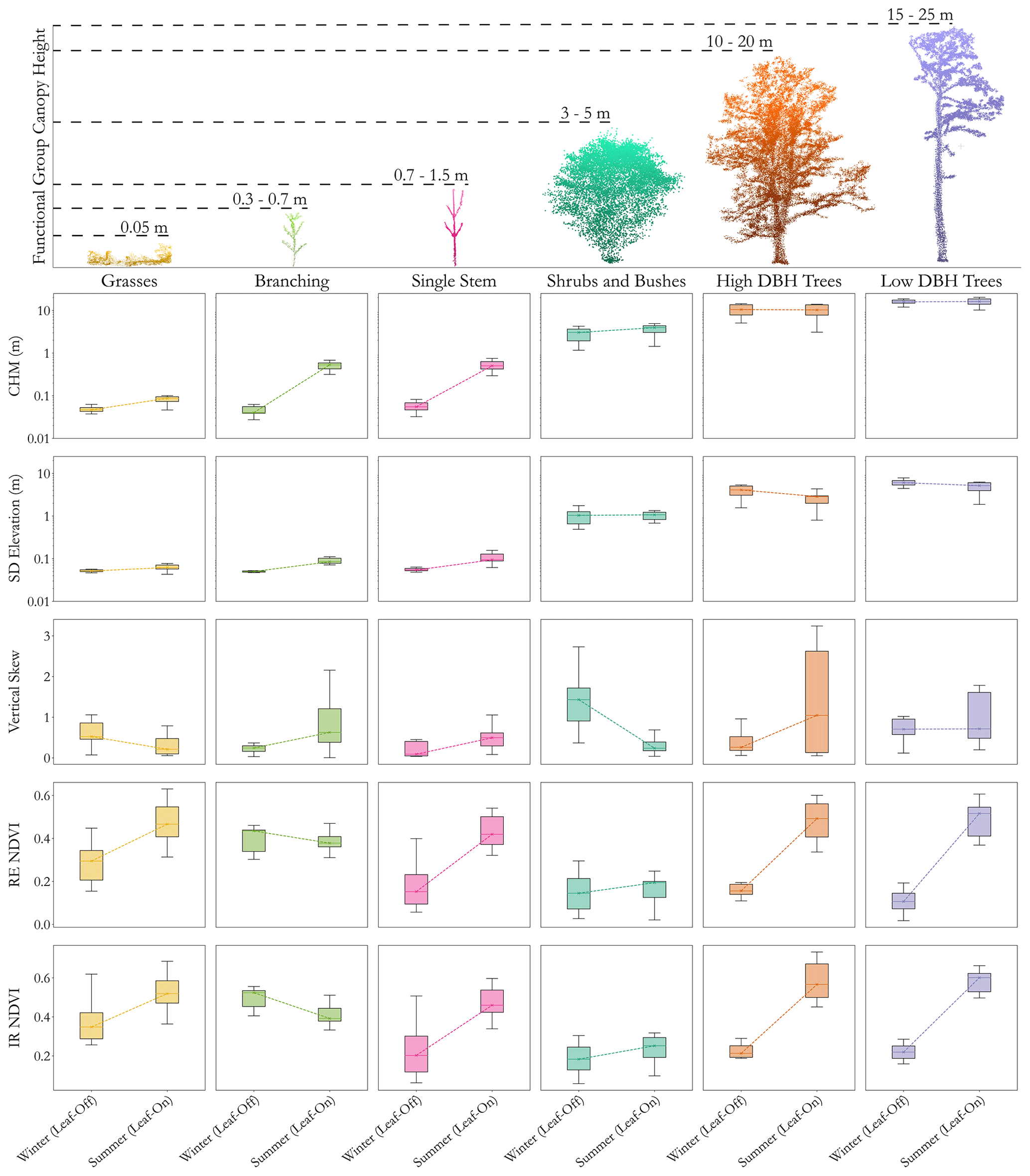
Figure 6 Results of leaf-on and leaf-off analysis (x axis within panels) of different reach-scale metrics (y axis) from UAV-LS and UAV-MS data for each identified plant functional group. The point clouds at the top provide an example of vegetation in each functional group, with canopy height ranges acquired from trait extraction for the four analysed functional groups and from the reach-scale analysis for the remaining grass and shrub functional groups. Box plots indicate the distribution of values derived from the reach-scale data for individual plants. CHM (canopy height model) is given in metres and is plotted in log scale to show the variation for shorter functional groups; IR refers to infrared and RE to red-edge bands in the NDVI calculations. Winter data are from February 2020, and summer data are from July 2020. For plants in the tree groups from the half of the reach not surveyed in July, data from September 2020 were used.

Separating out herbaceous functional groups is also a challenge. CHM values for single-stemmed herbs are more variable and cross over into grasses and multi-branching herbs. However, the mean CHM values are higher, in line with the PCA, and may enable herbaceous group separation. Likewise, the average skew values help to differentiate between classes, but again the variability in the data suggests it is harder to separate by structural content alone. Conversely, spectral data show great promise in differentiating between functional groups. The absolute values between herbaceous functional groups show differences, as do their seasonal patterns, especially when utilising the red-edge band for NDVI calculations.

4.1.4 Creation of seasonal reach-scale functional group maps

The annualised reach-scale classifications (combinations of winter and summer data) based on functional groups and land cover are shown in Fig. 7. Areas surrounding both high- and low-DBH tree groups show a prominence of shrub groups. This may be due to segmented regions during the image classification at the edge of trees having heights similar to those of the shrubs group, possibly leading to a false classification not picked up in the accuracy assessment against the manual classification. Herbaceous groups were predicted in areas typically associated with such vegetation: close to the channel, in side channels which are reactivated over winter, and in mobile areas of the reach where larger vegetation would find it more challenging to establish. The out-of-bag accuracy score when training the random forest classifier with 300 trees was 87.2 %. Figure 8a shows the importance of each band in the classifier, with structural elements proving key in separating functional groups, especially using summer standard deviation of point heights. The near-infrared band and winter standard deviation are the next most important elements, with the remaining individual spectral bands providing a smaller contribution to the classification. The higher importance of the two NDVI layers implies that providing the classifier with analysed image data is more useful than individual bands alone. Likewise, the canopy models alone are less informative than the variation in plant height when detecting functional groups, supporting the use of manipulated rather than simple metrics to help improve classification.

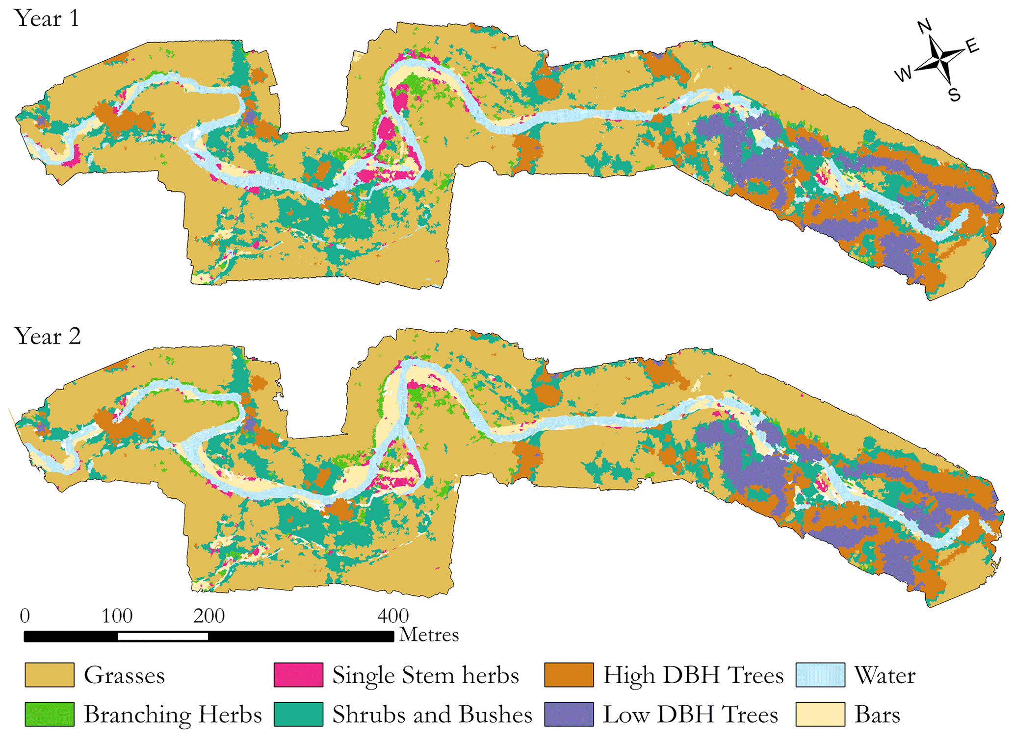
Figure 7 Resulting classification from reach-scale analysis for the areas covered by both UAV-LS and UAV-MS data for year 1 and year 2 of the surveys. Note the changes in channel planform and functional groups through the central section of the reach compared to the relative stability at each end of the reach.

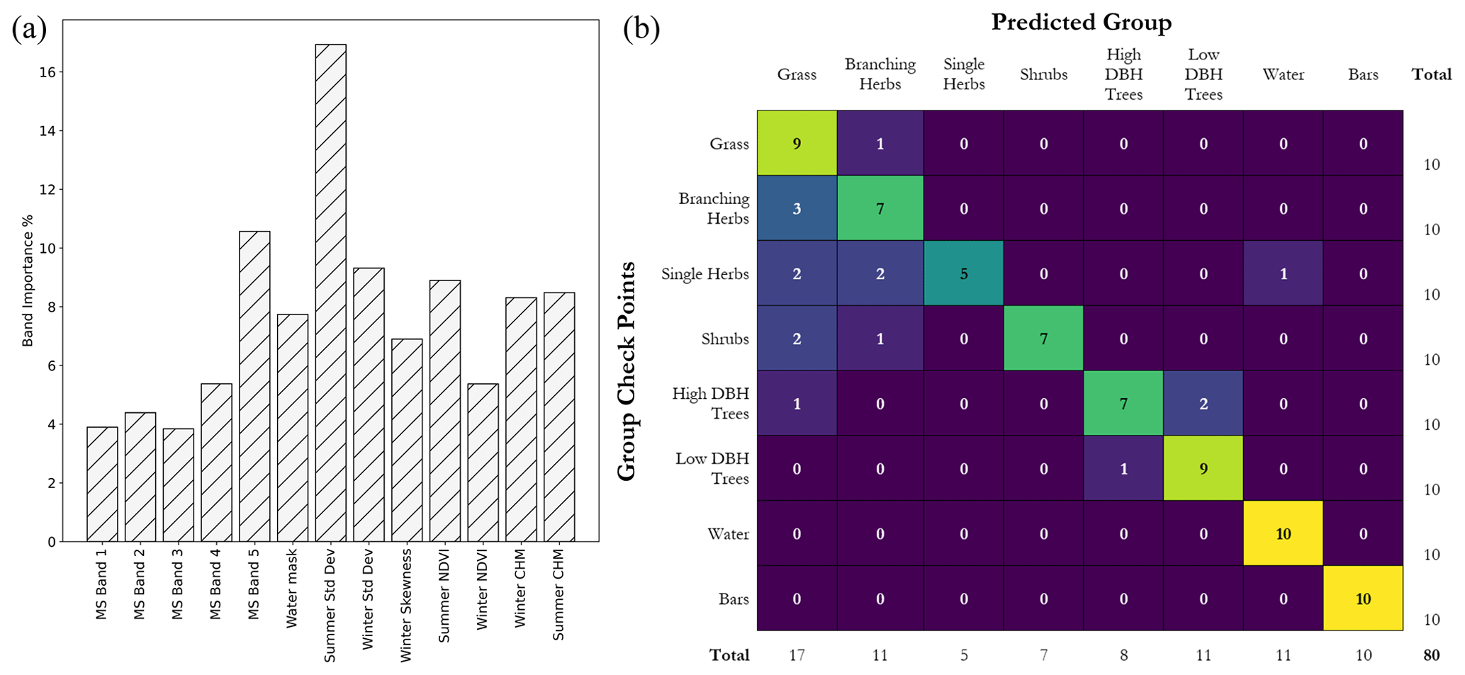
Figure 8 Individual band importance in the final classification (a) and confusion matrix (b) from the accuracy assessment. The band importance represents the contribution of an individual layer to the final classification. The confusion matrix demonstrates for which functional groups the classification struggled, showing an overclassification of grasses and the poor detection of single-stemmed herbs. The overall classification accuracy was 80 %.

The accuracy assessment confusion matrix can be seen in Fig. 8b, comparing the number of manual checkpoints that are correctly and incorrectly predicted by the classifier. The overall model accuracy is 80 %, lower than the out-of-bag prediction. However, this is not surprising as training areas were delineated based on complete structural profiles for the QSM analysis and the total number of samples used for training was small relative to the possible variation across the reach. There was a general overclassification of points within the grass functional group, with only one grass control point incorrectly classed as branching herbs. Branching herbs which are more detectable from imagery and likely to return more laser scan points were classified reasonably well, only being misclassified as grass.

Single-stemmed herbs were relatively poorly classified (50 % accuracy), being misclassified as grass, branching herbs, and water. However, their narrow structure and sparse spacing make them hard to identify from coarser imagery and UAV-LS. This class also exhibited large variations in values when using reach-scale metrics to evaluate functional group samples, overlapping with several other classes. Shrubs were predominantly misclassified as branching herbs and grass; this may be due to the object segmentation not always isolating complete plants or including surrounding ground points, which may have affected the classification. Low-DBH trees with a top vertical skew were classified well by the model, most likely due to their larger heights and winter skew, whereas higher-DBH trees were misclassified as both low-DBH trees and grass. The former is likely due to the difficulty in separating out these two functional groups, which have subtle differences in certain classification layers such as winter skew, and the latter is from surrounding data being included in a segmented object from factors such as shadowing continuing an object outside its true bounds during segmentation. However, of all 20 tree checkpoints, only one was incorrectly classified as a functional group with clearly different traits: a high-DBH tree segment as grass (see Fig. 8b).

4.2 Morphological change

As expected, the majority of morphological change occurs over winter months (Fig. 9) when there are higher flows (Fig. 1). Conversely, over periods of lower flow (see Fig. 1) during the summer both the extent and magnitude of change are reduced. Throughout the first winter period erosion occurs on the outer bank edges with fairly consistent planform evolution throughout the reach. Deposition is evident throughout the entire reach; however, erosion is considerably more dominant than deposition, with just under 3000 m³ of net erosion. The second winter appears to have more localised effects on morphology, with clear channel reshaping through the upper half of the study area. Overall, despite having similar levels of deposition across both winters (∼ 2000 m³) the increase in erosion for the second year led to a greater increase in net erosion (∼ 5000 m³). Both histograms of change within the winter seasons show a dominance in erosion overall. Over both winters, morphological change in the tree group dominated downstream reach has undergone similar levels of change with areas of erosion and deposition influenced by the presence of large vegetation. Both summer periods have a greater degree of stability, with erosion and deposition taking place but in lower magnitudes. This is consistent throughout the reach with no hotspot areas of either deposition or erosion, with deposition shown to be more dominant overall.

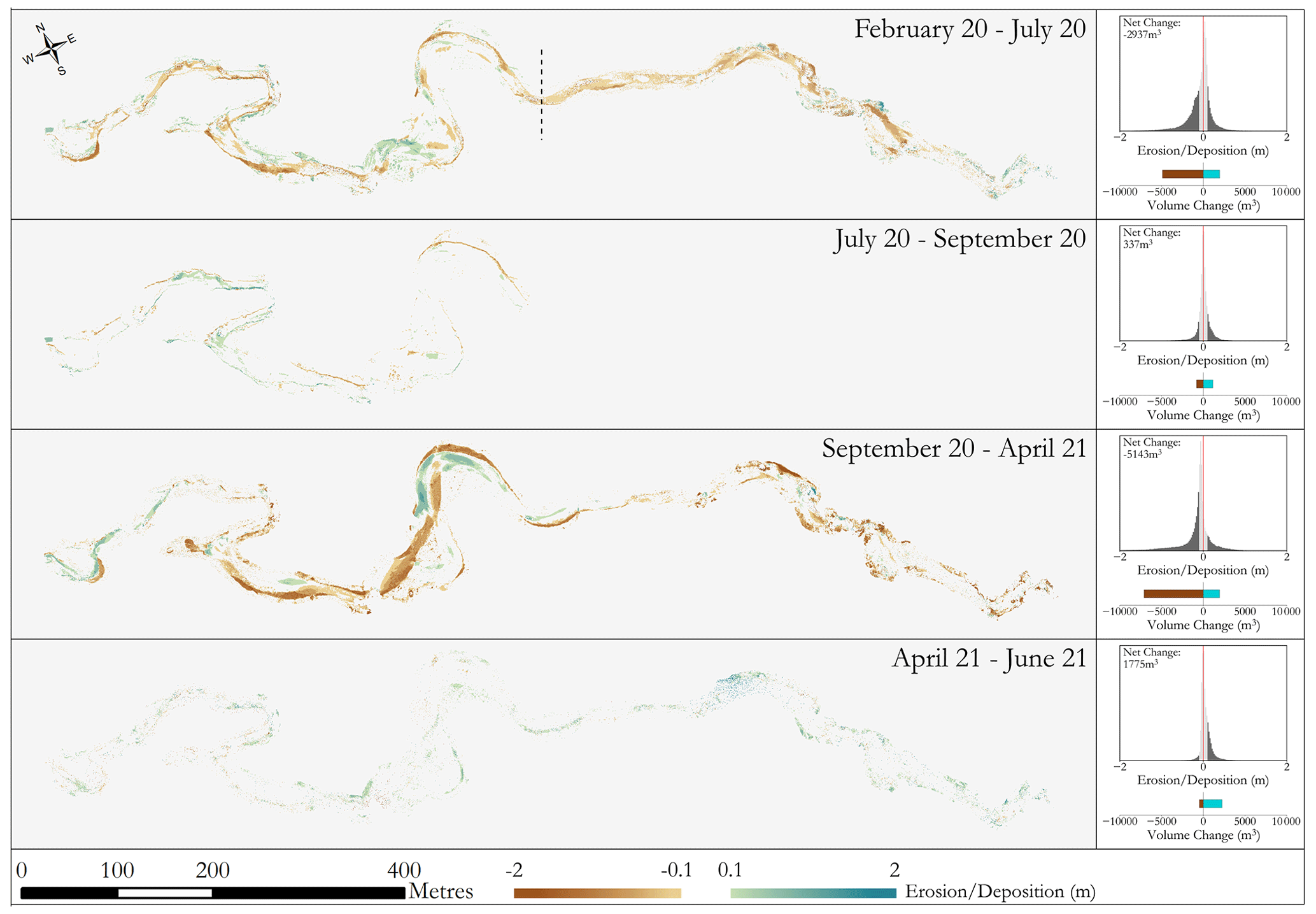
Figure 9 Morphological change throughout the monitoring period, showing the spatial variation in erosion and deposition as well as the net change in sediment. Note that February 20–July 2020 is a composite DEM of difference consisting of comparisons between February and July to the left of the dashed line as well as February and September to the right of it. In July, only half of the survey area was captured. The stability of the reach over summer (July to September) justifies attributing change to the February–July result. Change less than 0.1 m in elevation was not shown as this was deemed below the level of detection of the sensor (see Tomsett and Leyland, 2021a, for accuracy assessment details). The histograms adjacent to each time period show the distribution of magnitude of change, the volume of erosion and deposition over that time period, and the net volume change across the corresponding time periods. Areas of the histogram in light grey depict change below the 0.1 m level of detection.

4.3 Eco-geomorphic interactions

A key benefit of being able to identify the location of different functional groups is the ability to analyse the overall distribution of morphological change within each functional group for each time period (Fig. 10). When assessing the distribution of erosion and deposition between groups across the four time periods, each functional group follows the overall pattern presented in the general morphological analysis, whereby there is a clear dominance of erosion over deposition in winter and a balanced or deposition-dominant signal in the summer periods. Unsurprisingly, erosion dominates in both winters for locations that are classed as water due to lateral migration of the channel. In this case the presence of planform change was the prominent form of morphological change, accounting for a large proportion of the net volume shift, with only grass and high-DBH trees seeing large volumes of net erosion at over 100 m³. In fact, when compared to the changes in the summer, most of the functional groups saw similar magnitudes of change across the two time periods. Compared to winter 2021, however, the net change in volume for areas classified as water was similar, with the remainder of change happening throughout the remaining functional groups and on bars. During this time, there was net deposition on channel bars; however, there are large quantities of both erosion and deposition in this group, in line with the highly active nature of such features. Whilst across all functional groups there is an increase in the net erosion compared with the first winter period, this is exaggerated amongst grasses and shrubs, accounting for 32 % of net erosion. For both cases, these are likely to be the result of channel reactivation during overbank flow removing floodplain sediment. Throughout all of the time periods, no group exhibits a consistent pattern of erosion or deposition, changing based on season and year, making it difficult to identify any direct eco-geomorphic interactions at these scales over these two winter periods. However all groups appear to undergo a dominant erosion signal in the winter followed by an accretion signal in the summer, suggesting that vegetation that can recover or survive peak flows may go on to trap sediment and stabilise the channel and adjacent floodplain.

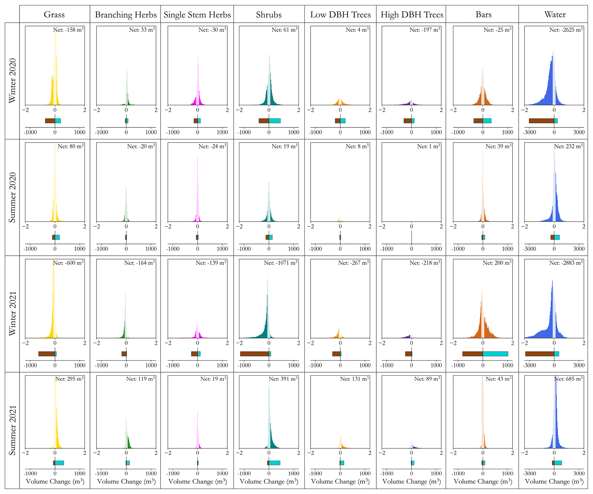
Figure 10 Histograms of morphological change for each classified functional group (x axis) location throughout the reach for each of the time periods studied (y axis). Below each is the volume of erosion and deposition in cubic metres (m³), as well as the net volume change stated in the upper right corners. The transparent elements of the histogram show the change that occurred below the minimum level of detection and was not included in the erosion, deposition, as well as net volume change information. Note the change in x-axis values for the erosion and deposition bars for the water class so as not to subdue the other groups due to the disproportionate amount of change over both winters here.

5 Discussion

5.1 Trait extraction and functional group formation

Current measurements of plant functional traits are still predominantly ground-based; they are therefore limited by on-site access and require extensive sampling (Palmquist et al., 2019; e.g. Diehl et al., 2017a; Hortobágyi et al., 2017; Stromberg and Merritt, 2016). Remote sensing of these traits is therefore a potentially useful way to collect data across larger areas. Although no ground-truth data relating to traits were collected in the field, the assessment of variability in model construction, comparisons between TLS and UAV-LS data, comparisons between UAV-LS data and reconstructed models, and references to wider records in databases and the literature suggest that the methods developed herein were reasonably able to extract physical attributes. This highlights the potential of remote sensing to collect structural trait data for eco-geomorphic research moving forward, especially once trade-offs in terms of time and spatial extent are accounted for.

The use of pre-determined rather than site-specific functional groups was a method employed by Butterfield et al. (2020) on the basis of those outlined in Diehl et al. (2017a). The vegetation in both of these studies was similar, and the application to a temperate UK-based site is challenging because of the complexity and similarities of some plants. When compared to previous studies, the reduction in the number of herbaceous functional groups used herein is due to the data resolution, whereby only two categories could be explicitly detected. The use of a PCA led to the successful separation of functional groups, highlighting metrics which could be used to separate them over larger scales. The influence that different herbaceous vegetation, with variable flexibility and branching structure, has on flow is well studied (e.g. Nepf and Vivoni, 2000; Järvelä, 2004; Sand-Jensen, 2008), and being able to successfully differentiate these two groups highlights the applicability of the survey and trait extraction methods developed in this research. Likewise, the difference in flow conditions between low-DBH trees that are closely packed and less densely packed high-DBH trees may show a resemblance to the influence found at smaller scales on plant density (Järvelä, 2002a; Kim and Stoesser, 2011). The relationship between DBH and vertical skew is not surprising, and as plants could not be easily differentiated by measuring their DBH, using vertical skew provides promising results for upscaling to larger areas, with similar work already being done using vertical distribution to classify forests (Antonarakis et al., 2008; Michałowska and Rapiński, 2021).

UAV-LS data for QSM have been shown to overestimate canopy reconstruction volume (Brede et al., 2019; Dalla Corte et al., 2022), which mirrors the over-complexity demonstrated in the QSM cylinder models (Fig. 3). Extracting traits using remote sensing can improve on ground-based methods for coverage but cannot match the accuracy and interpretive ability of manual in-field measurements yet, as shown by Dalla Corte et al. (2022) for height, DBH, and volume. Moreover, the use of TLS for analysing herbaceous functional groups is highly localised (Lague, 2020), meaning only a small number of samples can be analysed, which may not reflect the full variation in vegetation. The UAV-LS data collected for this study took a significant amount of time to post-process: days for each survey and weeks for the remaining analysis. Yet, algorithms which can extract vegetation and classify large areas are improving in much the same way that SfM methods have developed, making processing times quicker and allowing a greater number of plants to be analysed (e.g. Burt et al., 2019; Krisanski et al., 2021; Yarroudh, 2023; Letard et al., 2023).

Both UAV-LS and TLS also struggle to capture the complex structures of shrubs, with TLS requiring many scans to resolve the structure of enough samples (Boothroyd et al., 2016; Olsoy et al., 2014) and UAV-LS having too low a point density and canopy penetration for such complex branching. However, methods pioneered by Manners et al. (2013) relating vertical profiles from TLS and ALS data may help to overcome this. Similarly, more work is needed to overcome the difficulty in separating out species that appear structurally and spectrally alike, such as woody saplings and herbaceous plants, but which may have different hydraulic impacts. At present, these two different vegetation types could easily be misclassified, and with the likely different interactions with flow and subsequent morphology, not being able to account for these with remote sensing is a limitation. Efforts to further investigate this, possibly using proximity measures to other functional groups or probabilistic rather than categorical classification methods, may help to overcome the issue.

5.2 Reach-scale functional group mapping

The benefits of remote sensing become evident when scaling from individual plants to reach-scale analysis. Finding common features of defined functional groups is more computationally effective than analysing every individual plant throughout the reach at present. Using structural characteristics of the point cloud alongside spectral properties across time allows the leaf-on and leaf-off patterns to enhance functional group classification. It is clear that initial separation between functional group types can be made based on canopy height, although this presents a challenge at the transition between groups. The need for seasonal data is emphasised across functional groups. Herbaceous groups benefit from seasonal patterns in NDVI to complement variation in height, with single-stemmed herbs appearing to show greater seasonal variation. Tree groups, however, require leaf-off data to improve canopy penetration to help separate out each functional group, and as such the timing of data collection will likely impact the effectiveness of this method. Previous work has emphasised the need for seasonal data to improve eco-geomorphic research (Bertoldi et al., 2011; Nallaperuma and Asaeda, 2020), which the results of our research supports. Moreover, for these methods to be implemented at other sites a seasonal approach to surveying is required, as has been undertaken in similar studies (Van Iersel et al., 2018; Souza and Hooke, 2021), yet this presents a limitation for some research.

The accuracy from the random forest classifier is in line with that reported by Butterfield et al. (2020), who used multispectral imagery alone, with most misclassifications happening in functional groups which are similar. This is unsurprising when viewing the uncertainties in functional group properties (Fig. 6), where there is evidence of overlap across multiple attributes for two different groups. Therefore, adjacent groups may be erroneously classified due to having similar spectral and structural characteristics, as well as image segmentation including two groups within one segment. Identifying ways to better segment regions of vegetation may help to improve the overall classification success. However, the outputs here add to the growing body of research using random forests for high-resolution classification approaches (Adelabu and Dube, 2015; Chan and Paelinckx, 2008; Adam and Mutanga, 2009). As the methods here only assign one group for each image segment, elements such as understorey vegetation, which will influence overbank flow, are currently not accounted for.

Despite these limitations, the resulting classification accuracy (Figs. 7 and 8b) shows promise for linking local-scale trait modelling to larger-scale functional group mapping. The spatial distribution of classes throughout the reach aligns with the wider literature, with herbaceous species dominating the active meandering section as these are more adaptable to changing topography and flood conditions, whilst larger woody species which require more stable hydraulic conditions are seen in less active sections of the reach (Kyle and Leishman, 2009; Stromberg and Merritt, 2016; Aguiar et al., 2018). The classification methods herein utilised a mix of structural and spectral data to determine functional group distribution, as opposed to the species identification and subsequent grouping performed by Butterfield et al. (2020). This is important as the same species may display varying traits based on their proximity to the channel (Hortobágyi et al., 2017), and as such using the physical characteristics of plants can be seen as an advantage, yet species identification still plays an important role. However, obtaining secondary data on species traits that are relevant to the area of study can be challenging (see Sect. 4.2.1) and may limit the applicability of trait-based methods to the wider scientific community.

5.3 Eco-geomorphic change

There appears to be more localised evolution in the second winter of surveying, whereas the first winter appears to show a more consistent response throughout the reach. The singular lower peak in water levels for the second winter as opposed to several higher peaks in the first (see Fig. 1c) suggests that priming may be more important for channel movement, whereby a single flow event of lower magnitude can incite a greater resultant planform shift. However, without multiple surveys across the winter, it is hard to determine whether change is predominantly from a single event or multiple events. The response in summer is much smaller in terms of both deposition and erosion, with little morphological change occurring. What change does occur may be from reductions in bank support after high flows leaving banks exposed to collapse (Zhao et al., 2020).

Separating survey data by functional groups does not identify any dominant links between vegetation and morphological change. Yet some of the effects were noticeable, including tree functional groups providing less winter stability than expected based on previous research (Gurnell, 2014; Hortobágyi et al., 2018). However, portions of the western end of the reach are visibly stabilised by vegetation pinning (Figs. 6 and 8), suggesting a mixed effect on morphological change. The lack of any clear pattern could be due to a number of factors. Primarily, the relatively short nature of the study period at 2 years is not necessarily long enough to provide certainty in any feedbacks occurring. In addition, errors in the reconstruction, separation, and classification could propagate through to suggest that the lack of clear pattern is due to the inability to classify functional groups effectively at a reach scale. However, the vegetation reconstruction has proved to be effective within both this study and others (e.g. Brede et al., 2019), producing model attributes in line with previously published values for the same species. The accuracy of the classification was similar to other studies (e.g. Butterfield et al., 2020) and the majority of misclassifications happened between similar groups. Finally, the lack of an obvious link could in part be due to the absence of data linking morphological change and vegetation with relevant flood inundation depths.

To assess the link between vegetation, morphological change, and flood inundation, some simple further analysis was undertaken to explore the possibility of depth-dependent drag being related to morphological change. Based upon the well-established relationship between submerged vegetation frontal area and drag (Nepf and Vivoni, 2000; Järvelä, 2004; Wilson et al., 2006; Gurnell, 2014) we estimated indicative excess drag for each functional group (except grass) at depths of up to 0.1, 0.5, 1, 2, and 4 m for a hypothetical flood. In addition to the previously analysed herbaceous and tree point clouds, 10 additional individual shrub point clouds were extracted to calculate average frontal area. To identify flow depths across the reach, a simple exploratory 2D depth model in Delft3D (Deltares, 2021) was set up to extract hypothetical maximum flood depths across the study area using indicative flows taken from the gauge downstream of the study site for the winter 2021 time period (Fig. 1).

Within the modelled Delft3D water extent, the depth was used to extract the relevant frontal area interacting with the flow. Each of these depth-dependent frontal areas was then used to determine the average excess drag component (F) of a single plant according to

$$\begin{array}{}\text{(1)}& F={\displaystyle \frac{\mathrm{1}}{\mathrm{2}}}{C}_{\mathrm{D}}{A}_{\mathrm{0}}\mathit{\rho }{U}^{\mathrm{2}},\end{array}$$

where C_D is the coefficient of drag, A₀ is the frontal area of the plant facing the flow, ρ is the fluid density, and U is the velocity of the fluid, approximated using Delft3D and a floodplain Manning's n of 0.035 to represent long grass. The excess drag for an individual plant was then transformed into an excess drag per metre squared, being multiplied by the plant density which was calculated using a local maximum filter to identify the top of individual plants, similar to the procedures used to delineate individual trees in dense canopies (Douss and Farah, 2022; Chen et al., 2020). However this approximation does not account for differences in drag caused by variations in the density and distribution of biomass (James et al., 2008; Sand-Jensen, 2008). Drag coefficients were estimated based on morphology and values from the wider literature (see the Supplement). As a result, spatially varying excess drag was approximated across the domain for the winter of 2021 based on an indicative maximum flood extent. This can be used to compare the morphological change to spatially varying estimates of excess drag (Fig. 11), demonstrating the excess drag and aggregated morphological change for each functional group, for each binned flow depth.

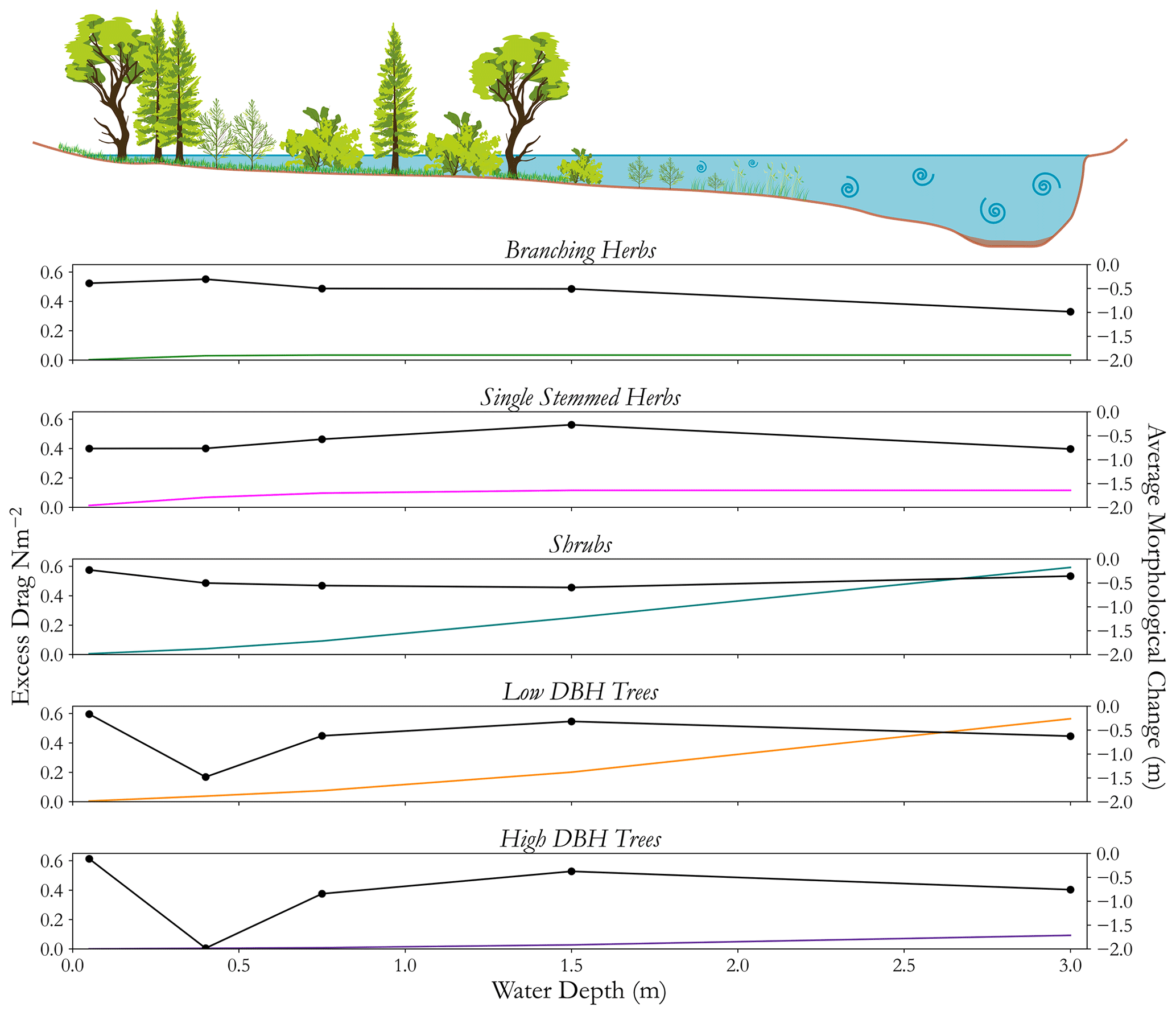
Figure 11 A comparison of how, for each separate functional group, the approximated excess drag (coloured lines, no dots) and morphological response (black line, dotted) change with hypothetical flow depth. The cartoon at the top helps to illustrate how, for different groups, different flow depths result in different proportions of the plant interacting with flow.

All functional groups exhibit an increase in erosion with greater flow depths, as expected due to the increases in shear stress with depth (e.g. Biron et al., 2004; Phillips, 2015). Yet for herbaceous groups, erosion rates are stable or decrease up until the maximum plant heights (see Fig. 6) whereby erosion increases again, suggesting possible moderation due to the vegetation. The remaining three functional groups all see consistently increasing levels of excess drag across flow depths as the plant heights exceed the maximum depth. Shrubs show the most consistent morphological stability, most likely due to their ability to reduce flow speeds and the root structures of larger vegetation providing greater soil cohesion. Both sets of tree groups follow a similar pattern, appearing to accelerate erosion at low flow depths before showing a stabilising effect at greater depth, some of which may be in part due to the poor ability to classify understorey vegetation, missing some of the variability in these areas.

This begins to raise interesting questions around the coupled nature of flow and vegetation, as well as thresholds above which vegetation may begin to dominate in dictating the direction of geomorphic evolution. The exploratory analysis undertaken here begins to investigate this by using structural data across the domain to estimate the influence of vegetation at hypothetical flow depths during an observed flood event, whilst also comparing these to real changes in morphology. Although the drag calculations are averaged for the entire functional group and the morphological signal used is an average, this provides a new and promising avenue of research which could relate individual plant influence on various flood stages and the subsequent morphological response of the channel.

6 Remote sensing of plant functional traits: what next?

One of the key benefits of remote sensing is the ability to quickly capture datasets over scales not possible with ground-based surveying. Although the collection of the data used is fairly straightforward, the subsequent post-processing must be accounted for when considering the routine application of a trait-based approach. Once data have been processed, the success of the classification suggests that functional groups can be classified for other sites that contain similar vegetation in much the same way as previous trait-based research has done (e.g. Butterfield et al., 2020). Moreover, such methods may benefit areas in which ground-based surveying is more challenging, improving the applicability and usability of trait-based methods when compared to traditional taxonomic approaches. However, further assessment comparing ground-based with remotely sensed trait collection is still required.

Combining structural and spectral data provides the opportunity to upscale datasets collected via other platforms, such as high-resolution satellite imagery and ALS datasets. Currently, the main difficulty with trait-based analysis is collecting adequate data over large enough areas. The methodology developed here provides a potential starting point from which a set of tools to classify different hydraulically relevant functional groups across larger areas can be developed. This may overcome some of the scale issues in linking vegetation functional groups to geomorphic change, whereby not enough data to link directions of change with different functional groups have previously been collected.

Future work may also consider how vegetation is represented and how these representations change temporally: for example, the role of vegetation changes from establishment, maturity, and removal over the course of a plant's life. Large trees, for example, transition from stabilising banks during maturity to altering channel flow when removed into the river system (Jeffries et al., 2003; Sear et al., 2010). Likewise, the inclusion of layers such as inundation frequency or flow velocity may improve classification approaches, with different traits being dependent on hydraulic and environmental conditions (Göthe et al., 2017; Corenblit et al., 2015). Moreover, both shrubs and grasses are key elements of UK and other temperate river systems, and remote sensing methods will struggle to capture their complexity due to the sensors' limits of detection, currently relying on species identification from imagery. As such, approaches to improve their integration into the methods presented here (e.g. Manners et al., 2013) are required to be of benefit to wider eco-geomorphic research. Finally, in order to reduce the limitations of combining winter and following summer data, capturing data frequently to enable 4D analysis of how vegetation properties change through time will enable further investigations into eco-geomorphic feedbacks beyond what has been undertaken in this study, particularly focusing on changes occurring during specific geomorphic events.

7 Conclusions

This study has presented a methodological workflow to extract vegetation traits within a river corridor from remotely sensed data before creating functional groups that can be compared to geomorphic change. This presents an important advance in relation to current methods which use species identification from ground surveys or aerial imagery, instead scaling individual plant data to reach-scale classifications. The use of leaf-on and leaf-off surveys enabled the separation of functional groups across the reach, highlighting the benefits of a seasonal approach when utilising remote sensing for vegetation mapping. Despite not identifying discernible directions or magnitudes of geomorphic change between different functional groups, the methods used can still provide a template for future research into eco-geomorphic interactions. Exploratory analysis between depth-related drag and morphological evolution highlighted the potential of using such approaches in the future, where vegetation function and the proximity and interaction with flow can be taken into account.

The potential of UAV-LS for river corridor research is considerable, capturing elements of topography and vegetation simultaneously in ways which are not possible from current SfM approaches alone. In addition, the combination of UAV-LS and SfM data enables greater confidence in the spatial representation of vegetation types and morphological change throughout the river corridor. This is especially pertinent given the seasonal approach employed in this study, where repeat surveying of the reach could be undertaken efficiently without the need for extensive ground surveying. However, this does not replace the need for ground-based methods, with species identification and TLS being used to supplement aerial datasets. These will continue to be required for vegetation groups that are either too small to be captured at the plant scale or too complex for their traits to be captured from UAV platforms. This is an area of research that requires further investigation, allowing for improved integration between remotely sensed and ground-based data. The methods presented herein offer a way in which to address the current gap between individual plant-scale trait analysis and reach-scale functional groups classification, allowing trait-based approaches to be applied to other river reaches of similar scale or greater, enabling greater insight to be gained in relation to eco-geomorphic interactions within the river corridor and beyond.