the Creative Commons Attribution 4.0 License.
the Creative Commons Attribution 4.0 License.
 | 18 Apr 2023
The story of a summit nucleus: hillslope boulders and their effect on erosional patterns and landscape morphology in the Chilean Coastal Cordillera
Dirk Scherler
Renee van Dongen
Hella Wittmann
While landscapes are broadly sculpted by tectonics and climate, on a catchment scale, sediment size can regulate hillslope denudation rates and thereby influence the location of topographic highs and valleys. In this work, we used in situ 10Be cosmogenic radionuclide analysis to measure the denudation rates of bedrock, boulders, and soil in three granitic landscapes with different climates in Chile. We hypothesize that bedrock and boulders affect differential denudation by denuding more slowly than the surrounding soil; the null hypothesis is that no difference exists between soil and boulder or bedrock denudation rates. To evaluate denudation rates, we present a simple model that assesses differential denudation of boulders and the surrounding soil by evaluating boulder protrusion height against a two-stage erosion model and measured 10Be concentrations of boulder tops. We found that hillslope bedrock and boulders consistently denude more slowly than soil in two out of three of our field sites, which have a humid and a semi-arid climate: denudation rates range from ∼5 to 15 m Myr−1 for bedrock and boulders and from ∼8 to 20 m Myr−1 for soil. Furthermore, across a bedrock ridge at the humid site, denudation rates increase with increasing fracture density. At our lower-sloping field sites, boulders and bedrock appear to be similarly immobile based on similar 10Be concentrations. However, in the site with a Mediterranean climate, steeper slopes allow for higher denudation rates for both soil and boulders (∼40–140 m Myr−1), while the bedrock denudation rate remains low (∼22 m Myr−1). Our findings suggest that unfractured bedrock patches and large hillslope boulders affect landscape morphology by inducing differential denudation in lower-sloping landscapes. When occurring long enough, such differential denudation should lead to topographic highs and lows controlled by bedrock exposure and hillslope sediment size, which are both a function of fracture density. We further examined our field sites for fracture control on landscape morphology by comparing fracture, fault, and stream orientations, with the hypothesis that bedrock fracturing leaves bedrock more susceptible to denudation. Similar orientations of fractures, faults, and streams further support the idea that tectonically induced bedrock fracturing guides fluvial incision and accelerates denudation by reducing hillslope sediment size.
Please read the corrigendum first before continuing.
-
Notice on corrigendum
The requested paper has a corresponding corrigendum published. Please read the corrigendum first before downloading the article.
-
Article
(4902 KB)
- Corrigendum
-
Supplement
(702 KB)
-
The requested paper has a corresponding corrigendum published. Please read the corrigendum first before downloading the article.
- Article
(4902 KB) - Full-text XML
- Corrigendum
-
Supplement
(702 KB) - BibTeX
- EndNote


Landscapes on Earth are shaped by tectonic uplift and climate, which dictate erosional and weathering regimes over geologic timescales. When uplift and climate are held constant sufficiently long, fluvial landscapes reach a steady state, in which the slopes of hills and stream channels adjust so that denudation rates match tectonic uplift rates (e.g., Burbank et al., 1996; Kirby and Whipple, 2012). Variations in bedrock strength and the grain size of hillslope sediment, however, exert additional control on the morphology of hills and valleys (e.g., Attal et al., 2015; Glade et al., 2017). Initially, hillslope sediment size is set by lithology and the density of fractures, which are formed due to tectonic and topographic stresses (e.g., Molnar et al., 2007; St. Clair et al., 2015; Roy et al., 2016; Sklar et al., 2017). Near the Earth's surface, water, often carrying biotic acids, infiltrates bedrock fractures and promotes chemical weathering that further reduces sediment size and converts bedrock to regolith (Lebedeva and Brantley, 2017; Hayes et al., 2020). Therefore, long residence times of sediment in the weathering zone (on a million-year timescale) may result in complete disintegration of bedrock and the formation of saprolite and soil, whereas rapid erosion and short residence times can lead to hillslope sediment size limited by fracture spacing (e.g., Attal et al., 2015; Sklar et al., 2017; Roda-Boluda et al., 2018; Verdian et al., 2021). A spectrum between these end-members can also exist within one catchment, especially where variations in lithology, fracture density, or elevation cause spatial differences in the rate and/or extent of weathering (e.g., Sklar et al., 2020). Where weathering does not completely disintegrate the bedrock, boulders, or corestones, can be found embedded in hillslope sediment, with a maximum size set by the spacing of bedrock fractures (Fletcher and Brantley, 2010; Buss et al., 2013; Sklar et al., 2017). Here we focus on the effects of such boulders on differential denudation and landscape morphology on hillslopes with mixed cover of soil, boulders, and bedrock.
Soil-mantled hillslopes are typically considered to be dominated by diffusive processes, for which conceptual models and geomorphic transport laws are relatively well-established (e.g., Dietrich et al., 2003; Perron, 2011). However, these models generally assume uniform hillslope material and do not account for the exhumation of larger boulders through the critical zone. Neely et al. (2019) recently addressed erosion and soil transport on mixed bedrock and soil-covered hillslopes using a nonlinear diffusion model, but assumed the same denudation rate for bedrock and soil. Fletcher and Brantley (2010) modeled the reduction in the size of corestones due to chemical weathering as they are exhumed through the weathering zone, although this model does not consider the corestones' effect on differential erosion. Often, however, bedrock and large boulders protrude above the surrounding soil, indicating that they are eroding more slowly than the soil (Bierman and Caffee, 2002). Indeed, studies have shown that average denudation rates of bedrock outcrops and hillslope boulders are often lower than catchment average and soil denudation rates (e.g., Bierman, 1994; Heimsath et al., 2000, 2001; Granger et al., 2001; Portenga and Bierman, 2011).
Larger boulders require greater forces to be moved, which can be achieved by steepening slopes (Granger et al., 2001; DiBiase et al., 2018; Neely and DiBiase, 2020) or by lengthening residence time until subaerial weathering has decreased their size sufficiently to be transported downslope. During this prolonged residence time, boulders can shield hillslopes from erosion (Glade et al., 2017; Chilton and Spotlia, 2020) and stream channels from incision (Shobe et al., 2016; Thaler and Covington, 2016). In terrain where spatial gradients in bedrock fracture spacing result in spatial gradients of hillslope sediment size, it is thus reasonable to expect the resistance of surface boulders to weathering and transport to retard erosion locally, resulting in spatially differential erosion. Moreover, fractured and therefore weaker bedrock facilitates erosion via both abrasion and plucking by streams (Lamb et al., 2015; Sklar and Dietrich, 2001), and smaller blocks are also more easily transported in fluvial systems (Shobe et al., 2016). Therefore, we would expect rivers to preferentially incise in zones of more intensely fractured rocks (Buss et al., 2013) that align with the orientation of faults (Molnar et al., 2007; Roy et al., 2016).
In this study we provide a new framework for measuring and assessing differential denudation of boulders and the surrounding fine-grained regolith on hillslopes, and we also discuss the extent to which bedrock fracturing affects sediment size, denudation rates, and stream incision. We quantified bedrock, boulder, and soil denudation rates in three different areas along the granitic Coastal Cordillera of Chile with different climates and erosional regimes using in situ cosmogenic 10Be. By developing a simple model to convert 10Be concentrations from boulders into soil and boulder denudation rates, we explored the hypothesis that on a hillslope, boulders affect differential erosion by eroding more slowly than the surrounding soil, with the corresponding null hypothesis that no difference exists between soil and boulder denudation rates. We make the simplifying assumption that soil denudation rates remain constant over the time period that a boulder is exhumed, and over long time periods, denudation rates throughout the landscape vary according to whether boulders or soils are exposed at the surface. Following the logic outlined above, we additionally examined our field sites for signs of fracture control on landscape morphology with the hypothesis that more highly fractured bedrock is more susceptible to denudation and stream incision than intact bedrock.
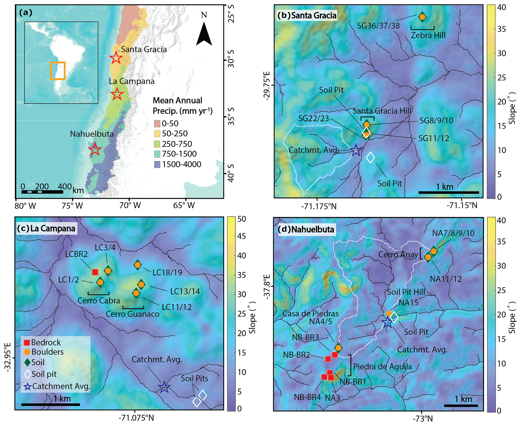
Figure 1Field site locations and features. (a) Map of mean annual precipitation in central Chile, with field sites marked by red stars. Precipitation data from the CR2MET dataset, by the Center for Climate and Resilience Research (CR2) (Boisier et al., 2018), provide an average for the time period 1979–2019. World Terrain Base map sources are Esri, USGS, and NOAA. B-D: slope and hillshade maps from 12.5 m ALOS PALSAR digital elevation models of (b) Santa Gracia (SG; Alaska Satellite Facility Distributed Active Archive Center, 2011b), (c) La Campana (LC; Alaska Satellite Facility Distributed Active Archive Center, 2019), and (d) Nahuelbuta (NA; Alaska Satellite Facility Distributed Active Archive Center, 2011a). Sample locations and sample names are shown, with symbol shape and color indicating the sample type (see legend in c). White outlines delineate the catchments from which the catchment average sample (star) was taken (the catchment from La Campana does not fit within the bounds of the map and is therefore not shown). Black lines indicate streams. Soil pit sample data are from Schaller et al. (2018), and catchment average sample data are from van Dongen et al. (2019).
The Chilean Coastal Cordillera, a series of batholiths in the forearc of the Andean subduction zone, lies along a marked climate gradient with humid conditions in the south and hyper-arid conditions in the north (Fig. 1). The Andean subduction zone, in which the Nazca Plate subducts under the South American Plate, has been active since at least Jurassic times (e.g., Coira et al., 1982). In this study we investigated three field sites along the Coastal Cordillera from south to north: Nahuelbuta National Park (NA) with a humid–temperate climate, La Campana National Park (LC) with a Mediterranean climate, and Private Reserve Santa Gracia (SG) with a semi-arid climate (Fig. 1). NA and SG have more gently sloping hillslopes with a lack of observed landslides, while hillslopes in LC are steeper and landslides have been observed (van Dongen et al., 2019; Terweh et al., 2021). All three sites are underlain by granitoid bedrock (Oeser et al., 2018), none show any signs of former glaciation, and all are located on protected land away from major human influence, such as mines, dams, and large infrastructure. At all three sites, denudation rates from 10Be cosmogenic radionuclide analysis have been reported by van Dongen et al. (2019) (catchment average rates) and Schaller et al. (2018) (soil pits).
NA is located on an uplifted, fault-bounded block (plateau), which is an unusually high part of the Coastal Cordillera with a mean elevation of ∼1300 m a.s.l. (above sea level). Tectonic uplift rates in NA increased from 0.03–0.04 to >0.2 mm yr−1 at 4±1.2 Ma (Glodny et al., 2008), a shift that appears to also be recorded by knickpoints in streams that drain the plateau. All of the measurements in this work are from the plateau (∼9∘ mean slope) above knickpoints (see Fig. S1 in the Supplement). 10Be-derived denudation rates are around 30 m Myr−1 (Schaller et al., 2018; van Dongen et al., 2019), indicating that denudation rates on the NA plateau have not yet adjusted to the higher uplift rates. The main catchment in LC has a mean elevation of 1323 m with a mean slope of 23∘, and regional uplift rates are estimated to be <0.1 mm yr−1 (Melnick, 2016). Van Dongen et al. (2019) reported a catchment average denudation rate of ∼200 m Myr−1 for a sub-catchment in LC, whereas Schaller et al. (2018) reported soil denudation rates of 40–55 m Myr−1. In SG, the mean elevation is 773 m a.s.l., the mean slope is 17.2∘, and uplift rates are <0.1 mm yr−1 (Melnick, 2016). Previously reported 10Be-derived denudation rates are ∼9–16 m Myr−1 (Schaller et al., 2018; van Dongen et al., 2019).
3.1 In situ 10Be analysis
3.1.1 Sample collection
We collected samples for cosmogenic 10Be analysis from bedrock, boulders, and soil to estimate denudation rates at our field sites, targeting hillslopes near previously collected catchment average and soil pit samples from van Dongen et al. (2019) and Schaller et al. (2018). All sample locations are shown in Fig. 1. Bedrock samples were taken using a hammer and chisel from an area of up to ∼20 m × 20 m (on ridge tops or hillslopes) and consist of an amalgamation of at least 10 chips (∼25 cm2 and <2 cm thick), with which we aim to obtain representative mean values of denudation rates that are potentially variable due to episodic erosion by spalling rock chips (Small et al., 1997). Similarly, for boulder samples, one chip was taken from the top of each of at least 10 similarly sized boulders and amalgamated for an area of up to ∼40 m × 40 m, depending on boulder abundance. Topsoil samples were also collected by amalgamation in the area surrounding the sampled boulders. In places with many variously sized boulders, we collected samples from different protrusion heights (∼1 m tall boulders, ∼0.5 m tall boulders, etc.). Each sampled boulder was measured along the a, b, and c axes, as far as discernible (see Table 1). We also measured the protrusion height of each boulder from the center of the top of the boulder to the ground. Each protrusion height value in Table 1 consists of an average of at least 10 boulders of similar protrusion heights that we sampled for one amalgamated sample. Boulders on sloping surfaces typically show varying protrusion heights, with higher values downslope and lower values upslope. In such cases, we measured protrusion at the sides of boulders. Occasionally, we observed that upslope protrusion was further reduced by sediment trapping upslope of boulders. We targeted boulders that appear to be in situ (essentially, exhumed corestones) based on the observation that they are tightly imbedded in the ground. We acknowledge that it is possible that some of the larger sampled boulders are connected to bedrock roots and that it is also possible that some boulders are not in situ, despite our best efforts.
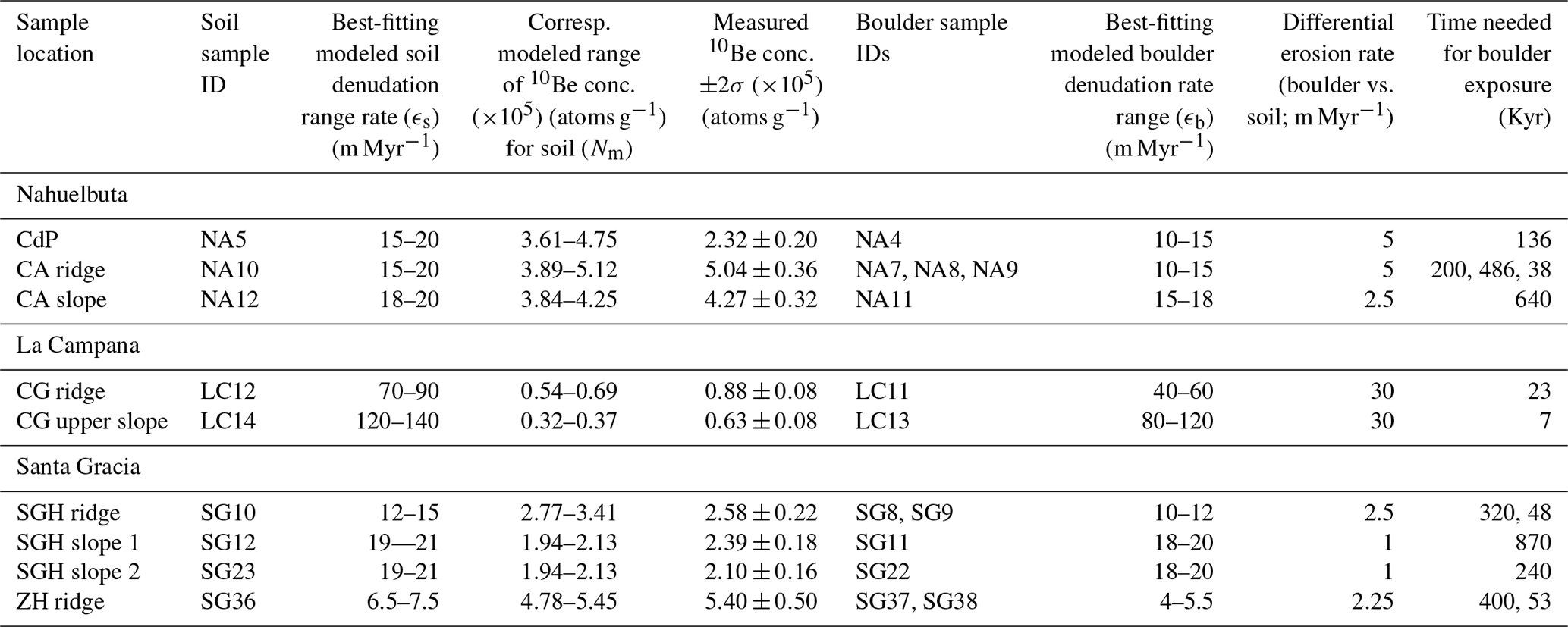
Table 110Be cosmogenic nuclide sample data.
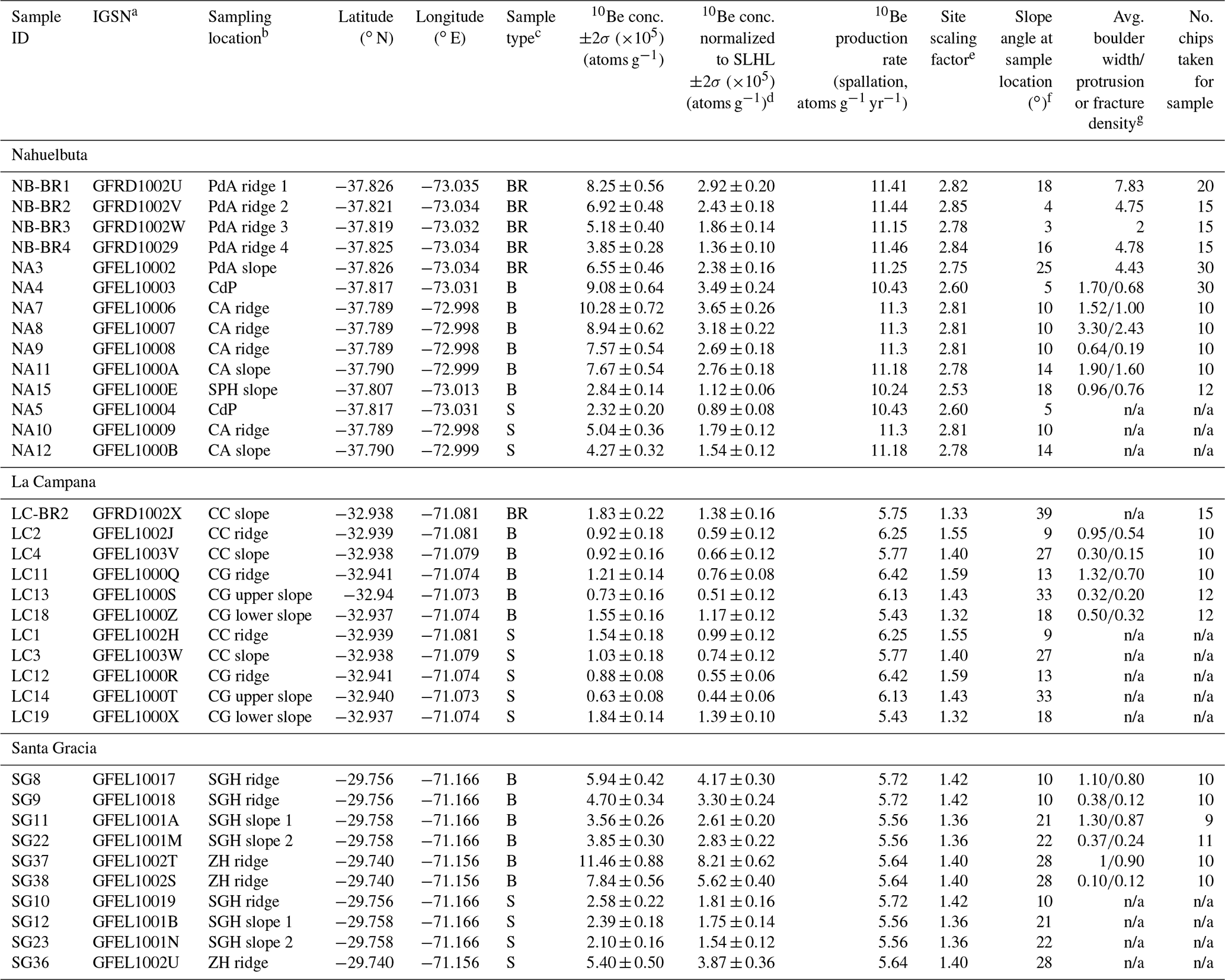
a Open-access metadata: http://igsn.org/ (last access: 1 January 2023). b Sample locations. PdA: Piedra de Aguila, CdP: Casa de Piedas, CA: Cerro Anay, SPH: Soil Pit Hill, CC: Cerro Cabra, CG: Cerro Guanaco, SGH: Santa Gracia Hill, ZH: Zebra Hill. c Sample type abbreviations. BR: bedrock, B: boulders, S: soil. d Concentrations were normalized to SLHL (sea level high latitude) by dividing the measured concentrations with the site's scaling factor. e Time-constant spallation production rate scaling scheme of Lal (1991) and Stone (2000) (“St” in Balco et al., 2008), calculated taking topographic shielding into account; f local hillslope angles were calculated using a 12.5 m DEM and an eight-connected neighborhood method. g Fracture density for bedrock (in meters) and width and protrusion measurements (in meters) for boulders. Values are averages of >10 measurements per sample site. The notation “n/a” stands for not applicable.
In NA, we collected five bedrock samples from an area called Piedra de Aguila from outcrops with different fracture densities and measured fracture spacing (47 measurements) by stringing a measuring tape along the bedrock surface and measuring the distance between fractures that were at least 1 mm wide and fracture orientations (41 measurements) using a Brunton compass (Fig. 2a1 and a2). We further collected six boulder samples and three soil samples from the ridge and hillslope of Cerro Anay (Fig. 2a3), an area called Casa de Piedras, and a hillslope near the soil pits that were sampled by Schaller et al. (2018). We measured the dimensions of all boulders from which we took a sample chip (141 boulders). In LC and SG, we were not able to collect samples at variably fractured bedrock outcrops due to rarely exposed bedrock. In LC, we took one bedrock sample, two boulder samples, and two soil samples from the ridge and slope of Cerro Cabra (Fig. 2b1), as well as three boulder samples and three soil samples from the ridge, upper slope, and lower slope of Cerro Guanaco (Fig. 2b3). In SG, we took four boulder samples and three soil samples from the ridge and slope of Santa Gracia Hill, which also hosts the soil pits of Schaller et al. (2018) (Fig. 2c2 and c3), as well as two boulder samples and one soil sample from the ridge of Zebra Hill (Fig. 2c1).
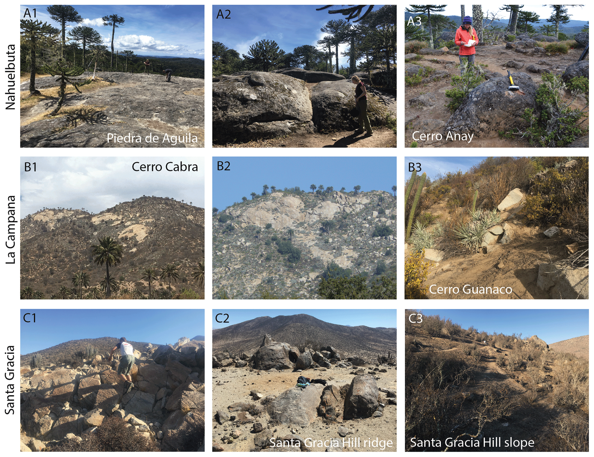
Figure 2Field photos showing the various surfaces sampled, including bedrock, boulders, and soil. Figure panels are grouped by field site. (a) Nahuelbuta, (a1) bedrock (sample NB-BR1). (a2) Fractured bedrock, in transition between unfractured bedrock and boulders (sample NB-BR2). (a3) Smaller boulders surrounded by soil (sample NA7). (b) La Campana, (b1) bedrock (sample LC-BR2). (b2) Bedrock transitioning to large boulders and soil. (b3) Boulders and soil on a hillside (samples LC13 and LC14). (c) Santa Gracia, (c1) boulders on Zebra Hill delineated by fractures. (c2) Large boulders on the ridge of Santa Gracia Hill (sample SG8). (c3) Soil with minimal boulders on the slope of Santa Gracia Hill (samples SG22 and SG23).
3.1.2 Analytical methods
We dried, crushed, and sieved amalgamated bedrock and boulder samples for quartz mineral separation, and we dried and sieved soils, each to 250–500 µm particle size or to 250–1000 µm if the 250–500 µm sample amount was not sufficient. We used standard physical and chemical separation methods to isolate ∼20 g of pure quartz from each sample. After spiking each sample with 150 µg of 9Be carrier and dissolving the quartz in concentrated hydrofluoric acid, we extracted Be following protocols adapted from von Blanckenburg et al. (2004). ratios were measured by accelerator mass spectrometry at the University of Cologne, Germany (Dewald et al., 2013). Sample ratios were normalized to standards KN01-6-2 and KN01-5-3 with ratios of and , respectively. Final 10Be concentrations were corrected by process blanks with an average ratio of .
3.1.3 Denudation rate calculations
In order to calculate denudation rates from the measured 10Be concentrations, we evaluated bedrock, boulder, and soil samples differently. Bedrock samples present the simplest case, in which we assumed steady-state erosion and calculated bedrock denudation rates (ϵbr) using the CRONUS online calculator v2.3 (Balco et al., 2008). The steady-state assumption is based on our amalgamated sampling and follows the results of Small et al. (1997), who showed that an amalgamation of several individual bedrock samples is a reasonable approximation of the long-term average denudation rate in episodically eroding settings.
Boulder and soil samples require a more nuanced assessment. Boulders protrude above the ground surface, which implies that the lowering of the ground surface (i.e., the soil denudation rate, ϵs) is faster than the lowering of the boulder's surfaces (i.e., the boulder denudation rate, ϵb) (Fig. 3). Thus, even while they are buried and covered by soil (or saprolite), boulders are exposed to cosmic rays for a significant amount of time prior to breaching the surface (Fig. 3a). We refer to this time span as phase 1. When boulders breach the surface, they should have a concentration similar to that of the surrounding soil (Fig. 3b). As boulders are exposed during phase 2, nuclide production and decay continues, but it takes time for the boulder surfaces to attain a 10Be concentration that is in equilibrium with the slower boulder denudation rate. Thus, we expect that the measured concentrations from the tops of boulders are combinations of the two different phases in which 10Be is accumulated at different rates (first a rate corresponding to the soil denudation rate and, after exhumation, a rate corresponding to the boulder denudation rate). Converting the 10Be concentrations of soil samples collected from around the boulders to a denudation rate also requires a special approach, as these samples include an unknown number of grains eroded off boulders, which ought to increase the 10Be concentration due to the slower denudation rate of boulders compared to soil.
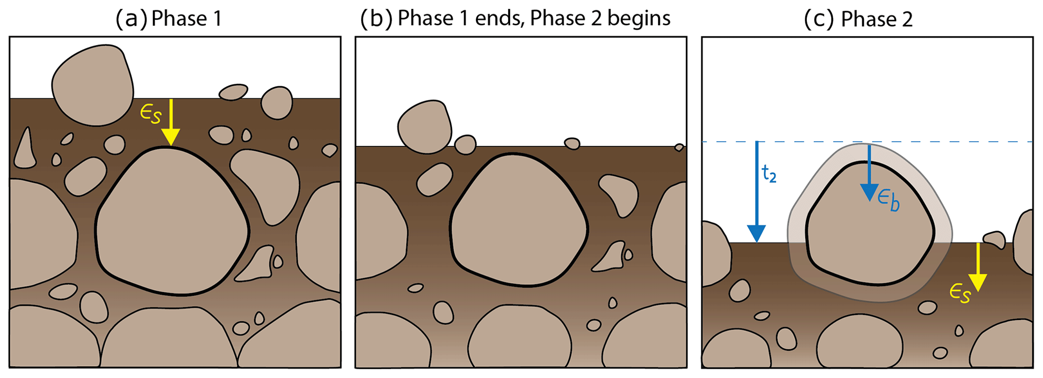
Figure 3Schematic image showing the process of boulder exhumation. (a) Overview of the setting: a mixed soil- and bedrock-covered hillslope where sediment size decreases with decreasing fracture spacing. (b) During phase 1, the boulder is buried and accumulates nuclides at a rate governed by the soil denudation rate, ϵs. (c) Phase 1 ends when the boulder breaches the soil surface. (d) During phase 2, the boulder itself is eroding at a rate of ϵb, and the surrounding soil continues to denude at a rate of ϵs. Phase 2 lasts for a time period t2 that ends with our sampling.
Because of the above complications, we used an approach to estimate the soil and boulder denudation rates that considers the measured boulder protrusion heights and their measured 10Be concentrations. We modeled 10Be concentrations (Nmodeled, atoms g−1) by approximating the production rate profile with a combination of several exponential functions (e.g., Braucher et al., 2011) during the two different phases:
where i indicates different terms for the production by spallation, fast muons, and negative muons; Pi(0) represents the site-specific 10Be surface production rates (atoms g−1 yr−1) for the different production pathways (Table 1); λ is the 10Be decay constant (; ϵb is the boulder denudation rate (cm yr−1); and Λi is the attenuation length scale (160 g cm−2 for spallation, 4320 g cm−2 for fast muons, and 1500 g cm−2 for negative muons, respectively; Braucher et al., 2011). ρ is the bedrock and boulder density, and here we use a value of 2.6 g cm−3 for all samples; we discuss the impact of density changes in Sect. 5.1. Surface production rates by spallation are based on an SLHL (sea level high latitude) reference production rate of 4.01 atoms g−1 yr−1 (Borchers et al., 2016) and the time-constant spallation production rate scaling scheme of Lal (1991) and Stone (2000) (“St” in Balco et al., 2008). Surface production rates by both fast and negative muons were obtained using the MATLAB function “P_mu_total.m” of Balco et al. (2008). Topographic shielding at each sampling site was calculated with the function “toposhielding.m” of the TopoToolbox v2 (Schwanghart and Scherler, 2014) and 12.5 m resolution ALOS PALSAR-derived digital elevation models (DEMs) from the Alaska Satellite Facility.
In Eq. (1), the first term represents phase 1 and the second term represents phase 2, with t2 being the exposure time of the boulder, calculated from the height of the boulder (z) divided by the difference between the soil denudation rate and the boulder denudation rate:
For each sample and associated average boulder protrusion height, we modeled 10Be concentrations with Eq. (1) for different combinations of soil and boulder denudation rates that we allowed to vary between 5 and 50 m Myr−1 (NA), between 3 and 50 m Myr−1 (SG), and between 10 and 300 m Myr−1 (LC), guided by previously published denudation rate estimates (Schaller et al., 2018; van Dongen et al., 2019). We consider permissible denudation rates to be those for which the difference between the modeled and observed 10Be concentrations is less than the measured 2σ concentration uncertainty.
This idealized model rests on several assumptions: (1) the landscapes are in a long-term steady state wherein denudation is locally variable as boulders and bedrock are exhumed in different locations, but this variation is around a long-term stable average; (2) soil denudation rates remain steady over the course of boulder exhumation; (3) boulders are in situ and have not rolled downhill; (4) boulders have not been intermittently shielded during their exhumation; and (5) soil density is inconsequential and can be assigned the same value as bedrock. Assumption 3 has a higher chance of being violated on steep slopes or where boulders are tall, and assumption 4 is more likely violated where boulders are densely clustered. These assumptions are discussed in more detail in Sect. 5.1.
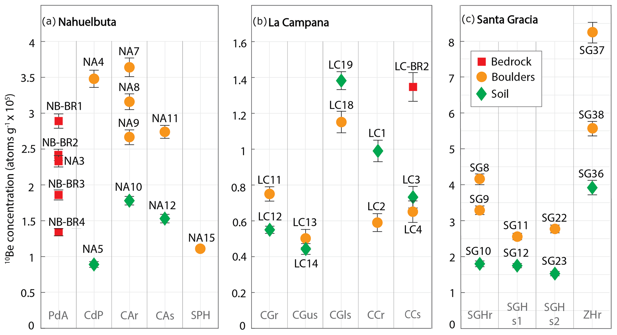
Figure 4Measured 10Be concentrations normalized to reference production rate at sea level high latitude for (a) Nahuelbuta, (b) La Campana, and (c) Santa Gracia; note the different scales of y axes. The x axes are not numerical but rather show the sampling locations, also reported in Table 1. Labels next to data points provide sample IDs, also reported in Table 1. Gray labels at the bottom of panels are the sample locations. PdA: Piedra de Aguila, CdP: Casa de Piedas, CAr: Cerro Anay ridge, CAs: Cerro Anay slope, SPH: Soil Pit Hill, CGr: Cerro Guanaco ridge, CGus: Cerro Guanaco upper slope, CGls: Cerro Guanaco lower slope, CCr: Cerro Cabra ridge, CCs: Cerro Cabra slope, SGHr: Santa Gracia Hill ridge, SGHs1: Santa Gracia Hill slope 1, SGHs2: Santa Gracia Hill slope 2, ZHr: Zebra Hill ridge.
3.2 Topographic analysis
To test if stream orientations at our field sites follow fault orientations, we analyzed the orientations of streams using 1 m resolution lidar DEMs (Kügler et al., 2022). Within each DEM, we first calculated stream networks based on flow accumulation area thresholds of 104, 105, and 106 m2. The lowest threshold was determined based on the occurrence of incised channels visible in the DEMs. We then used the TopoToolbox function “orientation” with a default smoothing factor (K) of 100 to obtain the orientation of each node in the stream network. Fractures in the field can only be seen where there are bedrock outcrops, which are generally scarce. Therefore, we decided to refer to the orientation of faults, as depicted in geological maps, with the assumption of similar orientation (Krone et al., 2021; Rodriguez Padilla et al., 2022). To obtain the orientation of mapped faults, we extracted faults within ∼50 km of each sampling site from a 1:1 000 000 scale geological map from Chile's National Geology and Mining Service in ArcGIS (SERNAGEOMIN, 2003). Fault orientations were measured for straight fault segments with a length of 100 m. Because we are only interested in the strike of streams and faults, all orientations lie between 0 and 180∘. For displaying purposes in rose diagrams, we mirrored these values around the diagram origin by duplicating values and adding 180∘.
4.1 10Be concentrations
Measured 10Be concentrations span a wide range of values and are generally lowest in LC and higher in NA and SG (Table 1). Within NA, we observe the lowest averaged 10Be concentrations (normalized to SLHL) for soil samples ( atoms g−1), followed by bedrock samples ( atoms g−1) and boulder samples ( atoms g−1) (Fig. 4a). In NA at Piedra de Aguila, where we were able to measure fracture spacing in areas with exposed bedrock, the 10Be concentrations of samples from fractured bedrock decrease with increasing fracture density (Fig. 5a). One boulder sample from the slope of Soil Pit Hill stands out with a concentration that is lower than most soil samples. Similar but slightly higher average values than in NA are attained in SG, with soil samples ( atoms g−1) being lower than boulder samples ( atoms g−1) (Fig. 4c). Only in LC are the differences between averaged soil ( atoms g−1) and boulder samples ( atoms g−1) small and, with 2σ error, within uncertainties (Fig. 4b). In addition, at three out of five sampling locations in LC, boulders have lower concentrations than adjacent soil samples, which is inconsistent with the assumption that ϵs<ϵb (see Sect. 3.1.3). However, our single bedrock sample from LC has a higher concentration of atoms g−1. In NA and SG, boulder samples from slope locations have lower average 10Be concentrations compared to boulder samples from ridge locations. Again, in LC this pattern does not hold. Finally, we do not observe a significant trend between 10Be concentration and protrusion height (Fig. 5d); however, there is a relationship between protrusion height and slope for LC (Fig. 5e).
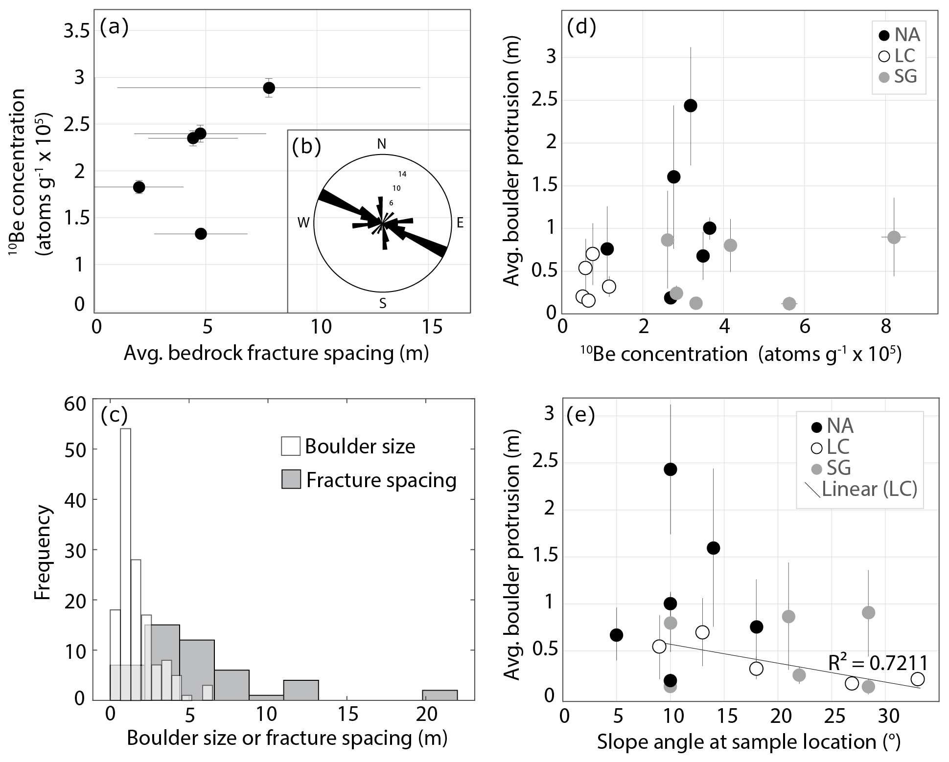
Figure 5(a) Average bedrock fracture spacing (NA only), plotted against measured 10Be concentrations normalized to the reference production rate at sea level high latitude. Error bars represent the standard deviation of all fracture spacing measurements for each location. (b) Rose diagram showing bedrock fracture orientations measured in the field in NA (same fractures as panel a). (c) Measurements of individual fracture spacing and individual boulder sizes, with boulder size being the average of the x and y axes of each boulder and the z axis the protrusion height. (d) Average boulder protrusion height plotted against measured 10Be concentrations normalized to the reference production rate at sea level high latitude for each field site. Error bars represent the standard deviation of all boulder protrusion height measurements for each location. (e) Average boulder protrusion height plotted against hillslope angle. A linear regression model is fit through LC data points.
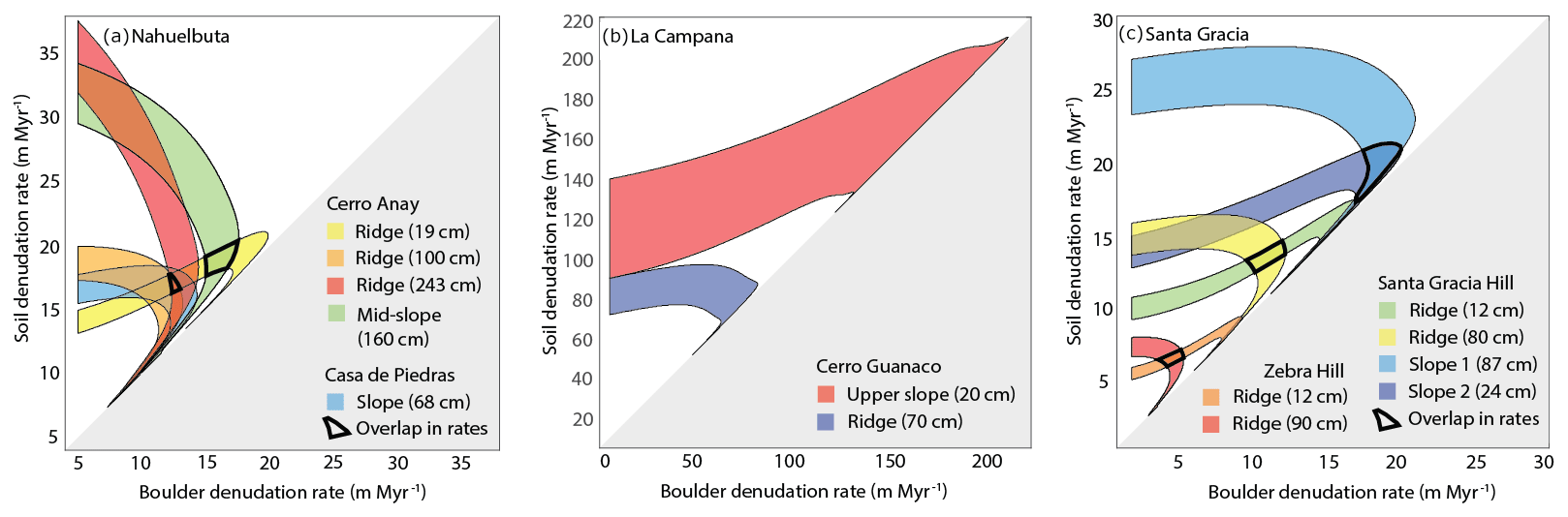
Figure 6Range of best-fitting combinations of modeled soil and boulder denudation rates in (a) Nahuelbuta, (b) La Campana, and (c) Santa Gracia according to Eq. (1). Each color band corresponds to an amalgamated boulder sample, listed in the legend along with the average protrusion height of the boulders. Areas where best-fitting denudation rates overlap for samples from the same location are highlighted by a black outline. The gray areas are forbidden fields, as by assumption, boulder denudation rates have to be lower than soil denudation rates; otherwise, there would be no boulder protruding above the soil surface.
4.2 Bedrock, boulder, and soil denudation rates
Bedrock denudation rates in NA range from 8.53±0.60 m Myr−1 to 18.64±1.40 m Myr−1, and the LC bedrock sample yielded a denudation rate of 22.28±2.62 m Myr−1. We modeled boulder (ϵs) and soil denudation rates (ϵs) using the approach described in Sect. 3.1.3 for all boulder samples that have higher concentrations than the adjacent soil concentrations. We address locations where 10Be concentrations are higher in soil compared to boulder samples in the Discussion section (three locations in LC and one in NA). In contrast to the bedrock denudation rates, modeled boulder and soil denudation rates have no unique solution, and their ranges of possible denudation rates are more complex (Fig. 6). The ranges of denudation rates, illustrated by the curves in Fig. 6, are comprised of values for which the differences between the measured and modeled 10Be concentrations are less than the measured 2σ 10Be concentration uncertainty, with modeled 10Be concentrations based on Eq. (1). Each colored band represents one amalgamated boulder sample (such as 1 m protruding boulders from the ridge of Cerro Anay). The x axis shows the range of modeled boulder denudation rates, and the y axis shows the range of modeled soil denudation rates. However, not every combination within the range plotted in Fig. 6 is plausible. For example, the part of the colored bands in Fig. 6 that is close to the 1:1 line (edge of the gray area) exists because at very low differential denudation rates (differences between soil and boulder denudation rates), phase 2 gets very long so that the boulder denudation rate dominates the resulting concentration and approaches the value one would obtain when neglecting the first term on the right side in Eq. (1). We argue that differential denudation rates of less than ∼1 m Myr−1 are highly unlikely, as it would take ∼1 Myr to exhume a boulder of only 1 m in height above the soil, while simultaneously eroding many times more soil and boulder material.
In NA, permissible modeled soil denudation rates range from ∼13 to 37 m Myr−1 and permissible modeled boulder denudation rates range from ∼5 to 20 m Myr−1 (Fig. 6a). Three samples that were taken from the same ridge at Cerro Anay (Figs. 2a3 and 4a) all overlap in denudation rate despite varying protrusion heights. These samples also overlap with a sample from Casa de Piedras and together indicate a rather narrow range of soil and boulder denudation rates of ∼15–20 and ∼10–15 m Myr−1, respectively. Only the mid-slope sample from Cerro Anay has higher modeled soil and boulder denudation rates. In LC, modeled boulder and soil denudation rates that are consistent with the measured 10Be concentrations extend to much higher values compared to the other field sites (40–140 m Myr−1; Fig. 6b) and the two solutions do not overlap. In SG, permissible modeled denudation rates are similar in magnitude to results from NA (Fig. 6c); soil denudation rates range from ∼7 to 28 m Myr−1 and boulder denudation rates range from ∼4 to 23 m Myr−1. Samples taken from the ridge of Santa Gracia Hill (Figs. 2c2 and 4c) have permissible modeled soil and boulder denudation rates that overlap at values of ∼12–15 and ∼10–12 m Myr−1, respectively, whereas samples from the ridge of Zebra Hill overlap at ∼4–5.5 m Myr−1 for boulders and ∼6.5–7.5 m Myr−1 for soil. Samples from the slope of Santa Gracia Hill have higher modeled soil denudation rates, when considering very low differential denudation rates unlikely. We further discuss the most plausible ranges of denudation rates in Sect. 5.1 and 5.2.
4.3 Fault and stream orientations
Fault orientations at our field sites, based on straight segments of 100 m (8731 segments for SG, 6572 segments for LC, and 6214 segments for NA), generally have at least one dominant orientation that aligns with stream orientations (Fig. 7). Stream orientations depend on the flow accumulation threshold: at smaller thresholds (104 m2), abundant small streams yield a wide distribution of orientations that seems to reflect the shape of the catchment as a whole. At a high flow accumulation threshold (106 m2), the derived stream networks comprise only the largest channels and their orientation is strongly controlled by the orientation and tilt of the drainage basin. This can be seen clearly in NA, where the east–west-oriented trunk stream is weighted heavily. In SG, faults and stream orientations match each other well, both trending north–south. In LC and NA, one of two regional fault orientations match stream orientations, and faults closest to the field sites more closely match dominant stream orientations (red faults in Fig. 7). Specifically, in LC, the dominant orientations for the regional faults are roughly northeast and secondarily northwest, whereas streams are generally oriented northwest. In NA, faults generally have east–west and northwest–southeast orientations, and streams with an accumulation threshold above 104 follow an east–west orientation. Fracture orientations measured in the field (in NA) also generally agree with the larger fault and stream orientations, with mostly west-northwest–east-southeast orientations (Fig. 5b). Our fracture spacing measurements are mostly in the range of 2–15 m (Fig. 5a), while our boulder width measurements are generally smaller (0–5 m). When plotted together, the distribution of boulder sizes sits at the left tail of the distribution of the fracture spacing measurements (Fig. 5c).
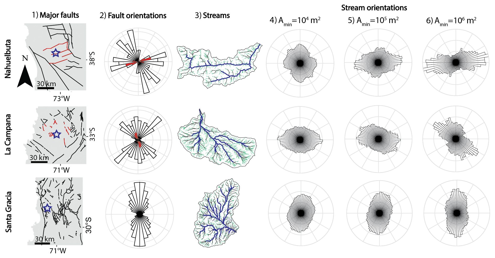
Figure 7Rose diagram plots and maps showing fault and stream orientations for Nahuelbuta (top row panels), La Campana (middle row panels), and Santa Gracia (bottom row panels). For each field site, the columns show the following from left to right: (1) major faults digitized from a geological map (SERNAGEOMIN, 2003) within ∼50 km (black) and ∼25 km (red, NA and LC only) of the sampling site (blue star); (2) rose diagram of fault orientations from the maps in column 1, constructed using 100 m long, straight fault segments and 36 bins, with orientations of faults < 25 km from NA and LC in red; (3) a map of the studied catchments and the drainage network, with green, black, and blue streams indicating minimum upstream areas (Amin) of 104, 105, and 106 m2, respectively, derived from 1 m resolution lidar DEMs (Kügler et al., 2022); (4–6) rose diagrams (72 bins) of stream orientations for different Amin. All maps and rose diagrams are oriented with the top being north.
5.1 Deciphering the denudation rates of boulders and soil
Our model results show that no unique combination of soil and boulder denudation rates exists for any particular site (Fig. 6). What, then, are the most plausible combinations of boulder and soil denudation rates? The answer depends on the characteristic exhumation histories of the boulders and events that could have influenced the accumulation of 10Be during the course of exhumation. In order to narrow down the ranges of denudation rates for boulders and soils investigated in this study, we address our model assumptions and complicating factors, such as shielding and toppling of boulders, and compare measured and modeled 10Be concentrations of soils to each other.
Our model rests on five main assumptions outlined at the end of Sect. 3.1.3. The first is that the long-term steady state of the landscape is difficult to assess; however, the lack of knickpoints above our sampling locations (Fig. S1) suggests this to be reasonable. With our dataset, it is also difficult to assess assumption 2 regarding whether soil denudation rates were steady or variable throughout boulder exhumation; however, we speculate on this possibility below. Assumptions 3 and 4, regarding boulder mobility and shielding, are discussed in depth in the next section. Assumption 5 is that the density of soil can be treated like the density of boulders and bedrock. Although the density of soil and saprolite layers is in reality lower, we assume a steady thickness of these layers through time, which means that the lowering of the bedrock–saprolite boundary occurs at the same rate as that of the soil surface. The actual thickness of the soil and saprolite layers is relatively unimportant (Granger and Riebe, 2014), and thus one can consider the thickness to be zero. While this approach may appear unrealistic, it is important to note that the attenuation of cosmogenic nuclide production with depth depends on length times density, and a lower-density soil layer can simply be viewed as inflated bedrock.
5.1.1 Shielding and toppling of boulders
Two scenarios exist that would lead to violations of our model assumptions 3 and 4 and would inadvertently introduce bias into our approach of determining boulder denudation rates: (1) sampling of boulders that have been previously shielded by soil or other boulders and (2) sampling of boulders that have toppled or rolled downhill and that are no longer in situ. In either case, the actual production rate for the sample would be lower than assumed, leading to an artificially high denudation rate estimate. Shielding by boulders is more likely in areas where there are tall, densely clustered boulders or at protruding bedrock outcrops such as Piedra de Aguila, where we measured a very low 10Be concentration in sample NB-BR4 (Table 1; Fig. 4a). This sample was taken from a bedrock knob close to a cliff in an area accessed by tourists; it is possible that the low concentration of our sample is due to shielding by boulders that toppled or were manually moved from the sampled area.
Table 2Modeled denudation rates for soil and boulder samples using the first term of Eq. (1) and comparison of modeled and measured 10Be concentrations for soil samples. Sample location abbreviations are described in the caption to Table 1.
Boulders in steeply sloping areas are more likely to be shielded by soil or topple downhill. In LC, where slopes are generally steeper than the other field sites, it is possible that some boulders were not in situ when we sampled them: they could have rolled or been overturned on the steep slopes, uncovering a side that was previously shielded. They could have also been transiently shielded by soil coming from upslope (Fig. 2b3). In addition, there is a significant relationship between protrusion height and hillslope angle for LC boulders, indicating that boulders on steeper slopes are either smaller or may be partially buried by upslope soil (Fig. 5e). Indeed, three boulder samples from LC (LC2, LC4, and LC18; Table 1) have measured 10Be concentrations that are lower than the surrounding soil, violating our model assumptions and suggesting that the sampled boulder surfaces were shielded. Two of these amalgamated boulder samples (LC4 and LC18) were collected from slopes with rather high angles of 27 and 18∘, respectively, and could therefore include toppled boulders. Boulder sample LC2, however, was collected on a ridge with a relatively lower slope of 9∘ (Table 1). In that case, the low 10Be concentration could stem from shielding by stacked boulders (scenario 1). In NA, one boulder sample (NA15; Table 1) also has a very low 10Be concentration and was not included in the model. We did not collect a soil sample near the boulder sample NA15 and instead compared its concentration to the adjacent surficial soil pit sample of Schaller et al. (2018). Because these samples were not taken exactly next to each other, some ambiguity exists in this comparison. However, the relatively low 10Be concentration of sample NA15 when compared to other boulder samples in NA suggests issues that could be related to shielding or toppling of boulders. Over long timescales, we expect all sampled boulders to be fully exhumed and either weather away completely in place or topple down the hill, eventually ending up in streams where they would be exported from the catchment. It is plausible that such a cycle of boulder exposure, exhumation, and transport has operated in the past and will continue into the future. In LC, due to higher hillslope angles and overall higher denudation rates, this cycle seems to be occurring at a faster rate, probably leading to a higher chance of sampling boulders that have more recently been exhumed and rolled downhill.
5.1.2 Plausible ranges for modeled denudation rates
For most of our soil samples, measured 10Be concentrations agree well with modeled 10Be concentrations (Table 2), suggesting that our model setup and assumptions are reasonable. Positive or negative deviations stemming from soil samples collected in the field are expected, however, because (1) our soil samples are most likely a mixture between lower-concentration soil that is directly exhumed from below and higher-concentration grains eroded from the surrounding boulders; (2) soil surrounding boulders could be blocked from moving downslope by the boulders themselves (as shown in Glade et al., 2017), which could slow down soil transport and raise soil 10Be concentrations; (3) we did not account for shielding of soil by the surrounding boulders, which would lower production rates; and (4) quartz could be enriched in weathered soils (Riebe and Granger, 2013). In most cases, the modeled soil concentrations are slightly lower than the measured soil concentrations, which suggests that cases 1, 2, or 4 are common in our field sites. The relevance of case 4 (quartz enrichment) depends on the degree of chemical weathering and can lead to an overestimation of 10Be concentrations. Work by Schaller and Ehlers (2022) suggests that on average about half the mass loss in La Campana and Santa Gracia occurs by chemical weathering in soil and saprolite, but only about a quarter in Nahuelbuta. However, their data stem from meter-deep soil pits, whereas our soil samples were collected from areas between boulders, where the soil depth is probably less deep and also variable. In order to calculate a quartz enrichment factor, we would need additional geochemical data, such as zircon enrichment in soils and bedrock, which we do not have; therefore, we can only assume the possibility of some quartz enrichment leading to higher-than-expected 10Be concentrations in our soil samples.
At one sampling site (Casa de Piedras in NA), the measured soil 10Be concentration is significantly lower than the modeled soil 10Be concentration (Table 2). If the soil was eroding as fast as our measured soil samples indicate, the boulders should be protruding higher. However, Casa de Piedras has a high density of tall boulders. The observed discrepancy could be caused by boulders shielding the soil directly surrounding it from cosmic rays or by eroding chips with low 10Be concentrations of shielded parts of the boulders, perhaps from the base, that fall directly into the soil.
Another discrepancy exists in the relationship between measured 10Be concentrations and protrusion heights of our sampled boulders. No significant relationship exists between protrusion height and 10Be concentration for all samples plotted together (Fig. 5d); this is to be expected as each individual site has a unique local denudation rate. On the other hand, one would expect a relationship between protrusion and concentration for boulders sampled from the same site (i.e., at Cerro Anay ridge in NA, as well as Santa Gracia Hill and Zebra Hill in SG). At Santa Gracia Hill and Zebra Hill, taller boulders have a higher 10Be concentration, as expected, but the highest-protruding boulder sample from Cerro Anay has a lower concentration than the second-tallest sample, perhaps due to toppling of pieces of the tallest boulders. The differential erosion rate between boulders and soil at Cerro Anay ridge is also one of the highest for NA at 5 m Myr−1 (Table 2), indicating relatively rapid exposure of boulders that may raise the risk of boulder toppling. However, there is an overlap in the modeled denudation rates of all three boulder and soil sample pairs from Cerro Anay ridge (Fig. 6a).
The lack of a trend between boulder protrusion height and 10Be concentration could also be due to changing soil denudation rates over time. Taller boulders and boulders with longer residence times (such as those on the slope of Cerro Anay Hill in NA and the slope of Santa Gracia Hill in SG; Table 2) were exhumed during one or more glacial–interglacial cycles; during such climatic transitions, soil denudation rates could have changed. Similarly, Raab et al. (2019) suggested that soil denudation rates surrounding tors in southern Italy shifted in conjunction with climate changes over the course of their exhumation (around 100 ka). However, our approach yields an average soil denudation rate over the time of boulder exhumation; therefore, we can only speculate regarding whether soil denudation rates were variable. Carretier et al. (2018) analyzed denudation rate data for Chile averaged over decadal and millennial timescales and found that millennial denudation rates are higher than decadal erosion rates, with the highest discrepancy between integration time periods being in the arid north. However, the authors suggest that this discrepancy is related to increased stochasticity of erosion in arid regions; millennial erosion rates reflect many stochastically erosive events, such as 100-year floods, that decadal rates do not record.
Given the above caveats and uncertainties, we attempted to identify the most plausible range of denudation rates for each sample type and location for all modeled denudation rates. Specifically, we identified the most plausible denudation rate ranges for samples on Cerro Anay ridge and Casa de Piedras based on their overlap with each other and for samples on Cerro Anay slope based on their overlap with sample NA9 on Cerro Anay ridge, as well as ranges for Santa Gracia Hill ridge and slope and Zebra Hill ridge based on the overlap of modeled rates for each location (Fig. 6). For LC we regard denudation rates near the center of the modeled curves in Fig. 5 to be the most plausible based on reasonable expectations of differential erosion (Sect. 4.2) and considering possible issues with shielding and toppling (Sect. 5.1). These ranges are listed in Table 2, along with measured and modeled 10Be concentrations of soil samples, and displayed in Fig. 8 along with previously published soil (Schaller et al., 2018) and catchment average denudation rates (van Dongen et al., 2019). In the following section, we discuss the erosional processes that may account for the differences and similarities in denudation rates from bedrock, boulders, soil (this study and Schaller et al., 2018), and stream sediment (van Dongen et al., 2019) within each field site. We focus on the modeled denudation rates from this study that we regard to be the most plausible.
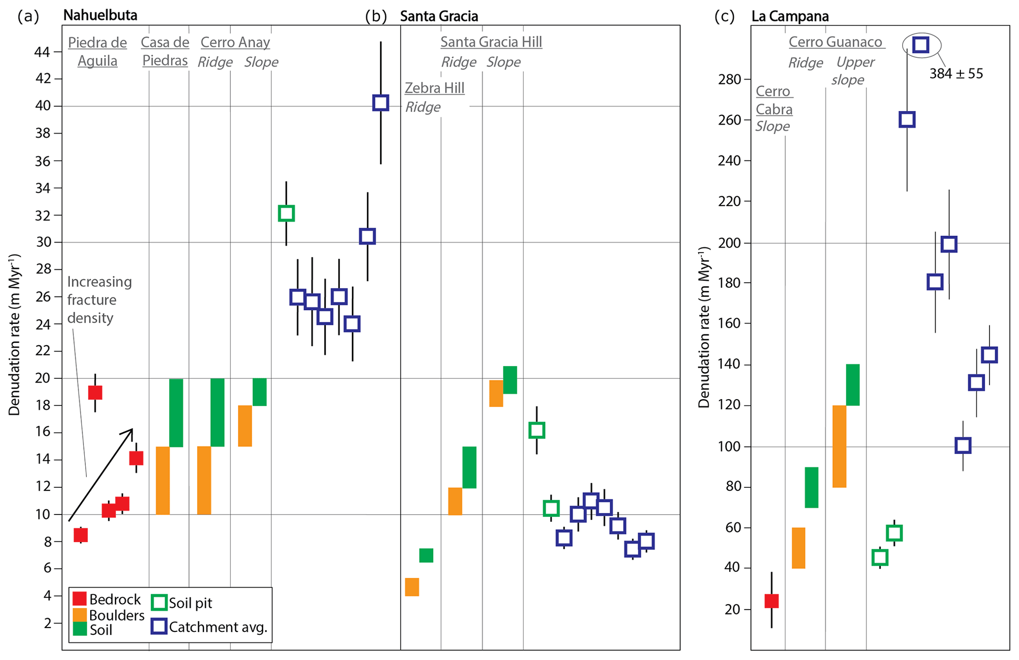
Figure 8Overview of new and previously published denudation rates (data from this study are shown by solid symbols and previously published data are shown by hollow symbols). Soil pit data are from Schaller et al. (2018), and catchment average data are from van Dongen et al. (2019). Catchment average denudation rates from various sediment grain sizes (from left to right for each field site: 0.5–1, 1–2, 2–4, 4–8, 8–16, 16–32, and 32–64 mm). Bedrock denudation rates are calculated using the CRONUS online calculator v2.3 (Balco et al., 2008). Boulder and soil denudation rates are estimated using our model and reflect the most plausible denudation rates as described in Sect. 5.1.2. Denudation rates for each location within a field site are separated by thin gray bars, and locations are labeled at the top of the chart. Samples that were not included in the model (one sample from Nahuelbuta and three samples from La Campana) are also not included here.
5.2 Processes controlling differential erosion
5.2.1 Nahuelbuta (NA)
In NA, the slowest denudation rates occur on bedrock and boulders, likely because precipitation runs off quickly from exposed bedrock, limiting its chemical alteration (Eppes and Keanini, 2017) and weathering (Hayes et al., 2020), whereas soils denude faster. However, denudation rates for soil surrounding the sampled boulders are lower than denudation rates from the soil pit and the catchment average denudation rates. It is possible that boulders physically block soil from being transported downslope: where a dense clustering of exhumed boulders exists, the regolith will be thinner, and the boulders may retard soil erosion throughout the area in which they are clustered (Glade et al., 2017). Considering boulder protrusion and modeled differential erosion rates, boulders in NA are exposed over a long period (up to 640 Kyr), allowing time to affect the long-term transportation of surrounding soil downslope. Although we did not measure sediment damming upslope of boulders in the field, we did note a small amount of sediment damming for boulders on slopes. Away from exhumed boulders, where soil is thicker and where slopes are steep enough, shallow landsliding can occur, as observed in NA by Terweh et al. (2021). In accordance with these observations, van Dongen et al. (2019) found that smaller grains in stream sediment were likely derived from the upper mixed soil layer, and the largest grains were likely excavated from depth, perhaps by shallow landsliding. The smaller grains have denudation rates similar to those presented in this study (Fig. 8), while larger grains have denudation rates similar to deeper soil pit samples from Schaller et al. (2018).
Finally, in NA, where bedrock fracture density is higher, denudation rates are also higher (Fig. 8), likely because precipitation infiltrates into fractures, accelerating chemical weathering, regolith formation (St. Clair et al., 2015; Lebedeva and Brantley, 2017), and subsequent vegetation growth, which introduces biotic acids that further accelerate chemical weathering (Amundson et al., 2007). We further speculate that large exhumed boulders in NA are also sites of less fractured bedrock at depth, as boulders can only be as large as the local fracture spacing allows (e.g., Sklar et al., 2017). Based on the observed differences in soil, boulder, and fractured bedrock denudation rates in NA and on previous studies that have correlated higher fracture density with more rapid erosion (e.g., Dühnforth et al., 2010; DiBiase et al., 2018; Neely et al., 2019), we suggest that bedrock fractures have an effect on NA's morphology through grain size reduction and differential erosion. Further, the thicker soil cover and shallow landsliding on NA slopes may increase the discrepancy between slowly eroding bedrock and boulders versus more rapidly eroding, vegetation-covered hillslopes, eventually causing bedrock and boulders to sit at topographic highs, as we observed in the field.
5.2.2 La Campana (LC)
In LC we observe the largest range of denudation rates between bedrock, boulders, soil, and stream sediment and also the highest overall denudation rates of the three field sites. We suspect that both of these characteristics are related to slope angles, which are on average nearly twice as steep as in NA and SG (Table 1; van Dongen et al., 2019). It should be noted that the stream sediment samples were taken from an adjacent catchment that does not drain the hillslopes sampled in this study, and the generally low and wide-ranging 10Be concentrations in the stream sediment have been related to relatively recent landslides observed in the upper headwaters (van Dongen et al., 2019; Terweh et al., 2021). However, steep slopes are pervasive throughout LC and lead us to suggest that shallow landslides are important erosional processes at this field site.
In LC we frequently observed boulder samples with lower 10Be concentrations than adjacent soil samples (Table 1, Sect. 5.1), which is inconsistent with our simple model of boulder exhumation (Fig. 3) and is possibly because the sampled boulders were not exhumed in situ (Sect. 5.1.1). Landslides as observed in LC can bring down boulders in the process of downhill movement and may cause the excavation of larger blocks from greater depth before their size is reduced in the weathering zone. More vigorous mass wasting is consistent with larger average hillslope grain sizes for LC compared to NA and SG (Terweh et al., 2021). In general, the high relief, steep slopes, and high denudation rates suggest that tectonic uplift rates in LC could be higher than assumed for the nearby coast (Melnick, 2016). Modeled differential denudation rates between boulders and soil are the highest of all field sites, and therefore the time needed to reach the measured boulder protrusion heights is the lowest (23 and 7 Kyr; Table 2), suggesting relatively rapid turnover of boulder exposure and movement downslope. However, we did note some sediment damming by boulders on LC slopes (Fig. 2b3), and in all cases in LC the modeled soil denudation rates are lower than measured soil denudation rates, suggesting that boulders are locally suppressing soil denudation to some extent on LC slopes.
Finally, although the role that fracturing plays in LC is difficult to assess, note that our bedrock sample has a significantly lower denudation rate than boulders and soils (Fig. 8), despite being on a steep slope (Table 1). Rolling and toppling processes that may be relevant for LC boulders are not plausible for the bedrock patch, allowing its nuclide concentration to be high. Likewise, the boulder denudation rate from the ridge sample LC1, where the risk of toppling is likely the lowest, is similar to the bedrock denudation rate. Additionally, LC's Mediterranean climate features frequent fires, which cause spalling of rock flakes off boulder surfaces. While LC boulders are surrounded by shrubs that occasionally burn, causing spalling of boulder surfaces, the extensive bedrock patch in LC is free of vegetation and therefore at a lower risk for fire-induced erosion.
5.2.3 Santa Gracia (SG)
In the semi-arid landscape of SG, as in humid–temperate NA, boulders are eroding more slowly than the surrounding soil, but the differences in boulder and soil denudation rates are subtle. This leads to a slow exposure of hillslope boulders, with exposure of current boulder protrusion (based on differential modeled denudation rates) taking up to 870 Kyr (Table 2). In addition, denudation rate differences between ridge and slope samples – possibly related to slope angle – are larger than the differences between boulders and soil. Furthermore, unlike in NA, our boulder and soil denudation rates are within the same range as the soil pit and catchment average denudation rates (Fig. 8), suggesting that erosional efficiencies are similar across different sediment sizes. Van Dongen et al. (2019) also measured relatively constant catchment average 10Be concentrations over seven grain size classes in SG (Fig. 8), which suggests that all grain sizes have been transported from the upper mixed layer of hillslope soil and that deep-seated erosion processes are unlikely, in accordance with absent landsliding (Terweh et al., 2021). Thus, our results agree with previous findings that erosion in SG is likely limited to grain-by-grain exfoliation of boulders and the slow diffusive creep of the relatively thin soil cover on hillslopes (Schaller et al., 2018). When bedrock is exhumed, its long residence time on hillslopes allows it to weather slowly in place and be reduced in size, with minimal transportation of weathered material by runoff and a low degree of chemical weathering and soil production (Schaller and Ehlers, 2022).
Such a narrow range of relatively low denudation rates indicates that very long time periods are necessary to produce relief between hilltops and valleys. Note, however, that despite low uplift rates in SG, the total mean basin slope in SG is 17∘ compared to 9∘ in NA (van Dongen et al., 2019). This could be due to low mean annual precipitation, resulting in a low erosional efficiency in SG, which, in order to achieve denudation rates that match uplift rates, requires the slopes to be steeper (Carretier et al., 2018). Although the differences in denudation rates between grain sizes are subtle in SG, soils have higher denudation rates than the boulders they directly surround. Additionally, the measured denudation rates of soil surrounding boulders on SG slopes are lower than modeled soil denudation rates (Table 2), indicating that boulders may be prolonging the residence time of the surrounding soil by a small amount, either by blocking its movement downslope or by contributing grains through exfoliation.
5.3 Fracture control on larger-scale landscape evolution
We have shown that, at our field sites, bedrock denudes the slowest, followed by boulders and finally soil. In each climate zone, especially where chemical weathering plays a large role (NA), sediment size is likely controlled by the spacing of bedrock fractures. Once on the surface, on low or moderate slopes, large boulders initially delineated by fracture spacing are more difficult to transport than smaller sediment and therefore locally retard denudation rates. On the landscape scale, such differential erosion should lead to landscape morphologies controlled by fracture spacing patterns. In NA, we were able to measure fracture density in several bedrock outcrops and found that average higher fracture density is correlated with higher denudation rates (Fig. 5a). It is plausible that the measured fracture spacing in bedrock outcrops represents the parts of the landscape where bedrock fracture density is the lowest, and it is highest under the soil-mantled parts of the landscapes, where fractures are not exposed. Fracture spacing in NA is generally larger than boulder width (Fig. 5c), although there is overlap. If we assume that boulder width is initially delineated by fracture spacing at depth, our results indicate that boulders have been reduced in size in the weathering zone prior to and during exhumation. If we further assume that hillslope sediment lies on a spectrum with unweathered blocks delineated by fractures on one end and sediment that has been significantly reduced in size in the weathering zone on the other end (e.g., Verdian et al., 2021), boulders in NA seem to fall somewhere in the middle.

Figure 9Schematic illustration showing the influence of bedrock fractures on landscape evolution. (a) Bedrock with different fracture densities is infiltrated to different degrees by rain and groundwater, which leads to differences in chemical weathering, soil formation, and vegetation growth, resulting in different hillslope sediment sizes. (b) Differential denudation between highly fractured and less fractured areas induces relief growth under slow but persistent uplift, which further promotes spatial gradients in chemical weathering, hillslope sediment size, and denudation. (c) Growing relief increases topographic stresses and the formation of new fractures (red) at topographically high positions (e.g., St. Clair et al., 2015) as well as unloading-related surface-parallel fractures (dark blue) (e.g., Martel, 2011), and steeper slopes allow for transportation of boulders, shown rolling down the slopes on either side.
Bedrock fracture patterns also likely affect stream incision in a similar way by dissecting bedrock and reducing sediment size, making it easier to transport by flowing water. This phenomenon may be visible at our field sites on a larger scale through the similarity of fault and stream orientations. In NA, our fracture orientation measurements (Fig. 5b) are similar to fault and stream orientations (Fig. 7). In general, as tectonically induced faults and fractures are products of the same regional stresses, we assume that regional faults have orientations consistent with fractures at our field sites (see Krone et al., 2021). Regional faults and smaller fractures have been shown to be closely related: Rodriguez Padilla et al. (2022) mapped fractures resulting from the 2019 Ridgecrest earthquakes in bedrock and sediment-covered areas and found that fracture density decreases from main faults with a power-law distribution. They also found that the orientations of faults and fractures closely matched. Fracture orientation has also been shown to influence stream orientation. Roy et al. (2015) modeled stream incision in a landscape dissected by dipping weak zones, meant to resemble fracture or fault zones, and found that in cases with a large contrast in bedrock weakness (), channels migrated laterally to follow the shifting exhumation of the weak zone. At our field sites, we observe that stream channels (Amin≥105 m2) generally follow fault orientations (Fig. 7). This is especially clear in SG, where the north–south-striking Atacama Fault System is reflected in the orientation of faults, streams, and also fractures measured in a nearby drill core (Krone et al., 2021; Fig. 7). In LC and NA, despite more variety in fault and stream orientations, streams closest to the field sites tend to align with fault orientations (Fig. 7). Especially in NA, the larger streams are often nearly perpendicular to each other, similar to rectangular drainage networks, which are often indicative of structural control on drainage patterns (e.g., Zernitz, 1932). These results suggest that within the same rock type, local fracture patterns induced by regional faults can induce differential denudation in landscapes.
In summary, we argue that in NA, and possibly also in SG and LC, bedrock fracturing influences landscape morphology by setting grain size and thus dictating patterns of denudation rates on hillslopes and in streams: in situ hillslope boulders likely originated as blocks set by fracture spacing and, after being exhumed, locally suppress denudation as described above. This interpretation is supported by work in Puerto Rico; Buss et al. (2013) studied corestones from two boreholes cutting through regolith in the Luquillo Experimental Forest and found that corestones decreased in size with increased chemical weathering and exhumation through the regolith profile. They deduced that the corestones likely started as bedrock blocks delineated by fractures. Further, they found that the borehole drilled near a stream channel contained more highly fractured bedrock compared to the borehole drilled at a ridge and inferred that corestone size was larger under the ridge due to lower bedrock fracture density. In accordance with Fletcher and Brantley (2010), they concluded that, if erosion and weathering increase with bedrock fracture density, then the ridges and valleys in their study area could be controlled by fracture density patterns.
We therefore offer the following conceptual model: in a landscape with fractured bedrock (Fig. 9a), areas with higher fracture density should be sites of smaller hillslope sediment sizes (e.g., Sklar et al., 2017; Neely and DiBiase, 2020), where rainfall can easily infiltrate, conversion of bedrock to regolith is easiest (St. Clair et al., 2015; Lebedeva and Brantley, 2017), and denudation rates are highest. Over time, precipitation will divergently run off topographic highs and starve bedrock and larger boulders on high points while infiltrating into topographic lows, where streams eventually incise (Bierman, 1994; Hayes et al., 2020; Fig. 9b). Bedrock and boulders on topographic highs denude more slowly than finer sediment and soil, accentuating any elevation differences. Regolith also promotes vegetation growth, which slows runoff, raises rates of infiltration, and enhances chemical weathering (Amundson et al., 2007; Fig. 9b). In steeper landscapes, such as LC, boulders will be more mobile and may roll down the hillslopes, eventually ending up in stream channels where they may shield the channel bed from denudation (DiBiase et al., 2017; Shobe et al., 2016; Fig. 9c). In addition, in such higher-relief landscapes, fractures due to topographic stresses from exhumation may form at topographic highs as the topography emerges (St. Clair et al., 2015), countering this positive feedback loop (Fig. 9c). Over longer timescales, bedrock with different patterns of fracture density may be exhumed, which can invert landscapes to reflect the new fracture patterns exposed at the surface (Roy et al., 2016). In this way, fracturing, climate, and residence time can operate in conjunction to set the sediment size and morphology of hillslopes and streams within landscapes.
In this study, we explored the ability of bedrock patches and large boulders to retard denudation and influence landscape morphology in three relatively slowly eroding landscapes along a climate gradient in the Chilean Coastal Cordillera. Based on in situ cosmogenic 10Be-derived denudation rates of bedrock, boulders, and soil, we find that in almost all cases across the three sites studied, soil denudation rates are ∼10 %–50 % higher than the denudation rates of the boulders that they surround, which are more similar to bedrock denudation rates. This pattern is more complicated in La Campana, where some boulders have lower 10Be concentrations than the surrounding soil, perhaps because they were overturned or covered with soil at some point due to steeper slopes. These results suggest that exposed bedrock patches and large hillslope boulders affect landscape morphology by slowing denudation rates, eventually forming the nucleus for topographic highs. On the other hand, our work also suggests that where slopes are close to the angle of repose and where landsliding is observed (as in La Campana), while bedrock patches denude slowly and likely retard hillslope denudation, hillslope boulders may have a smaller or even negligible effect on suppressing denudation.
In addition, we found that bedrock fracturing and faulting accelerate hillslope denudation and stream incision at our field sites: hillslope denudation rates increase with fracture density in NA, and streams tend to follow the orientation of larger faults at all three sites. We infer that bedrock fracture patterns at our field sites set grain sizes on hillslopes, and bedrock patches and boulders represent locations where fracture density is lower; thus, weathering, erosion, and soil formation are suppressed. On a larger scale, our results imply that tectonic preconditioning in the form of bedrock faulting and fracturing influences landscape evolution by impacting the pathway of streams, as well as the migration of ridges, as landscapes denude through layers of bedrock preconditioned by tectonic fracturing over time and encounter varying levels of resistance depending on the fracture density.
Cosmogenic nuclide data and MATLAB scripts of the model presented in this paper will be made available as a GFZ Data Publication in accordance with FAIR principles. Lidar data from the studied catchments are available in Krüger et al. (2022) (https://doi.org/10.5880/fidgeo.2022.002).
The supplement related to this article is available online at: https://doi.org/10.5194/esurf-11-305-2023-supplement.
DS conceived the initial idea for this project. EL, DS, and RvD performed fieldwork. EL performed the laboratory work, with support from HW. EL, DS, and HW analyzed the data. EL wrote the paper with support from DS, HW, and RvD.
The contact author has declared that none of the authors has any competing interests.
Publisher's note: Copernicus Publications remains neutral with regard to jurisdictional claims in published maps and institutional affiliations.
This article is part of the special issue “Earth surface shaping by biota (Esurf/BG/SOIL/ESD/ESSD inter-journal SI)”. It is not associated with a conference.
We are very grateful to the EarthShape management, Friedhelm von Blanckenburg and Todd Ehlers, and the EarthShape coordinators Kirstin Übernickel and Leandro Paulino. We also thank the Chilean National Park Service (CONAF) for providing access to the sample locations and on-site support of our research. We also thank Iris Eder and David Scheer for their help in the field and in the laboratory, Cathrin Schulz for her help in the laboratory, and Steven A. Binnie and Stefan Heinze from Cologne University for conducting AMS measurements. Finally, we thank the two anonymous reviewers, whose comments helped to improve the paper.
This research has been supported by the Deutsche Forschungsgemeinschaft (EarthShape: Earth Surface Shaping by Biota grant SCHE 1676/4-2 to Dirk Scherler).
The article processing charges for this open-access publication were covered by the Helmholtz Centre Potsdam – GFZ German Research Centre for Geosciences.
This paper was edited by Fiona Clubb and reviewed by two anonymous referees.
Alaska Satellite Facility Distributed Active Archive Center: ALOS PALSAR_Radiometric_Terrain_Corrected_high_res (ALPSRP191976520), DEM for La Campana, includes Material © JAXA/METI 2009, ASF DAAC [data set], https://doi.org/10.5067/Z97HFCNKR6VA, 2009.
Alaska Satellite Facility Distributed Active Archive Center: ALOS PALSAR_Radiometric_Terrain_Corrected_high_res (ALPSRP269644390), DEM for Nahuelbuta, includes Material © JAXA/METI 2011, ASF DAAC [data set], https://doi.org/10.5067/Z97HFCNKR6VA, 2011a.
Alaska Satellite Facility Distributed Active Archive Center: ALOS PALSAR_Radiometric_Terrain_Corrected_high_res (ALPSRP277746590), DEM for Santa Gracia, includes Material © JAXA/METI 2011, ASF DAAC [data set], https://doi.org/10.5067/Z97HFCNKR6VA, 2011b.
Amundson, R., Richter, D. D., Humphreys, G. S., Jobbágy, E. G., and Gaillardet, J.: Coupling between biota and earth materials in the critical zone, Elements, 3, 327–333, https://doi.org/10.2113/gselements.3.5.327, 2007.
Attal, M., Mudd, S. M., Hurst, M. D., Weinman, B., Yoo, K., and Naylor, M.: Impact of change in erosion rate and landscape steepness on hillslope and fluvial sediments grain size in the Feather River basin (Sierra Nevada, California), Earth Surf. Dynam., 3, 201–222, https://doi.org/10.5194/esurf-3-201-2015, 2015.
Balco, G., Stone, J. O., Lifton, N. A., and Dunai, T. J.: A complete and easily accessible means of calculating surface exposure ages or erosion rates from 10Be and 26Al measurements, Quatern. Geochronol., 3, 174–195, https://doi.org/10.1016/j.quageo.2007.12.001, 2008.
Bierman, P.: Using in situ produced cosmogenic isotopes to estimate rates of Landscape evolution: A review from the geomorphic perspective, J. Geophys. Res.-Solid, 99, 13885–13896, https://doi.org/10.1029/94JB00459, 1994.
Bierman, P. R. and Caffee, M. W.: Cosmogenic exposure and erosion history of Australian rock landforms, Geol. Soc. Am. Bull., 114, 787–803, https://doi.org/10.1130/0016-7606(2002)114<0787:CEAEHO>2.0.CO;2, 2002.
Boisier, J. P., Alvarez-Garretón, C., Cepeda, J., Osses, A., Vásquez, N., and Rondanelli, R.: CR2MET: A high-resolution precipitation and temperature dataset for hydroclimatic research in Chile, in: EGU General Assembly 2018, April 2018, Vienna, Austria, EGU2018-19739, 2018.
Borchers, B., Marrero, S., Balco, G., Caffee, M., Goehring, B., Lifton, N., Nishiizumi, K., Phillips, F., Schaefer, J., and Stone, J.: Geological calibration of spallation production rates in the CRONUS-Earth project, Quatern. Geochronol., 31, 188-198, https://doi.org/10.1016/j.quageo.2015.01.009, 2016.
Braucher, R., Merchel, S., Borgomano, J., and Bourlès, D.L.: Production of cosmogenic radionuclides at great depth: A multi element approach, Earth Planet. Sc. Lett., 309, 1–9, https://doi.org/10.1016/j.epsl.2011.06.036, 2011.
Burbank, D. W., Leland, J., Fielding, E., Anderson, R. S., Brozovic, N., Reid, M. R., and Duncan, C.: Bedrock incision, rock uplift and threshold hillslopes in the northwestern Himalayas, Nature, 379, 505–510, https://doi.org/10.1038/379505a0, 1996.
Buss, H. L., Brantley, S. L., Scatena, F. N., Bazilievskaya, E. A., Blum, A., Schulz, M., Jiménez, R., White, A. F., Rother, G., and Cole, D.: Probing the deep critical zone beneath the Luquillo Experimental Forest, Puerto Rico, Earth Surf. Proc. Land., 38, 1170-1186, https://doi.org/10.1002/esp.3409, 2013.
Carretier, S., Tolorza, V., Regard, V., Aguilar, G., Bermúdez, M. A., Martinod, J., Guyot, J.-L., Hérail, G., and Riquelme, R.: Review of erosion dynamics along the major N–S climatic gradient in Chile and perspectives, Geomorphology, 300, 45–68, https://doi.org/10.1016/j.geomorph.2017.10.016, 2018.
Chilton, K. D. and Spotila, J. A.: Preservation of Valley and Ridge topography via delivery of resistant, ridge-sourced boulders to hillslopes and channels, Southern Appalachian Mountains, USA, Geomorphology, 365, 107263, https://doi.org/10.1016/j.geomorph.2020.107263, 2020.
Coira, B., Davidson, J., Mpodozis, C., and Ramos, V.: Tectonic and Magmatic Evolution of the Andes of Northern Argentina and Chile, Earth Sci Rev., 18, 303–332, https://doi.org/10.1016/0012-8252(82)90042-3, 1982.
Dewald, A., Heinze, S., Jolie, J., Zilges, A., Dunai, T., Rethemeyer, J., Melles, M., Staubwasser, M., Kuczewski, B., Richter, J., Radtke, U., von Blanckenburg, F., and Klein, M.: Cologne AMS, a dedicated center for accelerator mass spectrometry in Germany, Nucl. Instrum. Meth. B, 294, 18–23, https://doi.org/10.1016/j.nimb.2012.04.030, 2013.
DiBiase, R. A., Lamb, M. P., Ganti, V., and Booth, A. M.: Slope, grain size, and roughness controls on dry sediment transport and storage on steep hillslopes, J. Geophys. Res.-Earth Surf., 122, 941–960, https://doi.org/10.1002/2016JF003970, 2017.
DiBiase, R. A., Rossi, M. W., and Neely, A. B.: Fracture density and grain size controls on the relief structure of bedrock landscapes, Geology, 46, 399–402, https://doi.org/10.1130/G40006.1, 2018.
Dietrich, W. E., Bellugi, D. G., Sklar, L. S., Stock, J. D., Heimsath, A. M., and Roering, J. J.: Geomorphic transport laws for predicting landscape form and dynamics, Geophys. Monogr., 135, 103–132, https://doi.org/10.1029/135GM09, 2003.
Dühnforth, M., Anderson, R. S., Ward, D., and Stock, G. M.: Bedrock fracture control of glacial erosion processes and rates, Geology, 38, 423–426, https://doi.org/10.1130/G30576.1, 2010.
Eppes, M. C. and Keanini, R..: Mechanical weathering and rock erosion by climate-dependent subcritical cracking, Rev. Geophys., 55, 470–508, https://doi.org/10.1002/2017RG000557, 2017.
Fletcher, R. C. and Brantley, S. L.: Reduction of bedrock blocks as corestones in the weathering profile: Observations and model, Am. J. Sci., 310, 131–164, https://doi.org/10.2475/03.2010.01, 2010.
Glade, R. C., Anderson, R. S., and Tucker, G. E.: Block-controlled hillslope form and persistence of topography in rocky landscape, Geology, 45, 311–314, https://doi.org/10.1130/G38665.1, 2017.
Glodny, J., Graaefe, K., and Rosenau, M.: Mesozoic to Quaternary continental margin dynamics in South-Central Chile (36–42∘ S): the apatite and zircon fission track perspective, Int. J. Earth Sci., 97, 1271–1291, https://doi.org/10.1007/s00531-007-0203-1, 2008.
Granger, D. E., Riebe, C. S., Kirchner, J. W., and Finkel, R. C.: Modulation of erosion on steep granitic slopes by boulder armoring, as revealed by cosmogenic 26Al and 10Be, Earth Planet. Sc. Lett., 186, 269–281, https://doi.org/10.1016/S0012-821X(01)00236-9, 2001.
Granger, D. E. and Riebe, C. S.: Cosmogenic Nuclides in Weathering and Erosion, in: Treatise on Geochemistry, 2nd Edn., edited by: Holland, H. D. and Turekian, K. K., Elsevier, Oxford, 7, 401–436, https://doi.org/10.1016/B978-0-08-095975-7.00514-3, 2014.
Hayes, N. R., Buss, H. L., Moore, O. W., Krám, P., and Pancost, R. D.: Controls on granitic weathering fronts in contrasting climates, Chem. Geol., 535, 119450, https://doi.org/10.1016/j.chemgeo.2019.119450, 2020.
Heimsath, A. M., Chappell, J., Dietrich, W. E., Nishiizumi, K., and Finkel, R. C.: Soil production on a retreating escarpment in southeastern Australia, Geology, 28, 787–790, https://doi.org/10.1130/0091-7613(2000)28<787:SPOARE>2.0.CO;2, 2000.
Heimsath, A. M., Chappell, J., Dietrich, W. E., Nishiizumid, K., and Finkel, R. C.: Late Quaternary erosion in southeastern Australia: a field example using cosmogenic nuclides, Quatern. Int., 83, 169–185, https://doi.org/10.1016/S1040-6182(01)00038-6, 2001.
Kirby, E. and Whipple, K. X.: Expression of active tectonics in erosional landscapes, J. Struct. Geol., 44, 54–75, https://doi.org/10.1016/j.jsg.2012.07.009, 2012.
Krone, L.V., Hampl, F. J., Schwerdhelm, C., Bryce, C., Ganzert, L., Kitte, A., Übernickel, K., Dielforder, A., Aldaz, S., Oses-Pedraza, R., and Perez, J. P. H.: Deep weathering in the semi-arid Coastal Cordillera, Chile, Sci. Rep., 11, 1–15, 2021.
Kügler, M., Hoffmann, T. O., Beer, A. R., Übernickel, K., Ehlers, T. A., Scherler, D., and Eichel, J.: (LiDAR) 3D Point Clouds and Topographic Data from the Chilean Coastal Cordillera, V. 1.0, GFZ Data Services [data set], https://doi.org/10.5880/fidgeo.2022.002, 2022.
Lal, D.: Cosmic ray labeling of erosion surfaces: in situ nuclide production rates and erosion models, Earth Planet. Sc. Lett., 104, 424–439, https://doi.org/10.1016/0012-821X(91)90220-C, 1991.
Lamb, M. P., Finnegan, N. J., Scheingross, J. S. and Sklar, L. S.: New insights into the mechanics of fluvial bedrock erosion through flume experiments and theory, Geomorphology, 244, 33–55, https://doi.org/10.1016/j.geomorph.2015.03.003, 2015.
Lebedeva, M. I. and Brantley, S. L.: Weathering and erosion of fractured bedrock systems, Earth Surf. Proc. Land., 42, 2090–2108, https://doi.org/10.1002/esp.4177, 2017.
Martel, S. J.: Mechanics of curved surfaces, with application to surface-parallel cracks, Geophys. Res. Lett., 38, L20303, https://doi.org/10.1029/2011GL049354, 2011.
Melnick, D.: Rise of the central Andean coast by earthquakes straddling the Moho, Nat. Geosci., 9, 1–8, https://doi.org/10.1038/ngeo2683, 2016.
Molnar, P., Anderson, R. S., and Anderson, S. P.: Tectonics, fracturing of rock, and erosion, J. Geophys. Res., 112, F03014, https://doi.org/10.1029/2005JF000433, 2007.
Neely, A. B. and DiBiase, R. A.: Drainage Area, Bedrock Fracture Spacing, and Weathering Controls on Landscape-Scale Patterns in Surface Sediment Grain Size, J. Geophys. Res.-Earth, 125, e2020JF005560, https://doi.org/10.1029/2020JF005560, 2020.
Neely, A. B., DiBiase, R. A., Corbett, L. B., Bierman, P. R., and Caffee, M. W.: Bedrock fracture density controls on hillslope erodibility in steep, rocky landscapes with patchy soil cover, southern California, USA, Earth Planet. Sc. Lett., 522, 186–197, https://doi.org/10.1016/j.epsl.2019.06.011, 2019.
Oeser, R. A., Stroncik, N., Moskwa, L., Bernhard, N., Schaller, M., Canessa, R., Van Den Brink, L., Köster, M., Brucker, E., Stock, S., Pablo, J., Godoy, R., Javier, F., Oses, R., Osses, P., Paulino, L., Seguel, O., Bader, M. Y., Boy, J., Dippold, M. A., Ehlers, T. A., Kühn, P., Kuzyakov, Y., Leinweber, P., Scholten, T., Spielvogel, S., Spohn, M., Übernickel, K., Tielbörger, K., Wagner, D., and von Blanckenburg, F.: Chemistry and microbiology of the Critical Zone along a steep climate and vegetation gradient in the Chilean Coastal Cordillera, Catena, 170, 183–203, https://doi.org/10.1016/j.catena.2018.06.002, 2018.
Perron, J. T.: Numerical methods for nonlinear hillslope transport laws, J. Geophys. Res.-Earth, 116, 2021, https://doi.org/10.1029/2010JF001801, 2011.
Portenga, E. W. and Bierman, P. R.: Understanding earth's eroding surface with 10Be, GSA Today, 21, 4–10, https://doi.org/10.1130/G111A.1, 2011.
Raab, G., Egli, M., Norton, K., Dahms, D., Brandová, D., Christl, M., and Scarciglia, F.: Climate and relief-induced controls on the temporal variability of denudation rates in a granitic upland, Earth Surf. Proc. Land., 44, 2570–2586, https://doi.org/10.1002/esp.4681, 2019.
Riebe, C. S. and Granger, D. E.: Quantifying effects of deep and near-surface chemical erosion on cosmogenic nuclides in soils, saprolite, and sediment, Earth Surf. Proc. Land., 38, 523–533, https://doi.org/10.1002/esp.3339, 2013.
Roda-Boluda, D. C., D'Arcy, M., McDonald, J., and Whittaker, A. C.: Lithological controls on hillslope sediment supply: insights from landslide activity and grain size distributions, Earth Surf. Proc. Land., 43, 956–977, https://doi.org/10.1002/esp.4281, 2018.
Rodriguez Padilla, A. M., Oskin, M. E., Milliner, C. W., and Plesch, A.: Accrual of widespread rock damage from the 2019 Ridgecrest earthquakes, Nat. Geosci., 15, 222–226, 2022.
Roy, S. G., Koons, P. O., Upton, P., and Tucker, G. E.: The influence of crustal strength fields on the patterns and rates of fluvial incision, J. Geophys. Res.-Earth, 120, 275–299, https://doi.org/10.1002/2014JF003281, 2015.
Roy, S. G., Tucker, G. E., Koons, P. O., Smith, S. M., and Upton, P.: A fault runs through it: Modeling the influence of rock strength and grain-size distribution in a fault-damaged landscape, J. Geophys. Res.-Earth, 121, 1911–1930, https://doi.org/10.1002/2015JF003662, 2016.
Schaller, M. and Ehlers, T. A.: Comparison of soil production, chemical weathering, and physical erosion rates along a climate and ecological gradient (Chile) to global observations, Earth Surf. Dynam., 10, 131–150, https://doi.org/10.5194/esurf-10-131-2022, 2022.
Schaller, M., Ehlers, T. A., Lang, K. A. H., Schmid, M., and Fuentes-Espoz, J. P.: Addressing the contribution of climate and vegetation cover on hillslope denudation, Chilean Coastal Cordillera (26∘–38∘ S), Earth Planet. Sc. Lett., 489, 111–122, https://doi.org/10.1016/j.epsl.2018.02.026, 2018.
Schwanghart, W. and Scherler, D.: Short Communication: Topo Toolbox 2 – MATLAB-based software for topographic analysis and modeling in Earth surface sciences, Earth Surf. Dynam., 2, 1–7, https://doi.org/10.5194/esurf-2-1-2014, 2014.
SERNAGEOMIN: Mapa Geológico de Chile: versión digital, Servicio Nacional de Geología y Minería, Publicación Geológica Digital No. 4, SERNAGEOMIN [data set], http://www.ipgp.fr/~dechabal/Geol-millon.pdf (last access: 5 April 2022), 2003.
Shobe, C. M., Tucker, G. E., and Anderson, R. S.: Hillslope-derived blocks retard river incision, Geophys. Res. Lett., 43, 5070–5078, https://doi.org/10.1002/2016GL069262, 2016.
Sklar, L. S. and Dietrich, W. E.: Sediment and rock strength controls on river incision into bedrock, Geology, 29, 1087–1090, https://doi.org/10.1130/0091-7613(2001)029<1087:SARSCO>2.0.CO;2, 2001.
Sklar, L. S., Riebe, C. S., Marshall, J. A., Genetti, J., Leclere, S., Lukens, C. L., and Merces, V.: The problem of predicting the size distribution of sediment supplied by hillslopes to rivers, Geomorphology, 277, 31–49, https://doi.org/10.1016/j.geomorph.2016.05.005, 2017.
Sklar, L. S., Riebe, C. S., Genetti, J., Leclere, S., and Lukens, C. E.: Downvalley fining of hillslope sediment in an alpine catchment: implications for downstream fining of sediment flux in mountain rivers, Earth Surf. Proc. Land., 45, 1828–1845, https://doi.org/10.1002/esp.4849, 2020.
Small, E. E., Anderson, R. S., Repka, J. L., and Finkel, R.: Erosion rates of alpine bedrock summit surfaces deduced from in situ 10Be and 26A1, Earth Planet. Sc. Lett., 150, 413–425, https://doi.org/10.1016/S0012-821X(97)00092-7, 1997.
St. Clair, J., Moon, S., Holbrook, W. S., Perron, J. T., Riebe, C. S., and Martel, S. J.: Geophysical imaging reveals topographic stress control of bedrock weathering, Geomorphology, 350, 534–538, https://doi.org/10.1126/science.aab2210, 2015.
Stone, J. O.: Air pressure and cosmogenic isotope production, J. Geophys. Res.-Solid, 105, 23753–23759, https://doi.org/10.1029/2000JB900181, 2000.
Terweh, S., Hassan, M. A., Mao, L., Schrott, L., and Hoffmann, T. O.: Bio-climate affects hillslope and fluvial sediment grain size along the Chilean Coastal Cordillera, Geomorphology, 384, 107700, https://doi.org/10.1016/j.geomorph.2021.107700, 2021.
Thaler, E. A. and Covington, M. D.: The influence of sandstone caprock material on bedrock channel steepness within a tectonically passive setting: Buffalo National River Basin, Arkansas, USA, J. Geophys. Res.-Earth, 121, 1635–1650, https://doi.org/10.1002/2015JF003771, 2016.
van Dongen, R., Scherler, D., Wittmann, H., and von Blanckenburg, F.: Cosmogenic 10Be in river sediment: where grain size matters and why, Earth Surf. Dynam., 7, 393–410, https://doi.org/10.5194/esurf-7-393-2019, 2019.
Verdian, J. P., Sklar, L. S., Riebe, C. S., and Moore, J. R.: Sediment size on talus slopes correlates with fracture spacing on bedrock cliffs: implications for predicting initial sediment size distributions on hillslopes, Earth Surf. Dynam., 9, 1073–1090, https://doi.org/10.5194/esurf-9-1073-2021, 2021.
von Blanckenburg, F., Hewawasam, T., and Kubik, P. W.: Cosmogenic nuclide evidence for low weathering and denudation in the wet, tropical highlands of Sri Lanka, J. Geophys. Res., 109, F03008, https://doi.org/10.1029/2003JF000049, 2004.
Zernitz, E. R.: Drainage patterns and their significance, J. Geol., 40, 498–521, https://doi.org/10.1086/623976, 1932.
The requested paper has a corresponding corrigendum published. Please read the corrigendum first before downloading the article.
- Article
(4902 KB) - Full-text XML
- Corrigendum
-
Supplement
(702 KB) - BibTeX
- EndNote