Spatially coherent variability in modern orographic precipitation produces asymmetric paleo-glacier extents in flowline models: Olympic Mountains, USA

Glaciers are sensitive to temporal climate variability. Glacier sensitivity to spatial variability in climate has been much less studied. The Olympic Mountains of Washington state, USA, experience a pronounced orographic precipitation gradient, with modern annual precipitation ranging between ∼6500 and ∼500 mm water equivalent. In the Quinault valley, on the wet side of the range, a glacier extended onto the coastal plain, reaching a maximum position during the Early Wisconsin glaciation. On the dry side of the range, in the Elwha valley, there is no evidence of a large paleo-glacier during the Wisconsin glaciation. We hypothesize that asymmetry in the past glacier extent was driven by spatial variability in precipitation. To evaluate this hypothesis, we constrain the past precipitation gradient and model the glacier extent. We explore variability in observed and modeled precipitation gradients over timescales from 6 h to ∼100 yr. Across three datasets, basin-averaged precipitation in the Elwha is 54 % of that in the Quinault. Our analysis overwhelmingly indicates spatially coherent variability in precipitation across the peninsula. We conclude that the past precipitation gradient was likely similar to the modern gradient. We use a one-dimensional glacier flowline model, driven by sea level summer temperature and annual precipitation to approximate the glacier extent in the Quinault and Elwha valleys. We find several equilibrium states for the Quinault glacier at the mapped maximum position within paleoclimate constraints for cooling and drying, relative to present-day conditions. Assuming stable precipitation gradients, we model the Elwha glacier extent for the climates of these equilibria. At the warm end of the paleoclimate constraint (July average sea level temperature of 10.5 ^∘C), a small valley glacier occurs in the high headwaters of the Elwha valley. Yet, for the cooler end of the allowable paleoclimate (July average sea level temperature of 7 ^∘C), the Elwha glacier advances to a narrow notch in the valley, thickens, and rapidly extends far beyond the likely true maximum extent. Therefore, we suggest that the Early Wisconsin period was more likely to have been relatively warm because our models of the glacial extent are consistent with the past record of glaciation in both the Quinault valley and Elwha valley for warm conditions but inconsistent for cooler conditions. Alternatively, spatially variable drivers of ablation, including differences in cloudiness, could have contributed to past asymmetry in the glacier extent. Future research to constrain past precipitation gradients and evaluate their impact on glacier dynamics is needed to better interpret the climatic significance of past glaciation and to predict the future response of glaciers to climate change.

1 Introduction

Glaciers are sensitive indicators of climate change through time because glacier extent is dependent on climate variables including precipitation, temperature, insolation, and cloudiness (e.g., Braithwaite et al., 2003; Wagnon et al., 2003; Kessler et al., 2006; Rupper and Roe, 2008; Anders et al., 2010). The sensitivity of glaciers to climate has been used to interpret past changes and predict future changes in glacier extent as a response to, and record of, temporal changes in climate (Oerlemans et al., 1998; Roe, 2011). However, climate not only varies in time but also in space. Spatial variability in precipitation due to topographic forcing (i.e., a rain shadow) is a well-documented and generally well-understood example of a robust spatial gradient in climate (Roe, 2005). How does glacier extent vary across a mountain range with a significant rain shadow? We consider this question for the Olympic Mountains of Washington state, USA (Fig. 1a and b). This mountain range on the Pacific Northwest coast has small modern glaciers and evidence of extensive glaciation during the Pleistocene (Thackray, 2001). We begin by assessing the possibility of significant changes in the rain shadow strength during glacial conditions relative to the present. Having established that spatial gradients in precipitation are likely a robust feature of the climate of the Olympic Mountains, we simulate the evolution of glaciers on the windward and leeward side of the range to examine the impact of the rain shadow on the size of glaciers.

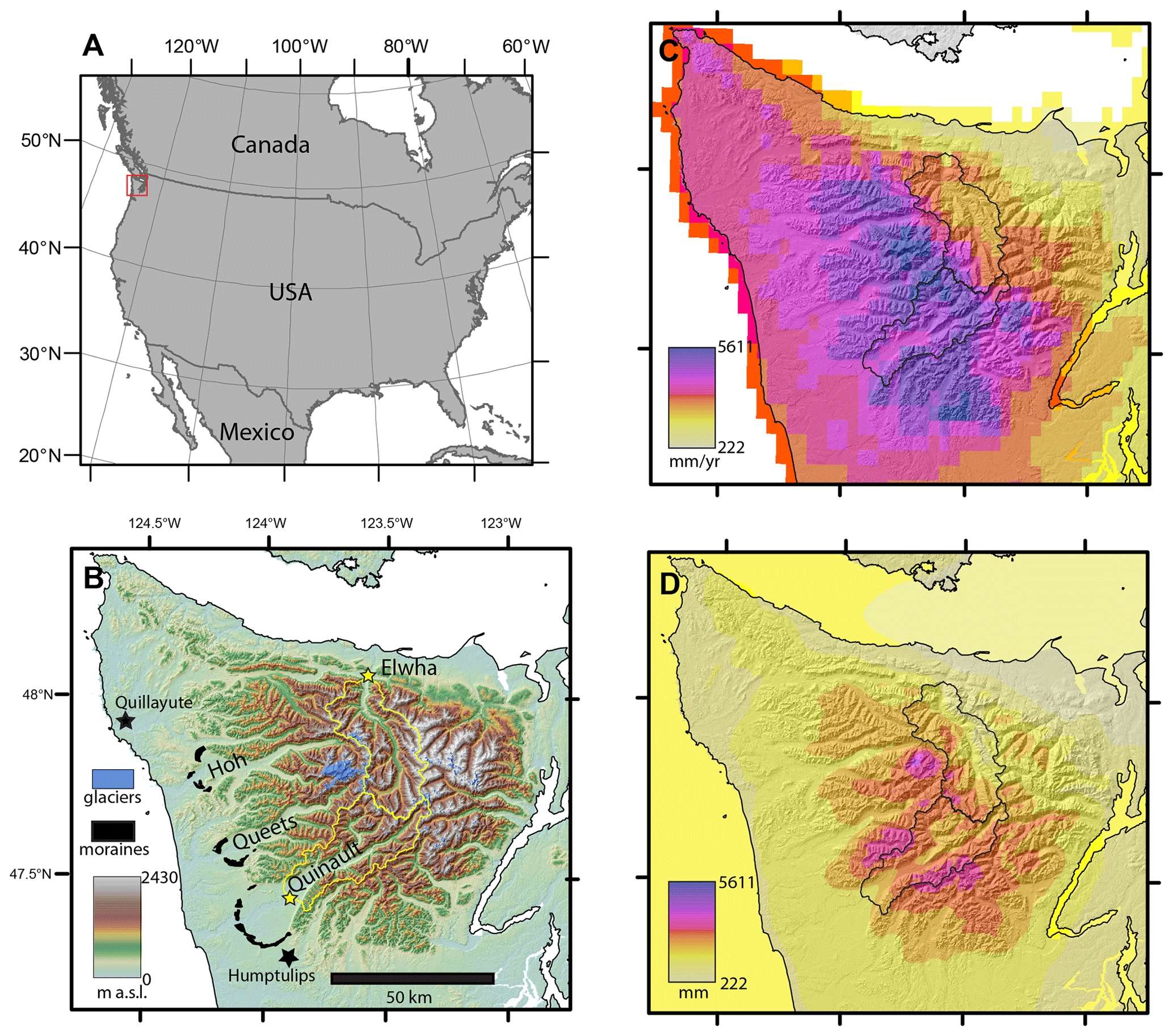
Figure 1 Panel (a) shows location of the study area in Washington state, USA. Panel (b) shows the topography of the Olympic Peninsula. Terminal moraines of the west side valleys are shown in black (Marshall, 2013; Staley, 2015). Radiosondes are routinely launched from the black star at Quillayute (Rutledge and Ciesielski, 2016). Humptulips (black star) is the location of the paleoclimate record we use. We define the Elwha and Quinault basins (outlined in yellow) as the regions upstream of USGS stream gauges, which are shown as yellow stars. Panel (c) shows the annual climatological precipitation from the PRISM model (Daly et al., 2008). Panel (d) shows the total modeled precipitation during the OLYMPEX campaign in the winter of 2015–2016 (Skamarock et al., 2008).

Modern precipitation across the Olympic Mountains is characterized by a steep precipitation gradient (e.g., Hobbs, 1978; Anders et al., 2007; Cao et al., 2018). Annual precipitation varies from ∼6500 mm w.e. (water equivalent) at high elevations on the western side of the range to ∼500 mm w.e. on the northeastern lowlands (Fig. 1c). On the Pacific coast, monthly precipitation totals during the drier warm season (May–September) vary from ∼50 to 150 mm per month. In contrast, the average monthly totals exceed 400 mm during November, December, and January (Minder et al., 2008). More than 80 % of the annual precipitation on the Olympic Peninsula falls between October and April (Cao et al., 2018). At elevations of at and above 1500 m a.s.l. (above sea level), snow accounts for 55 % to 86 % of the water equivalent precipitation (Rasmussen et al., 2000; Baccus, 2018). Large cool-season precipitation totals are due to the range lying in the path of the wintertime midlatitude storm tracks extending from the Pacific Ocean, which produce stratiform precipitation during stable lifting (Houze et al., 2017; Purnell and Kirshbaum, 2018). Winds from the west cause the air to lift and cool upwind of the topography. Cloud droplets condense and coalesce to form falling hydrometeors that tend to reach the land surface on the windward side of the range, causing large precipitation totals at high elevations along the southwestern side of the range. After passing over the crest of the Olympic Mountains, the air descends and warms, causing the evaporation of hydrometeors and cloud water droplets. A significant fraction of the moisture has been removed from the air mass, leaving little potential for precipitation on the eastern side of the range (Zagrodnik et al., 2019).

The paleoclimate of the Olympic Mountains can be inferred through pollen data from a mire at Humptulips in the southwest of the Olympic Peninsula. The pollen data constrain past vegetation and climate for approximately 35 ka (Heusser et al., 1999). The ecosystem during the time of the pollen deposition is interpreted as being a coastal tundra dominated by pines. Summer sea surface temperatures were more than 5 ^∘C lower than the present, with precipitation close to 1000 mm yr⁻¹, compared to approximately 3000 mm yr⁻¹ today at the Black Knob, automated weather station, located about 30 km northwest of the Humptulips mire (Western Regional Climate Center, 2023). We use these paleoclimate estimates of temperature and drying (relative to the modern values) as a constraint on the climates we simulate in our glacier models.

Large glaciers descended the western valleys multiple times, most recently during the Early Wisconsin glaciation ∼40 ka. This contributed to the erosion of U-shaped valleys with steep walls and formed terminal moraines beyond the range front on the coastal plains (Thackray, 2001; Marshall, 2013; Stacey, 2015). In contrast, there is no clear evidence of alpine glaciation at low elevations in the Elwha valley on the lee side of the Olympic Mountains. Surficial geologic mapping approximately 60 km below the headwaters of the basin did not recognize alpine till from an Elwha valley glacier (Polenz et al., 2004). Therefore, alpine ice in the Elwha valley was most likely quite restricted relative to the west-side valleys (Hoh, Queets, and Quinault). During the most recent glaciation, continental ice of the Puget Lobe of the Cordilleran Ice Sheet advanced into the Strait of Juan de Fuca (17–14 ka), damming the mouth of the Elwha valley (Easterbrook, 1986; Duda et al., 2011). This event could have obscured the geomorphic and surficial geologic record of earlier extensive alpine glaciation of the Elwha valley, allowing for some possibility of unrecognized extensive alpine glaciation in the basin.

Modern glaciers and perennial snowfields in the Elwha and Quinault valleys are small, with total areas of ∼2 km² in the Elwha valley and <1 km² in the Quinault valley, spread over scores of small ice bodies (Riedel et al., 2015; Fountain et al., 2022; GLIMS Glacier Database, 2023). The largest glacier in the Quinault valley was ∼0.4 km² in 2017 (GLIMS Glacier Database, 2023). In the Elwha valley, the largest glaciers (the Carrie Glacier is ∼0.4 km² as of 2017 and the Fairchild Glacier is ∼0.25 km² as of 2017) are hosted on the northern and eastern sides of Mount Carrie in the Bailey Range, about 30 km north of the headwaters and along the western edge of the Elwha valley (GLIMS Glacier Database, 2023). Very small glaciers such as these are strongly influenced by local topographic and climatic conditions that favor enhanced mass addition by wind redistribution or decreased melt due to topographic shielding (DeBeer and Sharp, 2009; Fountain et al., 2022). The modern glaciers in these valleys are situated in positions that receive greater than average precipitation. Glaciers in the Olympic Mountains are generally shrinking, with a loss of about half of glacier area between 1900 and 2015 (Fountain et al., 2022). Glacier loss is attributed to warming winter temperatures and the increasing dominance of rain instead of snow (Fountain et al., 2022).

The tectonic setting of the Olympic Mountains is an accretionary prism at a convergent plate boundary. The oceanic Juan de Fuca Plate is subducting below the continental North American Plate. Sediments once deposited on the ocean floor or in the subduction trench of the Juan de Fuca Plate accumulated and were deformed during subduction into a thick wedge known as an accretionary prism (Tabor and Cady, 1978). The Olympic Mountains are the emergent portion of this accretionary prism. Subduction and deformation of the accretionary prism is ongoing. Thermochronology suggests that the rate and pattern of rock uplift in the Olympic Mountains has been consistent since ca. 14 Ma and has an average uplift rate of ∼0.28 km Myr⁻¹ (Brandon et al., 1998). Exhumation of the Olympic Mountains varies in space from approximately zero at the coast to ∼0.9 km Myr⁻¹ in the core of the range in a bull's eye pattern (Michel et al., 2018).

The Olympic Mountains are hypothesized to be both in a flux steady state and in a topographic steady state because rates and spatial patterns of erosion appear to match the long-term rock uplift rates (Pazzaglia and Brandon, 2001). Specifically, a flux steady state requires that the material flux into the range (uplift) is balanced by a material flux out of the range (exhumation) so that the volume of the range is fixed in time (e.g., Willett, 1999; Adams and Ehlers, 2018). A topographic steady state is more restrictive and requires that the average cross-sectional shape of the range and therefore the average topographic cross section is also fixed in time. The evidence for a topographic steady state comes from the close correspondence of fluvial incision rates inferred from river terraces on the west side of the Olympic Mountains in the Clearwater Valley, with long-term exhumation rates derived from fission track apatite ages in the same region (Pazzaglia and Brandon, 2001). The matching rates and spatial patterns of erosion at the timescale of tens of thousands of years, with exhumation at the timescale of a few million years, supports the hypothesis that the topography has remained consistent as the material moved through the accretionary prism. However, fluvial processes have not been the rule in the past million years. The Clearwater Valley is in the only substantial valley on the west side that was not glaciated during the Wisconsin glaciation and therefore did not experience conditions typical of the range for the last several tens of thousands of years. A greater understanding of glacier extent and erosion could provide additional data to test the hypothesis of the topographic steady state.

To summarize, there is a well-documented modern climate gradient across the Olympic Peninsula, and there is also good evidence for asymmetry in the past glacier extent, with large glaciers present on the windward side of the range but not on the lee side during the most recent glaciation. We hypothesize that past spatial variability in precipitation was similar to the modern and controlled past glacier extent. This points us to two questions. First, was the spatial variability in the precipitation in the past analogous to the modern variability? Second, does the precipitation gradient explain the asymmetry in the size of glaciers on either side of the mountain range? To answer these questions, we analyze the modern climate across short- and long-term timescales to see how variable the modern precipitation gradient is. We use this analysis of modern variability to assess the likelihood of substantially different past precipitation gradients. After establishing the likely strength of the past precipitation gradient, we use a one-dimensional flowline model to predict the extent of glaciation in the Quinault and Elwha valleys.

2 Spatial variability in precipitation

2.1 Methods

We characterize the spatial variability in precipitation across the Olympic Peninsula by comparing the amounts of precipitation in the Quinault and Elwha basins. We define a rain shadow index (R) in Eq. (1) as follows:

$$\begin{array}{}\text{(1)}& R={\displaystyle \frac{P_{\mathrm{e}}}{P_{\mathrm{q}}}},\end{array}$$

where P_e is the spatially averaged precipitation rate in the Elwha basin, and P_q is the spatially averaged precipitation rate in the Quinault basin. We compute R over different timescales using three datasets, namely climatologies based on the spatial interpolation of 30 years of observations, annual precipitation totals inferred from 100 years of river discharge measurements, and 6 h modeled precipitation outputs from a numerical weather forecast model (the Weather Research and Forecasting, WRF, model).

By examining the variability in the rain shadow in time, we can compare it to factors that might influence the precipitation processes in this region. Specifically, we compare 6 h measures of R with wind speed, wind direction, temperature, and atmospheric stability across different precipitation events to assess the extent to which different types of precipitation events (e.g., cold vs. warm fronts) exhibit different characteristic rain shadow strengths. At the annual timescale, we compare the annual time series of R derived from river discharge with climate indexes to see if a strong or weak rain shadow correlates with different regional climate states. Overall, our goal is to constrain the variability in the rain shadow over long and short timescales in the modern climate to understand causes of particularly strong and weak rain shadows. We leverage these data to constrain the rain shadow strength during periods of intense glaciation of the Olympic Mountains.

2.1.1 Rain shadow strength derived from spatially interpolated climatologies

The Parameter-elevation Regressions on Independent Slopes Model (PRISM) uses observations from atmospheric monitoring sites to interpolate climate variables across the United States (Daly et al., 2008). The model divides the terrain into topographic facets defined by slope and elevation. We use PRISM at a 4 km resolution normalized over a 30-year period from 1981 to 2010 (Fig. 1c). We average the PRISM estimate of precipitation across each basin to calculate P_e and P_q and define a rain shadow index, R_PRISM, as the ratio of the P_e and P_q.

2.1.2 Rain shadow strength derived from weather forecast models

We use archived Weather Research Forecasting (WRF; Skamarock et al., 2008) from the Olympic Mountains Ground Validation Experiment (OLYMPEX; Houze et al., 2017) to estimate the strength of the rain shadow at short timescales (Fig. 1d). OLYMPEX was a meteorological field campaign in the winter of 2015–2016 and was designed to validate Global Precipitation Measurement satellites and investigate Pacific midlatitude storms as they travel over the Olympic Mountains (Houze et al., 2017). The WRF model was initialized using meteorological fields from the Global Forecast System and was run during the OLYMPEX campaign (1 November 2015 to 1 February 2016). The WRF parameterization and model setup are as described in Conrick and Mass (2019a, b).

We evaluate the variable RAINNC code, which is the cumulative total accumulation of ice and liquid precipitation at the ground surface since the start of the model run. Specifically, 24 h long simulations at 1.33 km resolution were initialized at 00:00 and 12:00 UTC daily, with model output saved every 6 h. We create a time series of precipitation based on accumulation during the first 12 h of each model run. The first saved value of RAINNC provides a record of the 6 h accumulated precipitation during the first 6 h. To obtain accumulated precipitation during the second 6 h of each model run, we subtract the value of RAINNC recorded after 12 model hours from the value recorded after 6 model hours. We treat this time series as precipitation data, without attempting to quantify model errors. We define a rain shadow index, R_WRF, as the ratio of the spatially averaged WRF output for each basin (P_e and P_q). We calculate an R_WRF value for the whole accumulated precipitation during the OLYMPEX campaign. In order to characterize its variability in time, we also calculated R_WRF for every 6 h period for which P_e and P_q both exceeded 5 mm.

The time series of 6 h R_WRF is compared to wind speed, wind direction, and temperature measurements collected by weather balloon radiosondes during the OLYMPEX campaign, with the goal of identifying relationships between the rain shadow strength and atmospheric conditions. Radiosonde data were taken at Quillayute Airport (KUIL), located in Quillayute, WA (Fig. 1b). There were 162 soundings from 29 October 2015 to 16 January 2016. Data collected there were used to investigate relationships between rain shadow strength and atmospheric conditions. Soundings were collected at variable heights, and we interpolated these to a defined spacing of 250 m, using linear interpolation. We averaged the temperature, wind speed, and wind direction over an arbitrary 1 km vertical distance near the surface from 750 to 1750 m for each sounding. These average values were interpolated from the times of observation to 6 h time intervals of the WRF model using linear interpolation.

2.1.3 Rain shadow strength derived from river discharge records

River discharge data collected at gauges in the Quinault and Elwha rivers (Fig. 1b) were obtained from the USGS (2022a, b). Discharge data were given as monthly averages measured in cubic feet per second. Complete data from both basins were available from 1919 to 2019. We use river discharge data to approximate the rain shadow strength at two timescales, namely the entire period of record and each water year (October to September). The choice to evaluate R_GAUGE in a water year was made to account for the delayed melting of winter snowpack influencing stream discharge at long timescales relative to precipitation events. We define E_run as the total runoff (i.e., discharge) divided by the area of the Elwha basin and report the result (in mm) to compare with our precipitation estimates. Q_run is the same metric for the Quinault basin. We then have a gauge-based estimate of the rain shadow index as follows:

$$\begin{array}{}\text{(2)}& R_{\mathrm{GAUGE}}={\displaystyle \frac{E_{\mathrm{run}}}{Q_{\mathrm{run}}}}.\end{array}$$

For each of the 101 water years in the record, we calculate water year averages of E_run, Q_run, and R_GAUGE.

We compared E_run, Q_run, and R_gauge to the climate indices. Monthly climate indices came from Climate Explorer (2022) and characterize the recurring patterns of atmospheric circulation. These patterns influence the formation of midlatitude storms and are also associated with significant temperature anomalies (e.g., Robertson and Metz, 1990; Michelangeli et al., 1995). Siler et al. (2012) found significant interannual variability in the strength of the rain shadow correlated with the El Niño–Southern Oscillation (ENSO) in Washington state's Cascade Range, which is to the east of our study area. Specifically, they found a significant correlation of a weaker wintertime rain shadow during El Niño conditions and a stronger rain shadow during La Niña conditions (Siler et al., 2012). The indices used here are derived from measurements of interannual sea surface temperatures in the Pacific Ocean. We included four indices, namely the El Niño–Southern Oscillation (2022, available from 1854–2021), the Pacific Decadal Oscillation (2022, available from 1900–2021), the Pacific North American Pattern (2022, available from 1950–2020), and the tropical Northern Hemisphere Pattern (2022, available from 1950–2020). Each index was included because of its influence on the Northern Hemisphere extratropics and the Pacific Northwest in particular (Barnston and Livezey, 1987). These indices were averaged over December, January, and February (DJF), which is the period of greatest snowpack accumulation (Serreze et al., 1999; Robertson and Ghil, 1999). We normalize the time series of E_run, Q_run, and R_GAUGE by their standard deviations and calculate Pearson's correlation coefficients (r) between these time series.

2.2 Rain shadow results

2.2.1 Long-term measurements of rain shadow strength

The PRISM climatology (Fig. 1c) yields R_PRISM=0.54 (Table 1) or approximately 85 % more precipitation in the Quinault basin than the Elwha. We expect that there are significant local uncertainties in the PRISM climatology, as it depends on the quality and spatial density of gauges used in the regression (Cao et al., 2018). The PRISM climatology across the ∼3700 km² Olympic Peninsula is derived using data from 37 weather stations, and only 3 sites of the 37 stations have an elevation above 500 m. Conversely, in the Coweeta basin of the southern Appalachian Mountains, local annual mean errors in PRISM errors are estimated at 16 %, given 25 observation stations within the ∼20 km² basin (Daly et al., 2017). In comparison, the lack of measurements of precipitation, especially at high elevations, in the Olympic Mountains suggests that there could be a higher amount of uncertainty in the PRISM climatology compared to the 16 % error of that in the Coweeta basin. Specifically, the lack of gauges in the Elwha headwaters means that PRISM does not measure spillover precipitation that crosses the divide to fall in the upper Elwha basin.

Table 1 Measures of R from PRISM, river discharge, and WRF datasets. Note that ARW stands for Advanced Research WRF.

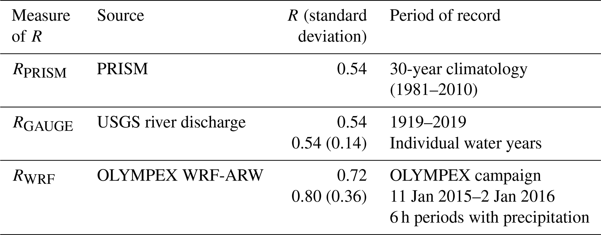
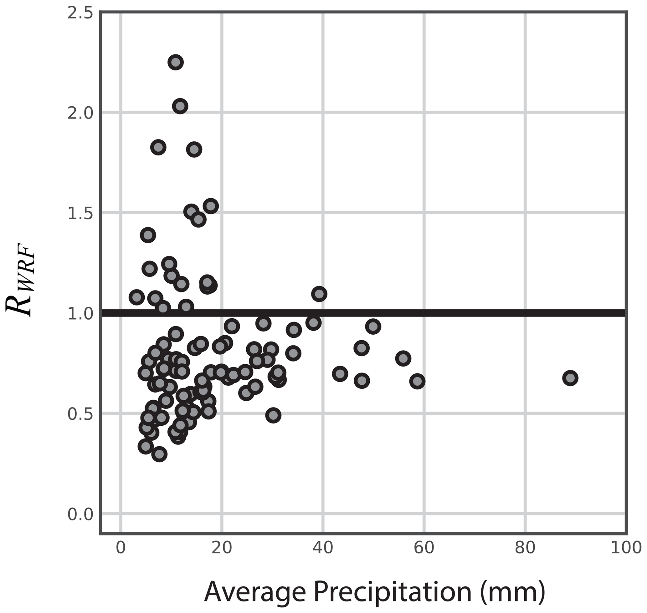
Figure 2 R_WRF measured at 6 h intervals varies with the total precipitation averaged over the two basins. As the average precipitation increases, R_WRF becomes less variable.

R_WRF for the entire OLYMPEX campaign equals 0.72 (Table 1; Eq. 3; Fig. 2). An R value closer to one means precipitation is more similar in the Quinault and Elwha. WRF forecasts predicted significantly larger amounts of spillover precipitation in the Elwha basin than the PRISM dataset. However, the WRF forecasts are imperfect. WRF underestimated the precipitation by up to 100 mm at OLYMPEX gauge locations around the Quinault basin during larger storms (Conrick and Mass, 2019b). Additionally, the OLYMPEX campaign only studied a single wet season, which may not have been representative of longer-term average precipitation.

A 101-year river discharge of the Elwha and Quinault basins yielded R_GAUGE=0.54 (Eq. 5; Table 1), which is in agreement with R_PRISM. Uncertainty in the discharge measurements and hence R_GAUGE can stem from several sources. For example, there is uncertainty in the measurements of the cross-sectional area of the flow and in the stage–discharge relationship. Additionally, river discharge represents water flowing off the land surface, neglecting the possibility of the evapotranspiration of precipitation. This could result in an underestimation of the actual amount of precipitation that contributes to the river discharge measurements. The cool, wet climate of the Olympic Peninsula makes this error likely to be relatively small, but there could be systematic differences between the Quinault and Elwha in the conversion of precipitation to river discharge.

2.2.2 Temporal variability in rain shadow strength

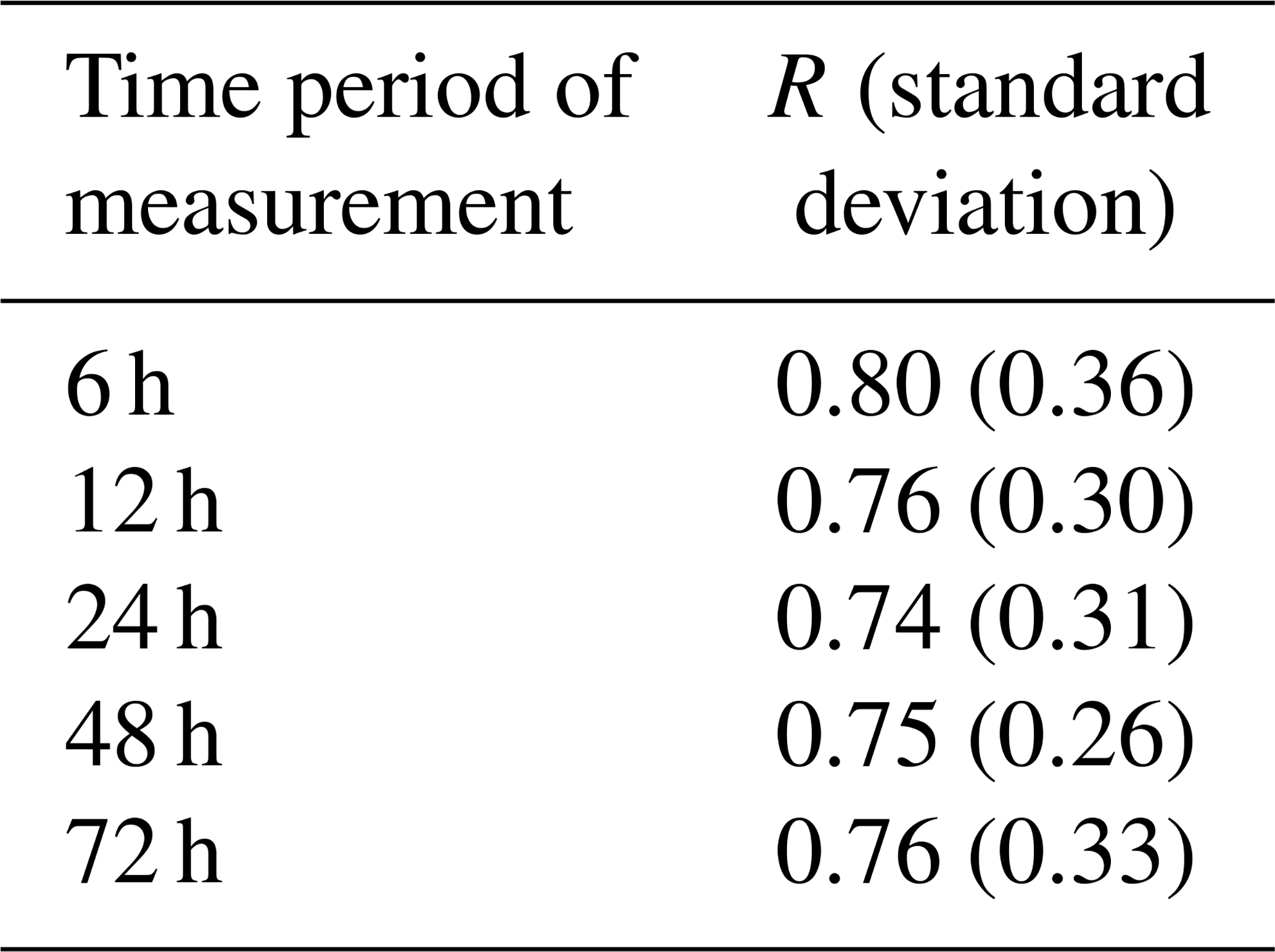
In addition to the average rain shadow indices estimated using these three independent datasets, we also considered the variability in the rain shadow index at timescales of hours and seasons. The 6 h R_WRF values have a mean of 0.80 and standard deviation of 0.36 (Table 1). The mean rain shadow index measured in this way is larger than the OLYMPEX total R_WRF (=0.72), meaning that the 6 h forecast precipitation is more uniform across the mountain range than other datasets. We note that at a 6 h resolution, it is possible that the measured rain shadow index could reflect differences in the timing of precipitation in the two basins. For example, if the heaviest precipitation in the Elwha occurs after it happens in the Quinault, then the rain shadow index might be larger in one 6 h period and smaller in the subsequent 6 h period, with neither measure reflecting the storm event. Therefore, we averaged WRF forecasts over longer time periods to produce time series of R over a range of timescales. Over longer time periods, the mean value for R and the standard deviation of R becomes smaller up to 48 h (Table 2). For the longest time period examined, 72 h, the standard deviation increases relative to 48 h, possibly reflecting less coherence in the conditions at these longest timescales. For all timescales examined, however, R derived from WRF forecasts during OLYMPEX is larger than in other datasets. The larger R may reflect a tendency of WRF to overpredict spillover precipitation in the Elwha basin. However, we do not have sufficient data to conclude that this is necessarily the case. Moreover, PRISM is not informed by data collected near the drainage divide and so is not necessarily reliable. Similarly, R estimated from differences in river discharge is complicated by the existence of the difference in evapotranspiration between the basins, if this is the case. Finally, it is possible that the OLYMPEX period was anomalous when compared with longer-term records.

Table 2 Mean and standard deviation of R_WRF at different time intervals for accumulated precipitation.

What causes the time variability in the 6 h R_WRF? Figure 2 compares the 6 h R_WRF to the average amount of precipitation. It shows that the rain shadow strength for large events is less variable than for all rain events. Specifically, 6 h periods with average precipitation totals above 20 mm tend to cluster at R values between 0.5 and 1.0, indicating that higher values of 6 h R_WRF are generally associated with lighter precipitation.

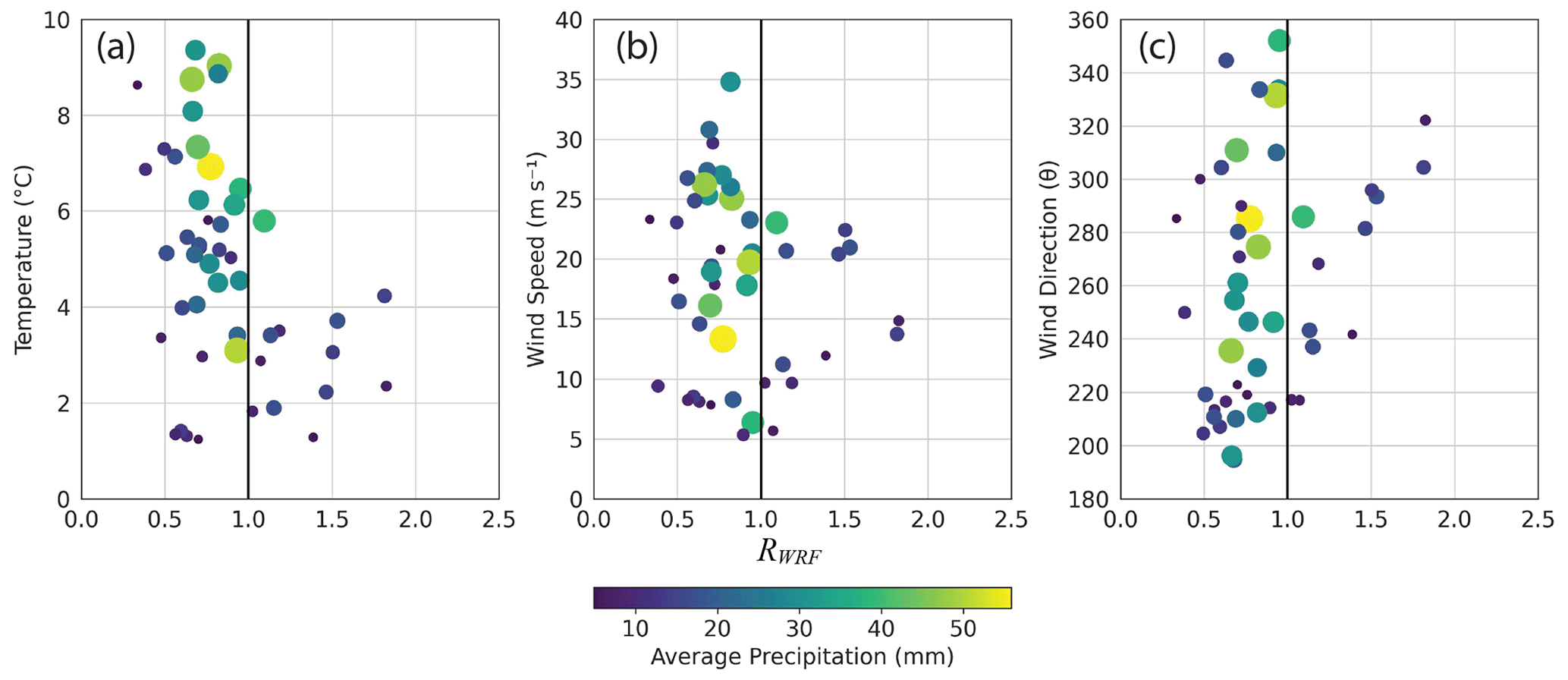
Figure 3 The relationship between R_WRF at 6 h resolution and atmospheric variables as measured by the KUIL radiosonde. Panel (a) shows the average temperature between 750 and 1750 m a.s.l. Panel (b) shows the average wind speed over the same elevation range. Panel (c) shows the average wind direction in the same elevation range. The size and color of the data points correspond to the average precipitation across both basins.

We analyzed the time series of 6 h R_WRF to examine the relationships between R magnitude and temperature, wind speed, and wind direction (as measured by atmospheric soundings; Fig. 3). The time series can be divided into groups of low (0.34–0.69), moderate (0.70–0.99), and high (1.0–2.5) R. High R values (greater than one) were commonly observed during colder weather conditions (Fig. 3a). On the other hand, lower R values were associated with higher temperatures. High R events had lower-magnitude precipitation compared to moderate R events, with rates of approximately 14 mm per 6 h interval and 26 mm per 6 h interval, respectively. The wind speed during cold, high R events was lower compared to low and moderate R events (Fig. 3b), while wind direction showed no significant pattern among the different R groups (Fig. 3c). In general, the temporal variability in R_WRF suggests that colder conditions and slower winds lead to lower-magnitude and more uniform precipitation, while warmer and windier conditions are linked to R values close to the long-term average. Small-magnitude precipitation events with R values below 0.5 occurred during warm and windy conditions.

We used discharge records to examine differences in rain shadow strength in different water years. The annual time series of R_GAUGE has a mean value of 0.54, with a standard deviation of 0.14 (Table 1). We compared the time series of R_GAUGE, E_run, and Q_run to climate indices to determine if the temporal variability in R is correlated with specific climate patterns, for example, La Niña vs. El Niño. Instead, we find that there is a remarkably consistent relationship between Q_run and E_run (r=0.98), and the climate indices do not strongly correlate with E_run, Q_run, or R_GAUGE (Fig. 4). Our analysis demonstrates that river discharge varies synchronously on the windward and leeward sides of the mountain range. This suggests that topography, and possibly differences in evapotranspiration, strongly influence the rain shadow strength at the timescale of entire wet seasons.

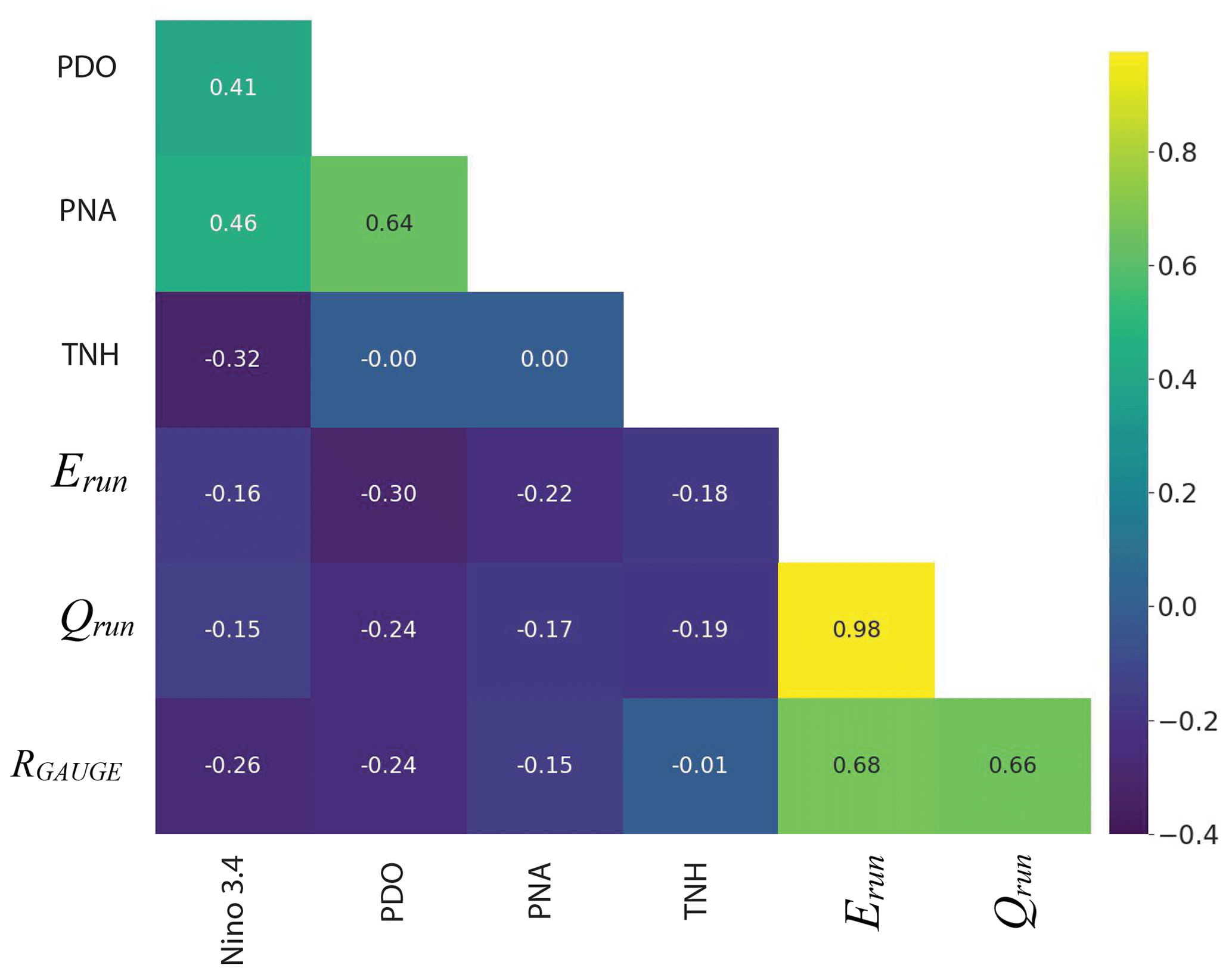
Figure 4 A correlation heat map displaying the relationship between climate indices for the El Niño–Southern Oscillation (Niño 3.4, 2022), the Pacific Decadal Oscillation (PDO, 2022), the Pacific North American Pattern (PNA, 2022), and the tropical Northern Hemisphere Pattern (TNH, 2022) and E_run, Q_run, and R_GAUGE. E_run and Q_run are highly correlated with each other, and R_GAUGE is not correlated with climate indices.

2.3 Inferences for reconstruction of past climate

Three independent datasets give us R of ∼0.5 to ∼0.7, with less variability in R at longer timescales. At the shortest timescales examined (6 h), the largest deviations in R are values larger than 1 occurring during periods of cold, slow wind speeds, and light precipitation. There is no example of a large precipitation event, with R being much less than 0.5 during the OLYMPEX campaign. At the timescale of water years, R is uncorrelated with regional climate indices, and the river discharge varies synchronously between the Quinault and Elwha basins. The lack of variability in R at the water year timescale, the lack of correlation of R with climate indices, and the small number and magnitude of low R events at the 6 h timescale all suggest that a conservative minimum estimate of R in the Olympic Mountains during the last glacial period is 0.5. The most likely difference between the modern and glacial climate suggested by our data would be an increase in R (i.e., a more uniform climate) due to cooler conditions (Fig. 3). We proceed, therefore, to explore how the current rain shadow strength would have impacted glacier dynamics on the Olympic Peninsula.

3 Modeled glacier extent in the Quinault and Elwha basins

3.1 Glacier flowline model methods

We use a flowline model based on that of Oerlemans (1997), adapted from Roe and O'Neal (2009), to approximate the dynamics of glaciers in the Quinault and Elwha valleys. The model is one-dimensional but includes the effect of changes in the valley width when considering mass conservation along the flowline. We follow the work of Roe and O'Neal (2009) by calculating the mass balance along the flowline as a function of precipitation and temperature instead of imposing a specified vertical mass balance gradient. Inputs to the model include valley geometry, initial ice thickness, sea level temperature, atmospheric lapse rate, and precipitation rate. The horizontal grid spacing in the model is 500 m.

Valley geometry is idealized as a long profile with a valley floor of a defined width and valley sidewalls sloping outward at a fixed angle above the valley floor. The Quinault and Elwha valleys have different morphology and hypsometry (Fig. 5), which is likely to affect glacier dynamics. For simplicity, the geometry of each valley was idealized using three segments with uniform width and the valley angles for each segment, with the valley floor elevation defined by the elevation of the lowest part of the valley extracted from a 30 m digital elevation model (Table 3). We make no attempt to remove glacial and post-glacial sediment from the valleys before extracting the long profile. Where the valleys are wide, the valley side walls are assumed to be vertical. Within narrow sections, we define the angle at which valley walls slope outward. Both valleys start with a wide contributing area in the high headwaters. In the middle of each basin, there is a narrow notch. Below the notches, the basins open into expansive coastal plains. Basin widths were chosen to approximate the upstream area accumulation along the long profile.

Table 3 Elwha and Quinault valley geometry parameterization for the one-dimensional flowline model.

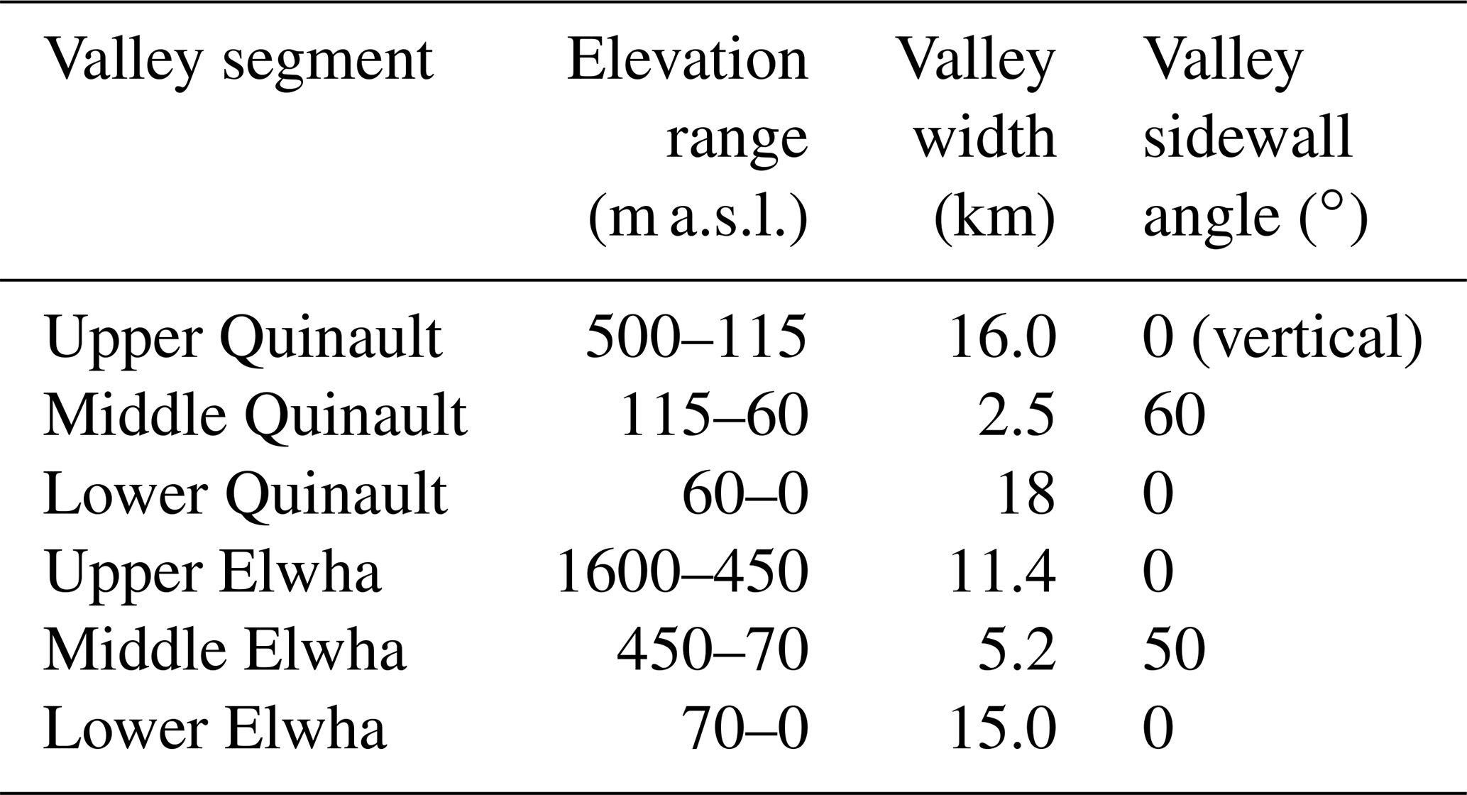
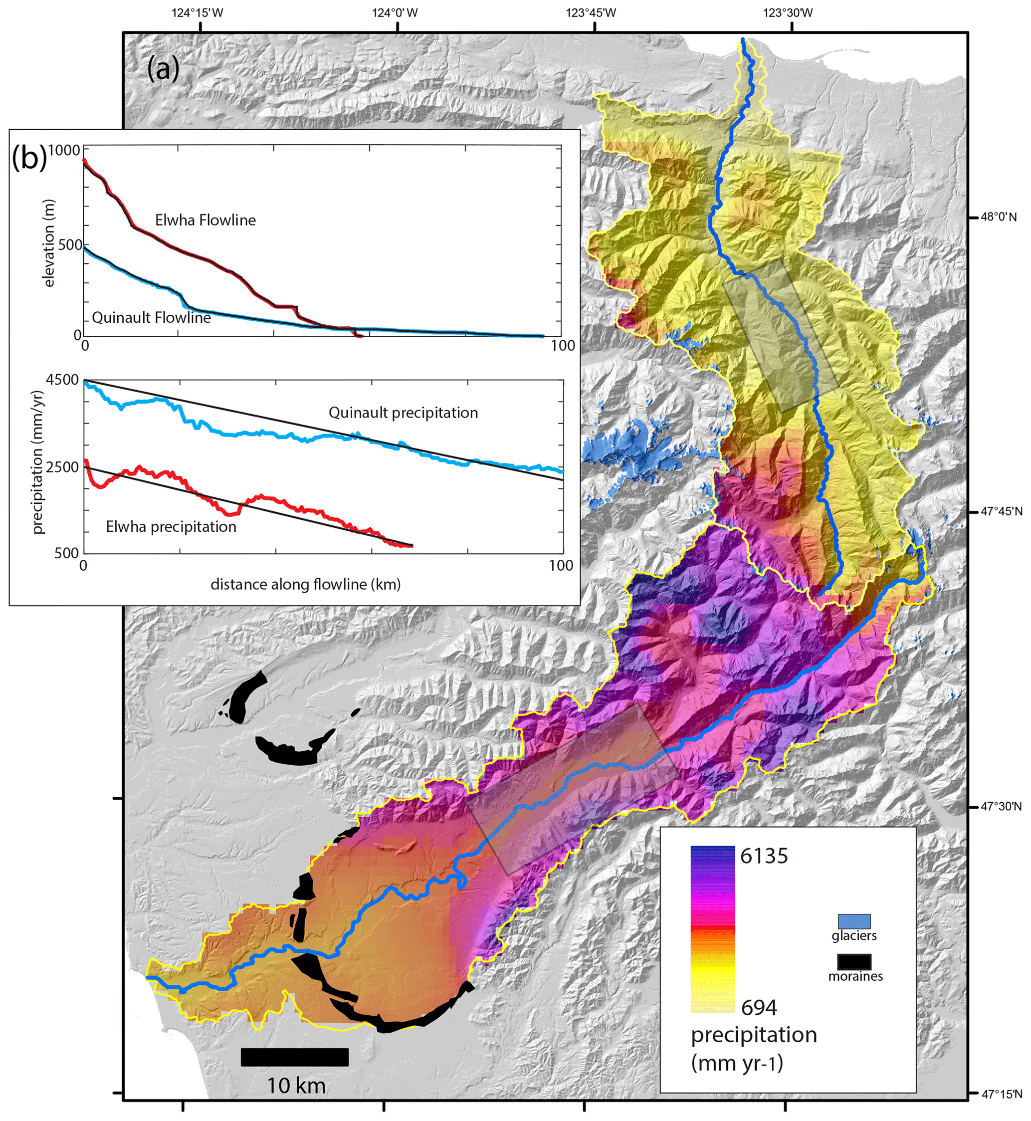
Figure 5 Panel (a) shows the Quinault and Elwha valleys, with the topography represented as a gray hillshade and the 30-year climatological annual precipitation (in mm yr⁻¹) shown by the color bar. Blue lines trace the path of the flowlines modeled. Boxes with gray shading are regions where the valleys narrow. Modern glaciers are indicated by blue shading, and the past glacier extent moraines are in black. Panel (b) shows the elevation and precipitation along the flowlines, with the colored lines showing the data from the digital elevation model (DEM) and PRISM (2020) model and the black lines showing the approximate values used in our model.

The mass balance of the glacier varies along its length as a function of spatially variable precipitation and summer mean temperature. Summer temperature (T) varies along the length of the flowline (x) and is a function of elevation of the ice surface and an imposed sea level temperature, T_SL, as follows:

$$\begin{array}{}\text{(3)}& T\left(x\right)=T_{\mathrm{SL}}+\mathit{\gamma }\left(zb\right(x)+h(x\left)\right),\end{array}$$

where γ is the atmospheric lapse rate, here chosen as $-\mathrm{8.5}\times {\mathrm{10}}^{-\mathrm{3}}$^∘C km⁻¹, zb(x) is the elevation of the bed, and h(x) is the thickness of the ice. Precipitation decreases down-valley in both basins and is generally lower in the Elwha basin (Fig. 5). We idealize this variability by setting a precipitation rate at the top of the basin and imposing a fixed fractional decrease in the precipitation from the top to the bottom of each valley. For the Elwha valley, we assume that the precipitation at the valley mouth is 27 % of that of the valley top. For the Quinault valley, we assume that the precipitation at the valley mouth is 44 % of that at the valley top. These fractions were chosen to approximate the modern spatial pattern in precipitation (Fig. 5). To simulate a glacial climate, we make the climate drier than modern by imposing a glacial drying factor (GDF) of less than 1. The idealized modern precipitation gradient is multiplied by the GDF to model a drier climate that maintains the down-valley precipitation gradient observed today. We compare the modeled glaciation of the Elwha and Quinault basins with the same T_SL and GDF to assess the response of the different basins to the same climate forcing.

Modeled temperature and precipitation are used to calculate the mass balance along the flowline. Precipitation is assumed to be adding mass throughout time and across the entire glacier surface. Temperature-dependent melting is assumed to be the only loss of mass and is calculated as

$$\begin{array}{}\text{(4)}& \mathrm{melt}\left(x\right)=\mathrm{maximum}(\mathrm{0},\mathit{\mu }T(x\left)\right),\end{array}$$

where μ is a constant melt factor set to 0.65 m yr^−1 ∘C⁻¹, following the work by Roe and O'Neal (2009) on Mount Baker in the neighboring Cascade Range. From this, we calculate a spatially variable mass balance, b(x) (in m yr⁻¹), as

$$\begin{array}{}\text{(5)}& b\left(x\right)=P\left(x\right)-\mathrm{melt}\left(x\right).\end{array}$$

With the mass balance calculated, we follow the method of Oerlemans (1997), as implemented by Roe and O'Neal (2009) and Stuart-Smith et al. (2021), to solve the nonlinear diffusion equation governing the height of the ice over time. We choose a fixed value of $\mathrm{1.9}\times {\mathrm{10}}^{-\mathrm{24}}$ Pa⁻³ s⁻¹ as the parameter controlling the internal deformation and $\mathrm{5.7}\times {\mathrm{10}}^{-\mathrm{20}}$ Pa⁻³ m² s⁻¹ as the sliding parameter, based on values used in Oerlemans (1997), which are based on Budd et al. (1979). The model requires ice to be present at the beginning of simulations. Therefore, we start with glaciers of the expected scale and use a large glacier near the terminal moraine for the initial condition for the Quinault valley and use a small initial glacier limited to the headwaters in the Elwha valley. The model is implemented in MATLAB, and the model code and basin geometry input files are publicly available at https://doi.org/10.4211/hs.fe28143081434b0d90f8cffc88e1bfff (Margason, 2023a).

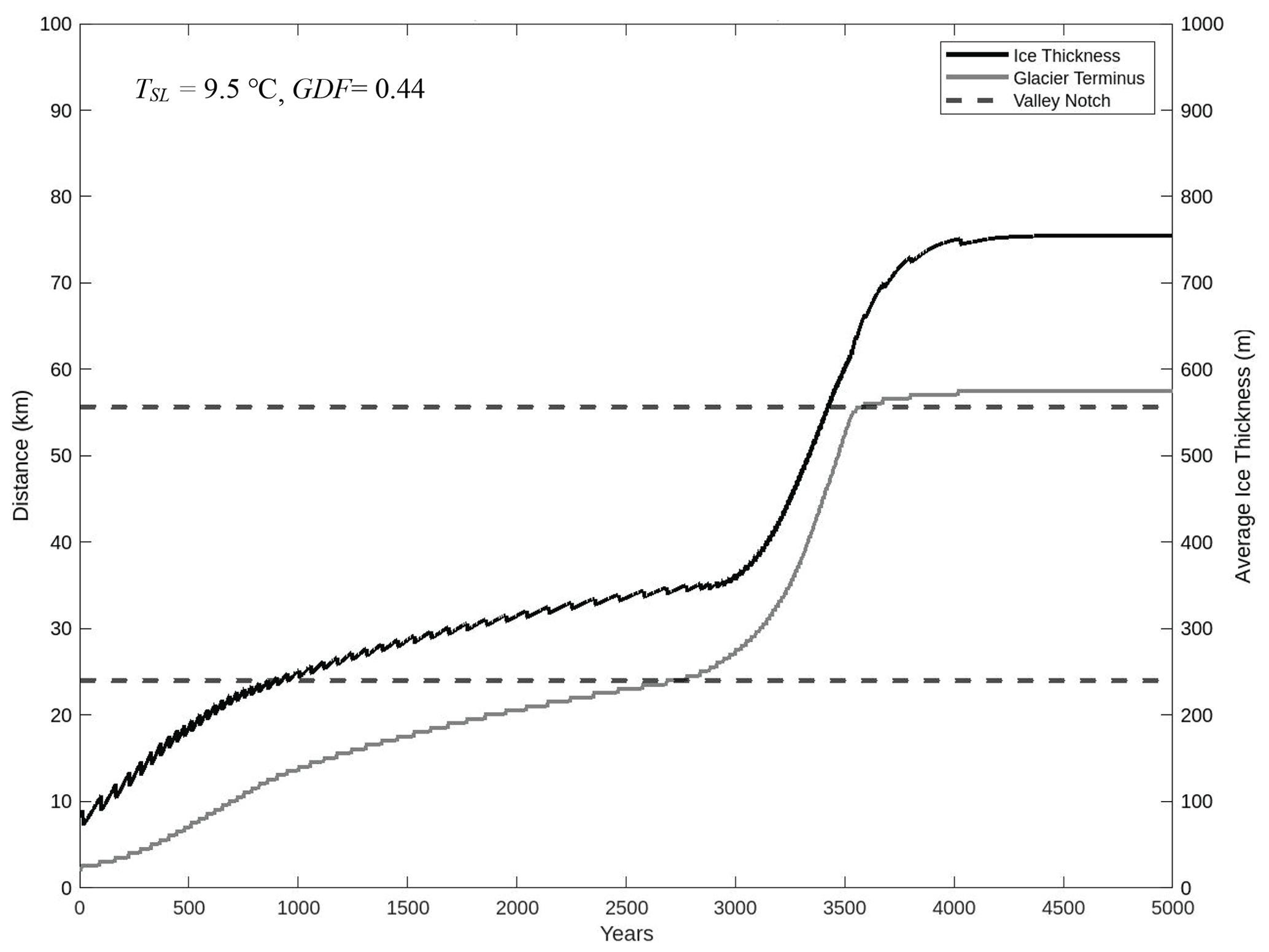
Figure 6 The temporal evolution of the Elwha glacier terminus and ice thickness for T_SL=9.5^∘ and GDF = 0.44. These climate factors yield an equilibrium Quinault glacier at its terminal moraine position. As the Elwha glacier terminus (gray line) advances into the narrow section of the valley (distance of approximately 23 to 56 km, as shown on the left axis) just before 3000 years into the simulation, the ice thickness (black line) increases rapidly, initiating an ice elevation feedback. Upon reaching the other side of the valley notch, the glacier reaches a state of equilibrium, where the rates of accumulation and ablation are roughly equal. It is important to note that this ice elevation feedback is not observed in all climate simulations but is more likely to occur in cooler and drier conditions and in basins with valley geometries similar to that of Elwha.

3.2 Results of glacier flowline modeling

We begin by finding the range of climate conditions that produce a modeled Quinault glacier in equilibrium at the observed Early Wisconsin maximum extent (Fig. 1b). Using a trial-and-error approach, we identify pairs of T_SL and glacial drying factor (GDF) that produce an equilibrium glacier at the terminal moraine. T_SL and GDF linearly trade-off (GDF = 0.10 T_SL − 0.55) within the range of sea level temperatures between 7 and 11 ^∘C supported by paleoclimate reconstructions (Heusser et al., 1999). For a chosen value of T_SL, we can find the percentage of precipitation (GDF) that forces the glacier to stay in equilibrium near its terminal moraines over a 5000-year period. Encouragingly, the corresponding GDF values (∼0.15–0.55) are similar to the required drying of at least 0.33 implied by the paleoclimate record.

Having found equilibria for the Quinault glacier, we use the same climate T_SL and GDF pairs to simulate the evolution of the Elwha glacier. Pairs of climate variables that produced nearly identical equilibrium glaciers in the Quinault led to enormously different glaciers in the Elwha valley. At the hotter end of the climate range at 10.5 ^∘C, the Elwha glacier reaches a steady state with a high-elevation terminus consistent with the most likely true behavior of the Elwha glacier during the most recent glaciation. However, for a cooler climate at 9.5 ^∘C, the Elwha glacier advances far down-valley onto the coastal plain (Fig. 6). The Elwha glacier advances from the headwaters into the narrower portion of the valley, which is about 25 km from the divide. The glacier thickens due to the abrupt change in cross-sectional area. The thickening causes the surface of the ice to be at higher elevations. This increases the accumulation area of the glacier. A larger accumulation area causes glacier growth and further increases in glacier elevation. The sensitivity of the feedback loop between ice elevation and glacier growth to climate conditions is pronounced for the Elwha glacier, despite the range of climate conditions being similar to those that result in little change to the Quinault glacier. As a result, even slight alterations in climate conditions can produce significant contrasts in the behavior of the Elwha glacier in comparison to the Quinault glacier.

3.3 Discussion of flowline model results

Our findings indicate that the Elwha glacier model experiences an ice elevation feedback that is associated with the geometry of the basin. The initiation of the feedback occurs when the glacier advances into the narrow section of the valley (notch), where it begins to thicken (Fig. 6). The Quinault valley also has a narrow segment in the middle of the basin; therefore, we expect to see the occurrence of a similar ice elevation feedback in this valley. To investigate this possibility, we ran a set of models with an initially small Quinault glacier. In some simulations, this glacier grew large enough to advance through the narrowing of the valley. It thickened and extended, demonstrating an ice elevation feedback that is similar to what we observed in the Elwha simulations.

The geometry of the basins is not the only control on the glacier extent. We ran a set of simulations switching the basin geometry. That is, we ran the Quinault climate over the Elwha valley geometry, and vice versa. The Elwha glacier was consistently large when given Quinault precipitation rates. The Quinault glacier ablated away or grew large when given the Elwha precipitation rates. This indicates that the contrast in precipitation amount, rather that the valley morphology, is the main cause of the different extent of the Quinault glacier and Elwha glacier in our models. This finding also suggests that if precipitation gradients were weaker in the past, then they would not be sufficient to explain the observed difference in glacier extent.

Assuming that the geologic mapping of the Elwha valley has correctly identified the limited extent of recent glaciation, we can interpret our results as demonstrating that precipitation gradients are sufficient to explain differences in glacier extent if the past climate was at the warm and wet end of the range of paleoclimate estimates. However, the valley geometry and sensitivity of the Elwha glacier to climate variability within a plausible range suggests that the possibility of the large-scale glaciation of the valley during the Quaternary should be considered.

In our model, we have neglected other spatially variable surface processes that could have influenced the extent of the Elwha glacier. Specifically, we did not account for the separate influences that precipitation type, cloudiness, humidity, and sublimation would have on glacier accumulation and melt. In the model, we did not discriminate between different types of precipitation. All precipitation was considered snow. Rain will not contribute to glacier mass gain. If a significant portion of the precipitation falls as rain, then we are overestimating accumulation. We expect that the majority of the precipitation during the Early Wisconsin is snow because we expect a seasonal shift in temperature that is similar to the present, which brings winter temperatures at sea level to within a few degrees of freezing, and about 80 % of modern precipitation is during the cool season. However, at the lowest elevations and during the warm season, rain likely occurred during the Early Wisconsin glacial advance. The larger precipitation totals in the Quinault suggest that this effect could be more important for this glacier than for the Elwha. Cloudiness modulates the amount of solar radiation that reaches a glacier's surface. We expect that the same physics that creates the rain shadow should produce coherent spatial patterns in cloudiness in the Olympic Mountains. Clouds form on the windward side of the range due to orographic lifting and then dissipate when they descend on the leeward side of the mountain range (Roe, 2005). During some precipitation events, clouds are observed to decrease in elevation and water content rapidly near the divide between the Quinault and Elwha valleys (Zagrodnik et al., 2019). If the Elwha valley is less cloudy than the Quinault valley, then we expect that more solar radiation would increase local air temperatures and enhance glacier melt (Huss et al., 2009). Additionally, there could be spatial patterns in humidity that influence glacier mass balance. If the Elwha valley is systematically less humid, we expect that the lapse rate should be larger than in the wetter Quinault valley. Descending airflow in the lee of the mountain range could decrease humidity and increase lapse rate in the Elwha valley relative to the Quinault.

We conducted a small number of experiments to determine the sensitivity of the modeled Elwha glacier to our choice for the melt factor. For the simulation shown in Fig. 6, if we increase the melt factor slightly from 0.65 to 0.75 m yr^−1 ∘C⁻¹, then the Elwha glacier remains small. The melt factor for the Blue Glacier, on the west side of the Olympic Mountains, was estimated using the glacier area change and PRISM-based temperature and precipitation data (Fountain et al., 2022). Field measurements could constrain the melt factor in the eastern Olympic Mountains to assess the potential for enhanced melt in the Elwha basin relative to the Quinault. Future work could establish if climatological variability in cloudiness is equivalent to this degree of difference in the melt factor relative to the Quinault basin. The role of lapse rate variability could also be explored. Additionally, a more sophisticated glacier model could be used for two-dimensional simulations that would depict the valley geometry more specifically and include two-dimensional spatial variability in precipitation and aspect-related melting. Our flowline model captures the variability in the direction of the steepest precipitation gradients but neglects variability across the valleys that may be important, especially for spatially variable drivers of ablation, such as topographic shading.

Although we defend our analysis of the modern climate and our reasonable assumption that the past spatial gradient in precipitation in the Olympic Mountains was similar to that observed today, it is important to acknowledge that precipitation events during the last glacial period may not have any modern climate analogues. One way to assess this possibility would be to use a forecasting model like WRF, with boundary conditions pulled from global circulation models of the Early Wisconsin. These simulations could reveal different mechanisms of precipitation variability than those that operate today.

Any assessment of erosion by glaciers on the Olympic Peninsula requires a clear picture of the glacier extent through time. To model glacial erosion in the Quinault valley, we should simulate the advance and retreat of the Quinault glacier through a glacial cycle and integrating basal sliding. The spatial pattern of glacier sliding within the Quinault valley could be compared to gradients in exhumation across the range and fluvial erosion within the Clearwater Valley. Glacial erosion of the Elwha valley depends on the extent of ice. If the Elwha glacier remained small during the last glacial episode, then glacial erosion was limited, and perhaps fluvial erosion was a stronger control on landscape-scale erosion on the lee side of the range. However, if an expansive and thick glacier ever occupied the Elwha valley, then our models suggest that it was very fast flowing and erosive – more so than the Quinault glacier.

Future fieldwork could improve our understanding of the past extent of the Elwha glacier. One target would be to find terminal moraines associated with the Elwha valley glacier during the most recent glaciation, presumably located up-valley from the mapped quadrangles near the valley mouth. If these are above the notch, then they would improve our confidence in the model simulations. In the lower Elwha valley, drill cores could be recovered and analyzed to identify the extent of locally derived (alpine) till. It is possible that alpine till from previous glaciations could be identified from the mineralogy and chemistry, allowing us to constrain the past glacier extent.

4 Conclusions

We set out to understand the factors influencing the asymmetry in the glacier extent between the Quinault and Elwha valleys of the Olympic Mountains. To this end, we characterized the modern precipitation patterns and assessed the potential influence of various climate indices on these patterns. We calculated ratios of average precipitation in the Elwha basin relative to the Quinault basin using three different datasets, namely PRISM (2020) data, river discharge data (USGS 2022a, 2022b), and WRF model output. We conclude that the long-term ratio of average precipitation between the two basins likely remained at or above 0.50 (<100 % more precipitation in the Quinault than the Elwha) during recent glaciations. We find no evidence of atmospheric or climatic influences, such as weather regimes, that would cause a more severe precipitation gradient in a glacial climate. Therefore, we make the conservative assumption that the modern climate is a good representation of past spatial gradients in precipitation.

To better understand the response of glaciers in the region to climate, we employed a one-dimensional glacier flowline model simulating the response of glaciers in both valleys to a range of climate states. This included variations in sea level temperature (T_SL) and the glacial drying factor (GDF). There exist a set of T_SL and GDF pairs within the expected paleoclimate range that produce an equilibrium ice margin in the Quinault valley at the position of the local Last Glacial Maximum terminal moraine. Over this same set of climate conditions, the Elwha glacier showed extremely variable behavior. Within the Quinault equilibrium climate range, a 1 ^∘C change in temperature corresponded to an expansion of nearly 40 km in the Elwha glacier. Further investigation revealed that this behavior was related to the valley geometry of the Elwha valley, with the glacier experiencing an ice elevation feedback as it advanced into the narrowing section of the valley and thickened. This ice elevation feedback occurs in both the Quinault and Elwha valleys but is more pronounced in cooler and drier climates. In general, our model was able to reproduce the observed extent of glaciers in warmer climates with higher rates of precipitation. The occurrence of an ice elevation feedback in both valleys, which was linked to the valley geometry, highlights the importance of considering local topography in studies of glacier dynamics.

Our model focused on glacier asymmetry due to the asymmetry in the precipitation and did not consider the differences in the efficiency of melting across the Olympic Mountains. Our parameter tests suggest that if the melt efficiency was even slightly greater in the Elwha valley relative to the Quinault valley, then it could have been a significant factor limiting the growth of the Elwha glacier during the last glacial episode. Further investigation with the flowline model could examine the impact of spatial variability in glacier melting.

Overall, we find that spatially variable precipitation influences the extent of glaciers and that the sensitivity of glaciers to climate varies in space within the Olympic Mountains. This conclusion has implications for other regions with spatial gradients in precipitation including the Andes Mountains, the European Alps, the Southern Alps, and Central Asia. Specifically, we suggest that glacier sensitivity to climate likely varies across precipitation gradients forced by topography. Furthermore, the local spatial variability in the relationship between glaciers and climate complicates predictions of the response of glaciers to ongoing anthropogenic climate change, as small changes in climate may have different impacts for different glaciers within the same mountain range. Considering the complex interplay between local topography and climate, it is necessary to take into account these spatial gradients in future climate projections for accurate predictions of individual glacier behavior in mountainous regions.