Sediment source and sink identification using Sentinel-2 and a small network of turbidimeters on the Vjosa River

Measurement of suspended sediment concentration (SSC) at a basin outlet yields a basin-integrated picture of sediment fluxes; however, it does not give a full spatial perspective on possible sediment pathways within the catchment. Spatially resolved estimates of SSC along river networks are needed to identify sediment sources and sinks, to track erosion gradients, and quantify anthropogenic effects on catchment-scale sediment production, e.g., by dam construction or erosion control. Here we explore the use of high-resolution Sentinel-2 satellite images for this purpose in narrow and morphologically complex mountain rivers, combined with ground station turbidity sensing for calibration and supported by a Lagrangian kayak-derived river profile measurement. The study is carried out on the Vjosa River in Albania, which is one of the last intact large river systems in Europe. We developed a workflow to estimate river turbidity profiles from Sentinel-2 images including atmospheric, cloud cover, and deepwater corrections for the period May 2019 to July 2021 (106 images). In situ turbidity measurements from four turbidity sensors located along the Vjosa River provided ground truthing. A multivariate linear regression model between turbidity and reflectance was fitted to this data. The extracted longitudinal river turbidity profiles were qualitatively validated with two descents of the river with a turbidity sensor attached to a kayak. The satellite-derived river profiles revealed variability in turbidity along the main stem with a strong seasonal signal, with the highest mean turbidity in winter along the entire length of the river. Most importantly, sediment sources and sinks could be identified and quantified from the river turbidity profiles, both for tributaries and within the reaches of the Vjosa. The river basin and network acted as a sediment source most of the time and significant sediment sinks were rare. Sediment sources were mostly tributaries following basin-wide rainfall, but within-reach sources in river beds and banks were also possible. Finally, we used the data to estimate the mean annual fine sediment yield at Dorez at $\sim \mathrm{2.5}\pm \mathrm{0.6}$ Mt yr⁻¹, in line with previous studies, which reveals the importance of the Vjosa River as an important sediment source of the Adriatic Sea. This work presents a proof of concept that open-access high-resolution satellite data have potential for suspended sediment quantification not only in large waterbodies but also in smaller rivers. The potential applications are many, including identifying erosion hotspots, sediment activation processes, local point sources, glacial sediment inputs, and sediment fluxes in river deltas, with a necessary future research focus on improving accuracy and reducing uncertainty in such analyses.

1 Introduction

The transfer of sediment from land to oceans plays an important role in the global denudational cycle (Gregor, 1970; Wold and Hay, 1990), global biogeochemical cycles (Meybeck, 1994; Ludwig et al., 1996; Sanders et al., 2014), the functioning of riverine and coastal ecosystems (Roy et al., 2001; Arrigo et al., 2008; Terhaar et al., 2021; Descloux et al., 2013), and the evolution of rivers, deltas, and other coastal landforms (Morton, 2003; McLaughlin et al., 2003; Seybold et al., 2009). Present-day sediment export from the land surface to global oceans by large rivers is estimated at about 15.5–18.5 Gt yr⁻¹, and the dominant part of this flux is fine grain transport by wash load and suspended load (Peucker-Ehrenbrink, 2009; Syvitski and Kettner, 2011; Cohen et al., 2022). This is about half of the estimated global annual soil erosion from the land surface (Borrelli et al., 2017). Excessive amounts of fine sediment load in rivers lead to high water turbidity, which can be linked to the degradation of coral reefs (Brown et al., 2017), impairment of freshwater and marine fish populations (Kemp et al., 2011; Newport et al., 2021; Jensen et al., 2009), the clogging of riverbeds in gravel bed streams (Schälchli, 1992; Hauer et al., 2019b), and low water quality in general. However, riverine suspended sediments provide an important balance of nutrients (phosphorous, nitrogen, and silica) to the coast and ocean (Nixon et al., 1996; Bernard et al., 2011). In addition, recent silica deficiency due to the reduction in suspended sediment inputs from river damming has been observed to exacerbate eutrophication by reducing the role of diatoms in coastal food-webs, which indirectly feeds mesozooplankton (copepods; Cotrim da Cunha et al., 2007; Justić et al., 1995).

Although recent studies point to the importance of large rivers in the overall global sediment flux (Cohen et al., 2022), there is an increasing understanding that smaller mountainous rivers, with basin areas less than 10 000 km² and draining elevations higher than 1000 m, deliver disproportionately more sediment per unit drainage area than large rivers. These smaller mountainous basins rich in sediment sources cover only about 10 % of the land area draining into global oceans but account for about 15 % of the annual water discharge and 45 % of the annual suspended solids reaching the oceans (Milliman and Farnsworth, 2013). Smaller rivers are also more likely to be subject to human disturbance, either by trapping sediment behind dams or by increased sediment inputs due to agriculture, mining, and intensive land-use (Syvitski et al., 2022). In fact, in Europe, there are very few unregulated moderately sized rivers where natural fine sediment dynamics can be monitored and studied. In addition, it is estimated that over 1 million instream barriers fragment European rivers (Belletti et al., 2020).

This is also the case with the three largest rivers draining into the Adriatic Sea (Po, Adige, and Drini) which would have accounted for 25 % of the sediment discharged to the Adriatic prior to dam construction. The remaining 75 % of the Adriatic’s sediment input comes from 32 rivers, their drainage basins all being less than 7000 km² (Milliman et al., 2016). Prior to dam construction, Albanian rivers contributed about 60 % of the total sediment entering the Adriatic (Milliman et al., 2016), with the Vjosa River discharging more than 8.3 Mt yr⁻¹ and with suspended load accounting for 80 %–85 % of this flux or 6.6–7.1 Mt yr⁻¹ (Ciavola, 1999). In addition to its importance as a sediment source, the Vjosa River represents one of the last intact large river systems in Europe. Although the headwaters are dammed (potentially reducing the residual flow of the river) and there is one hydropower dam along one of the Vjosa tributaries (sediment source), the Vjosa features a largely unobstructed fluvial morphology over the entire river corridor. Its geological diversity and longitudinal continuity in water flow and sediment transport processes from its headwaters to the Adriatic Sea represent an important reference system for dynamic floodplains that have already been lost all across Central Europe (Schiemer et al., 2018b). Due to the largely undisturbed catchment and high surface runoff production, where about 70 % of the total river flow is estimated to come from surface runoff following rainfall (Hauer et al., 2021), fine sediment is regularly mobilized on hillslopes and in the channels, giving rise to a natural sediment regime with many sources and sinks within the river network.

Despite the importance of fine sediment fluxes in rivers such as the Vjosa, the monitoring of sediment concentrations for estimating sediment yields from river basins is extremely difficult when compared to hydrological monitoring of river stage and discharge. There are basically three different options available: (a) direct measurement of suspended sediment concentration (SSC) in streams by periodic water sampling, (b) continuous measurement of turbidity by permanently installed sensors and estimation of SSC, and (c) estimation of SSC based on measurements of water surface reflectance by calibrated remote optical sensors (satellites, UAVs). In order to identify sediment sources and sinks along a river network, and not just sediment yields at the outlet, we would need to monitor SSC at many points upstream and downstream of tributaries and other local sources. The first two options, i.e., direct SSC measurements and in situ measurements of turbidity would be impractical for this purpose because a large network of turbidity sensors or intensive SSC sampling would be needed. This is very labour intensive and costly, also because of a lack of cheap alternatives for turbidity sensing (Gillett and Marchiori, 2019). The third option with remote sensing of turbidity using satellite imagery has higher potential as it is distributed in space, repeatable, and affordable, despite being less accurate.

Turbidity monitoring by remote sensing is based on the reflectance of the water surface. The intrinsic colour of natural waters is determined by a range of parameters such as the concentrations of dissolved and suspended matter together with gross biological activity (e.g., chlorophyll, suspended sediment, and coloured dissolved organic matter; e.g., Novoa et al., 2015; Wang et al., 2018; Ritchie et al., 2003). These components affect water surface reflectance in a predictable way, which makes optical satellite remote sensing of oceans, coastal areas, and large lakes/rivers possible. Satellite imagery with multispectral ranges is even more useful for a range of water quality parameters (e.g., Wang and Sohn, 2018). Several studies have investigated the plausibility of relating the remotely sensed reflectance signals from large waterbodies with in situ turbidity or SSC measurements (Doxaran et al., 2002; Yunus et al., 2020; Wei et al., 2018; Schiebe et al., 1992; Wass et al., 1997; Vanhellemont and Ruddick, 2015; DeLuca et al., 2018; Martinez et al., 2009). A majority of these studies have examined inland lakes, coastal areas, or large rivers and successfully obtained empirical relationships between reflectance indices and turbidity/SSC measurements (Yunus et al., 2020; Kaba et al., 2014). An advantage of this empirical method is that it does not a priori prescribe a form for the relationship between turbidity and reflectance and instead allows data to dictate the best fit. However, this method is not physically based and a new relationship must be established for each waterbody (potentially a new empirical relationship for every reach within a river) since these relationships depend on the study site, sediment source material, and the satellite imagery used (Yunus et al., 2020). In contrast to large waterbodies, much less attention has been given to inland rivers, because open-access satellite images often do not provide sufficient spatial resolution. In rivers, satellite-based analyses are only possible if the spatial footprint (image resolution) is sufficient to represent the river width. For example, SSC variations could be captured with satellite imagery in the wide Amazon River (Fassoni-Andrade and de Paiva, 2019), and Gardner et al. (2021) built a database of river colour for 108 000 km of rivers in the USA where river widths were > 60 m, but applications to less wide rivers are lacking.

In this study, we explore the use of new remote sensing data from the high-resolution satellite mission Sentinel-2 (10 m resolution) to estimate turbidity in the narrow and morphologically rich Vjosa River. To this end, we extracted turbidity data along the entire main stem of the Vjosa River using Sentinel-2 imagery calibrated to in situ turbidity measurements from 2019 to 2021. We have two main aims in this research. The first aim is to provide a workflow that allows the estimation of longitudinal profiles in turbidity from Sentinel-2 imagery in morphologically complex rivers, i.e., rivers with large changes in width, depth, and channel planform. This allows us to quantify the natural variability in turbidity along the river system in different seasons from the 2 years of analysis. We support these long profile estimates with a Lagrangian kayak-derived measurement of turbidity on two different trips. The second aim is to identify possible fine sediment sources and sinks in the catchment from the longitudinal changes in turbidity due to tributaries and within individual river reaches, and to relate these changes to rainfall variability in the catchment as a proxy for runoff. Finally, we check that the estimates of SSC and sediment yield at a gauged location on the Vjosa River from our remote sensing-derived turbidity estimates agree with past studies. The overall goal of this work is to provide a proof of concept for the estimation of water turbidity in rivers similar to the Vjosa with Sentinel-2 imagery and to show the potential of identifying fine sediment sources and sinks along river networks with such data.

2 Methods

2.1 Study area and data

The Vjosa River is one of the last intact large river systems in Europe, with the exception of a dam in the headwaters (Aoos, Fig. 1) and another on the Langarica tributary (upstream of Përmet, Fig. 1). Its headwaters are located in the Pindos mountains in Greece and it flows northwest for 272 km through Albania before reaching the Adriatic Sea (Fig. 1). The river has a catchment area of 6706 km² (Simeoni et al., 1997). Along its course, the Vjosa channel pattern changes significantly, from deep gorges, areas with large alluvial fans, islands, or large gravel and sand bars to meanders and a river delta at the mouth (Hauer et al., 2021). The catchment is dominated by flysch deposits (47 %), limestones (25 %), clastic sediments (17 %), sandstones (8 %), metamorphic rocks (2 %), and igneous rocks (less than 1 %; Hauer et al., 2019a). It was also found that the high loads of suspended sediments in the main stem are mostly derived from flysch deposits, and the high loads of coarse sediment are mostly derived from the limestone, clastic sediment, and sandstone formations in the southern part of the catchment (Hauer et al., 2019a). The coastal lowlands are characterized by a typical Mediterranean continental climate, while at higher altitudes the climate resembles alpine conditions but without glaciation (Schiemer et al., 2018b).

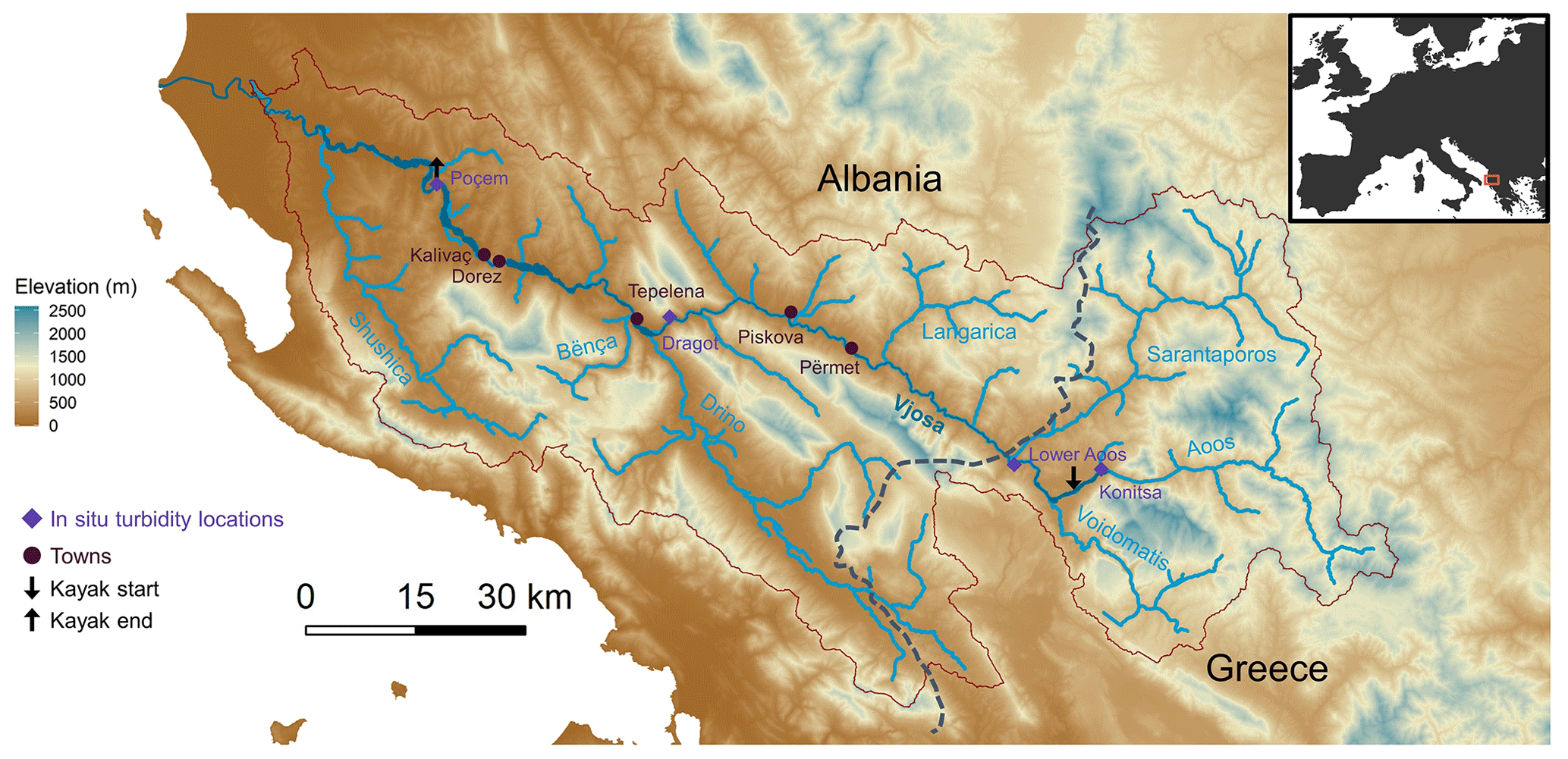
Figure 1 The Vjosa River catchment. The river originates in the mountains of Greece and travels northwest through Albania before reaching the Adriatic sea. The Vjosa main stem (dark blue) and its five main tributaries (light blue) are marked. Some main towns are marked in dark red circles, the in situ turbidity gauging stations are in purple diamonds, and the start and end of the kayak trips are marked with arrows. The catchment area is delineated by the red outline.

The Vjosa (known as Aoos in Greece) consists of five major tributaries: Voidomatis, Sarantaporos, Drino, Bënça, and Shushica. In this study, we focus on the main stem of the river from Konitsa to the outlet (Fig. 1).

The Vjosa River is poorly gauged. Daily streamflow is available only at Dorez (Fig. 1) for the period 1958–1989 (Schiemer et al., 2018b; Pessenlehner et al., 2022). Past bedload and suspended load measurements were only available from irregular and short field campaigns in 2018 by Pessenlehner et al. (2022) at Poçem (Fig. 1). For this research, we installed four turbidity sensors on the main stem (orange diamonds in Fig. 1). The sensors, Aqua TROLL 600 by In-Situ, measured water temperature, turbidity, pressure, dissolved oxygen concentration, and dissolved oxygen saturation. The sensors took measurements every 15 min for 2 years from May 2019 to July 2021. Some of the sensors were lost throughout the study and did not record for this entire time period (Poçem and Konitsa sensors stopped recording in October 2019 and January 2021, respectively). Suspended sediment sampling was complemented by two kayak surveys in spring 2019 and fall 2020. These were 4 d trips during which a continuous turbidity profile was measured at 1 min resolution with the same sensor Aqua TROLL 600 attached to the bottom of a kayak. We call these Lagrangian river profiles as the paddler was travelling downriver at speeds similar to or higher than the flow velocity. To fit the SSC–turbidity relationships we also periodically collected bottle samples, which were filtered to obtain SSC.

Spatial data for the catchment were obtained from E-OBS (daily precipitation) and CORINE (landcover). The digital elevation model (DEM) was obtained from Copernicus Digital Elevation Model (COP, 2019) and has a spatial resolution of 24 × 24 m. The DEM was used to derive flow accumulation along the river network and to compute river reach gradients. Daily precipitation data were averaged at subcatchment scales and summed over extended periods prior to the dates of satellite images as a proxy for runoff generation and streamflow.

2.2 Estimating turbidity from Sentinel-2 images

In order to estimate turbidity from the satellite images, the images first needed to be processed (atmospheric correction, cloud removal, etc.) and clipped to the studied river section. A regression model was fitted using the data from the in situ turbidity sensors and from the satellite pixels surrounding these sensors. This regression equation was then used to estimate turbidity for the entire main stem of the river for all available satellite images. The workflow of the procedure is shown in Fig. 2, and the following sections explain the procedure in more detail.

2.2.1 Satellite images

Sentinel-2 (S2) satellite images over the catchment were collected for this study for the sensing period May 2019–July 2021 from the Copernicus Open Access Hub. Sentinel-2 products were chosen because they provide 10 m resolution images in the red (665 nm), green (560 nm), blue (490 nm), and near-infrared (NIR, 842 nm) bands. As the average active channel width of the Vjosa River ranges between 30 and more than 600 m depending on river reach (Hauer et al., 2021), the S2 images are sufficient to resolve the flow width in most of the river reaches. Sentinel-2 also provides six additional 20 m resolution bands, one of which is the short-wave infrared band (1610 nm), which we used to identify deepwater sections. Sentinel-2 records the radiance reflected from the top of the Earth's atmosphere across different parts of the electromagnetic spectrum; these products are called Level-1C (L1C). The ESA also provides Level-2A products, which are the bottom-of-atmosphere (BOA) reflectance images derived from atmospherically correcting the associated L1C products (ESA, 2022). However, in this study we use the L1C products and atmospherically correct the images ourselves using an algorithm that was specifically designed to process small, turbid, inland waterbodies (Vanhellemont and Ruddick, 2016). To cover the entire catchment during the study period, two S2 L1C images (tiles T34TCK and T34TDK) were downloaded every 5 d and stitched together. This gives us a total dataset of 106 images in the study period (55 images from May 2019–July 2020, 51 images from August 2020–July 2021).

2.2.2 Image processing methodology

The methodology used to process the S2 images is summarized in the flowchart in Fig. 2. Downloaded L1C products (step 1., Fig. 2) were corrected (step 2., Fig. 2) to eliminate atmospheric noise, negative reflectance values, and sunglint using the Python-based processor ACOLITE (Vanhellemont and Ruddick, 2016), and the remote sensing reflectance (R_rs) in different spectral bands (e.g., 665, 560, 490, 842, 1610, and 2190 nm) was extracted. The resulting atmospherically corrected images were then clipped (step 3., Fig. 2) to the active floodplain boundary to minimize the amount of data that needed to be processed. A manually created shapefile was used to outline the active floodplain boundary, similar to what would be mapped in a hydrogeomorphological context (e.g., Hauer et al., 2021). The remote sensing signal from a water surface contains two components, sub-surface reflectance from particles suspended in the water and bottom reflectance from the riverbed. The sub-surface reflectance contains information on water clarity and is of interest to us, while the bottom reflectance is a noise component. Deepwater sections are less likely to have bottom reflections and can be distinguished by their low reflectance in the short-wave infrared band of wavelength 1610 nm (Ji et al., 2009). For this reason, we first resampled the 1610 nm image (20 ×20 m resolution) into a 10 ×10 m grid and then extracted the deepwater pixels by using an upper cutoff value of 0.045 sr⁻¹ (step 4., Fig. 2). This cutoff value was chosen for $R_{{\mathrm{rs}}_{\mathrm{1610}\mathrm{nm}}}$ (pixel values are from 0 to 1) through a visual inspection of the river. We began by applying different cutoff values to try to detect known deepwater locations along the river. The cutoff value that was able to objectively detect the known deepwater locations along the river was selected. The contingency table created for this cutoff method had a sufficiently low false negative rate of 7 %. In using the cutoff on $R_{{\mathrm{rs}}_{\mathrm{1610}\mathrm{nm}}}$ we not only extract the deepwater pixels within the active floodplain but also remove all other pixels (vegetation, dry bank surfaces, other water that is not deep, etc.). Our procedure also included the removal of pixels that are affected by clouds and cloud shadows (step 5., Fig. 2), with a MATLAB-based masking algorithm called function of mask (Fmask; Qiu et al., 2019). We used the default parameters in Fmask for Sentinel-2 images; therefore, a cloud probability threshold of 20 % was used in the processing. Fmask then detects the clouds (and cloud shadows) present in the image and removes only these affected pixels in the image. We would also like to point out that our methodology for processing the satellite images does not consider adjacency effects. The dark spectrum fitting (Vanhellemont, 2022) algorithm used in this study is meant to avoid some of the issues associated with atmospheric correction over water in the presence of adjacency effects (Vanhellemont and Ruddick, 2018; Vanhellemont, 2019). Past studies have found that adjacency effects may not occur over all inland waterbodies (Pahlevan et al., 2018) but they are important and should be investigated for narrow (and wide) rivers. However, investigating the effect of land adjacency would go beyond the scope of this work.

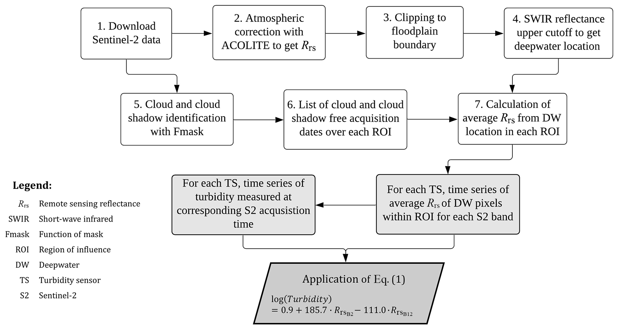
Figure 2 Flowchart summarizing the satellite image processing methodology and how to build the regression from the images. Steps (1)–(6) describe the image processing. Pixels in a 200 m diameter region of interest (ROI) around the sensors are averaged for each R_rs band (step 7). These average R_rs bands in deepwater (DW) pixels at the time of corresponding in situ measurements are used to build the regression using Eq. (1).

2.2.3 Building a regression model

A regression model was built by relating the in situ turbidity measurements at the four ground stations to the pixels in the immediate vicinity of the sensors. To obtain the representative reflectance coming from the water column surrounding the sensors, and not relying on a single pixel above the sensor, a circular buffer was selected around each sensor to mark its region of influence (ROI). The extent of the ROI was fixed at 200 m after comparing the mean reflectance of deepwater, cloudless pixels within ROIs of different radii (500, 200, 100, and 10 m). After removing the clouds, cloud-shadows, and non-deepwater pixels within each ROI, the average R_rs for each spectral band was calculated (step 7., Fig. 2) for every satellite image. This resulted in on average 280 pixels (28 000 m²) in each ROI for each acquisition day. In addition, at each sensor location, we extracted the closest in situ turbidity measurements corresponding to the satellite acquisition times (where the maximum time offset between the satellite image and in situ turbidity acquisition times is 15 min). This resulted in a dataset containing the average R_rs of the 11 S2 bands and the in situ turbidity data for each sensor location (ROI) over 2 years. This gave us 236 data points (13 at Poçem, 56 at Dragot, 75 at lower Aoos, and 92 at Konitsa).

A multiple linear regression analysis using ordinary-least-squares (OLS) was performed on the above dataset using the in situ turbidity data (response variable in the range of 0–2800 NTU) and the average R_rs of the 11 S2 bands as separate potential predictor variables, with the goal to determine the regression line whose sum of squared residuals errors is minimum. We did this because we do not want to prescribe a priori bands for the regression model but rather let the data dictate the best fit. Histograms of average R_rs and turbidity data were checked to identify variables that require transformations which would result in better fitted regression models. A logarithmic transformation was applied to in situ turbidity, converting its probability distribution from a right-skewed to a normal distribution and making log(turbidity) the new response variable. To avoid multicollinearity between the predictor variables which would lead to poor model fit, checks based on pairwise correlation coefficients and variance inflation factors (VIFs) were performed to choose only one among each set of collinear predictors (the correlation values between log(turbidity) and the different bands are shown in Table S1 in the Supplement). After this step, regression models were fitted to different combinations of the chosen predictor variables (the 11 S2 bands), including different band ratios and their combinations, and the corresponding Bayesian information criterion (BIC) was compared. This way, only the average R_rs S2 bands (predictors) that have the highest, and independent, predictive power for in situ turbidity (in NTU) were chosen, as the BIC favours smaller, less complex models.

3 Results and discussion

3.1 Regression model and uncertainty

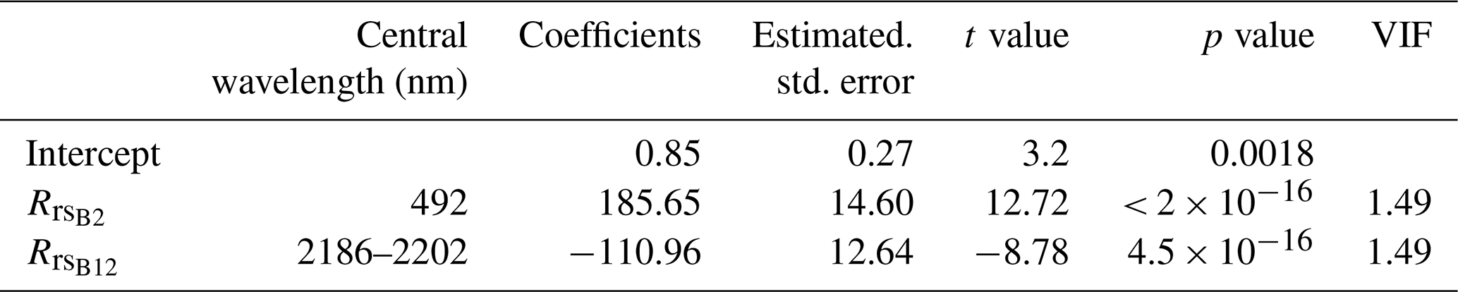
The best performing multiple linear regression model for log(turbidity) in NTU following the workflow in Fig. 2 described above was

$$\begin{array}{}\text{(1)}& \log \left(\mathrm{turbidity}\right)=\mathrm{0.9}+\mathrm{185.7}\cdot R_{{\mathrm{rs}}_{\mathrm{B}\mathrm{2}}}-\mathrm{111.0}\cdot R_{{\mathrm{rs}}_{\mathrm{B}\mathrm{12}}}\end{array}$$

The model was built with 226 data points and the residual standard error of the model is 1.613 log(NTU) or 5 NTU. Using the NTU–SSC rating curve, which we developed from observations (discussed later in Sect. 3.4), this gives us an error of 23.8 mg L⁻¹. The adjusted R² of the model in Eq. (1), which explains the portion of the variance in turbidity by the two predictors, is R²=0.42 (p value < 2 × 10⁻¹⁶). The model statistics are shown in Table 1 and the 3D regression plot is found in Fig. S2. The p values indicate a statistically significant relationship between the predictor(s) and the response variable. The variance inflation factors (VIFs) are < 5, meaning there is no multicollinearity problem present between the chosen predictors.

Table 1 Statistics for chosen regression model.

It is very difficult to compare our established relationship with those given in literature. First, not many satellite studies have been conducted on rivers at this scale (due to spatial resolution). Second, because the relationships are purely empirical and dependent on sensor quality, frequency bands used, image processing, number of data points contained in the regression, sediment properties, flow regime, etc., there is little reason to expect any generality in the form of the predictor–response relations. Nevertheless, here we compare our results with some selected studies.

Onderka and Pekárová (2008) obtained a linear equation between the suspended particulate matter (SPM) and the calibrated radiance of the Landsat NIR band using a single-day image of the Danube. The equation had a standard error of 2.92 mg L⁻¹ (R²=0.95). However, their regression was built using 3 samples (0–60 mg L⁻¹) and validated using 12 samples (0–20 mg L⁻¹) only. Most of these samples came from a small impoundment area (∼ 16 km long). Bernardo et al. (2017) generated a quadratic equation relating total sediment matter (TSM) to the OLI5 band (narrow NIR) of the Landsat-8 satellite (p value < 0.01 and R²=0.67, satellite revisit time of 8 d). Their model was built on the Barra Bonita Hydroelectric Reservoir (series of reservoirs along the Tiete and Piracicaba rivers) using 23 samples over 2 sampling days. They were also able to achieve a low RMSE of 3.59 mg L⁻¹. Iacobolli et al. (2019) built an SSC empirical exponential equation using the 665 nm (red) S2 spectral band (R²=0.05). This was done with 35 samples from the estuary of the Aterno-Pescara river in Abruzzo and gave an RMSE of 4.74 mg L⁻¹. The low errors in predicted SSC in all three studies above can be attributed to the small sampling interval, which covers only a narrow range of possible sediment concentrations, and the small area considered in the regression fits.

Doxaran et al. (2002) built a third-order polynomial using the reflectance ratio between NIR (850 nm) and green visible (550 nm) wavelengths of the SPOT satellite. They were able to estimate a TSM concentration of between 15 and 250 mg L⁻¹ (R²=0.64). The polynomial was built with 34 samples (13–985 mg L⁻¹) taken in July 2000, September 2000, July 2001, August 2001, and September 2001 at four locations (15–22 km apart). Wass et al. (1997) used the Natural Environment Research Council (NERC) Compact Airborne Spectral Imager (CASI) to extract turbidity and SSC from the Humber Estuary. Samples were collected from the bed of the estuary and calibrated to a spectrometer in a mixing tank for the range 0–2000 mg L⁻¹. A linear relationship (R²=0.95) was established between SSC and the 755.5–780.8 nm band (vegetation red-edge band). Unfortunately, neither of these works report the error of the regressions.

Sahoo et al. (2022) could achieve RMSE of 42.8–49.85 mg L⁻¹ and R² of 0.65–0.77 on three different river sections of the Hooghly River using Aqua MODIS red band images. Finally, Wang et al. (2021) collected 62 SSC samples on the Yangtze River and, using partial least squares, built a power equation using the ratio of the narrow NIR to the green band (B8a / B3, for both S2 and Landsat 8, R²=0.78). They were able to obtain an RMSE of 24.1 mg L⁻¹, which is close to what we were able to obtain in our regression.

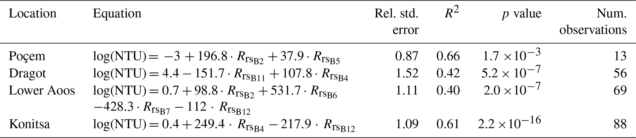
One commonality in the studies above is the use of red or NIR in the empirical relationships. Therefore, our use of the IR band should not be surprising. Several of the above-mentioned studies conducted regression analysis on shorter river sections, which will lead to a smaller standard error because local variability due to flow depth, bed morphology, land use, geology, etc. is reduced. In order to create longitudinal turbidity profiles of the entire Vjosa main stem (272 km), our regression in Eq. (1) was built on all four turbidity gauging stations at the same time, so that it also captures inter-site differences at the larger river basin scale. When, instead, regression models were built for individual gauging stations with a 200 m ROI buffer, we obtained lower standard errors (Table 2). All of the relative standard errors for the individual regressions (relative standard errors between 0.87 and 1.52) are slightly lower than the error from the regression for all stations together (relative standard error of 1.61). Additionally, the individual stations have R² larger than or equal to the original R²=0.42 but their models chose entirely different bands than the original bands in Eq. (1); however, all of the selected bands in the new equations are either red or IR, as expected. However, predicting turbidity of the main stem using any one of these single-station regressions could lead to large prediction errors in river reaches with completely different geology, river morphology, and sediment sources/sinks. Additionally, the original Eq. (1) does not perform dramatically worse than the individual station models.

Table 2 Model statistics for individual buffer stations at four locations along the main stem.

3.2 River turbidity profiles: validation and seasonality

The first aim of this paper was to extract the river turbidity profiles from the satellite imagery and investigate the spatial and seasonal signals present in the turbidity profiles. To this end, the regression equation from Eq. (1) was applied to every processed (cloud and cloud-shadow free, deepwater, atmospherically corrected) Vjosa pixel in 106 images over 2 years (55 images from May 2019–July 2020, 51 images from August 2020–July 2021). Applying the regression to all of the river pixels resulted in 106 turbidity maps, one of which is shown in Fig. 3a (from 23 October 2020). When all 106 images are averaged in time and binned into 100 m river segments in space to reduce pixel-to-pixel variability, we see an interesting signal of spatial variability in mean NTU along the Vjosa main stem (Fig. 3b). Mean NTU over the 2-year period varies from near 0 in the upstream sections to between 200 and 300 NTU in the lower sections. The maximum predicted turbidity was 9856 NTU. Some of the spatial variability is connected to inputs from tributaries (e.g., Drino and Bënça), but there is also systematic variability within river sections that do not have large tributary inputs (e.g., between 20 and 100 km upstream the outlet in Fig. 3b).

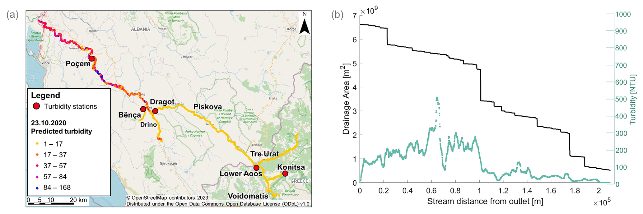
Figure 3 Turbidity data extracted from Sentinel-2 imagery for the entire Vjosa catchment using © OpenStreetMap contributors 2023. Distributed under the Open Data Commons Open Database License (ODbL) v1.0. (a) Processed turbidity map for 23 October 2020. (b) Two-year-average longitudinal turbidity profile (green) and catchment area from the DEM (black), both plotted against the stream distance from the outlet.

A proper validation of the predicted river turbidity profiles from satellite imagery is not possible, as we do not have spatially distributed turbidity sensors along the river system. Instead, here we conducted a qualitative comparison with the kayak-derived river turbidity profiles. Using these types of Lagrangian measurements in rivers is not uncommon (Hensley et al., 2014; Baker et al., 2014; Kraus et al., 2017; Postacchini et al., 2015). Therefore, we collected two turbidity profiles from a kayak; these are shown in Fig. 4: one in spring 2019 (Fig. 4a) and one in fall 2020 (Fig. 4b). Since the river is 272 km long, the measurements were taken over 4 d kayak trips during a period with no rainfall in the catchment. The sensor used was the same Aqua TROLL used at the ground stations, with a 1 min sampling resolution during the descent. Discharge in these plots was estimated using a log–log scaling relationship between catchment area and discharge. Discharge was measured empirically at selected sampling sites using an electromagnetic flowmeter (Ott MF Pro, Ott Hydromet, Kempten, Germany) at a minimum of 15 sites spread evenly across a river transect or by means of an acoustic Doppler profiler (SonTek River Surveyor) towed across the river and delivering a spatially continuous velocity field. These measurements were then used as calibration points in a Bayesian regression with priors taken from published scaling relationships (Burgers et al., 2014). Two discharge measurement campaigns were conducted: one in spring 2019 and one in fall 2019 (the latter was used to plot Q⋅T in Fig. 4b as a proxy for fine sediment load).

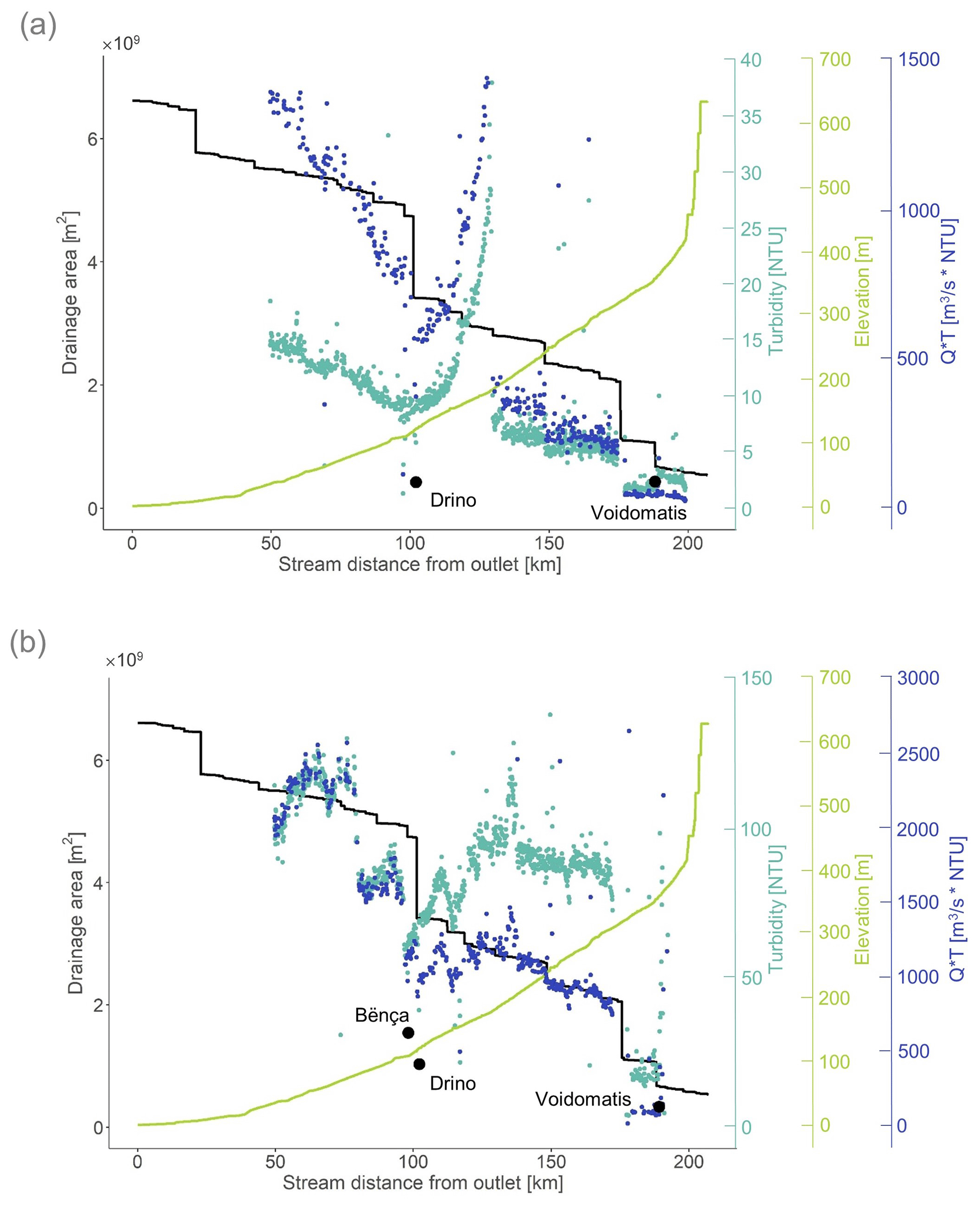
Figure 4 Longitudinal profiles from the kayak trips plotted along the distance from the outlet in (a) spring 2019 and (b) fall 2020. Teal points are turbidity measured by the Aqua TROLL 600. Blue points represent a proxy for sediment load (discharge, Q, multiplied by turbidity, T). The green line is the elevation of the riverbed and the black line is the catchment area, both extracted from the DEM. Three larger black points mark the turbidity of the tributaries: Bënça, Drino, and Voidomatis.

Although the kayak-derived measurements cannot be directly compared with individual satellite images as the former are Lagrangian estimates over a 4 d sampling window, and the latter are snapshots in time which does not necessarily overlap with this window, we still can use these data to provide a qualitative check of the satellite data. Figure 4 reveals some consistent patterns in sediment inputs and fluxes. In both spring and fall, as the Sarantaporos joins the Aoos (at 175 km from the outlet) both the turbidity and the Q⋅T increase. This increase is also evident in the satellite data in Fig. 3b with similar NTU values. There is also a peak at around 130 km near Piskova (see Fig. 1 for location) in 2019 that quickly decays. This appears to be a sediment wave that was generated in one of the tributaries and which passes downriver. Both the turbidity and Q⋅T near Poçem (see Fig. 1 for location) is higher than in the headwaters and reaches about 15 NTU in 2019 and 120 NTU in 2020 in the kayak-derived data, while on the average the satellite images predict about 200 NTU for this location. As the kayak measurements were conducted during dry weather and low flows while the satellite data cover an entire 2-year period with seasonality present, this difference is expected.

We now use the 106 satellite images to compute mean seasonal turbidity along the Vjosa main stem. Figure 5 shows a seasonal signal across 2 years of measurements, from May 2019–July 2021. It is evident that mean turbidity in the Vjosa is higher in winter than the other seasons, especially summer. Interestingly, in Piskova (130 km from outlet), there is a peak in turbidity that is seen in the winter signal and not in the other seasons. This winter peak is evident also in the 2-year average in Fig. 3b and in the kayak-derived observations in Fig. 4. There are other recurring patterns in the seasonal signals and in the river profiles, for example, the jump in turbidity due to the Drino tributary at 100 km and the dip in the braided section (75 km). By inspecting individual images we conclude that these consistent changes in turbidity are independent of seasonality and likely have to do with persistent sediment sources and sinks in these river reaches.

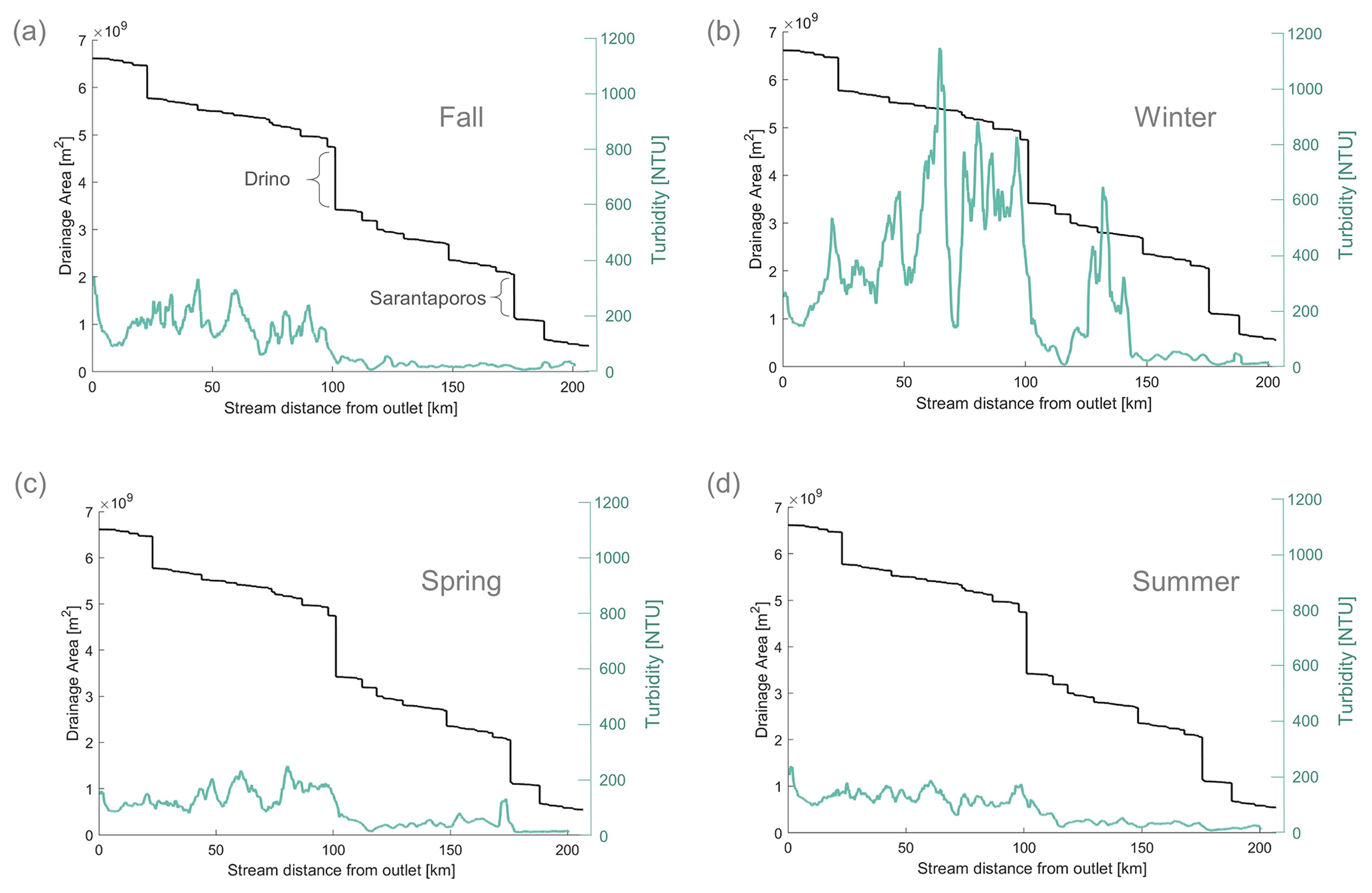
Figure 5 Seasonal longitudinal turbidity profiles (blue-green) and catchment area from the DEM (black), both plotted against the stream distance from the outlet. (a) Fall is the average of all longitudinal profiles extracted from satellite images from September to November in both 2019 and 2020 (the two largest tributaries, Sarantaporos and Drino, are marked), (b) winter is from December 2019 to February 2020 and then again from December 2020 to February 2021, (c) spring is from March to May in both 2020 and 2021 and with one additional image from May 2019, (d) summer is from June to August in 2019 and 2020, and June to July in 2021.

3.3 Sources and sinks of sediment along river profiles

The second aim of this paper was to identify possible fine sediment sources and sinks in the Vjosa catchment from the longitudinal river turbidity profiles due to tributaries and within individual river reaches, and search for their possible activation by rainfall. To achieve this aim, we computed changes in NTU upstream and downstream of every tributary dNTU_trib and upstream and downstream of every river segment dNTU_rea (Fig. 6).

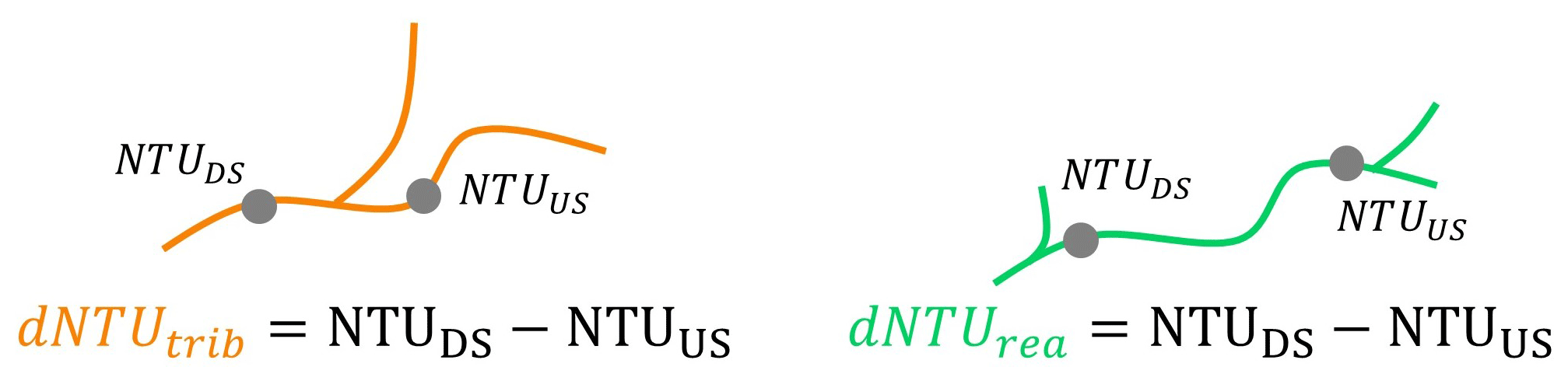
Figure 6 Differences in turbidity (dNTU) calculated as the upstream turbidity subtracted from the downstream turbidity. The locations of upstream and downstream turbidity are shown in the two panels: left for tributaries and right for river reaches between two tributaries.

Boxplots of dNTU from all 106 satellite images are shown in Fig. 7 where the x axis gives the relative location of each tributary or centre of reach (not to scale). If a tributary brings disproportionately more sediment or if sediment is mobilized within the reach (e.g., from the bed or banks), then dNTU > 0 and there is a sediment source. Conversely, if dNTU < 0, then water added by the tributary brings less sediment or there is deposition of sediment within the reach and we have a sediment sink. The asterisks in Fig. 7 represent the sources and sinks with a statistically significant change in dNTU. The kayak-derived measurements in 2019 and 2020 are also shown as markers in the boxplots. Most of the kayak points fall within the whiskers of the dNTU boxplots, confirming that the measurements taken during these low-flow conditions lie within the natural variability in turbidity at those locations. The kayak points all fall within the boxplot whiskers except for the most upstream reaches/tributaries (at $L/Lx=\mathrm{0.81},\mathrm{0.88},\mathrm{0.91},$ and 0.94). There we theorize that the river is too narrow in the upstream section to extract proper reflectance data. Also, the river is much more clear upstream so the measurements from satellite images may fail.

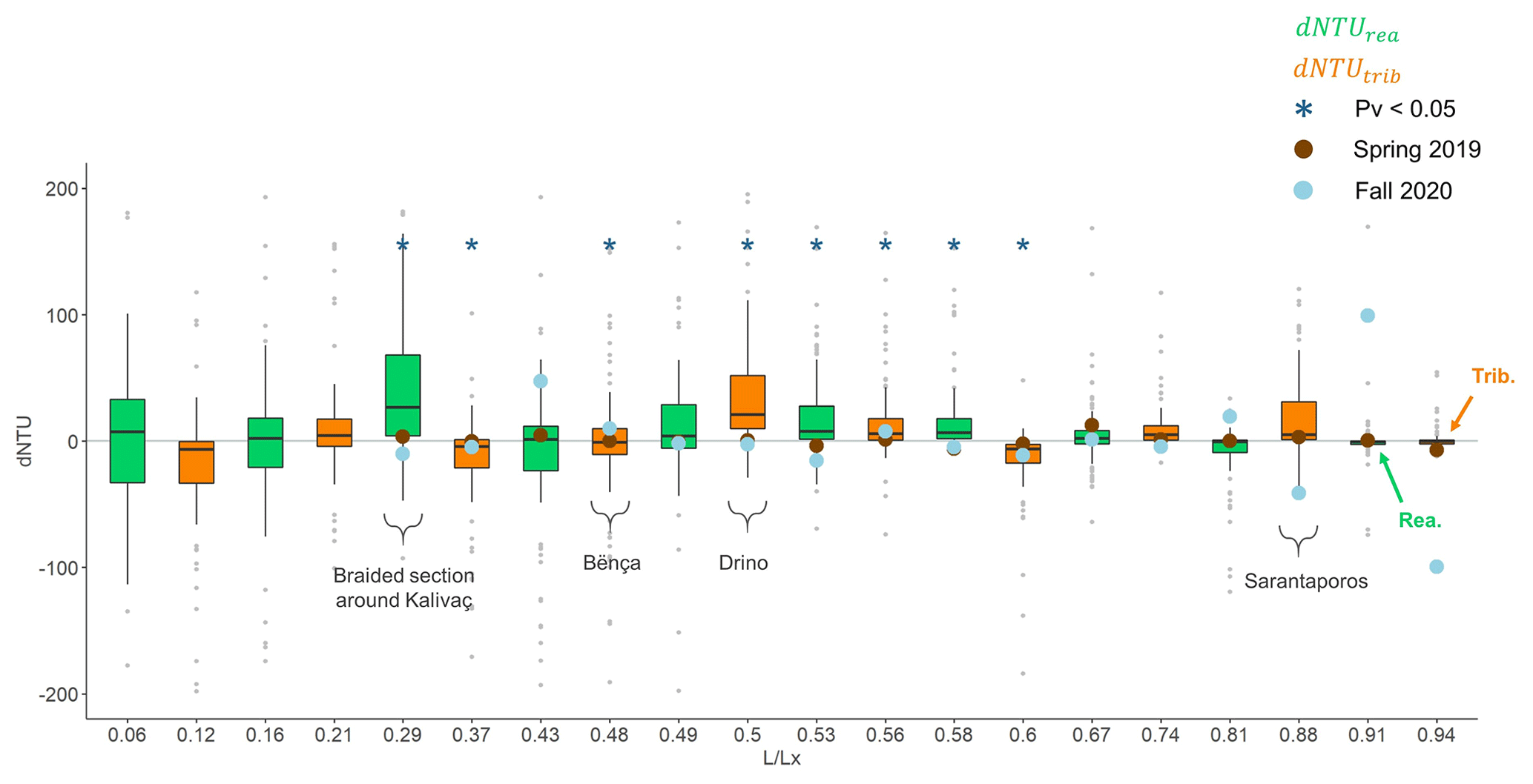
Figure 7 Boxplots of differences in satellite-derived turbidity (dNTU) for tributaries (orange) and reaches (green) plotted against the relative stream distance from the outlet ($Lx/L$). The boxplots were built using the 106 turbidity profiles over 2 years. The black line in the boxplot represents the median, the boxes extend to ±1 standard deviation, the whiskers extend to ±1.5 ⋅ IQR, and the light grey points are the outliers. Locations with a p value < 0.05 are marked with a blue asterisk. The kayak points from spring 2019 and fall 2020 are marked as the brown and light blue circles, respectively. Some major tributaries and reaches are labelled.

The statistically significant fine sediment sources are found at $Lx/L=\mathrm{0.29},\mathrm{0.53},\mathrm{0.58}$ (reaches) and 0.5, 0.56 (tributaries). These river reaches and tributaries are surrounded by agricultural land and located in predominantly Flysch and clastic sediment geologies. All three of these factors could contribute as sediment sources to the increase in SSC. The two reaches at $Lx/L=\mathrm{0.53}$ and 0.58 are located within limestone canyons with springs; therefore, we expect a decrease in SSC from the spring water dilution. However, we find that the SSC increases as we move downstream. One possible reason could be that river water is infiltrating into the bed in these limestone reaches, leaving a higher sediment concentration in the main stem. This would have to be confirmed with flow measurements. The reach at $Lx/L=\mathrm{0.29}$ has the largest median and variability in all of the statistically significant sources. This reach contains a large braided section which can act as a source of fine sediment from the riverbed during high discharge conditions and also as a sink during low discharge conditions. This reach however could also be a source due to since-abandoned dam construction activities in Kalivaç, which might have been producing larger quantities of fine material in recent years.

The statistically significant fine sediment sinks in the Vjosa are fewer than sources and are located at $Lx/L=$ 0.37 and 0.6 (tributaries). The estimated rates of change dNTU here are likely caused by systematically lower sediment concentrations coming from these tributaries than already present in the main river. Although we could not identify relevant differences in catchment geology, vegetation cover, or steepness in these catchments, it is conceivable that they have low sediment production rates. However, it is also notable that the changes in NTU downstream of these tributaries are very small, often close to the standard error of the regression model in Eq. (1), and furthermore, at $Lx/L=\mathrm{0.37}$ the downstream section is constricted in a canyon with poorer satellite visibility. All of these factors result in the predictions here being highly uncertain.

We hypothesize that the tributary and reach changes in NTU should be related to the strength of activation of sediment sources by rainfall and runoff. We test this hypothesis by dividing all tributary and reach dNTU into wet and dry days. Of our 106 available days/satellite images, we could obtain rainfall data for 101 d (up until the end of June 2021). We define dry days as days where there is less than 0.01 mm of cumulative rain over the last 6 d in the entire catchment and wet days are all other days (67 wet days and 34 dry days). On dry days, mean dNTU =7.5 for river reaches and dNTU =2.5 for tributaries, suggesting that there is very little sediment activation and sediment concentration is almost constant, while on wet days, mean dNTU =4.4 for river reaches and dNTU =30.2 for tributaries, suggesting that tributaries indeed become sediment sources by rainfall-activated mobilization.

The empirical cumulative distributions of the dNTU rates in Fig. 8 show that rainfall affects both river reaches (Fig. 8a – green) and tributaries (Fig. 8b – orange) in the extremes. Interestingly, the dNTU of river reaches tends to deviate stronger from dNTU =0 in both the positive and negative directions (acting as both sources and sinks) with the presence of rainfall. However, tributaries tend to act more as sources (dNTU >0) with the presence of rainfall. Performing a two-sample Kolmogorov–Smirnov test on the wet and dry day distributions for both the tributaries and reaches, we find that the two distributions (dry and wet) are statistically significantly different (for tributaries: D_KS=0.15 and p value $=\mathrm{1.58}\times {\mathrm{10}}^{-\mathrm{4}}$; for reaches: D_KS = 0.12 and p value $=\mathrm{5.42}\times {\mathrm{10}}^{-\mathrm{3}}$). The p value is reported for a significance level of 5 %.

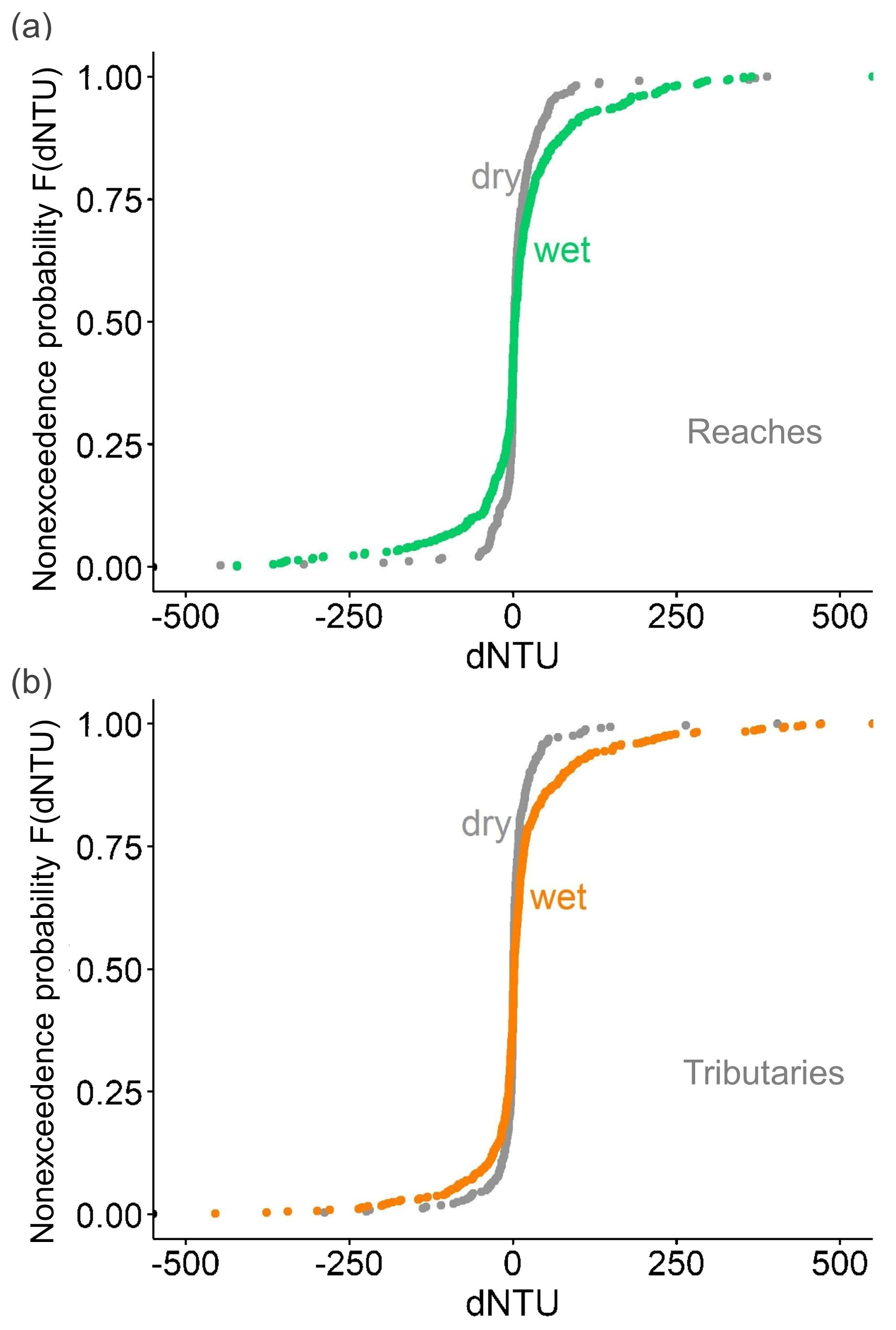
Figure 8 Empirical cumulative distributions for reaches (a) and tributaries (b) on dry and wet days.

3.4 Sediment load at Dorez

Finally, we conducted a plausibility check to see if the estimates of SSC and sediment load at Dorez (the single gauged location on the Vjosa River) from our remote sensing-derived turbidity estimates agree with SSC estimates of past studies. Using the satellite river turbidity profiles, we could estimate the annual sediment yield at Dorez, 70.5 km from the outlet (see location in Fig. 1). First, we computed the mean seasonal turbidity at the Dorez location in the longitudinal profile from the 2 years of satellite data in Fig. 9a (e.g., SON boxplot is September, October, and November turbidity values in the years 2019–2020). The boxplots were built using all the turbidity pixels around Dorez (70.46–70.58 km from the outlet). Second, the mean turbidity values were converted to SSC using the rating curve in Fig. 9b, where a power fit was found to best represent the NTU–SSC relationship (Holliday et al., 2003). The SSC data for this fit were obtained by taking water-sediment (gravimetric) samples on the main stem during our various campaigns from 2019 to 2021. Subsequently, after each campaign the gravimetric samples were filtered using Whatman GF/F filters, the filters were weighed to obtain the sediment mass (mg), and the volume of filtered water was measured and combined with the volume of the filtered sediment to obtain the total volume of the sample (L): this gave us the SSC in mg L⁻¹. These gravimetric samples were taken at Poçem, Dragot, Lower Aoos, and Konitsa (see Fig. 1). Similarly to the catchment-wide turbidity–R_rs relationship of Eq. (1) (as opposed to different relationships applied to different reaches, as explained in Sect. 3.1), we wanted to create a catchment-wide turbidity–SSC relationship. This relationship was also necessary since we have neither SSC samples nor turbidity measurements in the Dorez reach. Additionally, although this relationship introduces uncertainty when estimating SSC in the Dorez reach, it can be applied to any section of the river. Using the turbidity–SSC relationship in Fig. 9b, the 2-year seasonal average SSCs were found to be as follows: winter – 10.4 g L⁻¹, spring – 5.1 g L⁻¹, summer – 8.5 g L⁻¹, and fall – 14.9 g L⁻¹. Third, the daily discharge (m³ s⁻¹) at Dorez from 1958 to 1989 (Pessenlehner et al., 2022) was used to compute the mean seasonal discharge in 2-year periods, which corresponds to our measurement duration period. This daily discharge data from 1958 to 1989 was used because there are no alternative long-term discharge data available for the catchment. Two-year periods were averaged so that we capture possible natural variability at biannual timescales in the discharge record. The 2-year seasonal discharges were then multiplied by the mean seasonal SSC to get the seasonal sediment load for 2 years and cumulated to get total annual loads. This approach gives us biannual estimates of fine sediment loads which have the same seasonal mean concentrations as our estimates but different annual discharges. The results in Fig. 9c show that the resulting mean annual sediment yield in Dorez has a decreasing tendency due to lower discharges in time. Our best estimate of the mean annual sediment load at Dorez, assuming that sediment concentrations follow our estimates, is $\sim \mathrm{2.5}\pm \mathrm{0.6}$ Mt yr⁻¹, which is in agreement with 1.4–2.5 Mt yr⁻¹ reported by Pessenlehner et al. (2022) at this location.

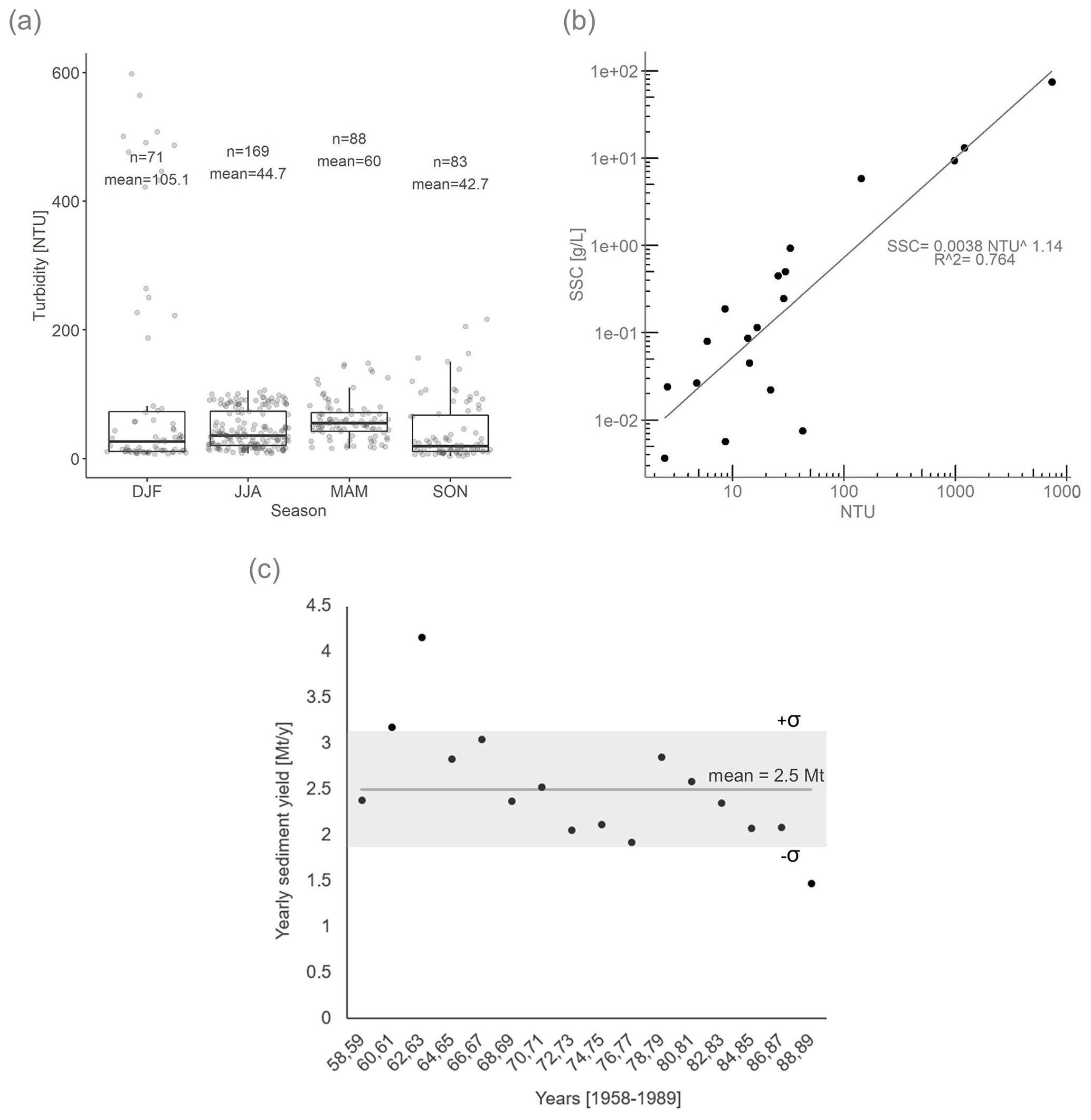
Figure 9 Sediment yield calculation. (a) Boxplots of turbidity at Dorez across 2 years grouped by season. The horizontal line in the boxplot is the median, the boxes extend to ±1 standard deviation, the whiskers extend to ±1.5 ⋅ IQR, and the points are the outliers. Above each boxplot is the number of observations and the mean for each season. There are more observations than the number of images (106 images, Sect. 3.2) because we took all of the pixels around Dorez (between 70.46 and 70.58 km from the outlet, mean of ∼ 5 pixels). (b) Power model fit between turbidity (NTU) and SSC (g L⁻¹) for seston samples we collected throughout our field campaigns. (c) Yearly sediment yield for 1958–1989, calculated using the seasonal turbidity averages over 2 years and discharge data from 1958 to 1989; the mean is marked with the grey line and ±σ is marked with the grey shading where σ=0.63 Mt.

A suspended sediment yield of $\sim \mathrm{2.5}\pm \mathrm{0.6}$ Mt yr⁻¹ is remarkable for such a small catchment. This amounts to an erosion rate of 373 t yr ⁻¹ km⁻² (for a catchment area of 6704 km²). In comparison to the Amazon, pre-dam Mississippi, St. Lawrence, and Yangtze rivers, which each produce 204, 124, 4, and 267 t yr ⁻¹ km⁻² of suspended load, respectively (Milliman and Farnsworth, 2013; Syvitski and Milliman, 2007). The sediment production by the Vjosa is similar to other small mountainous rivers nearby (Ofanto, Achelous, and Simeto rivers all have a catchment area less than 7000 km² and deliver 333, 611, and 238 t yr ⁻¹ km⁻², respectively; Milliman and Farnsworth, 2013). This puts the need for conservation of small mountainous rivers into perspective and enables us to understand Albania's push for the Vjosa National Park along the entire Vjosa River. Such a park would prevent any hydropower plants from being built, thus avoiding the obstruction of the necessary flow of sediment (Martini et al., 2022; Schiemer et al., 2018a, Chap. 1).

4 Conclusions

In this study, we have shown the potential and limitations of using high-resolution open-access satellite S2 images for estimating water turbidity in relatively narrow and morphologically complex rivers, with the purpose of detecting possible sediment sources and sinks and their activation by rainfall, as well as estimating sediment yield in mountainous catchments.

The first result presented here was the extraction of 106 longitudinal river turbidity profiles for the entire 270 km main stem of the Vjosa River in Albania for every available and cloud-free satellite image from May 2019 to July 2021 using a multivariate regression model fitted to four ground stations. The river profiles revealed variability in turbidity due to both tributary and within-reach inputs. The profiles also revealed a seasonal signal, with the highest mean turbidity in winter along the entire length of the river and visible local inputs by tributaries. Lagrangian river turbidity profiles were also measured along the entire main stem during two kayak trips and used as a qualitative validation of sediment concentration variability.

The second result presented here was that sediment sources and sinks could be identified and quantified from the river turbidity profiles, both for tributaries and within river reaches. The river basin and network acted as a sediment source most of the time; significant sediment sinks were rare but did exist. Sediment sources were mostly tributaries following basin-wide rainfall, but within-reach sources in river beds and banks were also possible. Finally, as a plausibility check we estimated the total fine sediment yield at Dorez at $\sim \mathrm{2.5}\pm \mathrm{0.6}$ Mt yr⁻¹, which is in line with previous studies and reveals the importance of the Vjosa River as a sediment source of the Adriatic, worthy of protection.

In this study, we have largely ignored the effects of land adjacency. It would be interesting to see a future study that investigates at which point (e.g., at which river width) does land adjacency not affect the pixels in the middle of the river. With this information, we could incorporate the effects of land adjacency and determine how to correct these effects. The methodology developed in this study may be applied to other river systems: this was our guiding principle. However, there are several steps that are site specific, e.g., downloading S2 images, developing shapefiles to delineate the floodplain boundary, and determining the deepwater threshold cutoff value (taken from visual inspection of known deep locations in the river), as well as the availability of at least one in situ sensor measuring turbidity to establish the turbidity–R_rs relationship. We see an opportunity of utilizing online tools (e.g., Google Earth Engine) to not only make the data processing faster (no need to store the S2 and processed ACOLITE images on a local drive) but also to create a transferable workflow for future studies.

Satellite images have been used for the quantification of turbidity in large waterbodies, wide rivers, lakes, and coastal zones. Here we show that such high-resolution data also have potential for suspended sediment quantification in smaller, narrower, and morphologically diverse mountain rivers, despite some loss in accuracy. The applications of such analyses are many, including identifying erosion hotspots, sediment source activation processes, various local point sources, and glacial channel networks in streams, large rivers, and river deltas. This work provides a proof of concept and workflow which lay the foundation for future studies to improve accuracy and reduce uncertainty in such analyses.