Topographic metrics for unveiling fault segmentation and tectono-geomorphic evolution with insights into the impact of inherited topography, Ulsan Fault Zone, South Korea

Quantifying today's topography can provide insights into landscape evolution and its controls, since present topography represents a cumulative expression of past and present surface processes. The Ulsan Fault Zone (UFZ) is an active fault zone on the southeastern Korean Peninsula that was reactivated as a reverse fault around 5 Ma. The UFZ strikes NNW–SSE and dips eastward. This study investigates the relative tectonic activity along the UFZ and the landscape evolution of the hanging-wall side of the UFZ, focusing on neotectonic perturbations using ¹⁰Be-derived catchment-averaged denudation rates and bedrock incision rates, topographic metrics, and a landscape evolution model. Five geological segments were identified along the fault, based on their relative tectonic activity and fault geometry. We simulated four cases of landscape evolution to investigate the geomorphic processes and accompanying topographic changes in the study area in response to fault movement. Model results reveal that the geomorphic processes and the patterns of topographic metrics (e.g., χ anomalies) depend on inherited topography (i.e., the topography that existed prior to reverse fault reactivation of the UFZ). On the basis of this important model finding and additional topographic metrics, we interpret the tectono-geomorphic history of the study area as follows: (1) the northern part of the UFZ has been in a transient state and is in topographic and geometric disequilibrium, so this segment underwent asymmetric uplift (westward tilting) prior to reverse faulting on the UFZ around 5 Ma, and (2) its southern part was negligibly influenced by the asymmetric uplift before reverse faulting. Our study demonstrates the utility of topographic metrics as reliable criteria for resolving fault segments. Together with landscape evolution modeling, topographic metrics provide powerful tools for examining the influence of inherited topography on present topography and for the elucidation of tectono-geomorphic histories.

1 Introduction

Research in the field of tectonic geomorphology involves identifying the signal of neotectonic activity from topography. The classic approach to such studies has traditionally relied on topographic metrics, with origins dating back to the 1900s (e.g., hypsometric integral, stream length–gradient index, and mountain-front sinuosity; Strahler, 1952; Hack, 1973; Bull, 1977; Cox, 1994; Keller and Pinter, 1996; Bull and McFadden, 2020). The normalized channel steepness index (k_sn; Flint, 1974; Wobus et al., 2006) and knickpoint analyses are also frequently applied to explore transient states of channels caused by tectonic activity (Whipple and Tucker, 1999; Duvall et al., 2004; Kirby and Whipple, 2012; Scherler et al., 2014; Marliyani et al., 2016), as channel incision is a direct response to tectonic uplift. The chi (χ) index was introduced to address limitations associated with slope–area analysis for calculating k_sn, which can be influenced by (1) noise and errors in topographic data and by (2) the resolution of the data themselves (Perron and Royden, 2013; Royden and Perron, 2013). Notably, the χ index facilitates a straightforward comparison of k_sn values across different channel reaches as the slope of the χ–elevation profile directly reflects the k_sn value (Perron and Royden, 2013). It has been applied to determine whether a landscape under specific conditions is in a steady state or transient state and to assess long-term drainage mobility (Willett et al., 2014; Forte and Whipple, 2018; Kim et al., 2020; Hu et al., 2021; Lee et al., 2021). As computational power has improved and as powerful modeling programs have become more widely available, it has become possible to simulate landscape evolution. We can test the site-specific parameters constrained by empirical data (e.g., coefficient of diffusivity, coefficient of fluvial erosion efficiency, and local uplift rate) and determine ranges of reasonable values through modeling (e.g., Tucker et al., 2001; Braun and Willett, 2013; Goren et al., 2014; Campforts et al., 2017; Hobley et al., 2017; Barnhart et al., 2020; Hutton et al., 2020). Modeling also facilitates the understanding of geomorphic processes and accompanying topographic changes in given tectonic and climatic settings by providing a visualization. These advances have allowed researchers to explain the state (equilibrium or disequilibrium) of present topography and to predict future landscape evolution within neotectonically active areas (Attal et al., 2011; Reitman et al., 2019; Zebari et al., 2019; Su et al., 2020; He et al., 2021; Hoskins et al., 2023).

Most of the studies mentioned above focus on using topographic analyses to identify spatial and temporal variations in lithological, tectonic, and climatic conditions. However, such studies do not generally account for the effects of inherited topography (i.e., topography prior to the neotectonic events of interest) on subsequent geomorphic processes, present topographic dynamics, and topographic metrics. We hypothesize that the influence of inherited topography can be non-negligible in our study area, where the fault slip rate is low, and the erosion rate is high, and topographic metrics would indicate it. Our hypothesis is based on the understanding that (1) the present topography is a cumulative result of past and present tectonic and climatic events, (2) the response time of geomorphic features (such as longitudinal stream profile, knickpoint migration, and divide migration) to the same tectonic events varies (Whipple et al., 2017), and (3) the timescale that each topographic metric represents is different and not yet fully understood (Forte and Whipple, 2018). Therefore, we propose that topographic metrics can reflect the cumulative influence of past and present geomorphic processes and their drivers and that drawing inferences from these indices without accounting for the influence of inherited topography can lead to misinterpretations of landscape evolution.

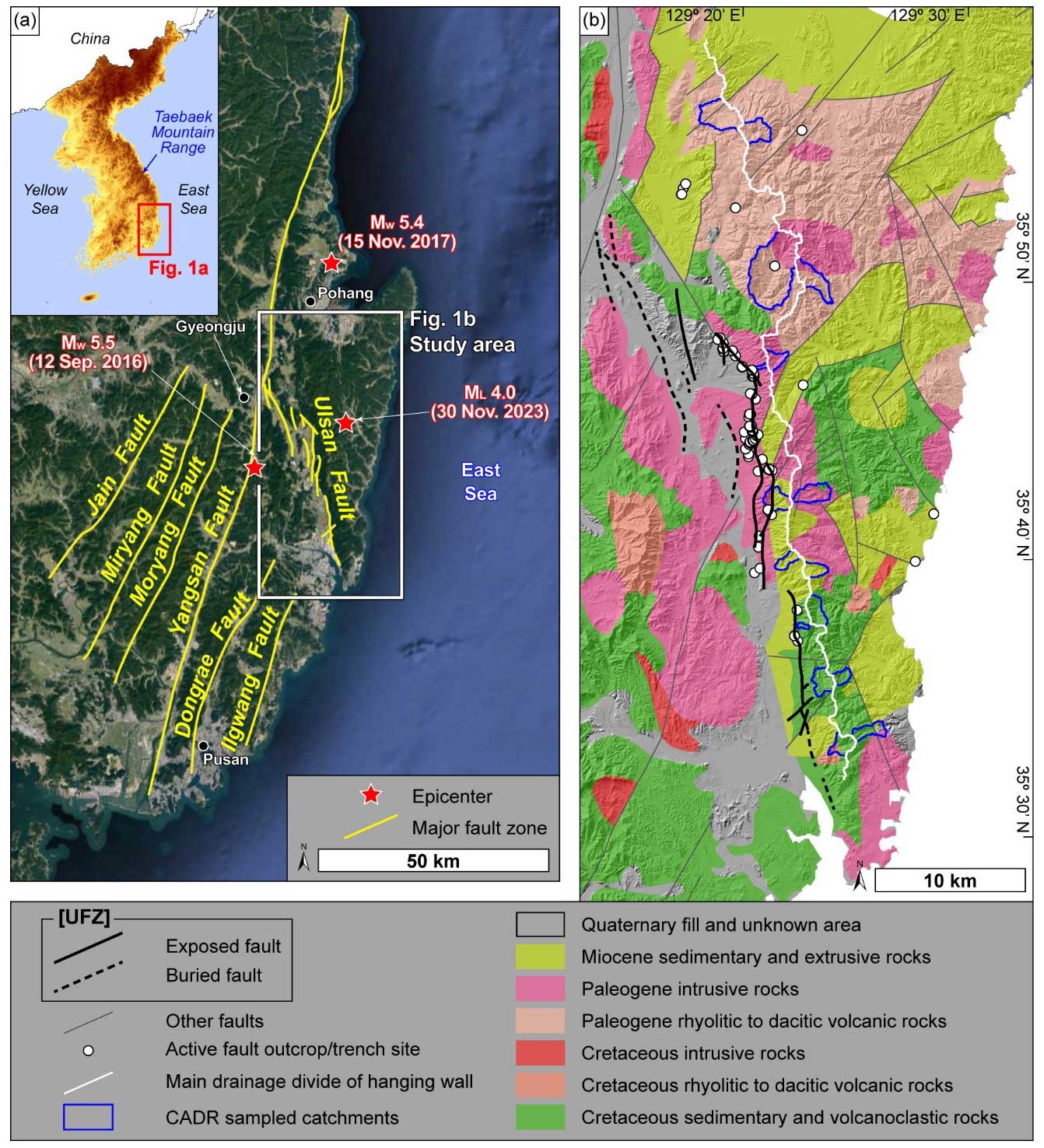
Figure 1 (a) Major fault zones on the southeastern Korean Peninsula (modified from M.-C. Kim et al., 2016). Our study area is shown by the white box around the Ulsan Fault Zone (UFZ) (base map data: © 2022 Google and TerraMetrics). (b) Lithology in and around the UFZ (modified from Cheon et al., 2020b, 2023). Exposed faults occur along mountain fronts, and buried faults are located in a wide incised valley west of the mountain range. The hanging wall of the UFZ is on the eastern side of the fault zone and forms the Toham Mountain range. The solid white line represents the main drainage divide of the hanging wall (i.e., the eastern block of the UFZ).

In this study, we assess the relative tectonic activity along the UFZ by analyzing the topographic metrics of the drainage systems associated with the tectonic activity. We then track the variations in the topographic metrics along the UFZ to characterize the spatial distribution of the relative tectonic activity and use this information to divide the fault zone into geological segments, following the criteria of McCalpin (1996). Due to low slip rates, rapid physical and chemical erosion, and extensive urbanization, it is challenging to find and study clear evidence of neotectonic faulting on the Korean Peninsula. Therefore, assessing the relative tectonic activity using topographic metrics is particularly valuable in the study area. Next, we design several models to simulate the landscape evolution of the study area in response to past and present tectonic activity and compare the topographic metrics from the modeled topographies with those that we analyzed for today's modern study area. Finally, we interpret the influence of inherited topography on the tectono-geomorphic evolution of the study area using the modeling results and topographic metrics, which together potentially record the cumulative influence of past and present geomorphic processes and tectonic activity. We target an area around the Ulsan Fault Zone (UFZ) on the southeastern Korean Peninsula as our study area (Fig. 1). This region is somewhat uniquely poised for studying relationships between geology, tectonics, and geomorphology. Many studies have reported active faults in the UFZ cutting through unconsolidated Quaternary–Holocene sedimentary layers, peat layers, and fluvial terraces (Kyung, 1997; Okada et al., 1998; Cheong et al., 2003; S.-J. Choi et al., 2012; Kim et al., 2021). Since these pioneering works, three moderate earthquakes (M_W 5.5 in 2016, M_W 5.4 in 2017, and M_L 4.0 in 2023) have occurred around this area (Fig. 1a), and micro-earthquakes continue to swarm around and on the fault (Han et al., 2017). Studies have also established the geological constraints on the boundary conditions for landscape evolution modeling and provided a long-term framework for interpreting the influence of inherited topography on the current landscape and on landscape evolution (Park et al., 2006; Cheon et al., 2012; Son et al., 2015; M.-C. Kim et al., 2016; Cheon et al., 2023; N. Kim et al., 2023).

2 Study area

Our study area encompasses the UFZ and its hanging wall (i.e., its eastern block). The UFZ is a NNW–SSE- to N–S-striking and east-dipping reverse fault, first identified by the presence of an extensive incised valley and sharp mountain front on the southeastern Korean Peninsula (Fig. 1; Kim, 1973; Kim et al., 1976; Kang, 1979a, b). Although the UFZ has been subject to considerable geological investigation, as it is one of the most active fault zones in Korea, its precise geometry and location and a full understanding of its tectonic history remains elusive. Early studies proposed that the main active strand of the UFZ is located within the incised valley (Kim, 1973; Kim et al., 1976; Kang, 1979a, b). Later studies suggested that it might be within and around the valley, along the mountain front, or even in both locations (Okada et al., 1998; Ryoo et al., 2002; Choi, 2003; Choi et al., 2006; Ryoo, 2009; Kee et al., 2019; Naik et al., 2022). A recent study attempted to comprehensively re-interpret previous studies along with adding new field observations and geophysical data and proposed a new definition of the UFZ (Cheon et al., 2023). This definition includes some strands of exposed faults along the mountain front and several strands of buried faults near the center of the incised valley (Fig. 1b). Cheon et al. (2023) also suggested the UFZ could be divided into northern and southern segments based on the differences in fault-hosting bedrock and the width of the deformation zone. Accordingly, the northern part of the UFZ consists of Late Cretaceous to Paleogene granitic rocks and has a wide deformation zone, whereas bedrock in its southern part is composed of Late Cretaceous sedimentary rocks where deformation is more focused along a narrow zone (Cheon et al., 2023).

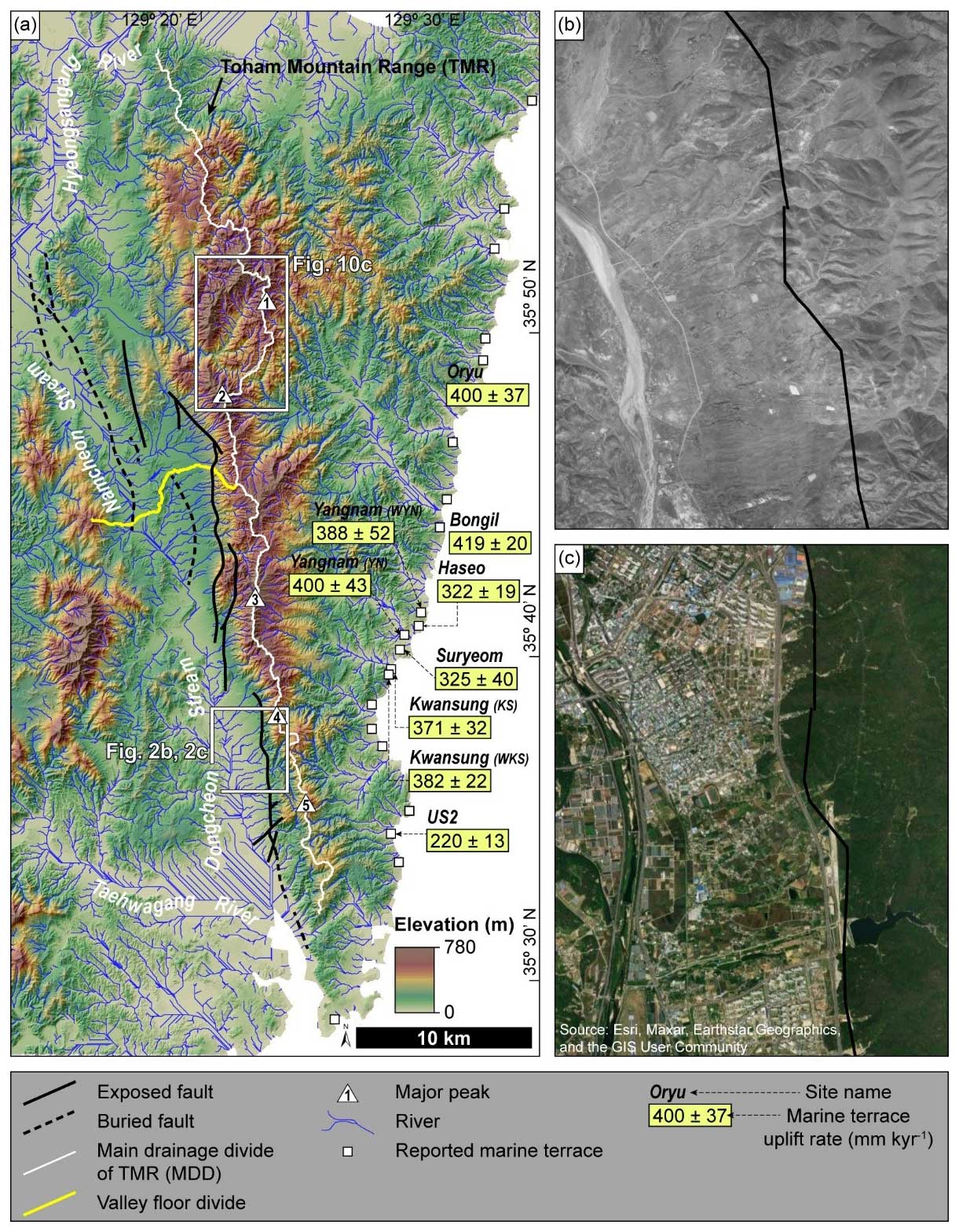
Figure 2 (a) Previously determined uplift rates (in mm kyr⁻¹) of marine terraces near the UFZ, based on the OSL ages of raised beach sediments (details about these rates are in Table 1; Choi et al., 2003a, b; Kim et al., 2007; Heo et al., 2014). The drainage system on the western flank of the Toham Mountain range (TMR) is divided by the valley floor divide (Namcheon and Dongcheon streams). Major peaks in the eastern block of the UFZ are marked by numbers in white triangles (1 is for Mount Hamwol, 2 is for the Toham Mountain, 3 is for Mount Gwanmoon, 4 is for the Dongdae Mountains, and 5 is for Muryong). (b) Aerial photograph taken in 1954 of the area depicted by the white box in Fig. 2a. This aerial photograph was taken prior to urbanization by the industrial complex and residential district in the study area (image source: National Geographic Information Institute of the Republic of Korea). Alluvial fans extend along the western flank of the mountains. The exposed Ulsan Fault (black line) is traced along the boundary between the alluvial fans and the TMR. (c) Recent satellite image (ArcMap™ and Esri) of the same area depicted in Fig. 2b. Urbanization since the 1960s has made it difficult to observe natural landforms in this area.

The Toham Mountain range (TMR) is located on the eastern hanging-wall block of the UFZ and extends parallel–subparallel to the fault zone (Fig. 2a). The TMR includes many peaks, including the mountains at Hamwol (584 m), Toham (745 m), Gwanmoon (630 m), Dongdae (447 m), and Muryong (451 m) from north to south. Rivers draining the TMR are divided into eastern- and western-flank rivers by the main drainage divide (MDD; Fig. 2a). Rivers draining the eastern flank of the TMR flow to the east and drain directly into the East Sea, whereas those on the western flank form a more complex drainage system flowing north or southward from a low-elevation valley floor divide. Western-flank channels are categorized based on their draining into the catchments either north or south of the valley floor divide. Channels in the northern part of the valley floor divide flow to the west and join together to form the Namcheon Stream. The Namcheon Stream flows to the north–northwest and joins other tributaries to form the Hyeongsangang River, which drains into the East Sea. Channels in the southern part of the valley floor divide flow to the west and join to form the Dongcheon Stream, which flows to the south. The Dongcheon Stream joins the Taehwagang River, which drains into the South Sea of the Korean Peninsula. The landscapes of the western and eastern flanks differ significantly from each other; the western flank is dominated by a clearly defined mountain front with extensive alluvial fans (Fig. 2a and b), whereas the eastern flank has broader mountainous and a hilly landscape that extends from the TMR all the way to the eastern coast (Figs. 1a and 2a). The cause of the contrasting landscapes of the western and eastern flanks of the TMR has yet to be unequivocally established, and several explanations have been proposed, including the (1) differential regional rift–margin uplift related to the opening of the East Sea from ca. 20 Ma (Min et al., 2010; D. E. Kim et al., 2016; Kim et al., 2020); (2) differential regional uplift caused by accommodation of the ENE–WSW-oriented neotectonic maximum horizontal stress since 5 Ma (Park et al., 2006; M.-C. Kim et al., 2016); and (3) differences in late Quaternary uplift between the western and eastern coasts of the Korean Peninsula, as recorded in marine terraces along the eastern coast (Choi et al., 2003a, b, 2008, 2009; Lee et al., 2015) and the shore platform along the western coast (K. H. Choi et al., 2012; Jeong et al., 2021). We weigh in on these possibilities using new data sets in this study.

In addition, numerous studies have attempted to elucidate the geological and geomorphic history of the broader southeastern Korean Peninsula. Studies of the UFZ have reported many active faults (Fig. 1b), but age data from those studies need further verification as at present these results lack consensus (Kyung, 1997; Okada et al., 1998, 2001; Cheong et al., 2003; Kim et al., 2021). Furthermore, studies of marine terraces have proposed paleo-shoreline elevations and the optically stimulated luminescence (OSL) ages of beach sediment layers for each terrace sequence (Choi et al., 2003a, b; Kim et al., 2007; Heo et al., 2014). In this study, we calculated the amount of uplift of each terrace, considering local paleo-sea levels and terrace uplift rates (Table 1 and Fig. 2a).

Table 1 Information on previously studied marine terraces within the study area.

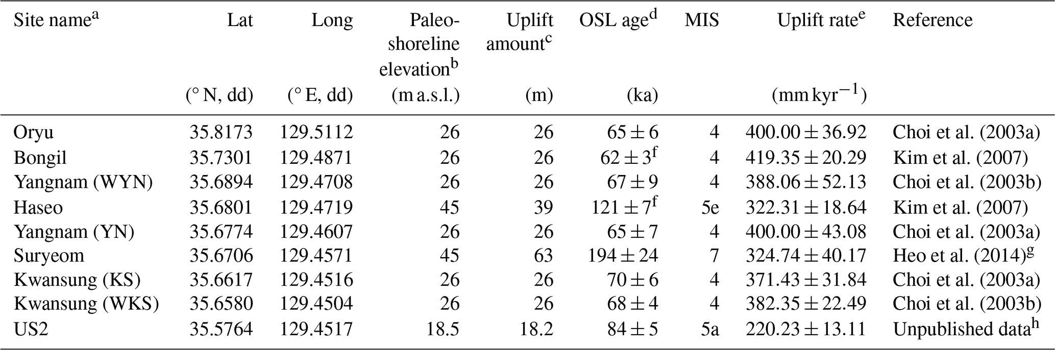
^a The list of sites runs from north to south (Fig. 2a), with some sites sharing names but having different sampling locations (shown in parentheses after affected sites). ^b The paleo-shoreline elevation is the present-day elevation of the paleo-shoreline for each terrace. ^c The uplifted amount is calculated by subtracting the elevation of the sea level at the marine terrace formation from the paleo-shoreline elevation. We considered the elevation of the local sea level of each Marine Isotope Stage (MIS) corresponding to each marine terrace age (Lee et al., 2015; Ryang et al., 2022) in our calculations. ^d Mean ages and 1σ standard deviations are given. These studies used the beach sediment to infer the depositional age. ^e The uplift rate is calculated by dividing the uplifted amount by the age of marine terrace. ^f This age is the average of two samples. ^g This study applied a single-grain OSL dating method, while the other studies applied single-aliquot OSL dating method. ^h Age data are from the big-data open platform (https://data.kigam.re.kr/map/, last access: 14 July 2023) managed by Korea Institute of Geoscience and Mineral Resources (KIGAM). The notation dd refers to decimal degrees.

3 Methods

3.1 Topographic analysis

We used a 5 m resolution digital elevation model (DEM) to extract the following topographic metrics: (1) normalized channel steepness index (k_sn), (2) stream profiles, (3) metrics for assessing drainage divide mobility, and (4) swath profile. These metrics have been widely used to quantitatively measure topography and geomorphic processes across a diverse range of tectonic and climatic settings. We employed these metrics to assess the relative tectonic activity and to delineate geomorphic-based fault segments, although very few additional case studies exist (see, e.g., Lee et al., 2021). The DEM was generated using digital contours provided by the National Geographic Information Institute (NGII) of the Republic of Korea (https://www.ngii.go.kr/kor/main.do; last access: 14 September 2020) and was projected to the World Geodetic System 1984 (WGS 84) Universal Transverse Mercator (UTM) coordinates. We corrected the DEM using the “carving” option of TopoToolbox (Schwanghart and Scherler, 2014) for our analysis, which matches the flow route to the deepest path. Channel initiation is determined by the threshold drainage area of 10⁵ m².

3.1.1 Normalized channel steepness index (k_sn)

A channel under steady-state conditions in which the uplift, climate, and rock resistance are spatially uniform maintains a graded profile, following a power law equation (Hack, 1973; Flint, 1974):

$$\begin{array}{}\text{(1a)}& {\displaystyle }S=k_{\mathrm{s}}{A}^{-\mathit{\theta }}\text{(1b)}& {\displaystyle }S=k_{\mathrm{sn}}{A}^{-{\mathit{\theta }}_{\mathrm{ref}}},\end{array}$$

where θ is the concavity index of a channel or channel reach ($\mathit{\theta }=m/n$). The channel steepness index (k_s) may be changed by the concavity index, and this makes it difficult to compare values of the channel steepness index with those of other channels with different concavity index values and differently sized of drainage basins. To facilitate such a comparison, the normalized channel steepness index (k_sn) can be calculated by fixing the concavity index to a reference value (θ_ref) in the range of 0.36–0.65 (Snyder et al., 2000; Wobus et al., 2006; Cyr et al., 2010; Kirby and Whipple, 2012). However, many streams in nature are not graded, particularly if they have undergone base level changes that resulted from climate change (Crosby and Whipple, 2006), tectonic forcing (Snyder et al., 2000; Kirby and Whipple, 2001), or lithological differences (Cyr et al., 2014). Such streams show peaks or piecewise-fitted lines in a log S–log A plot and display an abrupt variation in k_sn along their course, indicating that they are in a transient geomorphic state. We computed k_sn as the derivative of χ and elevation, as noted by Eq. (2a), with θ_ref of 0.45, using LSDTopoTools (Mudd et al., 2014). To validate the use of the empirical value we use, we calculated concavity indices across the study area, which ranged from 0.36 to 0.47. Therefore, we believe that using 0.45 as θ_ref should not pose any major issues.

3.1.2 Stream profile analysis and knickpoint extraction

According to Eq. (1a), a graded stream has a concave longitudinal profile and is represented as a single line on a log S–log A plot. The χ-transformed stream profile of a graded stream (χ−z plot) would also be represented by a single line, based on Eq. (2a). However, rivers in transient states are expected to show several piecewise linear segments in χ-transformed stream profiles (Perron and Royden, 2013). The boundary between adjacent piecewise lines can be identified as knickpoints, which are the parts of a channel with abrupt changes in the slope and elevation of the channel beds. A knickpoint can reflect the transient state of a stream caused by a base level change related to climatic change (Crosby and Whipple, 2006), tectonic forcing (Snyder et al., 2000; Kirby and Whipple, 2001), or lithological differences (Cyr et al., 2014).

We used TopoToolbox (Schwanghart and Scherler, 2014) to extract the longitudinal stream profiles. To visualize the changes in the normalized channel steepness index values more easily, we extracted χ-transformed stream profiles, using LSDTopoTools (Mudd et al., 2014). This tool employs an algorithm to analyze the best-fitting piecewise line for each channel segment (Mudd et al., 2014).

We set the reference concavity index (θ_ref) to 0.45 and the reference scaling area (A₀) to unity for integral transformation of χ the coordinate.

3.1.3 Metrics for assessing drainage divide mobility

Drainage divide mobility is determined by contrasts in the erosion rates of the adjacent drainage basins. As the erosion rates depend on topography, we can use topographic metrics to assess the divide mobility and drivers of the divide migration. We used the mean upstream relief, which is the most reliable metric among the Gilbert metrics (Forte and Whipple, 2018), and the χ index to evaluate topographic asymmetry and divide mobility. This is based on the “law of divides” of Gilbert (1877), which suggested that the steeper slope is expected to be eroded and reduced in height more rapidly when compared with the gentle slope (Fig. 70 in Gilbert, 1877). The migration will in principle continue until the two sides become symmetric (geometric equilibrium) (Gilbert, 1877). In addition to these metrics, the chi (χ) index at opposing channel heads can also be used to evaluate the long-term divide stability (Willett et al., 2014; Forte and Whipple, 2018). The χ index at point x on the channel serves as a proxy for the steady-state elevation of the channel and is calculated by integrating Eq. (1b) from downstream to upstream as follows (Perron and Royden, 2013):

$$\begin{array}{}\text{(2a)}& {\displaystyle }z\left(x\right)=z_{\mathrm{b}}+\left({\displaystyle \frac{k_{\mathrm{sn}}}{A_{\mathrm{0}}^{{\mathit{\theta }}_{\mathrm{ref}}}}}\right)\mathit{\chi },\text{(2b)}& {\displaystyle }\mathit{\chi }=\underset{x_{\mathrm{b}}^x}{\int }{\left({\displaystyle \frac{A_{\mathrm{0}}}{A\left(x{}^{\prime }\right)}}\right)}^{{\mathit{\theta }}_{\mathrm{ref}}}\mathrm{d}{x}^{\prime },\end{array}$$

where x is the distance upstream from an arbitrary base level, z_b is a base level elevation (at x=x_b), A₀ is an arbitrary scaling area, and A(x) is the drainage area at point x on the channel. The integrand in Eq. (2b) becomes dimensionless, meaning that the χ index can be expressed with a unit of length (Perron and Royden, 2013). Equation (2a) establishes the linear relationship between the elevation and the χ index when the rock uplift, bedrock erodibility, and climate conditions are invariant along the channel, and the χ index is calculated with the adequate θ_ref. If such boundary conditions vary spatially, then the elevation and χ index will have a piecewise–linear relationship. The scaling area, A₀, is set to unity, as the slope of the χ index–channel elevation plot (χ−z plot) is equal to k_sn, based on Eq. (2a). We used the TopoToolbox (Schwanghart and Scherler, 2014) and DivideTools (Forte and Whipple, 2018) to analyze the mean upstream relief and the χ index. The mean upstream relief was calculated within a radius of 200 m, which was determined by considering the resolution of topographic data and the distance between the channel head and MDD. Finally, because the χ index is sensitive to the base level elevation (z_b; Forte and Whipple, 2018), we analyzed the χ index with two different base level elevations (50 and 200 m). Drainage basins with base level elevations lower than 50 m and higher than 200 m do not adequately describe the variation in the topographic metrics along the UFZ. For these basins, we performed Student's t tests, which are statistical methods used to determine whether two groups are statistically significantly different from each other. We applied this Student's t test (two-tailed; α=0.05) to statistically compare the values of these topographic metrics between the western and eastern flanks of the TMR.

3.1.4 Swath profile

Swath profiles quantify how the minimum, mean, and maximum elevation varies across a region along a profile. They have proven useful to understand the relationship between the surface topography (i.e., the swath profiles) and associated or causative variables, such as dynamic topography, which is a topographic change caused by mantle convection (Stephenson et al., 2014), or spatial variations in precipitation (Bookhagen and Burbank, 2006), uplift, and exhumation rates (Taylor et al., 2021). We extracted a swath profile along the MDD by setting the width to 3 km using TopoToolbox (Schwanghart and Scherler, 2014) as the along-strike topographic variation is expected to be related to the along-strike variation in the cumulative vertical displacement on the UFZ.

3.2 In situ cosmogenic ¹⁰Be measurements

Assuming that a channel of interest approaches a topographic steady-state where the channel bed maintains a constant elevation due to the balance between uplift and incision, an uplift rate can be derived from the bedrock channel incision rate (Eqs. 1 and 2). We used in situ cosmogenic ¹⁰Be measurements to constrain the catchment-averaged denudation rate, as well as bedrock channel incision rates, to quantify the uplift rates and the stream power variations controlled by tectonic uplift in our study area.

3.2.1 Catchment-averaged denudation rate

The concentration of in situ cosmogenic ¹⁰Be from riverine sediment on the present bedrock channels can be interpreted as the catchment-averaged denudation rate (CADR). This approach assumes a geochemical steady state whereby the production and removal (via denudation) rates of cosmogenic ¹⁰Be within the catchment are equal (Brown et al., 1995; Bierman and Steig, 1996; Granger et al., 1996; von Blanckenburg, 2005). Thus, the CADR represents the average denudation rate across the entire catchment by hillslope and fluvial processes over a given integration time, during which the sediments remained within the catchment (Granger et al., 1996; von Blanckenburg, 2005). The integration time documented in previous studies from a variety of tectonic, climatic, and topographic environments varies from 10³ to 10⁶ years (Brown et al., 1995; DiBiase et al., 2010; Portenga et al., 2015; Kim et al., 2020).

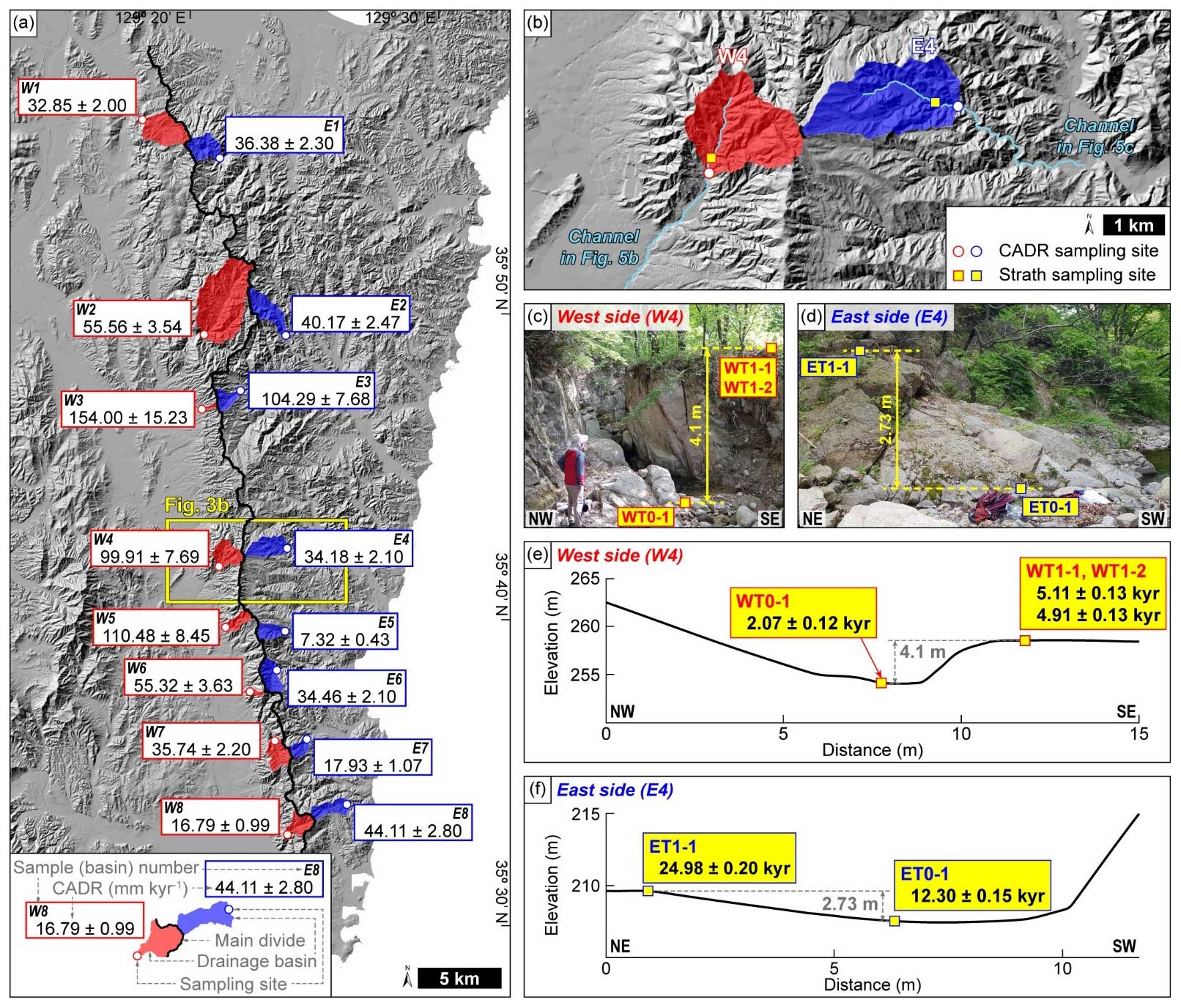
Figure 3 Sampling sites and results of catchment-averaged denudation rates (CADRs) and channel incision rates derived from in situ cosmogenic ¹⁰Be measurement. (a) CADRs calculated using in situ cosmogenic ¹⁰Be measurements and their sampling sites. We collected samples for ¹⁰Be analysis and CADR calculation from eight pairs of basins (16 basins) along the main drainage divide. CADR values on the western flank of the TMR (shown in red) are mostly higher than those on the eastern flank (shown in blue). (b) Bedrock strath sampling sites, where channel profiles are provided in Fig. 5b and c, are marked. (c, d) Photographs of the bedrock strath sampling sites on the western and eastern flanks of the TMR, respectively. We collected samples from the bedrock strath and the present stream bed in the same catchments from which we collected samples W4 and E4 for CADR calculation. The height of the western-flank strath above the present stream bed is 4.1 m, and the height of the eastern-flank strath above the present stream bed is 2.73 m. (e, f) Elevation profiles across the bedrock strath sampling sites and their ¹⁰Be exposure ages on the western and eastern flanks of the TMR, respectively. The age difference between the present stream bed and the strath is 2.94±0.15 kyr on the western flank and 12.68±0.25 kyr on the eastern flank. The discrepancy between CADR and the bedrock channel incision rate is tentatively caused by (1) the difference between the integration time of CADR and the exposure age of the strath surface and by (2) the difference in the spatial scales which is represented by those two methods.

We collected 16 samples of riverine sediment from 8 pairs of catchments (a total of 16 catchments) straddling both sides of the MDD of the TMR (Fig. 3a) to document variations in the CADR along the MDD. More specifically, we aim to compare the CADRs of the western and eastern flanks of the TMR to reveal the direction of divide migration and tectono-geomorphic history of the hanging-wall and footwall blocks. The along-MDD variation and across-MDD contrasts were subsequently compared with results from our topographic analysis to characterize tectonic activity and spatial variability along the UFZ. We obtained samples of fine- to medium-grained sand (250–500 µm) from channel beds. To prevent possible contamination by anthropogenic debris, we avoided collecting samples from catchments containing golf courses and areas downstream from alluvial fans and where known faults occur (Fig. 2). The lithology of the sampled catchments includes mainly sedimentary rocks and igneous rocks of various geological ages (Fig. 1b). The lithology within each pair of basins (basins contacting at the MDD, such as basins W1 and E1 in Fig. 3a) is, however, highly similar, ensuring a minimal influence of the lithological difference on CADRs for comparison in the across-MDD direction. However, some lithological variations do occur in the along-MDD direction. The basins W1 and E1 consist of rhyolite and dacite bedrock. Basins W2, W3, E2, and E3 contain rhyolite, dacite, and granite bedrock, as shown in Fig. 1b. The remaining basins (W4–W8 and E4–E8; eight basins) contain sedimentary, volcanoclastic, and granite bedrock.

We performed chemical treatment of the CADR samples at Korea University, Seoul, South Korea, following standard protocols for ¹⁰Be extraction (Kohl and Nishiizumi, 1992; Seong et al., 2016). We leached the samples with a HCl–HNO₃ mixture to remove organic and carbonate materials. Then, we used a HF–HNO₃ mixture to remove minerals other than quartz and meteoric ¹⁰Be adsorbed onto the surface of mineral particles. A total of 15–20 g of pure quartz was yielded after separating magnetic minerals and picking out other impurities. A ⁹Be carrier with a low background level of ¹⁰Be was then added to the samples, which were then dissolved with a high-concentration HF–HNO₃ mixture. We extracted beryllium using an ion-exchange column, precipitated it into BeOH, dried the BeOH gel, and calcined it into BeO. Samples in the BeO form were mixed with niobium powder and targeted into the cathode of the accelerator mass spectrometer (AMS), where measurements were performed at the Korea Institute of Science and Technology (KIST), Seoul, South Korea. Measured ¹⁰Be $/$ ⁹Be results were normalized to the 07KNSTD reference 5-1 sample (Nishiizumi et al., 2007) and calculated as ¹⁰Be concentrations after correction with a process blank (4.37–$\mathrm{4.53}\times {\mathrm{10}}^{-\mathrm{15}}$; n=6).

We utilized the Basinga (basin-averaged scaling factors, cosmogenic production, and denudation rates) tool (Charreau et al., 2019) to calculate CADRs and the integration time from ¹⁰Be concentrations. This tool calculates the basin-averaged production rate of in situ cosmogenic ¹⁰Be from every cell of a DEM, based on its location. The tool requires raster files of a DEM and offers scaling schemes of Lal–Stone (Lal, 1991; Stone, 2000), LSD and LSDn (Lifton et al., 2014), along with geomagnetic correction based on the virtual dipole moment (Muscheler et al., 2005). We used the same topographic data for calculating CADRs as we did for topographic analysis, employing a 5 m resolution DEM derived from digital contours of NGII. Additionally, we applied the LSDn scaling scheme (Lifton et al., 2014) and geomagnetic correction (Muscheler et al., 2005).

3.2.2 Bedrock channel incision rate

The classical model for fluvial strath terrace formation includes the widening of the terrace tread by lateral erosion and its abandonment by incision (Burbank and Anderson, 2011). Each abandoned terrace thus represents the position of the paleo-channel of the stream bed, and the bedrock incision is controlled by uplift, as channels incise bedrock while they attain a steady state. If the concentration of in situ cosmogenic ¹⁰Be on a strath surface can be measured, then the exposure age of that bedrock strath can be calculated, indicating the time elapsed since the abandonment of the strath surface.

We collected three samples from western-flank straths and two from eastern-flank straths (Fig. 3) to constrain the exposure age of each tread. The sampled strath terraces are located in the drainage basin from which the W4 and E4 CADR samples were taken. All terraces are developed on granite bedrock. The height of the strath terrace from the channel bed on the western flank was 4.10 m, and that on the eastern flank was 2.73 m (Fig. 3c–f). On the western flank, the valley is deep and narrow, and the valley wall is steep. On the eastern flank, the valley is wide and gentle, and the exposed valley wall and terrace riser are more weathered than those on the western flank. The terraces in both valleys are unpaired.

Following the same laboratory protocol described above (Kohl and Nishiizumi, 1992; Seong et al., 2016), we performed a physical and chemical treatment for in situ surface exposure dating samples at Korea University, Seoul, South Korea. We crushed bedrock samples using a jaw crusher and iron mortar and separated fine- to medium-sized sand (250–500 µm) grains by sieving. The further chemical treatments were the same as those applied to our CADR samples (see Sect. 3.2.1). AMS measurements were made at Korea Institute of Science and Technology (KIST), Seoul, South Korea. We calculated exposure ages using the CRONUS-Earth online calculator (Balco et al., 2008; version 3.0.2), applying the LSDn scaling scheme (Lifton et al., 2014). Uncertainties in the exposure ages were calculated and are given as 1σ values.

3.3 Landscape evolution modeling

We applied the open-source landscape evolution model toolkit called Landlab (Hobley et al., 2017; Barnhart et al., 2020; Hutton et al., 2020) to investigate specific landscape evolution model setups to gain insight into the evolution of the uplifted eastern hanging-wall block of the UFZ. These simulations were then compared with results from our topographic analyses and ¹⁰Be measurements to interpret the landscape evolution of the study area. We considered two processes that erode topography and transport sediment, namely (1) fluvial erosion and (2) hillslope diffusion.

The bedrock channel incision rate, E, can be expressed by Eq. (3), which describes its relationship with channel bed shear stress as follows (Howard and Kerby, 1983; Seidl and Dietrich, 1992; Sklar et al., 1998):

$$\begin{array}{}\text{(3)}& E=K{A}^m{S}^n,\end{array}$$

where K is a dimensional coefficient of fluvial erosion efficiency with a unit of [L^1–2 m T⁻¹] encapsulating different controls on erosion, such as rock resistance, climate, bedload sediment grain size, and channel width–length relationship (Stock and Montgomery, 1999; Whipple and Tucker, 1999, 2002; Snyder et al., 2000). A [L²] is the drainage area. S [L L⁻¹] is the slope. m and n are exponents of drainage area and slope, respectively. We used values of $K=\mathrm{5.56}\times {\mathrm{10}}^{-\mathrm{7}}$ m^−1.29 yr⁻¹, m=1.1448, and n=2.2896 to simulate fluvial erosion, which was estimated by averaging values calculated for regions with similar lithology, climate, and tectonic activity to those of our study area (Harel et al., 2016). We applied an incision threshold of $\mathrm{1.0}\times {\mathrm{10}}^{-\mathrm{5}}$ m yr⁻¹, below which no incision is assumed to occur (Tucker and Whipple, 2002; Harel et al., 2016; Hobley et al., 2017).

Topographic change caused by hillslope diffusion is controlled by the diffusion equation as (Culling, 1963; Tucker and Bras, 1998)

$$\begin{array}{}\text{(4)}& {\displaystyle \frac{\partial z}{\partial t}}=K_{\mathrm{d}}{\mathrm{\nabla }}^{\mathrm{2}}z,\end{array}$$

where K_d is the coefficient of diffusivity with a unit of [L² T⁻¹]. ∇² is the Laplace operator, which is the divergence of gradient. z is elevation. We used K_d=0.001 to simulate the hillslope diffusion process, which we adopted because soil is rare on slopes (Fernandes and Dietrich, 1997; Zebari et al., 2019).

A landscape's gain in height by tectonic uplift and loss of height by fluvial erosion and hillslope diffusion can be expressed as (Temme et al., 2017)

$$\begin{array}{}\text{(5)}& {\displaystyle \frac{\partial z}{\partial t}}=U-K{A}^m{S}^n-K_{\mathrm{d}}{\mathrm{\nabla }}^{\mathrm{2}}z.\end{array}$$

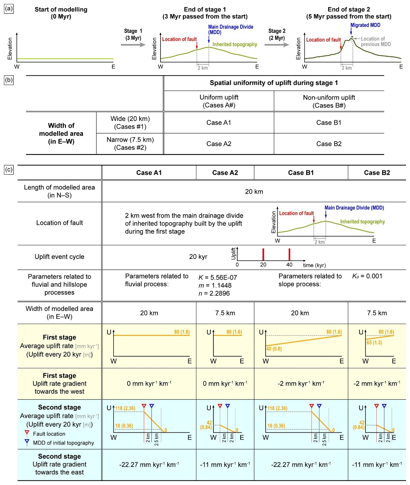
Figure 4 Diagram showing the configuration of the landscape evolution model (LEM) used to simulate the tectono-geomorphic evolution of the eastern hanging-wall block of the UFZ. (a) The two stages of the LEM. Stage 1, corresponding to a duration of 3 Myr, involves simulation of building of the initial topography; i.e., the topography prior to reverse faulting of the UFZ during the Plio-Quaternary. Stage 2, corresponding to a duration of 2 Myr, involves the simulation of reverse faulting and associated neotectonic surface uplift on the UFZ during the Quaternary. We modeled the location of the fault in the LEM as being 2 km west of the average location of the main drainage divide (MDD) of the initial topography. (b) The four model cases (A1–A2 and B1–B2) used to test different conditions of spatial uniformity/non-uniformity of uplift during stage 1 and the width of the modeled domain. (c) Detailed settings for each case (A1–A2 and B1–B2) of the LEM. The settings in the first four rows of this table are universal to all four cases. We applied different uplift rates and spatial gradients in uplift during both stages 1 and 2 for each case. “U” means average uplift rate (in units of mm kyr⁻¹), “W” means the western boundary of the eastern block of the UFZ, and “E” means the eastern boundary of the eastern block of the UFZ. The numbers in the parentheses represent the uplift amounts every 20 kyr (i.e., one uplift event cycle). Model uplift rate during stage 1 for Cases A1 and A2 is spatially uniform, whereas that for Cases B1 and B2 is spatially variable, decreasing linearly from east to west. In the second-to-last row of the table, the red triangle denotes the location of the fault, and the blue triangle marks the location of the MDD of initial topography. The uplift rate during stage 2 decreases linearly with increasing distance from the fault. The uplift rates and their spatial gradient during stage 2 depend on the width of the modeled domain. Cases labeled 1 share the same uplift rate and its spatial gradient, and cases labeled 2 have the same values for the uplift rate and its spatial gradient.

We designed the landscape evolution model to encapsulate two stages. The first establishes the inherited topography, and the second simulates that related to the reverse fault reactivation (Fig. 4a). By applying different boundary conditions during the first stage (Fig. 4b), we could simulate various inherited topographies. This approach allowed us to test our hypothesis that inherited topography can significantly influence the present landscape and our observed patterns of topographic metrics. The first stage is a pre-Quaternary period during which initial topography is built; i.e., this refers to the topography that already existed before reverse faulting of the UFZ during the Quaternary. This period simulates the regional uplift prior to the Quaternary reverse fault reactivation of the UFZ. The second stage is a period used to simulate local uplift by reverse faulting, representing the neotectonic movement of the UFZ during the Quaternary. In the model, we structured stage 1 to last for 3 Myr and stage 2 to last for 2 Myr, giving a total time of 5 Myr. The total duration corresponds to the duration of the present stress regime, as the regional and local uplift both occurred under the present stress regime (Park et al., 2006; M.-C. Kim et al., 2016).

With this model structure, we tested four cases differentiated by varying two parameters: (1) the spatial uniformity of the uplift rate in the first stage and (2) the width of the modeled domain (Fig. 4b). First, the cases can be separated into two groups (A and B) based on the spatial uniformity of uplift rate during stage 1. The cases simulating a spatially uniform uplift rate during stage 1 (henceforth “Cases A#”) assume no spatial gradient in the uplift rate; i.e., the whole eastern block of the UFZ underwent uniform uplift during stage 1. The cases simulating a spatially variable uplift rate during stage 1 (henceforth “Cases B#”) assume a spatial gradient in the uplift rate whereby the eastern side of the block was uplifted more than the western side (i.e., the modeled domain tilted westward). This assumption is based on the overall tendency of the high-east and low-west topography of the Korean Peninsula, supported by the long-term regional westward tilting that was initiated during the middle Miocene when the East Sea started to widen and since the time during which the strongly asymmetric (high-east) Taebaek Mountain range has been rapidly uplifted (Min et al., 2010; Kim et al., 2020). In addition, the shore platform on the western coast of the peninsula (0 m a.s.l.; K. H. Choi et al., 2012; Jeong et al., 2021) and marine terraces along the eastern coast (18–45 m a.s.l.; Choi et al., 2003a, b; Kim et al., 2007; Heo et al., 2014; Lee et al., 2015) formed at the same time (i.e., during MIS 5), indicating that regional differential uplift of the entire peninsula has lasted until very recently. Second, we divided the cases into two groups (henceforth “Cases #1 and #2”), based on the width of the modeled domain (Fig. 4b), to simulate the observation that the eastern block of the UFZ is wide at its northern extent and narrows towards the south (Fig. 1). The width of the wide-model domain (measured in an E–W direction) is 20 km (henceforth “Cases #1”) and that of the narrow-model domain (henceforth “Cases #2”) is 7.5 km, so that Cases #1 and #2 represent the northern and southern parts of the block, respectively.

In all four cases, we employed identical values for the following settings and parameters: (1) the length of the modeled domain in the N–S direction, (2) the location of the fault, (3) the parameters used to simulate fluvial and hillslope processes, and (4) the uplift event cyclicity (Fig. 4c). The N–S length of the modeled domain was set to 20 km for all cases. We positioned the model of Ulsan Fault 2 km west of the average location for the MDD in the initial topography (Fig. 4a and c). This was done because the present-day location of the UFZ is approximately 2 km west of the MDD in the eastern block. The three parameters associated with fluvial process, namely the coefficient of erosion (K) and exponents of area (m) and slope (n), and the one parameter associated with slope processes, namely, the coefficient of diffusivity (K_d; as described above; Fig. 4c), were set to constants. Finally, we set the uplift event cyclicity (i.e., the duration between discrete faulting and uplift events) to 20 kyr. Although the earthquake recurrence interval has not yet been definitively determined for the Ulsan Fault, we used a realistic value based on the correlation between the earthquake magnitude, recurrence interval, and geomorphic evidence proposed by Slemmons and Depolo (1986), as well as the timing of the most recent and penultimate earthquakes in the study area (Cheon et al., 2020a; T. Kim et al., 2023).

We applied different average uplift rates and associated spatial gradients during both stages for the individual cases we explore (Fig. 4c). The average uplift rates during stage 1 for Cases A1 and A2 were spatially uniform (i.e., no spatial gradient). The average uplift rate for Cases A# during stage 1 was set to 80 mm kyr⁻¹. This value was chosen to set our model uplift rate to be the same as the long-term (from 22 Ma until today) exhumation rate across the Taebaek Mountain range (the “backbone” mountain range of the Korean Peninsula) (Han, 2002; Min et al., 2010; D. E. Kim et al., 2016). Conversely, Cases B1 and B2 incorporate a spatial gradient in uplift rate, with the highest uplift rate in the east, decreasing gradually towards the west during stage 1. Although the spatial gradient of uplift rate is uncertain, we chose to model the average uplift rate at the western margin of the domain in Case B1 (40 mm kyr⁻¹) as half of the maximum uplift rate at the eastern margin (80 mm kyr⁻¹), which is equivalent to the uplift rate of Cases A# during stage 1 (Fig. 4c). The same spatial gradient in the uplift rate (−2 mm kyr⁻¹ km⁻¹) was applied in Case B2.

During stage 2 (Quaternary reverse faulting), the average uplift rate is set to be the highest in the location of the fault and to diminish linearly with increasing distance from the fault. To determine the maximum vertical displacement per event, we assumed that a maximum earthquake magnitude of M_W 7.0 occurs once per 20 kyr (Slemmons and Depolo, 1986; Kyung, 2010), although different maximum magnitude estimates (M_W 4.6–5.6) have been proposed for the Ulsan Fault (Choi et al., 2014). According to the empirical equation of Moss and Ross (2011), a M_W 7.0 earthquake would generate a maximum vertical displacement of approximately 2.36 m. Therefore, we hypothesized a scenario in which a M_W 7.0 earthquake produces a maximum vertical displacement on the fault of 2.36 m every 20 kyr. Under this scenario, the average long-term surface uplift rate at the fault location for Cases #1 is 118 mm kyr⁻¹ (0.118 mm yr⁻¹), as calculated by dividing the maximum vertical displacement (2.36 m) by 20 kyr (Fig. 4c). This rate decreases linearly to 18 mm kyr⁻¹ (0.018 mm yr⁻¹) at a distance of 2.5 km east of the MDD of the initial model topography. This value (18 mm kyr⁻¹) is calculated by multiplying the average uplift rate at the fault location (118 mm kyr⁻¹) by the ratio of the eastern-flank channel incision rate (215 mm kyr⁻¹) to that in the west (1394 mm kyr⁻¹). This calculation reflects the fact that the sampled western-flank strath is located ∼2 km west of the UFZ, and the eastern-flank strath we sampled is ∼2.5 km from the MDD. For Cases #2, representing the southern part of the block, we applied a lower average uplift rate of 42 mm kyr⁻¹ (0.042 mm yr⁻¹) at the fault (Fig. 4c). We used this lower uplift rate because CADRs in the southern part of the study area are lower than those in the northern part (Table 2 and Fig. 3a). This uplift rate (42 mm kyr⁻¹) was calculated by multiplying the ratio of the average CADR of W6–W8 (36.25 mm kyr⁻¹) to the CADR of W4 (100.56 mm kyr⁻¹) by 118 mm kyr⁻¹. This choice in the parameterization reflects that the western-flank strath terrace is located within the drainage basin from which we collected the W4 CADR sample. The uplift rate becomes zero 2 km east of the MDD because most of the knickpoints on the eastern-flank channels in the southern part of the study area are located within 2 km of the MDD (Fig. 5a).

Each of the four landscape evolution model cases has a grid spacing of 100 m. We traced the change in the topography development using a time step of 100 years. Comparisons between the resultant topographies from Case A1 to Case B1 and from Case A2 to Case B2 allow us to detect the influence of inherited topography (i.e., topography achieved after stage 1) on the subsequent geomorphic response to the same pattern of tectonic movement (i.e., uplift by faulting during stage 2). Similarly, comparisons of the resultant topographies from Case A1 to Case A2 and from Case B1 to Case B2 enable us to detect the differential geomorphic response controlled by differences in the width of the modeled domain or in channel length. In addition, our model results can be used to compare our results obtained from topographic analysis, CADRs, and channel incision rate calculation from ¹⁰Be measurement, as these were used as inputs for the simulation. We analyzed mean upstream relief and the χ index for the model topographies using TopoToolbox (Schwanghart and Scherler, 2014) and DivideTools (Forte and Whipple, 2018) to quantitatively compare the topographies generated in the four cases.

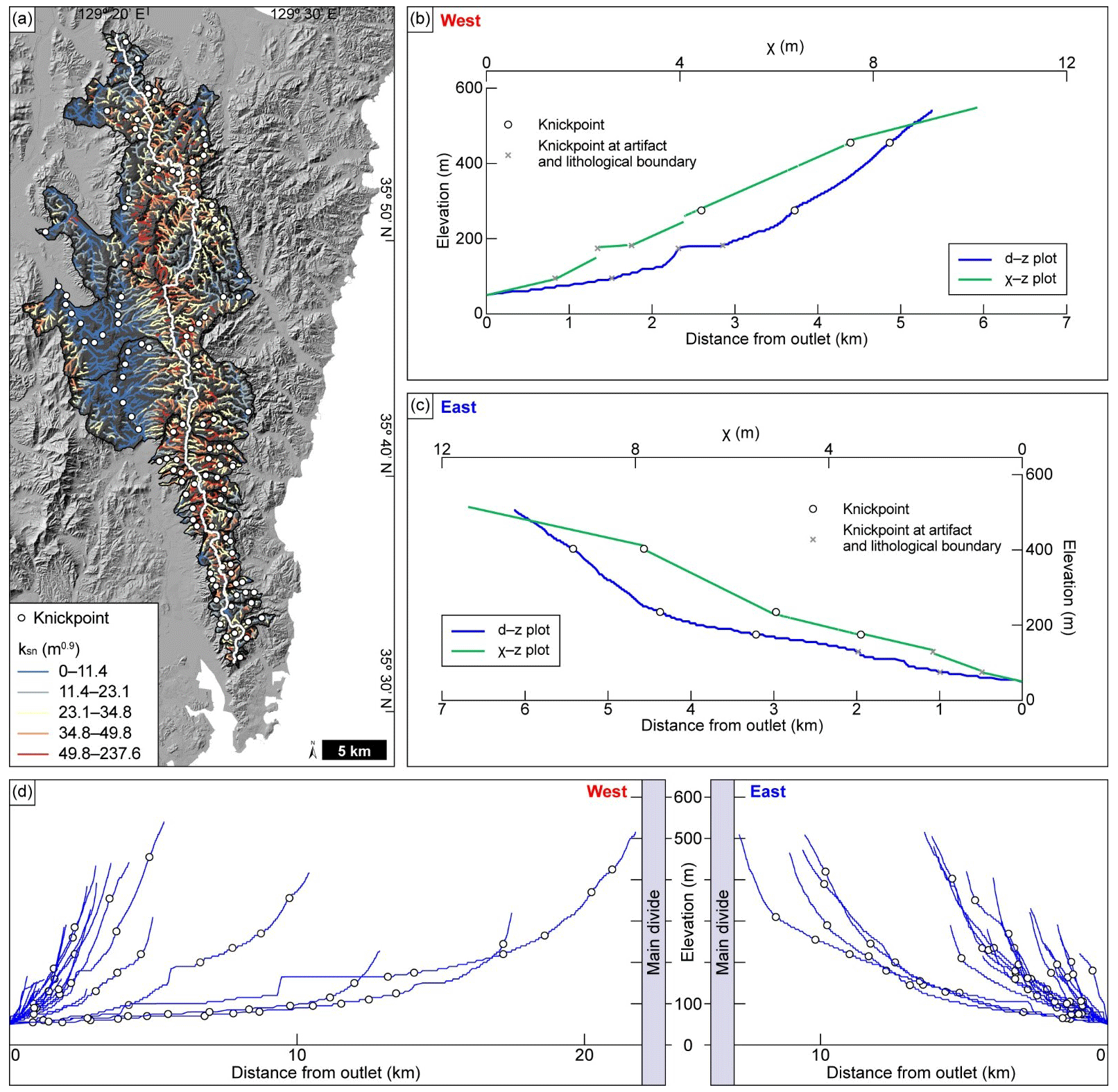
Figure 5 (a) Spatial distribution of knickpoints on trunk stream channels and a map of the normalized steepness index (k_sn) for the entire study area. A reference concavity index (θ_ref) of 0.45 was applied to calculate values of k_sn. Knickpoints (white circle) were detected after excluding artifacts and lithological boundaries. (b, c) Plots of d–z (blue) and χ–z (green) for a stream on each of the western and eastern flanks, respectively, where d is distance from the outlet, and z is elevation. Knickpoints detected at artifacts and lithological boundaries are marked with grey crosses. The locations of these channels are marked in Fig. 3b. (d) Longitudinal profiles and knickpoints of all trunk channels in the study area. Knickpoints detected at the artifacts and lithological boundaries are excluded.

4 Results

4.1 Topographic analysis

4.1.1 k_sn and knickpoint analyses on stream profiles

We find that k_sn varies from 0 to 238 m^0.9, with a regional mean of 24 m^0.9 and a standard deviation of 16 m^0.9. Values lower than the regional mean k_sn are observed in the lowlands in the incised valley to the west of the MDD. Values higher than the regional mean k_sn appear in the foothills and in the hanging-wall mountain range. Analyses of k_sn and knickpoints on the longitudinal and χ-transformed stream profiles show that the channels on both (western and eastern) sides of the MDD are in a transient state (Fig. 5). This result implies that these channels have been disturbed either by lithologies with different K values or by base level changes. We manually excluded artifact knickpoints (e.g., known anthropogenic features such as dams and reservoirs) and lithological boundaries by examining satellite images and geological maps and performing field checks. The remaining knickpoints are interpreted as being caused by tectonic events, in accordance with the findings of a previous study (D. E. Kim et al., 2016), which suggested, on the basis of a 1-D model, that the observed major knickpoints in the study area are unable to have formed by the sea level changes known to have occurred after the global Last Glacial Maximum.

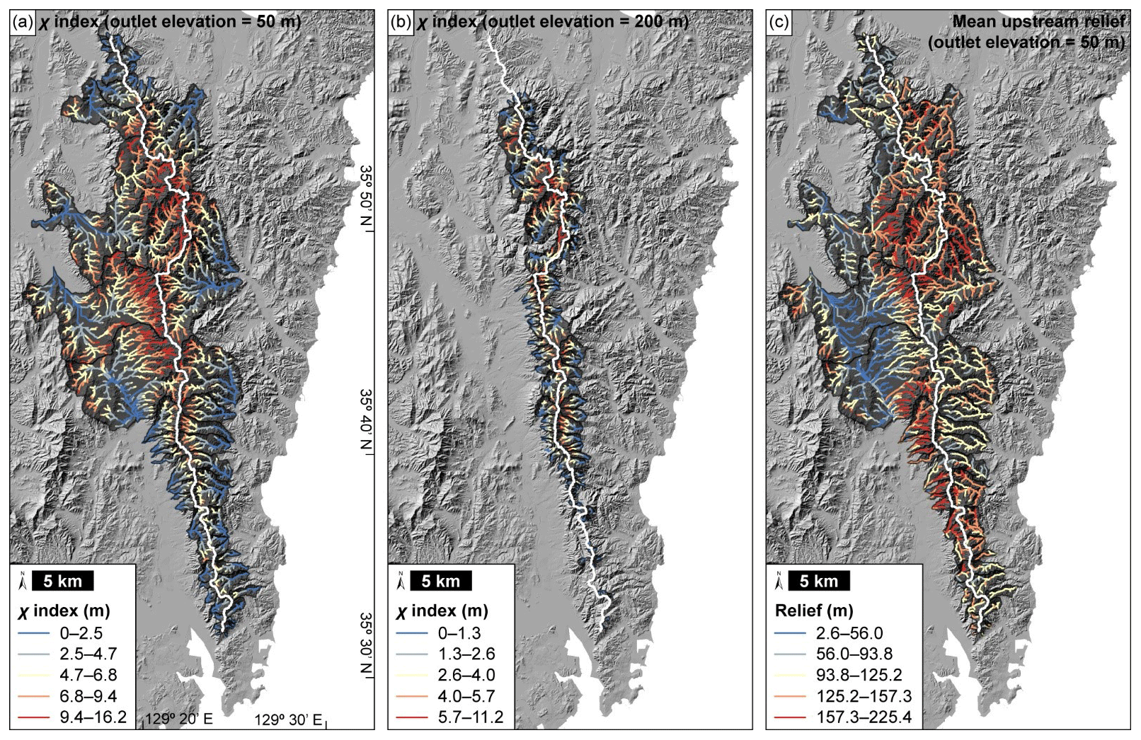
Figure 6 (a, b) Variations in χ index values analyzed with base level elevations of 50 and 200 m, respectively. A reference concavity index (θ_ref) value of 0.45 was applied, and the reference drainage area (A₀) was set to unity for calculation. χ index values at channel heads on the western flank are higher than those on the eastern flank in the northern part of the study area, whereas the χ indices on the eastern flank are higher than those on the western flank in the southern part of the study area. (c) Mean upstream relief calculated within a radius of 200 m. Relief values at channel heads are mostly higher on the western flank than those at the channel heads on the eastern flank.

4.1.2 Variations in values of topographic metrics in the along- and across-MDD directions

We next plotted our topographic metrics analysis results (Fig. 6) to determine whether and, if so, how these metrics vary along and across the MDD (Fig. 7). The along-MDD variation in each topographic metric clearly shows relatively high and low values. The swath profile shows that the highest peak is around 42 km on the horizontal axis, and relatively high peaks also occur at around 25, 51, and 60 km (Fig. 7a). The western k_sn with a base level elevation of 50 m shows the highest value at 59–70 km along the horizontal axis. The segment with a base level elevation of 200 m has the higher values at around 43 and 59–70 km on the horizontal axis. The western mean upstream relief with a base level elevation of 50 m exhibits high values at around 65 and 72–80 km in distance, and the segment with a base level elevation of 200 m has higher values at distances of around 43 and 63 km. Last, the western χ index with a base level elevation of 50 m shows its highest peak at around 41–50 km on the horizontal axis, and the segment with a base level elevation of 200 m has a relatively small variation along the MDD but shows the higher values 32–42, 53, and 60 km of horizontal axis.

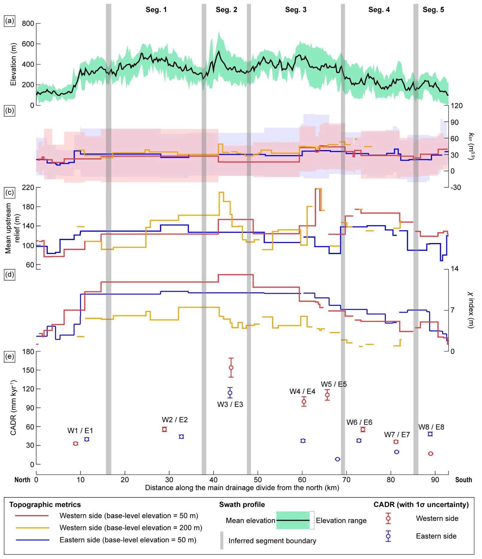
Figure 7 Variation in each topographic metrics along the MDD and fault segmentation proposed for the UFZ. (a) Swath profile along the MDD with an area width of 3 km centered on the MDD. The green-shaded area represents the minimum to maximum elevation. (b–d) Western topographic metrics extracted with a base level elevation of 50 m are represented by a solid red line, those extracted with a base level elevation of 200 m are represented by a solid orange line, and eastern topographic metrics extracted with a base level elevation of 50 m are represented by a solid blue line. (b) Catchment-averaged k_sn. The 1σ uncertainties in the k_sn values extracted with the base level elevation of 50 m on the western and eastern flanks are marked with the red- and blue-shaded areas, respectively. (c) Mean upstream relief at channel heads. (d) Mean χ index at channel heads. (e) Catchment-averaged denudation rate (CADR). Red and blue symbols represent the western and eastern) CADRs of each sample, along with their 1σ uncertainty.

There are some statistically significant differences in topographic metrics between those for the western and eastern flanks along the MDD (Fig. 7). The χ values contrast significantly across the MDD at a distance of 60 km; that of the western flank is 127 % higher than that of the eastern flank between 0–60 km, whereas the χ index values between the western and eastern flanks do not show a significant difference at distances between 60–90 km (Fig. 7). Values of k_sn for the eastern-flank channels are up to 200 % higher than those for the western-flank channels within the 0–60 km section, whereas those for the western-flank channels are up to 137 % higher than those for the eastern-flank channels within the 60–90 km section (Fig. 7). We suggest that these differences arise from fault segmentation.

4.2 In situ cosmogenic ¹⁰Be

4.2.1 Variation in CADR within the study area

CADRs on the western flank range from 16.89±1.00 to 155.23±15.35 mm kyr⁻¹, and those on the eastern flank range from 7.35±0.43 to 104.85±7.71 mm kyr⁻¹ (Table 2 and Fig. 3a). The integration times of these denudation rates cover the interval range of 4.5–95 kyr, during which time the rates are implicitly assumed to have been steady. We plotted the CADRs in the along-MDD direction (Fig. 7e) and identified two main patterns. First, the CADRs on the western and eastern flanks are the highest near the central part of the MDD (W3 is 155.23±15.35, and E3 is 104.85±7.71 mm kyr⁻¹) and gradually decrease towards the northern and southern ends of the fault (Fig. 7e). The CADRs at a distance of circa 70 km from the northern end of the MDD (the horizontal axis of Fig. 7), which were obtained using samples W5 and E6, are higher than those obtained from adjacent samples (W4 and W6; E5 and E7) (Figs. 3a and 7e). These higher CADRs, compared to their adjacent counterparts, contrast with the main spatial trend of the decreasing CADR towards both ends of the MDD. Notably, these higher CADRs correspond to the pattern of topographic metrics, such as mean upstream relief and k_sn, which also increase along this same trend (Fig. 7). Second, CADRs on the western flank are up to ∼100 mm kyr⁻¹ higher than those on the eastern flank. There is only one single exception at the southern end of the MDD (W8 is 16.89±1.00, and E8 is 44.34±2.81 mm kyr⁻¹), where the CADRs on the eastern flank are higher than those on the western flank (Figs. 3a and 7e).

Table 2 Catchment-averaged denudation rates calculated from cosmogenic in situ ¹⁰Be measurement.

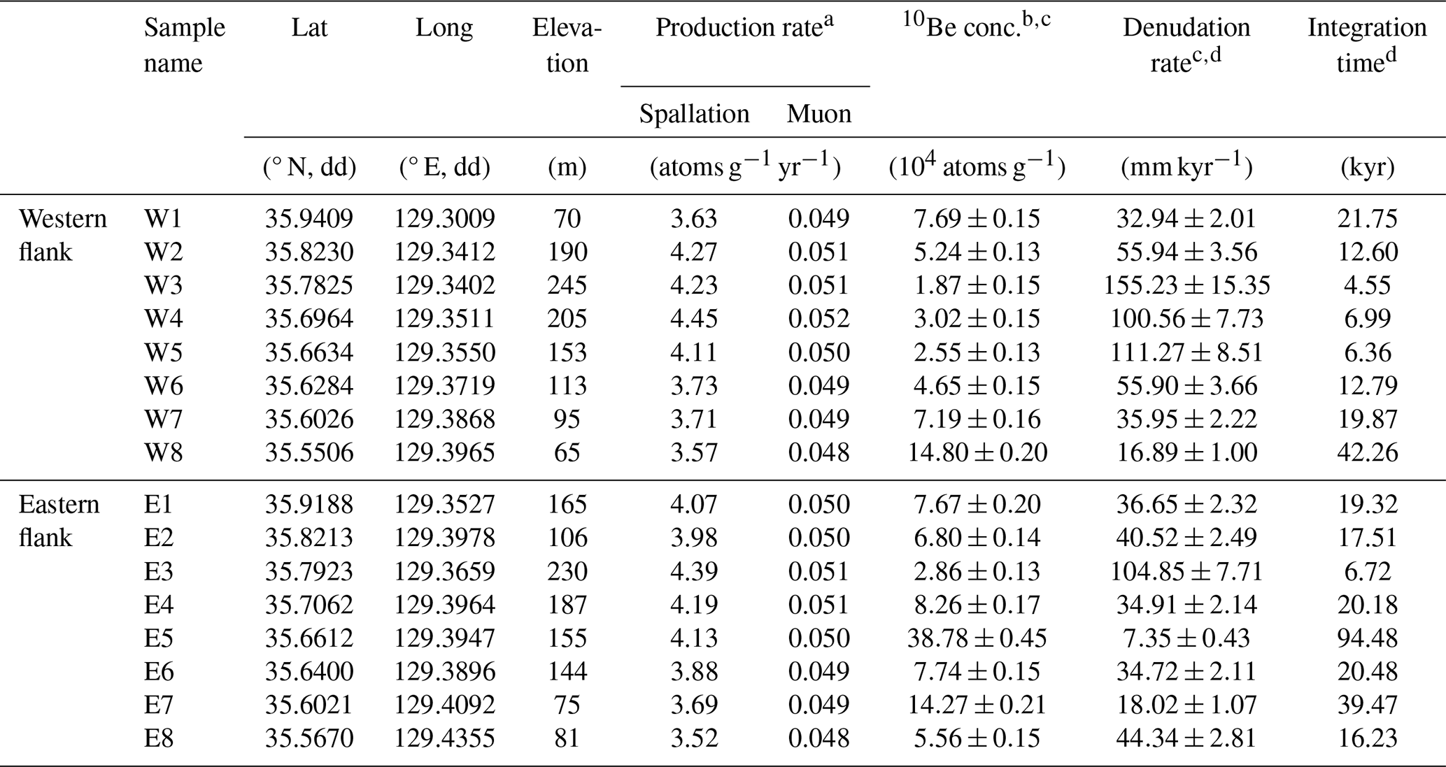
^a Catchment-averaged production rate of in situ ¹⁰Be was computed (Charreau et al., 2019) after applying the LSDn scaling scheme (Lifton et al., 2014). ^b Process blank (4.37–$\mathrm{4.53}\times {\mathrm{10}}^{-\mathrm{15}}$; n=6) was used for correction of the background, and ratios of ¹⁰Be $/$ ⁹Be were normalized with the 07KNSTD reference sample 5-1 ($\mathrm{2.71}\times {\mathrm{10}}^{-\mathrm{11}}\pm \mathrm{4.71}\times {\mathrm{10}}^{-\mathrm{13}}$) of Nishiizumi et al. (2007). ^c Mean values and 1σ uncertainties are used. ^d A ¹⁰Be half-life of 1.38×10⁶ years (Chmeleff et al., 2010), the density of the sample (ρ) of 2.7 g cm⁻³, and an attenuation length (Λ) of 160 g cm⁻² (Braucher et al., 2011) were used to calculate the denudation rate and integration time.

4.2.2 Channel incision rates derived from ¹⁰Be exposure ages of straths

We calculated channel incision rates using in situ ¹⁰Be exposure ages on bedrock straths and using the geometry of the present bedrock channel bed (Table 3). On the western flank, the exposure age of the present channel bed is 2.07±0.12 kyr. The strath is 4.10 m higher than the channel bed, and two samples from the tread yield consistent ¹⁰Be exposure ages of 5.11±0.13 and 4.91±0.13 kyr (mean of 5.01±0.09 kyr) (Fig. 3). Dividing the height of the strath by the age difference between them {4100 mm / [(5.01±0.09) – (2.07±0.12)] kyr} yields a channel incision rate of 1394.56±71.15 mm kyr⁻¹. On the eastern flank, the exposure age of the present channel bed is 12.30±0.15 kyr, and the age of the strath, which is 2.73 m higher than the channel bed, is 24.98±0.20 kyr. The calculated incision rate {2730 mm / [(24.98±0.20) – (12.30±0.12)] kyr)} is 215.30±4.24 mm kyr⁻¹. In summary, at the locations studied, the calculated incision rate on the western flank is approximately 6.5 times higher than that on the eastern flank.

Table 3 Cosmogenic ¹⁰Be surface exposure ages of bedrock strath terraces.

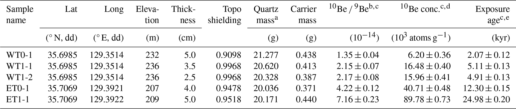
^a A density of rock (ρ) of 2.7 g cm⁻³ was used. ^b Ratios of ¹⁰Be $/$ ⁹Be were normalized with the 07KNSTD reference sample 5-1 ($\mathrm{2.71}\times {\mathrm{10}}^{-\mathrm{11}}\pm \mathrm{4.71}\times {\mathrm{10}}^{-\mathrm{13}}$) (Nishiizumi et al., 2007) and a ¹⁰Be half-life of 1.38×10⁶ years (Chmeleff et al., 2010). ^c Mean values and 1σ uncertainties are used. ^d A process blank (4.37–$\mathrm{4.53}\times {\mathrm{10}}^{-\mathrm{15}}$; n=6) was used for the correction of the background. ^e Ages are calculated assuming zero erosion via the CRONUS-Earth online calculator (version 3.0) (Balco et al., 2008) with scaling factors and applying the LSDn scaling scheme (Lifton et al., 2014).

4.3 Landscape evolution modeling

The MDDs in the initial topographies of Cases A#, which simulated spatially uniform uplift during stage 1, are centrally located within the model domains (Figs. 8a and A1a). In both Cases A1 and A2, after stage 1, the χ indices at the channel heads on the western flank are comparable to those on the eastern flank (Figs. 10a and A1a). However, the MDDs in the initial topographies of Cases B#, which simulated a spatial gradient in uplift rate during stage 1, are biased towards the eastern flank of the modeled domain. After stage 1, the χ indices at the channel heads are lower on the eastern flank than on the western flank in both Cases B1 and B2 (Figs. 9a and A2a). The initial topographies of Cases A# and Cases B# exhibit differences in modeled positions of the MDDs and the patterns of χ indices. These differences are likely due to the variation in the spatial uniformity of uplift rate during stage 1 (uniform vs. non-uniform; Fig. 4b).

4.3.1 Cases A1 and A2

Cases A1 and A2 involved spatially uniform regional uplift during stage 1, followed by spatially variable local uplift related to faulting during stage 2. The modeling results for Cases A1 and A2 show similarities in the drainage configuration (Figs. A1 and 8). During stage 2, the drainage patterns of the initial topographies in both cases undergo minimal change throughout the model domains. The MDDs in both cases remain virtually static, and the channels retain their original routes during stage 2 (Figs. A1a, A1b, 8a, and 8b). The spatial distribution of χ indices in both cases also shows negligible differences compared with the initial topography. In addition, the statistical patterns of topographic metrics for the resultant topographies at the end of stage 2 are almost identical in the two cases (Figs. A1c and 8c). In both cases, the western- and eastern-flank χ indices after stage 2 show no statistical difference (p value >0.05). However, this pattern is inconsistent with the spatial distribution of uplift rate during stage 2. The western flank would show lower χ indices and higher mean upstream relief compared with the eastern flank, as the model simulated a higher uplift rate on the western flank than the eastern flank during stage 2.

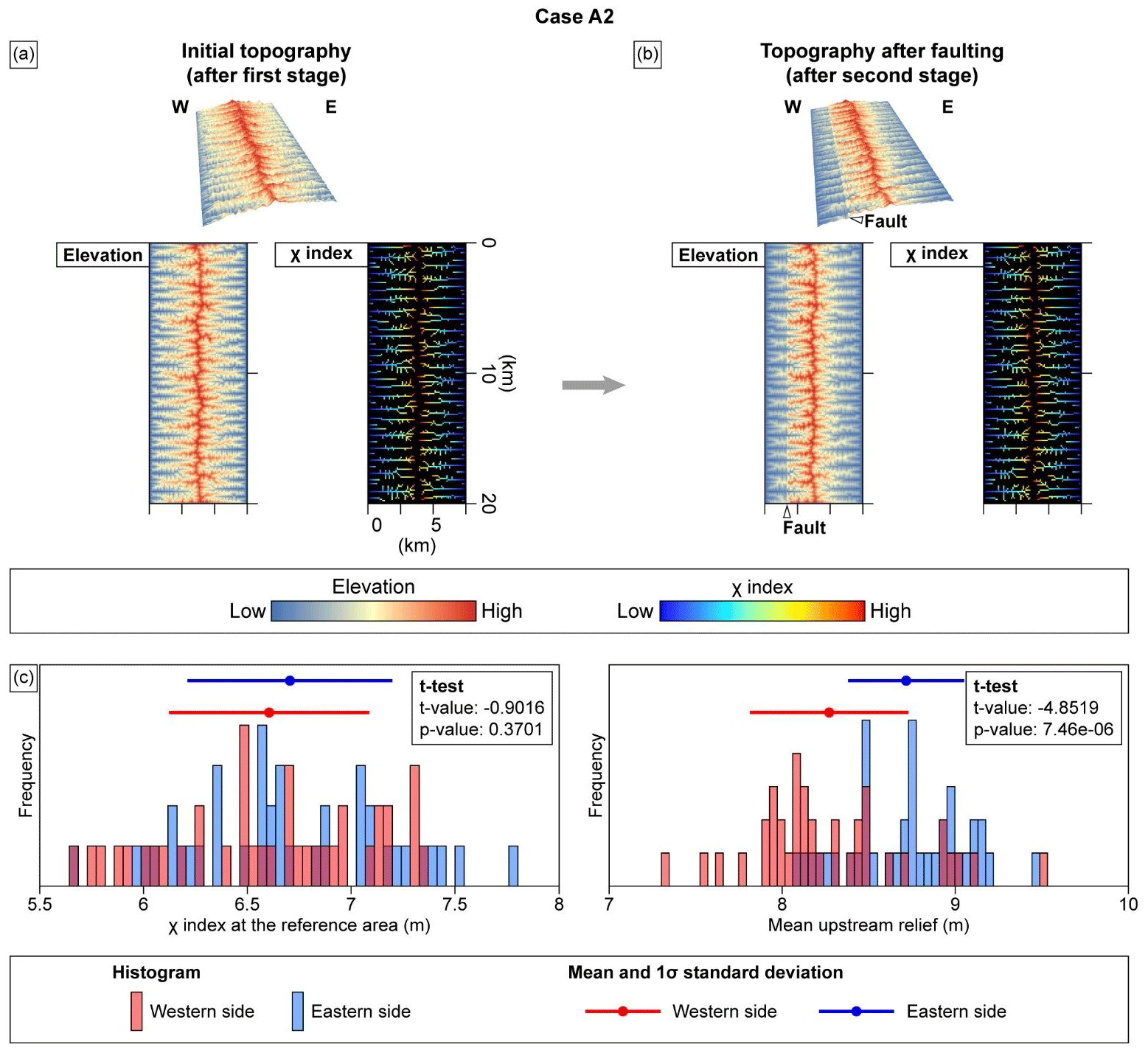
Figure 8 Modeled landscape evolution for Case A2. (a) Inherited topography and χ index after stage 1, simulating a spatially uniform uplift rate of 80 mm kyr⁻¹ over the modeled domain. (b) Topography and χ index after stage 2, simulating fault movement. (c) Histograms, mean values, and 1σ standard deviations for topographic metrics (χ index and mean upstream relief) at the channel heads on the western and eastern flanks of the MDD are extracted from the modeled topography at the end of stage 2.

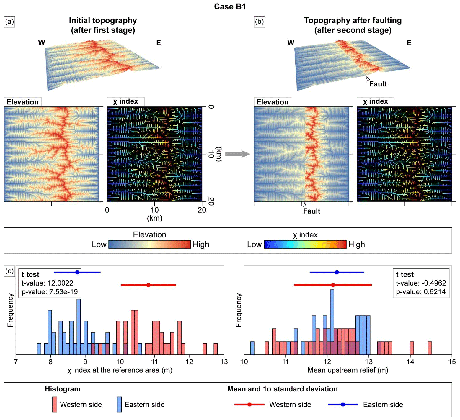
Figure 9 Modeled landscape evolution for Case B1. (a) Inherited topography and χ index after stage 1, simulating a spatially non-uniform uplift rate. The uplift rate is highest at the eastern boundary of the modeled domain (80 mm kyr⁻¹) and decreases with a spatial gradient of −2 mm kyr⁻¹ km⁻¹ towards the west so that the uplift rate is halved (40 mm kyr⁻¹) at the western boundary of the modeled domain. (b) Topography and χ index after stage 2, simulating the fault movement. (c) Histograms, mean values, and 1σ standard deviations for topographic metrics (χ index and mean upstream relief) at channel heads on the western and eastern flanks of the MDD, extracted from the modeled topography at the end of stage 2.

4.3.2 Cases B1 and B2

Cases B1 and B2 involved spatially variable regional uplift during stage 1, followed by the spatially variable local uplift by faulting during stage 2. Case B1 exhibits results similar to those for Case B2 (Figs. 9 and A2). The drainage patterns in these two cases, however, show more noticeable changes during stage 2 when compared with Cases A#. During stage 2, the MDD migrates westwards by 100–800 and 100–1200 m in Cases B1 and B2, respectively (Figs. 9a, 9b, A2a, and A2b). The heightened sensitivity of the MDD to uplift in Case B2 can be attributed to its shorter channels, compared to those in Case B1, allowing the signal of fault activity to propagate more quickly from downstream to upstream. The western-flank channels in both cases shorten during stage 2, losing their upstream areas (Fig. 10b). In addition, the channels undergo subtle changes near the fault. For instance, some channels flowing from north to south or from south to north become shorter or disappear, whereas some new first- or second-order channels that are oriented transversely or obliquely to the fault develop in the vicinity of the fault (Fig. 10b). Despite these key changes in drainage configuration during stage 2, the contrasting χ indices of the western- and eastern-flank channel heads observed in the initial topography persist through stage 2.

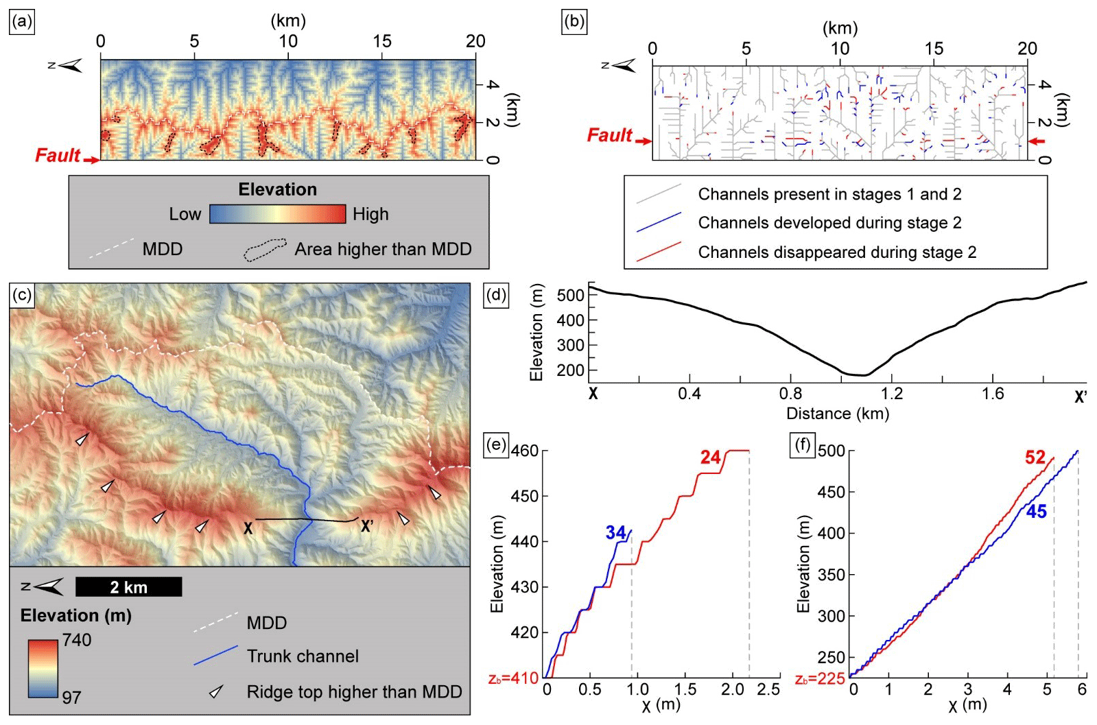
Figure 10 (a) Resultant topography for Case B1, which simulates the northern part of the UFZ study area with asymmetric uplift (westward tilting). Areas with higher elevation than that of the MDD are observed and show similar features to the high ridge top within segment 1 (Fig. 10c). (b) Change in the routes of channels during stage 2 (faulting). The western-flank drainage system loses upstream area, whereas the eastern-flank drainage systems gain upstream area. Some channels parallel to the fault disappear, and new channels oriented oblique or transverse to the fault are developed. (c) The ridge top is higher than the MDD in segment 1. The location of this figure is marked in Fig. 2a. This ridge has elevated, owing to the higher uplift rate on the western flank since the reactivation of the UFZ during the late Quaternary. The antecedent stream flowing within the upstream area in the vicinity of the MDD and the ridge has continued to erode this ridge. (d) Cross-profile of X–X^′ in Fig. 10c. The scale of the horizontal axis and vertical axis of this profile is 1:1. (e, f) χ-transformed profile of the uppermost reach of channels within segments 1 and 2, respectively. These channels are the same as those presented in Fig. 11a and c.

The topography of Case B1 after stage 2 exhibits similar patterns of topographic metrics to those of Case B2 (Figs. 9c and A2c). The eastern-flank χ indices are significantly lower than their western-flank counterparts (p value <0.05). In contrast, the eastern-flank mean upstream relief values are either comparable to (Case B1) or higher than (Case B2) those on the western flank. As with the results for Cases A#, Cases B# also display patterns of topographic metrics that differ from expectations. We expect the western flank to have lower χ indices than the eastern flank in response to higher uplift rate on the western flank during stage 2.

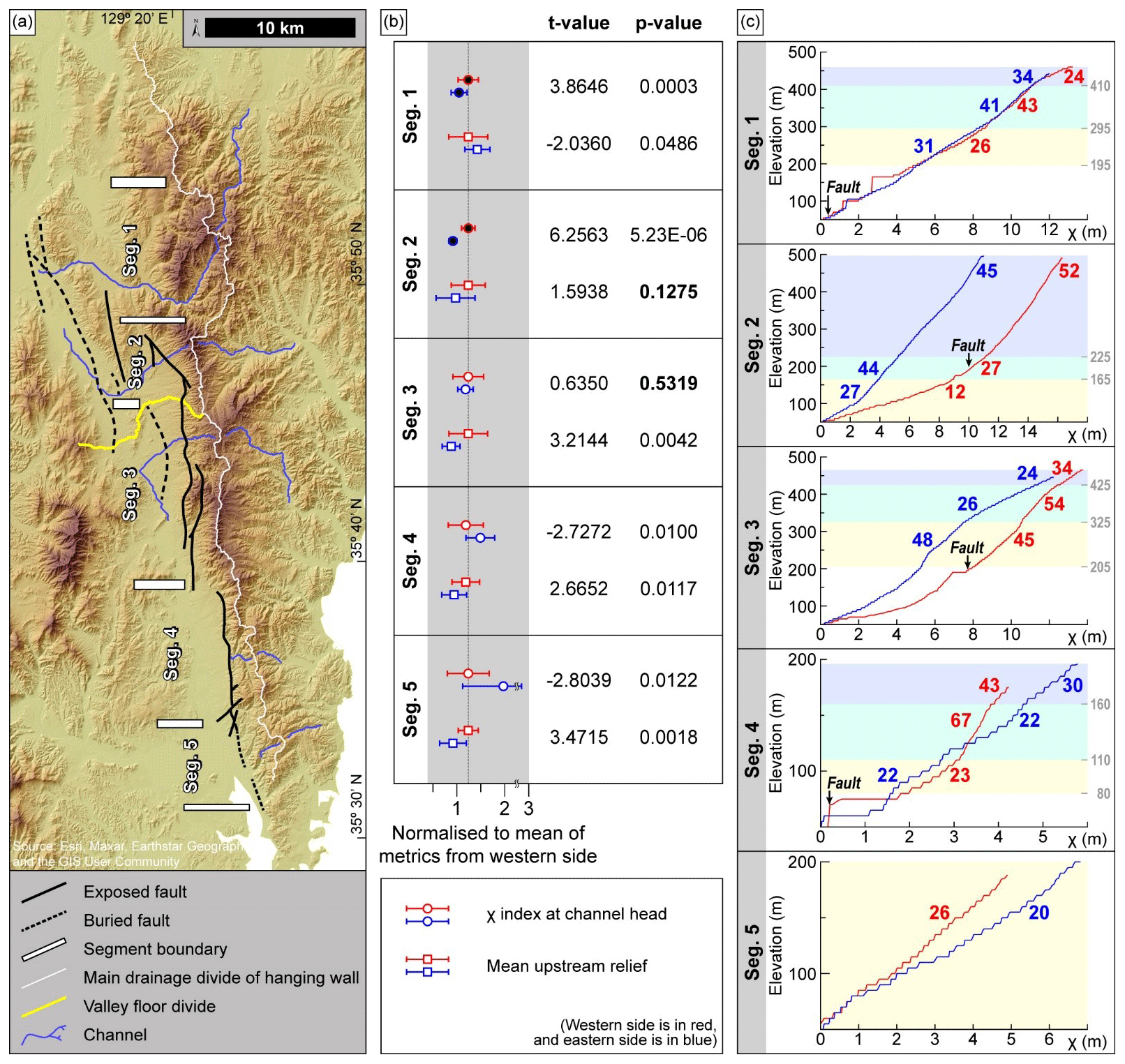
Figure 11 Our proposed segmentation of the UFZ, with corresponding values of topographic metrics presented for each segment. (a) Segmentation of the UFZ proposed in this study. The locations of segment boundaries are the same as those marked in Fig. 7. The segment boundaries are marked with white bars, and the MDD of the TMR is marked with a solid white line. (b) Mean values and 1σ standard deviation of topographic metrics within each segment, normalized to the mean value of each index from the western flank. Topographic metrics on the western flank are in red, and those on the eastern flank are in blue. Symbols filled with black represent decoupled χ indices. We performed Student's t tests to compare these metrics between the western and eastern flanks. P values exceeding the threshold of 0.05 (statistical significance of 95 %) are given in bold, which indicate that the mean values of the western and eastern flank are not statistically significantly different. (c) χ-transformed profiles for one western-flank and one eastern-flank channel from each of the segments shown in Fig. 11a. The numbers represent k_sn of each reach of channel. The profiles for channels on the western flank are plotted with a red line, and those on the eastern flank are plotted with a blue line.

5 Discussion

5.1 Segmentation of the UFZ

Extensive faults or fault zones typically undergo repeated fault patch rupture along specific portions or segments of their lengths. Such faults are called segmented faults with each segment that ruptures during a single seismic event termed an “earthquake segment” (McCalpin, 1996). Identification of fault segmentation is crucial for understanding the geometry, mechanism, and seismological behavior of the neotectonic faults. However, defining the earthquake segment unequivocally can be challenging, unless multiple historical ruptures have been preserved and can be observed, such as that observed in segmented normal fault arrays in low-strain arid settings (Moore and Schultz, 1999). Furthermore, McCalpin (1996) distinguished five different types of fault segments: (1) rupture, (2) behavioral, (3) structural, (4) geological, and (5) geometric segments (Table 9.7 in McCalpin, 1996). The definitions of these segments are listed in order from the most stringent to least restrictive, and the rupture segment is synonymous with the previously defined earthquake segment.

In this study, the UFZ was divided into five geological segments defined using geomorphic indicators and considering fault geometry. Where segments are arranged across step-overs or bends, there may be a zone of cumulative vertical displacement deficit, which is termed a “displacement trough”, in the intersegment zone (Cartwright et al., 1995; Dawers, 1995; Manighetti et al., 2015). We identified displacement troughs on the UFZ by their relatively low tectonic activities on the basis of geomorphic evidence, such as lows in the swath profile, k_sn, relief, and χ index along the MDD (Fig. 7). We reason that relatively low tectonic activity correlates with low values in these topographic metrics, as suggested in other earlier and pioneering studies (Bull, 1977; Cox, 1994; Keller and Pinter, 1996). Areas along the MDD, where the swath profile, k_sn, and relief values are relatively low compared to other stretches, are interpreted as zones of lesser tectonic activity.

Accordingly, we divided the UFZ into five segments (segments 1–5; Figs. 7 and 11). The northern boundary of segment 1 is near the northern tip of the NNW–SSE-striking buried fault. There are lows in the swath profile, mean upstream k_sn, and relief extracted at the base level elevation of 200 m (Fig. 7a and orange lines in Fig. 7b–c). The intersegment zone between our proposed segments 1 and 2 is recognized by the low in the swath profile and the relatively low k_sn extracted at the base level elevation of 200 m (Fig. 7a and orange line in Fig. 7b). The strike of an exposed fault along the mountain front also changes abruptly from NNW–SSE to NW–SE in this intersegment zone (Fig. 11a). Segment 2 has one of the highest swath profiles and high values for several other topographic metrics; the highest observed CADR in the entire study area was also found in this segment (Fig. 7). We divided segment 2 from segment 3 at the point where the next set of lows in the swath profile, k_sn, and relief appear (Fig. 7a and orange lines in Fig. 7b and c). The χ index also has relatively low values at this proposed segment transition (orange lines in Fig. 7d). Furthermore, a NW–SE-striking fault trace terminates between segments 2 and 3, and the strike of the exposed fault changes from NW–SE to N–S there. Additionally, we found a valley floor divide at the intersegment 2–3 zone (Fig. 11a). We demarcated the boundary between segments 3 and 4 at a major fault step-over or jog. The swath profile in this intersegment 3–4 zone shows a marked low (Fig. 7a), and the relief there is also low (both red and orange lines in Fig. 7c). The intersegment zone between segments 4 and 5 is characterized by lows in the both swath profile elevations and k_sn values (Fig. 7a and red lines in Fig. 7b), and relatively low values for the other topographic metrics. The NNW–SSE-striking main fault strand is crosscut by NE–SW-striking secondary faults, and additionally, an exposed fault terminates in our proposed intersegment 4–5 zone.

The longest proposed segment (segment 3) is about 10.25 km long, and the shortest proposed segment (segment 2) is about 4.72 km long (Fig. 11a). Our proposed segment lengths are within the range of surface rupture lengths (SRLs) derived from empirical equations for reverse faults that describe the relationship between earthquake magnitude and SRL (Bonilla et al., 1984; Wells and Coppersmith, 1994). For example, assuming a possible maximum earthquake magnitude of M_W 7.0 (Slemmons and Depolo, 1986; Kyung, 2010), the maximum SRL could be 25.60 km (Bonilla et al., 1984) or 43.58 km (Wells and Coppersmith, 1994). If the SRL is calculated using the magnitude of the Pohang earthquake (M_W 5.4; Fig. 1a), the predicted SRL would be 0.46 km (Bonilla et al., 1984) or 2.13 km (Wells and Coppersmith, 1994). Given these calculations, our proposed geomorphic segmentation lengths seem reasonable, and our proposed segments appear to be physically realistic.

A recent study (Cheon et al., 2023) also divided the incised valley containing the UFZ on the basis of (1) the differences in the fault-hosting rocks and (2) the width of the deformation zone. These authors segmented the UFZ into only two parts, with the division occurring between what we identify as segments 3 and 4 in the current study. We attribute these differences to the different segmentation criteria used and argue that our geomorphic-based fault segmentation has several advantages. First, the use of topographic metrics allows indirect assessments to be made of the relative tectonic activity with spatial continuity over wide study areas. Fault outcrop studies and trench surveys do not have spatial continuity because they provide only point-specific information. Although determining fault segmentation based on observed slip rates would be most accurate, it is impractical due to the large number of geological surveys that would be required to obtain spatially continuous results. Second, geomorphic evidence can be used effectively even in areas where surface deformation is only weakly exposed. It is difficult to identify the direct surface deformation from faulting in Korea because of the low slip rates, rapid physical and chemical erosion, and dense vegetation. However, topography and geomorphology can provide meaningful information on tectonic activity, as the present topography and geomorphology are cumulative results of all past processes.

5.2 Geomorphic evolution of the eastern block of the UFZ in response to tectonic movement

We next used the similarities in the patterns of topographic metrics for fault segment and the modeled topographies to interpret the geomorphic evolution of the mountainous eastern block of the UFZ (Figs. 8, 9, 11, A1c, and A2c). The χ index is suitable for indicating potential future divide mobility, while cross-divide differences in the mean upstream relief are suited to evaluate short-term divide mobility (Forte and Whipple, 2018; Zhou et al., 2022). Although we employed realistic settings for all boundary conditions in the models, based on a comprehensive understanding of the tectonic, geological, and geomorphic processes in the study area, it is acknowledged that there are bound to be significant discrepancies between the modeled and actual values of key variables (e.g., coefficient of erosion, uplift rate, and its spatial gradient), as well as significant epistemic uncertainties.

Since the topography along the MDD varies significantly, each metric (e.g., mean upstream relief or χ index) will encompass a broad spectrum of values. Comparing these means and standard deviations from the western and eastern flanks across the entire MDD might mask genuine differences between the flanks, leading to a “Type II error (false negative: failing to detect a real difference)”. Therefore, we compared each topographic metric from the western and eastern flanks segment by segment.

For segments 2–5, all topographic metrics, except for χ index, generally show a coupled pattern (higher western-flank mean upstream relief and CADR), which indicates higher erosion rates on the western flank (Fig. 9b). In contrast with mean upstream relief and CADRs, the χ anomaly between western and eastern flanks for each segment is inconsistent. The western-flank χ indices in segments 1 and 2 are higher than those of the eastern flank (p value <0.05), the same as those of the eastern flank in segment 3 (p value >0.05), and lower than those of the eastern flank in segments 4 and 5 (p value <0.05). This inconsistency of the χ anomaly throughout the study area is thought to be related to its decoupling from the CADR, channel incision rate, and mean upstream relief in segments 1 and 2. The χ indices in segment 1 are decoupled from the higher CADR and incision rate on the western flank, and those in segment 2 are decoupled from not only CADR and incision rate but also the mean upstream relief. These decoupled χ indices in segments 1 and 2 (i.e., lower χ indices on the eastern flank of TMR) contradict what would be generally expected from the higher CADRs, channel incision rates, and mean upstream relief on the western flank compared with the eastern flank.

To clarify our landscape evolution modeling approach, we grouped our five proposed geological segments into two distinct sections corresponding to the broader northern and southern parts of the UFZ, following but modifying the work of Cheon et al. (2023). Our northern part comprises segments 1 and 2, and our southern part contains segments 3, 4, and 5. Our delineation of the boundary between the northern and southern parts was based on the following criteria: (1) the E–W width of the eastern block of the UFZ at the center of segment 3 is half that of segment 1, (2) the pattern of χ indices shows a noticeable difference at the boundary between the northern and southern parts (i.e., decoupled versus coupled χ indices), (3) the valley floor divide may be a natural boundary between the two parts, and (4) there is an abrupt change in the orientation of faults across this boundary from NNW–SSE to N–S.

5.2.1 Northern part of the UFZ: segments 1 and 2

The geomorphic evolution of the northern part of the UFZ, which is characterized by lower χ indices on its eastern flank, is better explained by Case B1 than Case A1 (Figs. 9c and 11b). χ indices differ markedly between Cases A1 and B1, but the only difference in the boundary conditions between these two models is the spatial uniformity of uplift during stage 1. Case A1 involves spatially uniform uplift, and Case B1 involves spatially variable uplift during stage 1 (Fig. 4). We interpret the lower χ indices on the eastern flank of segments 1 and 2, in comparison to those of the western flank, as a result of the influence of the inherited topography. The northern part of study area may have been in early topographic and geometric disequilibrium (i.e., biased MDD eastwards and asymmetric χ indices). This disequilibrium caused by asymmetric uplift during stage 1 could have persisted to the present day, as simulated in Case B1 (Fig. 9). Topographic and geometric disequilibrium and its persistence by the asymmetric uplift have also been identified in other modeled and natural systems (Willett et al., 2014; Forte and Whipple, 2018; Zhou et al., 2022; Zhou and Tan, 2023). In such cases, disequilibrium caused by the asymmetric uplift persists even after the onset of spatially uniform uplift, until the area reaches equilibrium and the steady state through an adjustment to the uniform uplift (Willett et al., 2014; Forte and Whipple, 2018). In the present study, the northern part of the UFZ has likely remained in disequilibrium as a result of the asymmetric uplift prior to the Quaternary reverse fault reactivation and is still in a transient state that is yet to attain equilibrium even after stage 2.

Within the northern part of the study area, segments 1 and 2 show distinct patterns in the mean upstream relief (Fig. 11). The differences between the two segments can be attributed to two possible factors: (1) the channel length between the fault and the channel head and (2) tectonic activity. Channel lengths between the fault and the channel heads are longer in segment 1 than in segment 2. In segment 1, buried faults are developed in the incised valley, far to the west of the mountain front (Cheon et al., 2023). The response time of a channel to tectonic events increases with increasing channel length between the fault and channel head. Therefore, in segment 1, it is plausible that the most recent tectonic signal from Quaternary reverse fault slip has not yet been transferred to the channel head. Second, the inferred tectonic activity, based on topographic metrics and the CADR (Fig. 7), is higher in segment 2 than that in segment 1. Topographic metrics might be expected to have responded less sensitively to uplift in segment 1 because its tectonic activity is lower than that of segment 2.

5.2.2 Southern part of the UFZ: segments 3, 4, and 5

The pattern of measured χ indices in the southern part of the UFZ is similar to that modeled in Case A2 (Figs. 8c and 11b). Unlike the northern part of the UFZ, the modeled outcome of Case A2 implies that the southern part of the UFZ achieved topographic and geometric equilibrium before stage 2 (Fig. 8a). The lower western-flank χ indices as compared with those for the eastern flank may indicate the adjustment of channels to higher uplift and erosion rates on the western flank after Quaternary reverse fault reactivation on the UFZ. This rapid adjustment to this tectonic perturbation may result from the shorter channel length (between the fault and the channel head) in segments 3–5 compared with those in the northern part of the UFZ. The western-flank χ indices in segments 4 and 5 are lower than the corresponding eastern-flank values. However, there is no difference in the χ index values between the western and eastern flanks in segment 3, which can be attributed to the low base level elevation (z_b) set to calculate the χ index (50 m a.s.l.). This low base level elevation resulted in the integration of a much further downstream reach than the fault location in segment 3, which is less relevant to tectonic uplift (Fig. 11a and c). The upper reaches of the fault have higher k_sn values on the western than the eastern flank, consistent with the pattern of the values of the other topographic metrics, CADRs, and channel incision rates.

Next, we used χ indices from the modeled topography and those observed in the study area to establish the geomorphic evolution of the mountainous eastern block of the UFZ. The northern part of the block underwent spatially variable uplift prior to Quaternary reverse faulting on the UFZ, resulting in the observed asymmetric topography. Conversely, the southern part of the block underwent spatially uniform uplift, attaining topographic and geometric equilibrium prior to Quaternary reverse faulting. Our interpretation on the geomorphic evolution of the eastern block of the UFZ is based on a generalized concept of the influence of pre-existing topography on subsequent geomorphic processes. The pre-existing topography, referred to as “inherited topography”, denotes the topography that existed prior to the event of interest. This inherited topography may include, for example, the channel length governed by the shape of the block and the degree of asymmetry of the topography controlled by the orientations of geological features (e.g., faults) and previous tectonic movements. The four modeling scenarios developed in this study simulated different inherited topographies but for the same early and subsequent tectonic movements. Our model results demonstrate that the geomorphic response to subsequent tectonic movement is influenced by the inherited topography and that topographic metrics (such as the χ index) can be used to measure this influence.

5.3 Migration of the MDD and landscape evolution

Previous assessments of divide mobility have relied on comparing topographic metrics, such as the χ index and Gilbert metrics, of opposing sides of MDD (Gilbert, 1877; Willett et al., 2014; Forte and Whipple, 2018; Kim et al., 2020; Zeng and Tan, 2023). Understanding divide mobility is crucial to the investigating landscape evolution, as it is a dynamic indicator of how the landscape evolves, and it may help determine the driving forces (i.e., tectonic movement and spatial patterns of uplift and erosion) of the evolution. However, we discovered in this study that the χ anomaly may not accurately reflect divide mobility in the UFZ study area because of assumptions involved with determining χ index values. A χ index can correctly indicate the divide mobility only when the area of interest has spatially uniform uplift, climate, lithology, and erodibility (Perron and Royden, 2013; Willett et al., 2014; Forte and Whipple, 2018). The χ-transformed profiles of channels with low base level elevation (z_b=50 m a.s.l.) in segments 2 and 3 show that the uppermost reaches of western-flank channels exhibit higher k_sn and χ index values than the eastern flank (Fig. 11c), giving contradictory results to the expected divide mobility. The higher k_sn on the western flank indicates eastwards divide migration, whereas the higher χ index on the western flank indicates westward divide migration. In this case, instantaneous divide mobility can be accurately evaluated only by comparing the uppermost reaches of channels from opposing sides of the MDD (Zhou et al., 2022). We adopted this approach for the northern part of the UFZ (segments 1 and 2), as the χ indices are decoupled from the CADR, and the bedrock incision rate is there, as well being decoupled from additional topographic metrics used in this study (Figs. 10e, 10f, and 11b).

Uppermost reaches on the western flank in segment 1 exhibit lower k_sn and higher χ index values when compared to those from the corresponding eastern flank (Fig. 10c and e). This suggests that the MDD is migrating westwards in this segment and that it is approaching topographic and geometric equilibrium (see Sect. 5.2.1). Interestingly, we observed that the ridge top of an internal sub-basin on the western flank of the MDD in segment 1 is up to 380 m higher than the MDD itself (Fig. 10c). We propose two possible explanations for this high ridge top: (1) discrete stream capture of western-flank channels owing to the high uplift rate on the western flank and (2) erosion of the ridge top by westward-flowing antecedent streams. The strongest evidence supporting stream capture is the presence of an elbow of capture, wind gap, gorge-like valley, and lower χ index at the channel head of a captor stream (Bishop, 1995; Willett et al., 2014). However, we could not identify any convincing evidence for stream capture, such as an elbow of capture or a gorge-like valley near the ridge top or wind gap near the MDD, in segment 1 in the field or the DEM. In addition, the lower k_sn and higher χ index values of the western-flank uppermost reach in this segment do not imply an aerial gain of the western-flank drainage system owing to stream capture (Fig. 10e). Furthermore, modeling results for Case B1 show similar features of high ridge tops without discrete stream capture. The resultant topography of Case B1, which simulates the landscape evolution of the northern part of the UFZ and spatially variable (asymmetric) uplift prior to late Quaternary reverse faulting, shows some areas with elevations higher than that of the MDD (Fig. 10a). Therefore, we interpret that the streams flowing within the internal sub-basin surrounded by the MDD and the elevated ridge on the western flank (Fig. 10c) are the antecedent streams flowing from east to west. The high elevation of the ridge on the western flank of the MDD is ascribed to the higher uplift rate since the Quaternary reverse faulting of the UFZ. The channels are hypothesized to have been subject to a sufficiently high erosion rate to retain the original stream route of the inherited topography in response to the higher uplift rate on the western flank, but this erosion rate was accordingly insufficiently high to capture parts of the drainage system on the eastern flank.

The western-flank uppermost reach in segment 2 has higher k_sn and lower χ index values than those on the eastern flank, as seen in the χ-transformed profile (Fig. 10f), whereas the profile with lower base level displays a higher χ index on the western flank (Fig. 11c). χ indices at the channel heads are sensitive to base level variations (Forte and Whipple, 2018). In the present case, the lower χ and higher k_sn values of the western-flank uppermost reach indicate short-term migration of the MDD towards the east. This inferred divide mobility is consistent with the results of other topographic metrics such as elevation, mean upstream relief, and mean upstream gradient at the channel head, providing a short-term view of the topographic evolution. Consequently, we interpret that the MDD within segment 2 is migrating eastwards, just like the MDD within segments 3–5, in which patterns of all topographic metrics are consistent with the eastward migration of the MDD.

6 Conclusions

The Ulsan Fault Zone (UFZ) has been one of the most active fault zones on the Korean Peninsula since its reactivation ∼5 Ma. Our study area, the eastern, mountainous, and hanging-wall block of the UFZ, has undergone regional uplift under an ENE–WSW-oriented maximum horizontal stress from 5 Ma to the present (i.e., neotectonics). This study aimed to evaluate relative tectonic activity along the UFZ, characterize the past and present geomorphic processes operating along the UFZ, and infer landscape evolution patterns in response to tectonic perturbation involving reactivation of the UFZ.

We evaluated the relative tectonic activity along the fault zone using topographic metrics, catchment-averaged denudation rates (CADRs), and bedrock incision rates derived using in situ cosmogenic ¹⁰Be. We proposed that the UFZ is segmented into five geomorphic zones based on the relative tectonic activity that we assessed geomorphically. This study represents the first determination of UFZ segmentation based on relative tectonic activity inferred from topographic metrics and, more generally, presents a new method for determining fault segmentation in low-strain, temperate-humid settings.

We also interpreted the tectono-geomorphic evolution of the study area by modeling the landscape evolution and comparing the model values and patterns of topographic metrics with those observed in the study area. We interpret that the northern UFZ (segments 1 and 2) underwent regional asymmetric uplift (westward tilting) prior to Quaternary reverse faulting after ∼2 Ma. The southern UFZ (segments 3–5) was negligibly affected by asymmetric uplift before Quaternary reverse faulting, as the channel lengths (distance between the Ulsan Fault and the channel head) were sufficiently short and able to adjust quickly to stage 2 uplift. Our analysis and interpretation of the tectono-geomorphic evolution of the UFZ show that inherited topography can influence subsequent geomorphic processes and topographic response to neotectonic reverse fault slip. The topographic metrics that we utilized here can therefore be regarded as characterizing not just the present topography but also as holding information resulting from the accumulation of a much longer history of tectonics and erosion.

Our study clearly demonstrates that topographic metrics can effectively be used to infer differential tectonic activity such as variable fault slip and surface uplift. Furthermore, modeling can offer valuable insights into the potential influences of inherited topography in intraplate regions with extremely low strain rates and fault slip rates coupled with high erosion rates.

Appendix A: Results of landscape evolution modeling

Appendix A contains landscape evolution modeling results for the two cases (Cases A1 and B2) that show dissimilar patterns of values of topographic metrics with northern and southern parts of the UFZ.

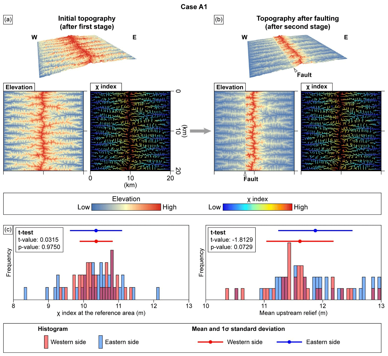
Figure A1 Modeled landscape evolution for Case A1. (a) Inherited topography and χ index after stage 1, simulating a spatially uniform uplift of 80 mm kyr⁻¹ over the modeled domain. (b) Topography and χ index after stage 2, simulating the fault movement. (c) Histograms, mean values, and 1σ standard deviations for topographic metrics (χ index and mean upstream relief) at the channel heads on the western and eastern flanks of the MDD, extracted from the modeled topography at the end of stage 2.

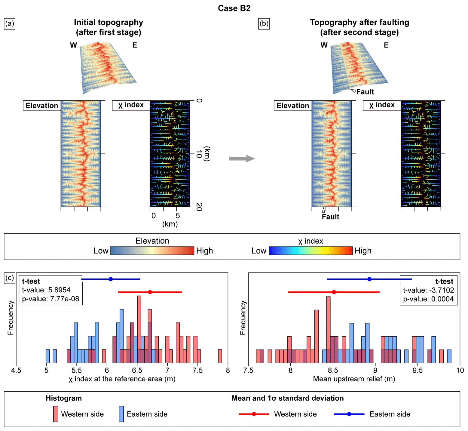
Figure A2 Modeled landscape evolution for Case B2. (a) Inherited topography and χ index after stage 1, simulating a spatially non-uniform uplift. The uplift rate is highest at the eastern boundary of the modeled domain (80 mm kyr⁻¹) and decreases with a spatial gradient of −2 mm kyr⁻¹ km⁻¹ towards the west. (b) Topography and χ index after stage 2, simulating the fault movement. (c) Histograms, mean values, and 1σ standard deviations for topographic metrics (χ index and mean upstream relief) at channel heads on the western and eastern flanks of the MDD, extracted from the modeled topography at the end of stage 2.