the Creative Commons Attribution 4.0 License.
the Creative Commons Attribution 4.0 License.
 | 05 Jan 2024
Introducing standardized field methods for fracture-focused surface process research
Alex Rinehart
Jennifer Aldred
Samantha Berberich
Maxwell P. Dahlquist
Sarah G. Evans
Russell Keanini
Stephen E. Laubach
Faye Moser
Mehdi Morovati
Steven Porson
Monica Rasmussen
Uri Shaanan
Rock fractures are a key contributor to a broad array of Earth surface processes due to their direct control on rock strength as well as rock porosity and permeability. However, to date, there has been no standardization for the quantification of rock fractures in surface process research. In this work, the case is made for standardization within fracture-focused research, and prior work is reviewed to identify various key datasets and methodologies. Then, a suite of standardized methods is presented as a starting “baseline” for fracture-based research in surface process studies. These methods have been shown in pre-existing work from structural geology, geotechnical engineering, and surface process disciplines to comprise best practices for the characterization of fractures in clasts and outcrops. This practical, accessible, and detailed guide can be readily employed across all fracture-focused weathering and geomorphology applications. The wide adoption of a baseline of data collected using the same methods will enable comparison and compilation of datasets among studies globally and will ultimately lead to a better understanding of the links and feedbacks between rock fracture and landscape evolution.
- Article
(8798 KB) - Full-text XML
-
Supplement
(17633 KB) - BibTeX
- EndNote


Rock fracture in surface and near-surface environments plays a key role in virtually all Earth surface processes. Fractures comprise faults and opening-mode fractures, both coming in a wide range of sizes. The focus here, however, is on opening-mode fractures. The propagation of opening-mode fractures universally occurs at or near the surface of Earth (e.g., within ∼500 m – Moon et al., 2020), on other terrestrial bodies (e.g., Molaro et al., 2020), and at depth in the crust (e.g., Laubach et al., 2019). It epitomizes mechanical weathering and the development of “critical zone architecture”, i.e., the evolving porosity, permeability, and strength of near-surface rock (e.g., Riebe et al., 2021). For clarity and consistency herein, the use of the term fracture is limited to refer to any open, high-length-to-aperture-ratio discontinuity in rock, regardless of its origin, scale, or location (e.g., within a clast or within shallow or deep bedrock), acknowledging that veins (partly to completely mineral-filled fractures) or dikes (filled with secondary minerals) are also termed “fractures” in many contexts. The term “crack” is avoided because the wide-ranging semantics of that term can cause confusion when employed in interdisciplinary work across rock mechanics, structural geology, and geomorphology.
Fracture characteristics (e.g., size, number, connectivity, orientation) exert enormous influence on both rock mechanical properties (e.g., Ayatollahi and Akbardoost, 2014) and rock hydrological properties (e.g., Leone et al., 2020; Snowdon et al., 2021). Fractures therefore influence a wide array of natural and anthropogenic landscape features and processes including channel incision (e.g., Shobe et al., 2017), sediment size and production (Sousa, 2010; Sklar et al., 2017), hillslope erosion (e.g., DiBiase et al., 2018; Neely et al., 2019), built environment degradation (e.g., Hatır, 2020), landslide and rockfall hazards (e.g., Collins and Stock, 2016), groundwater and surface water processes (e.g., Maffucci et al., 2015; Wohl, 2008), and vegetation distribution (e.g., Aich and Gross, 2008). Additionally, the resultant physical properties of fracture-produced sediment (i.e., clast size distribution, mass, porosity, etc.) control both hillslope and stream processes (e.g., Chilton and Spotila, 2020; Glade et al., 2019).
With fractures clearly central to so many surface processes, as well as to non-academic concerns such as hazard and infrastructure degradation, it is crucial to understand the factors that control surface and near-surface rock fracture attributes, as well as rock fracturing rates and processes. To fully do so requires a large body of data quantifying fracture-related characteristics and phenomena in a variety of subaerial environments; however, to date, no standard field methods have been widely adopted to quantify fractures in the realm of modern surface processes. Consequently, data collected across studies cannot be readily compared or coalesced. The purpose of this paper is to define an initial set of such standards with the anticipation that the methods will evolve as new understanding, needs, and applications arise. We develop these proposed standards by combining prior fracture methodologies from other geoscience disciplines with those that have been developed, tested, and refined through more than 20 years of field-based fracture observations of surface-process-related research (e.g., Aldred et al., 2015; Eppes and Griffing, 2010; Eppes et al., 2010, 2018; McFadden et al., 2005; Moser, 2017; Shobe et al., 2017; Weiserbs, 2017).
Building on past work, this paper defines the benefits of establishing a standard procedure for fracture-focused surface process field research, describing how presented methods outperform other approaches. We then provide a short review of motivating existing approaches derived primarily from engineering and structural geology disciplines. Finally, we describe a set of methods proposed as a starting point for surface process researchers so that a larger community of teams can begin to cross-pollinate their observations. When no other standard practice is evident in existing literature, we have suggested rules of thumb that are based on our experience during fieldwork for past published works (e.g., Eppes and McFadden, 2010; Aldred et al., 2015; Ortega et al., 2006). We explicitly note when such practices are presented and our rationale thereof. The overall scope herein is limited to in-person field observations on subaerially exposed rock, i.e., fractures that can be observed with the naked eye or basic hand lens. Measurements of smaller fractures (e.g., those visible with microscopy) or of buried fractures (e.g., those visualized in boreholes or with indirect geophysical methods) are not directly described here. We also note that methods for fracture detection using automated analyses of remote data such as lidar, drone photography, structure from motion, or 3D modeling are not described herein but provide motivation for this work (Sect. 1.2).
In sum, the overall aim of this paper is to build (1) a motivation for standardization based on existing published work across disciplines, (2) a set of guiding principles applicable to all surface process research involving rock fractures, (3) a list of fracture and rock data measurements that constitute “basic” field-based metrics, and (4) practical methods that comprise best practices for collection of these data. Unless otherwise specified, all methods may be applied to loose clasts or to outcrops. Also provided are some suggestions for data analyses and a demonstration of a real case example of how the proposed methods lead to reproducible results across users. By providing this compendium of fracture-focused field methods, the hope is to accelerate understanding of how a most basic feature of all rock – its open fractures – contributes to the processes and evolution of Earth's surface and critical zone.
1.1 The value of a standardized approach
Particularly within the fields of geomorphology and weathering sciences, no common suite of data, methods, or terminology has been defined or described that comprises an analysis of fractures. Although fracture characterization field methods exist in the context of structural geology and aquifer and reservoir characterization (e.g., Watkins et al., 2015; Wu and Pollard, 1995; Zeeb et al., 2013; Laubach et al., 2018), they significantly diverge in their approaches because they were largely developed for the specific application of each unique study or field of study. Furthermore, the terminology and methodologies used to describe natural fractures across this existing research tend to be applicable to what is typically envisioned as deep-seated processes including tectonic loading and pore pressure elevation (e.g., Schultz, 2019). Numerous published works fail to provide clear criteria for categorizing fractures or even for choosing which fractures to measure. The choices, of course, depend on the objectives of the study. This lack of consistency severely limits the ability of the geomorphic community to reproduce methods or to combine, compare, or interpret different fracture datasets.
The development of consistent methods undergirds most quantitative Earth sciences. For example, the fields of sedimentology and soil science have clear, standardized methods to acquire what constitutes the basic data for their observations. Sedimentologists have long shared common metrics and methods for quantifying grain size, sorting, rounding, and stratigraphic records (e.g., Krumbein, 1943). Similarly, soil scientists share common methods, metrics, and nomenclature for describing soil profiles and horizons (e.g., Birkeland, 1999, Appendix A; Soil Survey Staff, 1999). The realization of the need for standard methods has also remained constant in laboratory-based rock mechanics over the last several decades, driving the American Society for Testing and Materials (ASTM) and International Society for Rock Mechanics (ISMR) to publish ongoing standards and methods papers (e.g., Ulusay and Hudson, 2007; Ulusay, 2015).
Standards like those mentioned above exist because workers have long recognized and reaped their benefits. Standardized methods can frequently lead to major step-change innovations when data are combined. For example, standardized soil methods allowed for 100 m scale mapping across the United States, enabling detailed human–landscape models that can aid in preserving vital soil resources (Ramcharan et al., 2018). In the field of rock mechanics prior to the 1950s, theoretical developments in rock failure and plasticity lagged other branches of geophysics and engineering. It is likely that progress was limited not only by technology but also, arguably more so, by a lack of consistent methods. Methods for repeatable failure testing were then developed, largely in the groups led by Knoppf, Griggs, and Turner in the United States and Australia (Wenk, 1979). This standardization culminated in the landmark series of papers that comprised the observations driving 50 subsequent years of experimental rock mechanics (e.g., Borg and Handin, 1966; Handin et al., 1963; Handin and Hager, 1957, 1958; Heard, 1963; Mogi, 1967, 1971; Turner et al., 1954).
1.2 Existing fracture measurement approaches across disciplines
For the specific case of fracture-focused research, outside of geomorphology applications, the need for standardized rule-based methods has already been established. Within this prior body of research, engineering and structural geology applications have dominated the development of various approaches.
Engineering geology and geotechnical engineering share common practices in mapping different standards of rock quality and rock mass classification, of which fracture characterization is an important component. The rock quality designation (RQD) was developed in the early 1960s to predict rock mass suitability for building, foundations, tunneling, and other geotechnical issues (Deere, 1964 in Bell, 2007). Within that work, the primary concern is the integrity of the rock, which is governed by its discontinuities, primarily fractures. By providing a standard approach to defining rock quality – albeit qualitative or semi-quantitative – the development of a globally accepted basis of rock mass classification built from RQD and discontinuity surveys has provided a common language for engineering geologists and geotechnical engineers to discuss site suitability and to design critical infrastructure to the point that slope stability parameters, hydrologic suitability, and intact strength can be broadly predicted (Bell, 2007; Hencher, 2015, 2019). Thus, such rock quality metrics may be appropriate for surface process applications, and they provide a rationale and basis for the use of the semi-quantitative methods presented herein.
The rock quality index consists of qualitative classifications from very poor (RQD 0 % to 25 %) to excellent (RQD 90 % to 100 %) based on the linear fracture frequency in core or outcrop line surveys, laboratory velocity measurements, or the ratio of the deformability of the rock mass to that of intact rock (Bell, 2007). Specifically for fractures, rock quality designations are derived only from counts of the number of fractures per foot or core or outcrop. More quantitative estimates of outcrop rock mass quality – commonly used to estimate slope stability quantities – involve measuring multiple lines on an outcrop with estimates of fracture aperture width, hydrologic state (closed, cemented, partially open, open, and flowing), fracture orientation, strength of intact rock estimated with a rock hammer, degree of weathering, and fracture “roughness” or relief along a line of a fixed length, commonly 20 to 30 m (Bell, 2007). These surveys are then repeated periodically with a spacing of ∼100 m, depending on the application (Bell, 2007). Similar methods are used with core and image logging tools (Hencher, 2012, 2015). The fracture parameters are then used in a variety of index models that predict the bulk strength, hydraulic conductivity, and stability of the rock mass. Thus, the extensiveness of the list of measured rock and fracture characteristics in the geotechnical engineering literature reflects the variety of impacts that they have on both each other and the behavior of the rock mass. Here a similar comprehensive list is proposed, but more with surface process applications in mind and thus applicable to a larger range of scale of fractures.
Measurements of the length and aperture of fractures that intersect a line (scanlines), similar to those used for engineering rock quality applications, are widely used and effective in structural geology applications (Marrett et al., 2018; Hooker et al., 2009) and may be valuable where exposures approximate a 1D sample. Selection bias can be avoided by randomly picking scanline directions or by measuring multiple scanlines. To capture all fracture orientations geometric corrections are needed (e.g., Terzaghi, 1965; Wang et al., 2023). When fractures are oblique to scanlines, these corrections are generally more effective if scanlines are long relative to fracture occurrence. Calculations of fracture number density and fracture intensity (Sect. 6.1) require corrections for comparison with 2D data. Depending on the heterogeneity and anisotropy of host rocks, long 1D measures may complicate comparison of fracture patterns to rock properties. Although they are well-suited for capturing the most reproducible and unbiased measure for fracture size, namely fracture aperture distributions (e.g., Marrett et al., 2018) as a 1D measure, without extra measurement steps, scanlines are not well-suited for characterizing representative 2D or 3D rock characteristics or for measuring fracture lengths, heights, or connectivity, all important to surface processes. Thus, in the methods proposed herein, the focus is on 2D “windows”, and an expansion of fracture length measurements – like that proposed by Weiss (2008) – is also detailed so that long fractures are not underrepresented (Sect. 5.4.1).
For 2D characterizations, Zeeb et al. (2013) sought to determine how different sampling approaches lead to censoring bias of different fracture sizes from outcrop data by applying different sampling methods to artificially generated fracture networks that had known parameters. Analysis of data collected using scanline, window, and circular estimator methods revealed that the window approach resulted in the lowest uncertainty for most parameters and required the fewest measurements to provide representative datasets. For areas with large outcrop exposures, circular scanlines combined with a window approach have proven effective (Watkins et al., 2015). Scanlines are also helpful in characterizing simple fracture spatial arrangement attributes. Here, a window approach is outlined that can be employed regardless of outcrop size or fracture number density, both of which could vary considerably in any given surface process field area.
Another consideration that arises in both structural geology and engineering applications is that the methods of fracture (and rock) characterization must include accommodation for rock variations and discipline-specific considerations for specific sites (Hencher, 2015). In particular, the total area(s) of observation and numbers of fractures examined must always be normalized for the specific rock and/or location within the “fracture stratigraphy” of a study (e.g., Shakiba et al., 2023). For example, it is common for sandstone and shaly sandstone to both occur over short distances, and their fracture abundance will vary by rock type (for example, clay-poor sandstones tend to be more brittle and fracture-prone). In this circumstance, the lithologic control on abundance is identified first (this can be qualitative), and then the abundance measures are normalized to the area of the specific rock type. For example, Hooker et al. (2013) employ a reverse procedure, whereby multivariate measures are used to isolate the rock type to which normalization should be confined (if any). A further caution is that all fracture populations in the same rock may not reflect the attributes of the host rock in the same way (all parts of the fracture population may not even be present in all rock types). This variance may arise if fractures are not all the same age because differences in loading paths, exposure histories, and rock properties may vary. Engineering geology applications often map fracture populations in a similar way (Hencher, 2015, 2019) but without the geologic context. Instead, zones are identified and cross-cutting relationships of fractures are commonly used to identify primary vs. secondary planes of weakness. The methods presented herein include instructions for how to make these overall judgments of necessary accommodations and normalizations.
Just as fracture characterization methods must be developed to accommodate variance between and across rock types, they must also be developed so that they are reproducible across users. Above all, it has been established that reproducibility requires clear, rule-based criteria for all decision-making (Forstner and Laubach, 2022). Forstner and Laubach (2022) and Ortega and Marrett (2000) detail issues that arise, particularly from a lack of specificity with respect to identifying features to be measured. In another case example (Andrews et al., 2019), study participants were asked to measure fractures with no particular instructions given for how to collect the data other than where to collect them. The wide variance in resulting datasets collected by different users led to the conclusion that, without common and clearly established measurement and selection criteria, fracture characterization is rife with subjective bias that severely impacts interpretations of results. Then, based on post-data-collection interviews and workshops, Andrews et al. (2019) scrutinized the source of the variance and provided a list of suggested best practices that would serve to best eliminate the subjectivity of data collection that was leading to the bias. In engineering contexts, it is more common to handle such possibility of bias by having fracture mapping during site investigations be performed by a single engineering geologist or by a single small team of trained engineers or geologists (Hencher, 2015). Ideally, either would be carefully reviewed by a senior engineering geology professional. These fracture maps are incorporated into the site model, which is updated – preferably by the same engineering geologist – during construction. In case studies, it is common for poor-quality or inconsistent fracture mapping to lead to incorrectly designed structures, which may fail (Hencher, 2012). Despite these often-dramatic failures, the site-specific nature of fracture networks during rock mass characterization and the balance for a financially successful project may lead to poor review and oversight practices while developing a site model (Hencher, 2015). Here, so that users from different groups may consistently employ this field guide, clear, rule-based criteria are provided that may be used for all measurements described and justify the criteria based on past work and experience.
Including that described above, incorporated in this work are suggested best practices from existing published research on methods. For example, field measurement “crack comparators” are effective for measuring opening displacements, particularly for sub-millimeter widths (e.g., Ortega et al., 2006). Other measurements such as length and connectivity may have low reproducibility (Andrews et al., 2019) owing to various observational and conceptual problems, including dependence on the scale of observation (e.g., Ortega and Marrett, 2000).
In addition to existing field-based fracture research, remote sensing technologies such as lidar, drone photogrammetry, and structure from motion are becoming increasingly common to enable the production of fracture maps whose properties can then be quantified and characterized digitally using freely available software packages such as FracPaQ (Healy et al., 2017). These technologies are rapidly evolving and hold great promise for expanding the scope of fracture measurements overall (e.g., Betlem et al., 2022; Zeng et al., 2023). To date, however, mapping fractures using these techniques holds limitations, such as difficulty distinguishing between fractures and edges, and they are not readily accessible to all field scientists. We believe that it would be premature, and is also beyond the scope of our goals, to try to distill those methods into best practices. Instead, we assert that the methods outlined herein represent a consistent set of methods that could be employed for validation across all such remotely sensed data collection. Furthermore, many of the field methods described herein, such as site and observation area selection, are required for any fracture mapping effort regardless of technique. Thus, many of the methods we present can be applied to most studies using these rapidly evolving remote sensing technologies and should aid in accelerating their development.
Finally, in all cases, the chosen standardized methods presented are optimized for collecting outcrop and clast fracture data relevant to geomorphology and other surface-process-based disciplines (e.g., critical zone sciences, building stone preservation, hydrogeology). The methods described herein are germane to surface and near-surface (<500 m) studies such as validating geophysical measurements, testing factors that influence fracture formation, and documenting links between fracture characteristics and topography or sediment production. Due to a lack of explicit knowledge suggesting otherwise, we present these methods based on an assumption that fractures of all scales (micrometers to kilometers) contribute to all surface processes. Thus, these methods may differ from those of studies with other goals, such as using outcrops as analogs for deep (kilometer scale) subsurface fractures. Such studies aim to distinguish mechanical and fracture stratigraphy, corroborate fracture patterns related to features (i.e., folds or faults), obtain fracture statistics for discrete fracture models (Sect. 1.3), or test efficacy of forward geomechanical fracture models. For these studies applied to understanding deeper deformation, mineral-filled fractures may be more useful or appropriate than focusing solely on open fractures. Also, for deep-Earth applications, near-surface and geomorphology-related fractures are considered “noise” and need to be omitted (e.g., Sanderson, 2016; Ukar et al., 2019). Yet, fractures that are noise to those interested in the deep subsurface are essential features in the context of geomorphology and critical zone sciences. A major outstanding question is how this differentiation might be reasonably and accurately accomplished given the relatively sparse number of studies of fractures in the context of geomorphology. We hope future workers using this guide may find the answers.
1.3 Existing fracture modeling and statistics methods
Once fracture field data are collected, the metrics of their distribution can provide important insights into fracture processes (e.g., Ortega et al., 2006). For example, power-law distributions can be employed as a conservative rule of thumb for determining if enough fractures have been measured (Sect. 4.2). Importantly, however, not all observations of fracture characteristics will be power-law-distributed, with other heavy-tailed distributions possibly indicating other less random controls on fracture properties; this is quite technical, and the reader is referred to Clauset et al (2009). If the dataset is power-law-distributed, however, then the power-law exponent – the slope of the distribution in log–log plots – is the key parameter that determines the distribution of different fracture geometries. While it is tempting to just plot the data on a log–log plot and fit a line, this approach has proven to produce incorrect, strongly biased estimates. Again, without performing correct, unbiased statistical analysis, it is not possible to compare the power-law behavior and other statistics between different carefully and time-intensively collected datasets, limiting how generalizable the results are. The extent to which results may be applicable in surface-process-based fracture studies is an interesting and largely unaddressed question. Thus, for convenience, we outline the details of two straightforward alternative approaches that have been developed for other deeper-Earth applications that surface process workers may utilize with their own data.
To understand fracture length and fracture width data, it is key to first recognize that, with the exception of studies such as in rocks with fractures with uniform spacing and bedding-controlled widths (Ortega et al., 2006), the data can commonly have a heavy-tailed distribution, such as lognormal, gamma, or power law. As mentioned above, of these, strong observational and theoretical evidence suggests that fracture size is commonly power-law-distributed (e.g., Bonnet et al., 2001; Davy et al., 2010; Hooker et al., 2014; Ortega et al., 2006; Zeeb et al., 2013), i.e.,
where b is the fracture dimension (length or width) of interest, n is the number of fractures with dimension b, and A and α are constants. When log-transformed, Eq. (1) becomes
which has led many practitioners to fit Eq. (2) by linearly binning the data in n, then log-transforming the data and fitting the resulting data with a linear regression. This has proven to lead to significant bias in estimates, , of the power-law exponent (Bonnet et al., 2001; Clauset et al., 2009; Hooker et al., 2014) and is not recommended despite its common usage.
Two straightforward approaches have been shown not to have biases or incorrect estimates of the exponent α. (1) The following is based on Clauset et al. (2009). First, the exponent can be found from the cumulative distribution of the dimensions, C(b), or number of fractures with dimension greater than b, i.e.,
where bmax is the maximum size of the fracture dimension (e.g., maximum length or width). The cumulative power-law distribution has the form
It is common to denote 1−α as c. To find α (or c), the dimension data are logarithmically binned. In other words, the dimension data are binned on a logarithmic (1, 10, 100, …) frequency scale and then log-transformed. At this point, linear regression techniques can be applied to estimate α and assess uncertainty. However, in all cases, uncertainty estimates such as R2 will overestimate the certainty for such log-transformed data, but at least the estimate of α is unbiased.
(2) Another method to find α from a dataset of fracture dimensions is to use the maximum likelihood estimator (MLE) given by
where is the estimate of the exponent in Eq. (1), bi is the dimension of the ith fracture, bmin is the minimum valid fracture dimension (see below), and N is the total number of samples (Clauset et al., 2009; Hooker et al., 2014). The MLE estimate has the advantage of an accurate estimate of standard error, σ, given by
Clauset et al. (2009) showed that both the logarithmically binned cumulative distribution and the MLE produce unbiased estimates of the exponent. For all empirical power-law distributions, there is a scale, in this case bmin, below which power-law behavior is not valid. This can be visually assessed by plotting Eq. (2) with logarithmically binned n. The interval between bmin and bmax where the slope is linear is where the power law is valid (Clauset et al., 2009; Ortega et al., 2006), and Clauset et al. (2009) present a formal method to find bmin and bmax. Hooker et al. (2014) use a χ2 test to evaluate the goodness of fit, which is simpler than the p tests of the Kolmogorov–Smirnov statistic proposed by Clauset et al. (2009).
2.1 Natural rock fracturing background
The design of any fracture-related study in the context of surface processes must arise from consideration of the variables that may influence the rates of fracturing and the characteristics of the fractures that form. When rock is proximal to Earth's surface, those variables include factors related to Earth's topography, atmosphere, biosphere, cryosphere, and/or hydrosphere. Here, a very brief overview is provided of some key rock fracture mechanics concepts behind these factors. Eppes and Keanini (2017) and Eppes (2022) provide more detailed reviews of rock fracture and fracturing processes in the context of surface processes.
Rocks fracture at and near Earth's surface in response to the complex sum of all tectonic (e.g., Martel, 2006), topographic (e.g., St. Clair et al., 2015; Moon et al., 2020; Molnar, 2004), biological (e.g., Brantley et al., 2017; Hasenmueller et al., 2017), and environment-related (e.g., Matsuoka and Murton, 2008; Gischig et al., 2011) stresses they experience. Fracturing can occur when stresses exceed the failure criteria (i.e., short-term material strength). More commonly, however, because critical stresses are rarely reached in nature, fractures can also propagate subcritically at stresses as low or lower than 10 % of the rock's strength (see textbooks such as Schultz, 2019; Atkinson, 1987).
Overall, subcritical fracture propagation rates and processes are strongly dependent on stress magnitude, but they are also strongly influenced by the size of the fracture that is under stress (see fracture mechanics textbooks such as Anderson, 2005, or reviews such as Laubach et al., 2019). For single isolated fractures, stresses applied to the rock body are concentrated at fracture tips proportional to the length of the fracture (a concept embodied by the term “stress intensity”), effectively increasing the stresses experienced by that fracture. Simultaneously, as the entire group of fractures within the rock body grows, the rock can become “tougher” – more resistant to further brittle failure under the same magnitudes of stresses, as the total rock mass becomes more compliant (Brantut et al., 2012). Overall, the time dependency of these interacting and contrasting behaviors is not well-characterized in natural settings – deep, shallow, or surface.
In addition to fracture geometry, environmental conditions also strongly impact fracture-tip bond breaking during subcritical fracture. The environmental factors known to impact subcritical rock cracking – separate from their influence on stresses – include vapor pressure, temperature, and pore-water chemistry (Eppes and Keanini, 2017; Eppes et al., 2020; Brantut et al., 2013; Laubach et al., 2019). Therefore, in the context of surface processes, climate matters twice for rock fracturing: (1) as it contributes to the stresses that the rock experiences and (2) as it contributes to the chemo-physical processes that break bonds at fracture tips as they propagate subcritically.
Just as other common physical properties like tensile strength can be measured, rocks can be tested for their propensity to fracture subcritically by the measurement of subcritical cracking parameters such as the subcritical cracking index (e.g., Paris and Erdogan, 1963; Chen et al., 2017; Holder et al., 2001; Nara et al., 2012, 2017). These parameters influence both the rate of subcritical cracking in rock and the fracture characteristics (e.g., amount of fracture per area or fracture length as in Olson, 2004).
In sum, natural rock fracturing is not necessarily the singular catastrophic event that is frequently portrayed in surface process research. Instead, it is likely dominantly a slowly evolving process progressing over geologic time as has been recognized from fracture patterns in bedrock (e.g., Engelder, 2004; Rysak et al., 2022) and more recently in the context of surface processes (Shaanan et al., 2023). Importantly, however, there are currently few field-based data elucidating these complex, experimentally observed phenomena in surface process contexts. It is therefore our hope that this guide will enable more workers to document the complex feedbacks between rock and fracture properties, as well as environmental, topographic, and tectonic factors, that likely influence all fracturing at and near Earth's surface.
2.2 Study design and site selection using a state factor approach
Due to their influence on rock fracturing as described above, all potential driving stresses and variations in fracture environments must be considered in study design and site selection for any fracture-related research. Parent rock, topography (and other loads), climate, biota, and time all potentially impact initiation and propagation of surficial fractures in rocks. Though this idea might generally exist in other fracture-focused research, in the field of soil geomorphology it has long been explicitly described as a “state factor” approach (e.g., Jenny, 1941; Phillips, 1989) to understanding progressive chemical and physical alteration processes. Thus, we propose that this well-vetted conceptual paradigm may be employed in fracture-focused surface process research as a standard.
Here, it is asserted that applying a state factor approach to fracture research is relevant because fracturing processes are influenced by each of these factors, like all other chemical processes acting on rock and soil. This is particularly true when the subcritical nature of rock fracture is considered (Sect. 2.1). Thus, all state factors that could contribute to fracture propagation styles and rates should be explicitly considered and controlled for as much as possible within the aims and scope of the research for any given site. These state factors – long categorized as they relate to overall soil development, of which physical weathering is a component (e.g., Jenny, 1941) – are equally applicable to fractures alone and include climate (cl, both regional climate and microclimate), organisms (o, flora and fauna), relief (r, topography at all scales), parent material (p, rock properties), and time (t, exposure age or exhumation rate). For rock fracture, tectonics (T) should be added to this list, making cl, o, r, p, t, and T.
Hereafter, the term “site” refers to a single location of either a group of rock clasts or a group of outcrops, whereby all clasts or outcrops within the site could be reasonably assumed to have experienced similar state factors over their exposure history. For example, a site might comprise a single boulder bar on an alluvial fan surface or a single ridgeline with several outcrops. Once the specific state factors (including the internal variability of each site) are identified for all the sites within a given field area, a series of sites can be selected whose state factors are known and controlled for as much as possible. This enables a study of the influence of individual factors across the sites, i.e., fracture chronosequences, climosequences, toposequences, or lithosequences.
For rock fracture, it is important to understand how each cl, o, r, p, t, and T factor may contribute to stresses that give rise to fracturing and/or to the molecular-scale processes that serve to subcritically break bonds at fracture tips (Sect. 2.1). Based on existing experimental data and weathering research, and without evidence to show otherwise, we infer that each has the potential to independently impact fracturing rates, styles, and processes in surface process contexts. The following descriptions provide only brief examples from the literature as to how each of the state factors may influence rock fracture. To fully describe each of their influences on rock fracturing in general would comprise a textbook. Assuredly, to date, there are insufficient data to propose a hierarchy of their influence on fracture characteristics in surface process contexts. The factors are therefore listed in the cl, o, r, p, t, and T order by traditional convention only.
2.2.1 Climate (cl)
Climate (cl) as a state factor refers not just to regional mean annual precipitation or temperature, but also the local microclimate of a site, which may be influenced by site characteristics, such as runoff or aspect. The presence of liquid water increases the efficacy of water-related stress-loading processes like those related to freezing (Girard et al., 2013) or chemical precipitation of salts or oxides (e.g., Buss et al., 2008; Ponti et al., 2021). Moisture – particularly vapor pressure – can also serve to accelerate rock fracturing rates independent of any stress loading (e.g., Eppes et al., 2020; Nara et al., 2017). Temperature cycling can produce thermal stresses (through differential expansion and contraction of both adjacent minerals as well as different portions of the rock mass, e.g., Ravaji et al., 2019), and can also influence rates and processes of fracture-tip bond breaking (e.g., Dove, 1995).
2.2.2 Organisms (o)
Organisms (o) refer to both flora and fauna – everything from overlying vegetation and large animals to roots and microorganisms, all of which may provide a source of rock stress and/or may influence water availability or chemistry. These relationships can be complex and unexpected. For example, tree motion during wind and root swelling during water uptake both exert stresses on rock directly (Marshall et al., 2021a). Organism density and type can impact rock water and air chemistry (Burghelea et al., 2015), both of which may impact the rates and processes of subcritical cracking (e.g., review in Brantut et al., 2013).
2.2.3 Relief (r)
In the context of state factors, relief (r) generically refers to all metrics related to topography including aspect, slope, and convexity. Topography impacts the manifestation of both gravitational stresses and tectonic stresses within the rock body (Molnar, 2004; Moon et al., 2020; Martel, 2006). The directional aspect of a particular outcrop or boulder face may also influence insolation and water retention, translating into differences in microclimate and vegetation and, thus, weathering overall (e.g., Burnett et al., 2008; West et al., 2014; Mcauliffe et al., 2022), including fracturing (e.g., West et al., 2014).
2.2.4 Parent material (p)
The parent material (p) factor in the context of a fracture study refers to the specific rock type(s) containing fractures (and potentially undergoing fracture) in the geomorphic environment. Rock varies in the types and dimensions of material present (e.g., sandstone, siltstone, shale, basalt, granite) and the types and spatial arrangements of interfaces within the material (e.g., grain size, porosity, bedding, foliation). These properties directly influence the rates and styles of fracture propagation (Atkinson, 1987) due to how they respond to stresses but also due to how they allow stresses to arise (e.g., through their compliance, thermal conductivity). Thus, different rock properties differently influence the rates and characteristics of fracture growth and susceptibility to topographic and environmental stresses. For example, different minerals are characterized by different coefficients of thermal expansion. As a result, rocks with different mineral constituents will be more or less sensitive to thermal stresses than others depending on the contrasts between adjacent grains. Rock mineralogy will also impact chemical processes acting at fracture tips during subcritical cracking, as well as the overall susceptibility of the rock to chemical weathering.
Many (perhaps most) rocks contain fractures that formed prior to exposure, either due to deep-seated tectonics and fluid pressure loads or to thermal and mechanical effects due to uplift towards the surface (English and Laubach, 2017; Engelder, 1993). In sedimentary rocks, fracture patterns (and, in some cases, fracture stratigraphy) vary with mechanical stratigraphy (e.g., Laubach et al., 2009) that can also influence near-surface fracture. In many instances, mechanical properties may be reflected in fracture stratigraphy, and vice versa. Schmidt hammer measurements are a useful, fast, and inexpensive field approach to documenting mechanical property variability (Aydin and Basu, 2005); however, such measurements are impacted by weathering exposure age (e.g., Matthews and Winkler, 2022). The influence of fracture characteristics of the parent rock that may have formed in the deep subsurface is described in Sect. 2.2.6 (Tectonics).
Additionally, in the context of surface process studies, we propose that parent material also refers to the size and shape of the clast or outcrop because, for example, angular corners generally concentrate stresses more than rounded edges (Anderson, 2005). Also, clasts or outcrops of different sizes experience different magnitudes of thermal stresses related to diurnal heating and cooling (Molaro et al., 2017).
2.2.5 Time (t)
Time (t) likely plays a role in rock fracturing rates just as it does in chemical weathering, whereby outcrops found in slowly eroding environments or clasts on old surfaces may be subject to different fracturing rates and processes (e.g., Mushkin et al., 2014). Over time, rock mechanical properties can also change as weathering occurs (e.g., Cuccuru et al., 2012). Although the time factor has not been well-studied in the context of natural rock fracture, preliminary data suggest that it should be considered (Berberich, 2020; Rasmussen et al., 2021). Published surficial geologic maps or datasets of rock exposure ages or erosion rates (e.g., Balco, 2020) can provide “time” information for rock surfaces, and the subaerial opening of fractures themselves can be dated using luminescence techniques (Andričević et al., 2023).
2.2.6 Tectonics (T)
Finally, in a fracture-related study, the tectonic (T) setting must also be considered a state factor. Fractures that have formed in the deep to near subsurface in response to tectonic forces such as plate-scale stress fields, folding, and faulting (and attendant pore pressure variations) may continue to propagate at or near the surface, and they inevitably become exhumed. Overall, fractures formed by these processes have traditionally been studied within the structural geology discipline, and that literature is extensive (e.g., reviews in Laubach et al., 2018, 2019; Atkinson, 1987, Chapter 2). The tectonic history of rock can be recorded or manifest in its brittle structures that are then maintained over a wide range of past tectonic events, including its most recent exhumation and cooling. The attributes of resulting open or filled fractures depend on how deeply the material was buried and how rapidly uplifted, as well as the material properties (e.g., English and Laubach, 2017). Finally, the fact that the current tectonic setting can drive ongoing deformation has long been recognized (e.g., Hooke, 1972), and more recent work has highlighted that very low-magnitude tectonic stresses can translate to fracture propagation in very near-surface bedrock, especially when interacting with local topography (e.g., Martel, 2011; Moon et al., 2020).
It is likely, though perhaps not widely appreciated, however, that fractures originally opened due to tectonic stresses further propagate, not only due to ongoing tectonic stresses as they approach the surface, but also due to topographic and environmental stresses that the rocks increasingly encounter as they are exhumed to shallower depths. Simultaneously, these “new” stresses may increase the overall number density (total number of fractures per area) and fracture intensity (defined here as total fracture length per area). These changes in fracture characteristics may manifest abruptly with depth or more gradually, and those changes may manifest differently under different topographic portions of the landscape (e.g., ridges versus valleys). There is a growing body of data pointing to such surface interactions (e.g., Marshall et al., 2021b; Moon et al., 2019, 2020; St. Clair et al., 2015), but overall, these differentiations are a topic ripe for further study.
Pre-existing fractures may not always be easily separable from those formed or further propagated under geomorphological influence. Environmental stresses also produce parallel fractures (e.g., Aldred et al., 2015; Eppes et al., 2010; McFadden et al., 2005), as do those related to the morphology of the eroding landscape (Leith et al., 2014). Thus, for outcrops, and particularly for clasts where correlations or comparisons with regional tectonic structures are not possible, fracture orientations may not uniquely represent a tectonic regime. The non-geomorphic origin (or otherwise) of such fractures may be evident from microstructure analyses that examine fractures for diagenetic cements, inconspicuous mineral deposits, fluid inclusions, or other similar features (e.g., Ukar et al., 2019). Thus, in choosing study sites, consideration should be made of rock age, tectonic history, and current tectonic setting (e.g., World Stress Map, Heidbach et al., 2018), as well as unambiguously tectonically related structures such as dipping bedding planes, evidence of mineral deposits in the fractures, stylolites, or ductile structures such as folds (Hancock, 1985; Laubach et al., 2019).
2.3 Bedrock outcrops versus deposited clasts
The fracture characteristics of outcrops have long been employed as proxies for subsurface fracture networks, and there is a reasonably large body of literature addressing these relationships and their potential pitfalls (e.g., Ukar et al., 2019; Al-Fahmi et al., 2020; Sharifigaliuk et al., 2021). However, based on the growing body of research mentioned above, topographic and environmental stresses have both likely contributed to any subaerially observed fracture network unless otherwise ruled out. Thus, for studies that aim to isolate fractures associated with environmental stresses, measurements from clasts may be more useful than outcrops.
Clasts that have been transported by fluvial, glacial, or mass-wasting processes have experienced abrasion, and therefore it is highly likely that pre-existing superficial fractures have been removed. Thus, clasts may be more reasonably considered “fresh” than an outcrop with an unknown exhumation history, allowing clearer linkages between environmental exposure and observed fractures. This idea of “resetting” fractures within clasts through transport is supported by data showing that clasts of identical rock type that have experienced more transport (i.e., rounded river rocks) have higher strength than those found in, for example, recent talus slopes (Olsen et al., 2020). Nevertheless, clasts may carry with them an invisible (to the unaided eye) population of pre-existing fractures – or sealed microfractures – that in some instances impart a strength anisotropy that can manifest in later surface-related fractures, even in clasts. Thus, for such rocks, the reset may be imperfect (e.g., Anders et al., 2014). In-depth petrographic analysis to identify residual microstructures (e.g., Forstner and Laubach, 2022) may not be feasible in most instances, but a simple uniaxial point load tests, or field Schmidt-hammering of clasts found in active channels, may reveal whether an inherited anisotropy is present.
Carefully selecting the rock surface area(s) on which fractures will be observed and measured within a site is equally as important as selecting the site or the fractures themselves. Hereafter, the term “observation area” refers to the specific portion(s) of rock surface(s) for which fractures are being measured. Observation areas may comprise the entire exposed surface of individual clasts, outcrops, or portions of either (Fig. 1). In the following sections, instructions for selecting these observation areas in the field are provided.
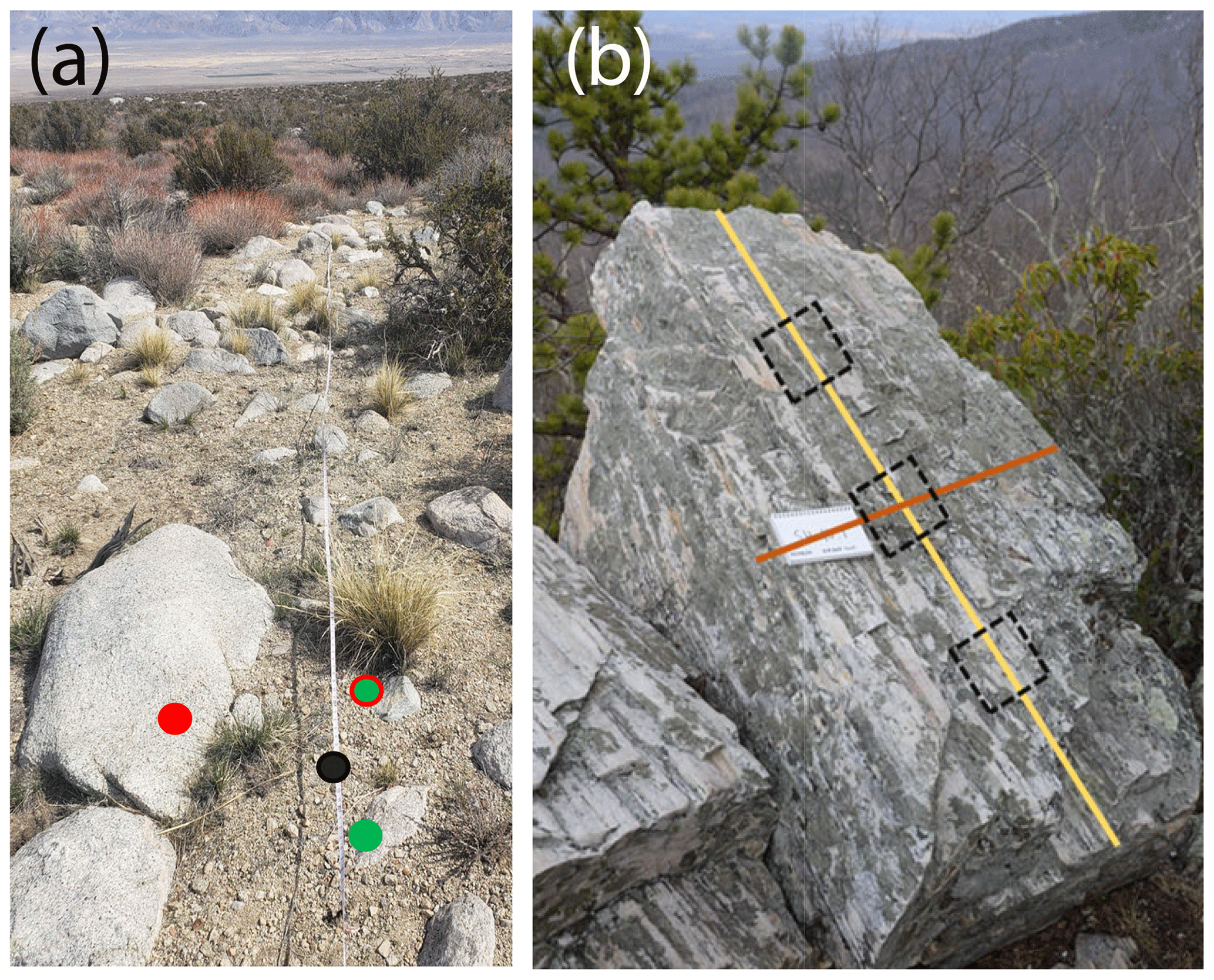
Figure 1Images illustrating the selection of observation areas for clasts and outcrops. (a) Photograph of a transect established for clast selection. Black dot: predefined transect interval location on the tape. Red dot: clast that does not fit the predefined clast selection criteria (e.g., it is too big). Green dot with red circle: clast that fits criteria but is further away from the interval point than the clast with the green dot. Green dot: closest clast to the transect interval that meets the selection criteria. (b) Annotated photograph showing an idealized placement of “windows” (dashed black squares) on a bedrock outcrop. Outcrop dimensions are measured and the windows are placed using predetermined selection criteria. In this example, the windows are equally spaced along the centerline of the long dimension of the upward-facing side of the outcrop.
3.1 Establishing outcrop or clast selection criteria
Before observation areas can be identified, outcrops or clasts must be selected. The first step of that selection process is to establish criteria for determining which outcrops or surface clasts within the site are acceptable for measurement. Without evidence to proceed otherwise, similar to site selection, variability in cl, o, r, p, t, and T factors that may influence fracturing (e.g., temperature, moisture availability, rock shape, and rock type) should be controlled for as much as possible.
In general, characteristics of the clasts or outcrops that might impact mechanical properties, moisture, or thermal stress loading should be most heavily considered. The rock type properties that should be considered when developing selection criteria include not only heterogeneities like bedding or foliation, but also grain size and mineralogy, all of which can influence fracture rates and style characteristics. For example, perhaps only outcrops with no visible veins or dikes will be employed, only outcrops greater than 1 m in height, or only north-facing outcrop faces. Past work, for example, has focused on upward-facing surfaces of outcrops or large clasts (e.g., Berberich, 2020; Eppes et al., 2018).
For loose clasts, only clasts of a particular size or rock type might be employed for measurement. For example, past work found that below approximately 5 cm diameter in semi-arid and arid environments (Eppes et al., 2010), and 15 cm in more temperate environments with vegetation (Aldred et al., 2015), clasts are more likely to have been moved or disturbed. Thus, these sizes were employed as a threshold for selection.
3.2 Non-biased selection of clasts or outcrops for measurement
Once criteria are defined, clasts or outcrops meeting those criteria must be randomly chosen for the fracture measurements. A procedure similar to the well-vetted Wolman pebble-count-style transect (Wolman, 1954) should be employed to avoid sampling bias. For landforms with other geometries, a grid may be used instead of a transect line.
In either case, a tape transect or net grid is laid out on the ground at each site, and the clast or outcrop closest to specified intervals on the tape (or at the points of the grid meeting the criteria) is selected (Fig. 1a). The interval or grid spacing should be adjusted to the overall size and abundance of clasts or outcrops found on the surface. If there are relatively few meeting the criteria at a site, all within the site meeting the criteria can be measured.
A similar technique can and should be applied for selecting outcrops. For example, care should be taken not to be limited to the “best” outcrops (cleanest and/or largest), since they are likely the least fractured. However, such large, clean outcrops may be the best places to observe any pre-existing subsurface-related fractures. For locations where outcrops are within a few meters or tens of meters of each other and vegetation is relatively sparse, a grid of a set dimension (e.g., 100 m) is overlain on aerial imagery, and the closest outcrops to each grid intersection meeting the outcrop criteria are selected (Watkins et al., 2015). For areas where outcrops are not visible in aerial imagery, a measured or paced transect can be employed where the user walks along a bearing and chooses the closest outcrop meeting the selection criteria at each interval, e.g., 30 paces.
In all of the above, transect locations and orientations should be selected following consistent criteria and being mindful of the state factors cl, o, r, p, t, and T. For example, all transects or grids might be placed uniformly along backslopes with a certain upslope distance from the crest or along the latitudinal center or crest of a landform. Alternatively, the transect might be oriented perpendicular or oblique to a paleo-flow direction so that it is not constrained only to bars or swales. The coordinates and bearing of all transects or grids should be recorded, enabling tracking and avoiding repetition.
3.3 Observation areas comprising the entire clast or outcrop surface
Fractures are three-dimensional objects, and ideally observations should encompass volumes; but, this is precluded by the opacity of rock, so one- or two-dimensional observation areas must be used. Fracture arrays may also encompass a wide range of sizes, so the selection of observation area(s) needs to consider truncation and censoring biases.
The observation area for small clasts and outcrops can be their entire exposed surface. In our experience, when clasts or outcrops selected for measurements are less than ∼50 cm in maximum dimension, measurements can typically be readily made for all fractures visible on the clast or outcrop exposed surface for most rock types.
We strongly suggest that rocks not be moved during measurement. This non-disturbance practice is particularly crucial for maintaining Earth's geodiversity (Brilha et al., 2018) and preserving sites for future workers to revisit. Further, research examining acoustic emission localization of rocks naturally fracturing found that the large majority of fracture “foci” were located in the upper hemispheres of boulders (Eppes et al., 2016). Thus, we infer that the potential insight gained by moving clasts does not warrant the impact on geoheritage.
3.4 Establishing windows as the observation area for larger clasts and outcrops
Particularly for larger exposures, it is not feasible to measure every fracture on an outcrop or clast. In these cases, the observation area may comprise predetermined windows of representative decimeter- to meter-scale areas of the rock surface (Fig. 1b). This window selection method results in an accurate representation of fractures on an entire outcrop (e.g., Zeeb et al., 2013) and is least affected by subjective biases (Andrews et al., 2019).
Importantly, the number and size of windows observed on each outcrop or at each site should depend on the typical number and size of fractures present on the surface of the rock (Sect. 4.2). Inevitably it is our experience that logistical constraints will dictate that decisions must be made about size cutoffs. Some part of the smallest size fraction of fractures may not be readily visible, and the finite size of exposures may mean that some large fractures are missed. Overall, it is preferable to strike a balance between window size and number so that during data analysis, variance can be quantified by comparing data collected between windows on the same outcrops and at the same site. More total observation area (e.g., more and/or larger windows) is required when fractures are fewer per area. The size of the area required for a representative quantification of fractures depends on both fracture average length and number density (e.g., Zhang, 2016). Here, an iterative approach is outlined for determining if sufficient area has been examined (Sect. 4.2), but other rules of thumb exist, particularly in the rock quality designation index literature (e.g., Zhang, 2016).
Choosing the placement of windows on the outcrop should entail a stratified random sampling approach. Just as for clast or outcrop selection, cl, o, r, p, t, and T factors like aspect should be taken into consideration and controlled for as much as possible in the window placement strategy by, for example, only using upward-facing surfaces. Then, window placement determination is made to avoid sampling bias and edge effects. For example, if upward-facing outcrop surfaces are to be characterized, then the total length and width of the face could be employed to align sufficient numbers of windows along even intervals of those measurements (e.g., three windows whose centers are located along the center axis of the rock with even spacing between the edges and each box; Fig. 1b).
For the placement of each window, it is our experience that a simple cardboard template of the appropriate window size with a center hole can be employed to trace the window with chalk directly on the clast or outcrop. Then, all fracture measurements are made in the window(s). Each window should be numbered and photographed in the context of each outcrop or clast. Also recommended is detailed photo-documentation of each outcrop and transect, along with sufficiently detailed coordinates to reoccupy the precise site (e.g., in meters or 0.00000 decimal degrees that are always referenced to the projection or datum used).
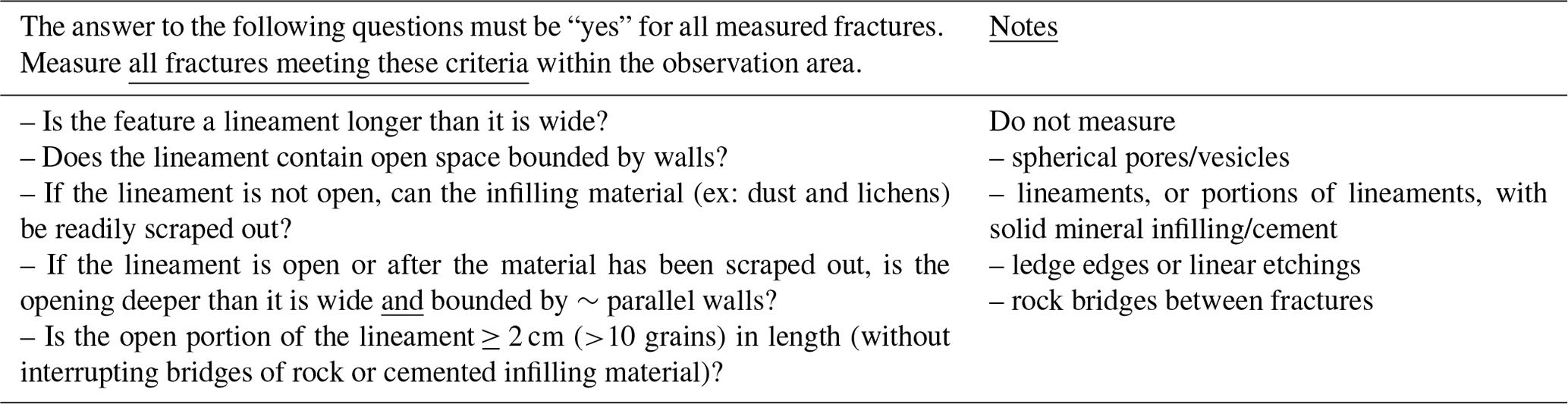
Table 1List of proposed rule-based criteria for defining measurable fractures.
3.5 How many observation areas?
The number of clasts, outcrops, or windows required to measure sufficient fractures will vary with the study goals, site complexity, and the variables for which the data are being tested or controlled. Importantly, for each study, the required number of observation areas must be established based on the amount of area necessary to gain a statistically sufficient number of fracture observations to represent the rocks in question for that setting (Sect. 4.2). Concepts of “stationarity” have been applied in the context of 2D analyses (e.g., Shakiba et al., 2023), but no rule of thumb in the context of surface processes is described herein because, as yet, there have not been sufficient standard fracture data collected to establish such a rule. Establishing such a rule of thumb is an illustration of the motivation of this paper, as well as an example of how the methods presented herein can and should evolve over time.
Rocks or outcrops with lower fracture number density (fewer overall fractures per area) will require larger areas of their surface to be examined to measure sufficient fractures for statistical significance (Sects. 3.4 and 4.2). Rocks or outcrops with significant variation in fracture patterns require sufficient observation to capture that variability. Thus, as an example only, in past work, when state factors were carefully controlled for, relationships between rock material properties and rock fracture properties were evident from about 3 to 5 m scale outcrops per rock type on ridge-forming quartz-rich rocks (Eppes et al., 2018). However, until a sufficient magnitude of datasets has been collected for a particular site, the amount of observation area must be established based on the number of fractures uniquely available at each study site.
4.1 Rule-based criteria for selecting fractures in surface process research
The term “fracture” is employed with a wide variety of meanings across the geosciences, potentially resulting in large variations in the range of features that two individuals might study on a single outcrop (Long et al., 2019). Therefore, it is crucial to employ clear and repeatable rule-based criteria (e.g., Table 1) for what constitute measurable fractures within any fracture-related research. Failing to do so consistently results in a high variance of subjective bias that is more reflective of worker personality than of the variance in fracture of the outcrop (Andrews et al., 2019). Thus, consistency and documentation are required for deriving interpretable and repeatable results.
The proposed rules (Table 1) for determining which fractures to measure at any given field site were developed by us in the context of surface process research and through iterations with numerous non-expert users (undergraduate students) to arrive at criteria that provided consistency in observations across users. Because surface processes are frequently and largely dependent both on rock erodibility and water within a rock body, the recommended criteria are applicable only to open voids, which are known to greatly impact both. Also, because other types of open voids like vesicles are common in rock, an additional criterion is that the open void must be planar in shape and bounded by parallel or sub-parallel sides (hereafter fracture “walls”), with a visible opening that is deeper than it is wide, noting that fracture walls commonly pinch together at fracture terminations.
Voids that fit the shape criteria that are filled with lichens, dust, or other permeable material that can be readily brushed out with a fingernail or prodded with a needle should be included in the dataset. However, it is common for high-length-to-aperture-ratio voids in rock to have been filled with cemented mineral solids during intrusion and metamorphism, diagenesis, or weathering. Fractures, or portions of fractures containing these hardened cements, may become the hydrologic and mechanical equivalent of solid rock. Although such filled and partly filled fractures may be key to describing fractures formed in the deeper subsurface, we assert that fully cemented fractures do not meet the defined “open” criteria relevant to surface process studies and in principle should not be included in the fracture dataset. Where partly cement-filled fractures are present, specific rules may need to be adapted to account for the pattern of cement such as counting segments of fractures that are separated by continuous mineral deposits as separate features. If such a solid secondary mineral cement forms a discontinuous “bridge” fully connecting the two walls of an otherwise open, planar void, the open length of the fractures on either side of the bridge would be treated as individual fractures. This partial bridge or complete interruption of continuous fracture pore space is common in fractures that have existed at elevated temperatures such as at depth or near hydrothermal features (see review in Laubach et al., 2019), so a yes–no indication of their presence may be added to the dataset. A useful starting point for building such rules is to compare outcrops with expectations for how mineral deposits are typically configured in partly cemented fractures (e.g., Lander and Laubach, 2015).
Finally, additional proposed criteria – based on our experience as well as fracture mechanics theory – is that the planar void must be continuously open (no bridges of cemented mineral material or of rock) for a distance longer than 10 times the characteristic grain size dimension or 2 cm, whichever is greater. In most rock types, this translates to a 2 cm minimum cutoff for countable fractures (Fig. 2a; see Sect. 5.4.1 for measuring lengths). This proposed length threshold is based on three features. First, past work has demonstrated that deriving precise (repeatable) detailed information – other than length – for fractures <2 cm in length is challenging (e.g., Eppes et al., 2010). Second, temperature-dependent acoustic emission measurements (Wang et al., 1989; Griffiths et al., 2017) and theoretical arguments suggest that on single-year timescales, fractures on single-grain and smaller length scales exist in thermodynamic equilibrium, randomly opening and closing under constant redistribution of ubiquitous diurnal to seasonal thermal stresses within surface rocks. The approximate statistical mechanical “rule of 10” states that well-defined equilibrium and nonequilibrium, continuum-scale properties, e.g., viscosity, density, stress, and strain, each determined by myriad microscale random processes, are obtained on length scales approximately 10 times an appropriate molecular length scale, e.g., average atomic size or mean free path length between colliding (gas) molecules. This interpretation is consistent with recommendations for the number of grains the minimum diameter of a sample has for repeatable testing of continuous rock properties such as rock strength and elastic moduli (e.g., ASTM, 2017).
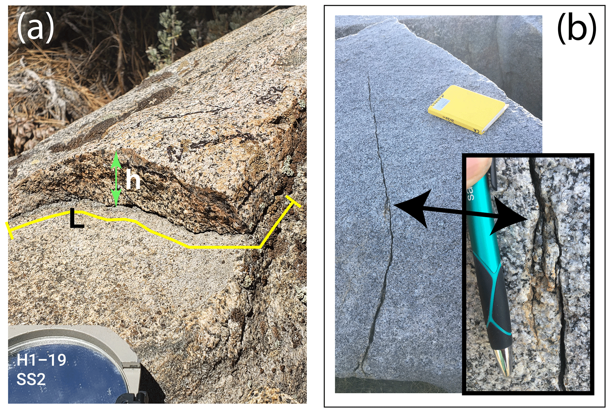
Figure 2(a) Example of the measurement of a surface exposure length (L; yellow line) of a fracture meeting the criteria in Table 1. The h refers to the location where sheet height would be measured for this surface-parallel fracture. (b) Example of fractures that may appear to be a single fracture (left) but upon close examination are in fact multiple fractures intersecting and/or separated by rock (right inset). Arrow points to the location of the inset image on the main image. Labeled compass in the foreground for scale and sample location information.
Last, and practically, the high abundance of fractures below this cutoff significantly increases the time required for fracture measurement. If these smaller fractures are of interest, they can be characterized with photographic analysis (not covered herein) or subjected to semi-quantification via an index (Sect. 5.2).
Importantly, in some applications, it may be appropriate that a larger minimum threshold in fracture length is chosen. However, in that case, fracture abundances in the rock will possibly dictate that significantly larger observation areas of the rock exposure need to be employed in order to obtain sufficient numbers of fractures to provide representative data (Sect. 4.2).
Regardless of the threshold length chosen for the study, two adjacent fractures separated by intact rock or bridges of cement are considered two fractures, even if at a distance they appear to be continuous (Fig. 2b). This practice results in repeatable measurement between multiple workers and provides the most accurate representation of past fracture growth and fracture connectivity in the rock body.
4.2 Determining how many fractures to measure
Most published fracture-focused studies provide no justification for the number of fractures they measure, begging the following question – is the dataset representative of the rock body? Studies of fracture statistics suggest a minimum of ∼200 fractures (Baecher, 1983) per site (as defined herein). For workers and situations that require more nuance or for which there is not ample rock surface to examine, we recommend an iterative approach. It is a long-recognized concept in fracture and rock mechanics that fracture size distributions are highly skewed and can be characterized by scale-independent power-law distributions (e.g., Davy et al., 2010; Hooker et al., 2014). Power-law distributions cross multiple orders of magnitude in frequency and scale, requiring up to an order of magnitude more observations to significantly define than the other more tightly defined distributions. Thus, the best practices to understand the commonly observed power-law distribution of fracture size can be leveraged in most cases to ensure that a representative fracture population has been measured in any given dataset (Ortega et al., 2006).
Here, it is recommended that to fully characterize the fractures for any site(s), outcrop(s), or feature(s) of interest, sufficient numbers of fractures should be measured such that if the fracture parameters are power-law-distributed, a statistically robust power-law distribution (p values <0.01) in fracture length or aperture can be estimated from the data. While other lognormal, exponential, and Weibull distributions have been proposed for various fracture datasets (e.g., Baecher, 1983), employing these distributions depends on pre-existing knowledge of the expected dataset, the very dataset in the process of being collected. Thus, unless there is prior documentation of fracture distributions at a particular site, the power-law distribution should suffice, and, in any case, power-law distributions require the most samples for significance compared to the other distributions.
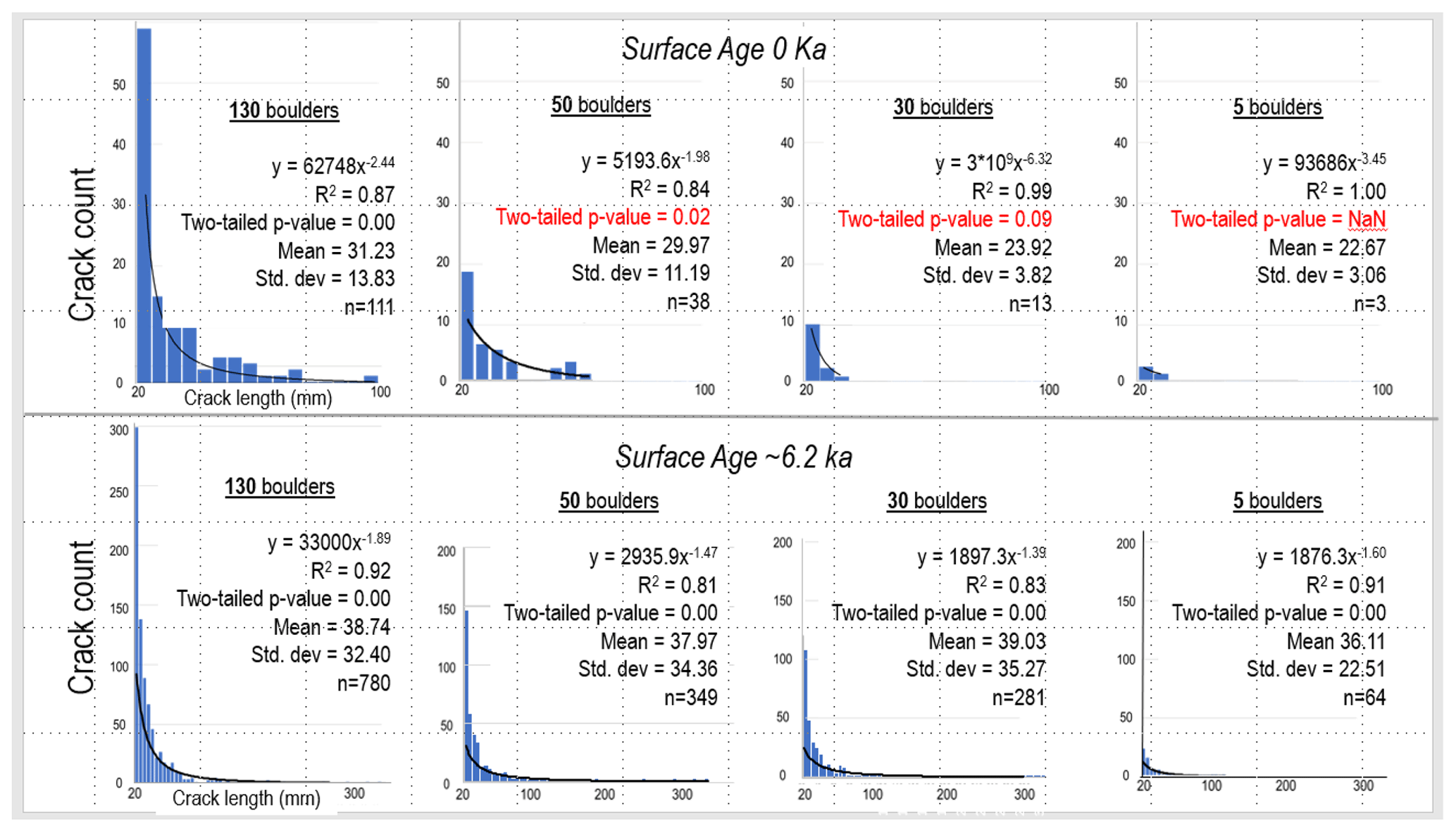
Figure 3Example histograms and statistics of fracture length data measured on the exposed surfaces of clasts 15–50 cm maximum diameter. The upper row shows data for clasts found on a modern ephemeral stream boulder bar. Clasts overall have a very low fracture number density. The lower row shows data for clasts on an ∼6 ka surface where the fracture number density is much higher. Note that it takes about 100 clasts to arrive at a statistically significant power-law distribution for the modern wash clasts but only five rocks for the rocks with higher fracture number densities. Producing histograms interactively as data are collected can help establish how many observation areas are necessary for a given site.
Thus, in practice, it will be an iterative process to determine the number of fractures required for any given dataset; but generally, on the order of 102 fractures are required (e.g., Zeeb et al., 2013) to reach a representative distribution (Fig. 3). When sufficient numbers of fractures have been measured to result in such a distribution, then it can be assumed that the population of measured fractures is representative of all fractures on the rock, outcrop, or group of rocks or outcrops with certain features. For example, if the goal of a study is to test the influence of rock type on fracture density, enough fractures must be measured to allow for a power-law distribution of fracture size for each of the rock types. That population of fractures can then be considered representative of the given rock type, and statistics on other fracture properties like width can also be reasonably interpreted as representative.
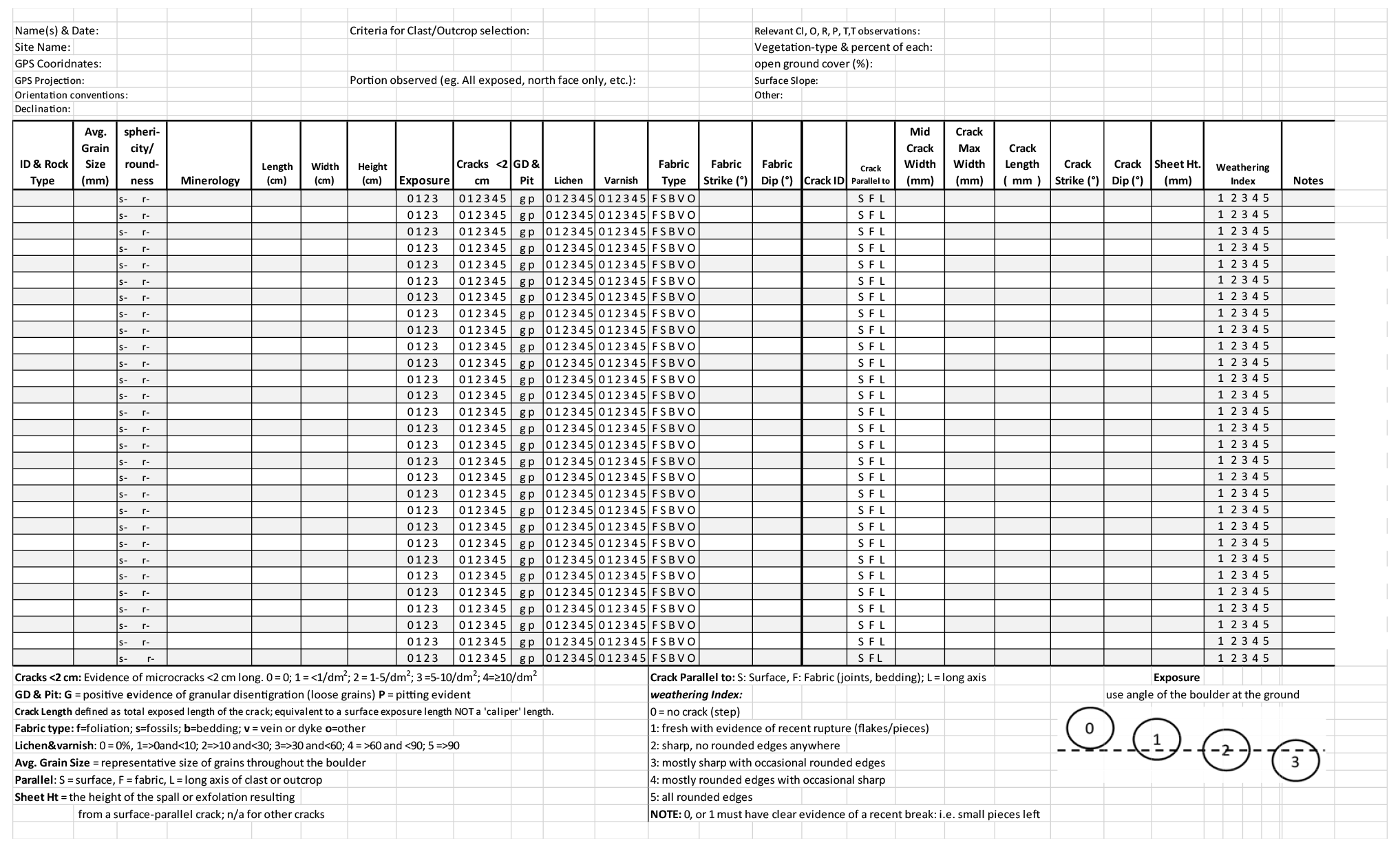
Figure 4Reduced size image of an 8.5” × 11” “fracture sheet” to be employed in the field to increase efficiency and to reduce “missing” data. Sheet templates for both clasts and outcrops that can be modified are provided in the Supplement as is a data-entry template.
If after ∼200 fractures are measured the power-law distribution is not met, then it is likely the dataset does not follow a power-law distribution and the number of measurements can be considered sufficient (Baecher, 1983). Some fracture arrays – particularly those formed at depth - have narrow (or “characteristic”) size distributions that are not well-approximated by power laws (e.g., Hooker et al., 2013). Another exception to the scale-independent power-law rule of thumb may be if there are abundant fracture terminations in infilling material. In this case, the size of the fracture (as defined by Table 1) is dictated by the spacing of the filled material bridges. Thus, fracture sets in rocks that contain abundant varnish or secondary precipitates like calcium carbonate may not follow the power-law rule, and a threshold number of ∼200 fractures per site should be employed.
An example of what the iterative process might look like is found in Fig. 3. In this example, all fractures were measured on the surface of 15–50 cm diameter granitic clasts selected along transects across both a modern wash bar (with few overall fractures per clast) and a ∼6 ka alluvial fan bar (with many fractures per clast). For the modern wash, after 5, 30, or 50 clasts, a statistically significant power-law distribution is not evident (Fig. 3). However, after 130 clasts, the fit of the power law falls below a p-value threshold of 0.01 with 111 fractures measured. Thus, measurements from around 130 clasts (∼100 fractures) were necessary to fully characterize fractures for that particular site. In contrast, the threshold p value is reached after only five clasts (64 fractures) for clasts with high fracture number density at the mid-Holocene age site; however, with more clasts examined, more variables per clast can be analyzed in the data. Thus, in order to evaluate different variables (like clast size or shape), the iterative process would repeat, but limiting the analysis to fractures found on clasts meeting the criteria of interest. In this example, a total of 130 clasts per surface were measured, enabling several subsets of data to be examined in order to test the influence of a range of clast properties on fracture characteristics. This iterative approach will give a reasonable indication of when enough samples have been collected, but determining the type of distribution and estimating the distribution parameters, i.e., the exponent of the power law, require more careful analysis that is covered below in Sect. 6.
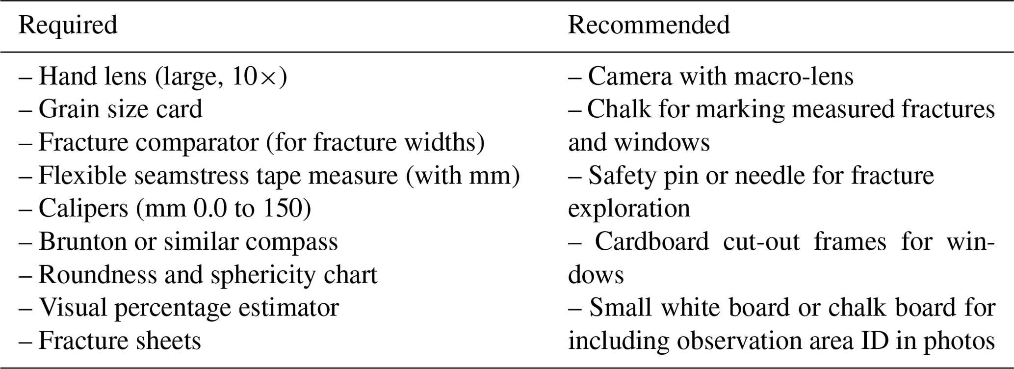
Here, a basic suite of field data (Table 2) is proposed for all observation areas and all fractures. Table 3 contains a list of recommended field equipment to make the measurements. The list of data in Table 2 was developed with the goal of allowing the worker to fully analyze their fracture data in the context of variables known from the literature to influence or reflect fracture in exposed rocks. Workers may choose to measure only some of these data if, for example, they have controlled for a particular metric through site or clast selection. As overall knowledge of fractures in surface environments grows, the suggested set of measured variables should also change, just as, for example, the components of the simple stream-power equation have evolved in fluvial geomorphology literature. The list of proposed fracture field methods is also focused on direct “observables” – without interpretation – that should universally apply across field areas. We readily acknowledge that additional items can and should be added to accommodate the needs of any specific study.
Table 2List of proposed data to collect for the rock observation area and for all fractures ≥2 cm in length.
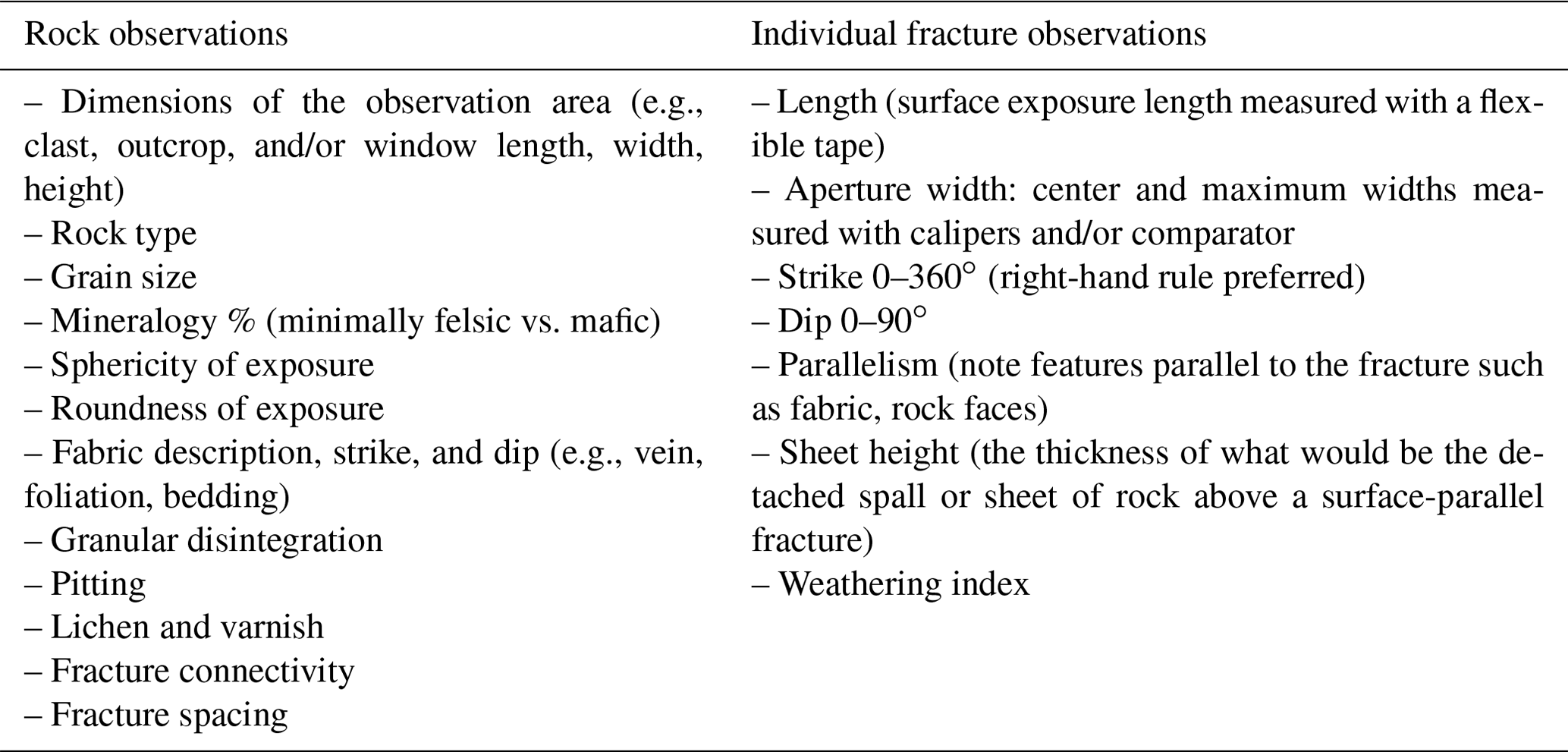
The metrics listed in Table 2 and the associated methods described below are designed to be applicable and translatable to both natural outcrops and individual clasts. While they may also be applicable to fractures found in quarries and road-cuts, such outcrops are prone to fracturing that has been anthropogenically induced by blasting, exhumation, and new environmental exposure (e.g., Ramulu et al., 2009; He et al., 2012).
5.1 The fracture sheet
A data collection template is provided that comprises all the proposed standard data, allowing efficient, complete, and detailed recording of all parameters while in the field (e.g., a “fracture sheet”; Fig. 4, with a digital version provided in the Supplement). The fracture sheet can and should be modified to include additional parameters relative to any study. The template provided here is structured based on our past experience so that each observation area's information (e.g., that of each clast, outcrop, or window) shares a row with the first fracture measured. Then, subsequent rows are employed for additional measured fractures on the same observation area. Each observation area and fracture is assigned unique identifiers to enable unambiguous reference in subsequent data analysis. Employing a window rather than an entire clast or outcrop as the observation area necessitates slightly different data collection, so two separate fracture sheets can be found in the Supplement.
The fracture sheet provides a header space for site metadata. Any observations that could elucidate the possible contributions of any state factor (cl, o, r, p, t, T) acting at the site should be recorded (e.g., the vegetation or topography of the site). This header area should also be employed to note any and all criteria or conventions used throughout the study. For example, the use of any convention, such as the right-hand rule for strike and dip measurements, should be noted in the header. The criteria employed to select clasts or outcrops (e.g., their size, composition) and the nature of the observation areas (e.g., only the north face of all clasts or entire exposed clast surface for all outcrops) should also be noted.
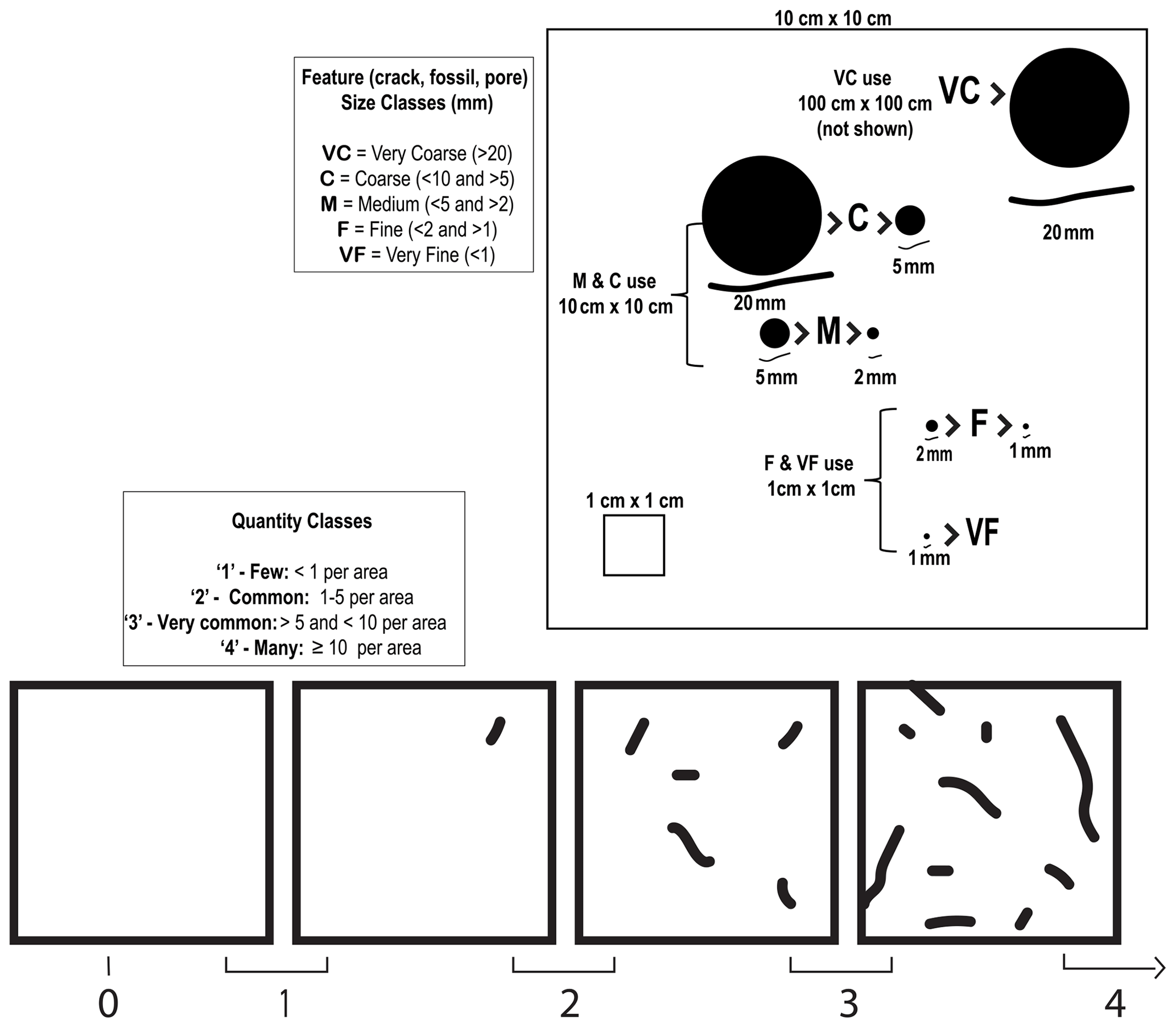
Figure 5Visual aid for estimating the abundance of “countable” rock features, including fractures. An index of 0–4 is assigned depending on the abundance of features within an average of any given observation area (ex: 10×10 cm) on the clast or window being examined. The area of observation is defined by the size of the features being measured. A 10 cm × 10 cm square is used for estimating the abundance of “fractures <2 cm” defined as fractures with lengths of >0.5 cm but <2 cm (see Sect. 5.2 for details of how to use the index). For features ≤0.5 cm, a 1 cm × 1 cm area would be employed, and for features ≥2 cm, a 1 × 1 m area. Ensure the image is printed to scale prior to use in the field (to scale figure available in the Supplement).
5.2 The use of semi-quantitative indices
It is recommended that indices be employed for many observations following similar existing semi-quantitative methods commonly employed in both soil sciences (e.g., Soil Survey Staff, 1999) and sedimentology (e.g., rounding and sorting). We have found in our experience that the use of indices, rather than precise measurements, is especially appropriate for fractures and fracture characteristics given the natural variation between different rocks. Also, high numbers of small or discontinuous features on rock surfaces frequently preclude their accurate counting within a reasonable amount of time: for example, counting all fractures <2 cm in length.
Two particularly useful generic “abundance” indices are defined here that are derived from those employed for quantifying the abundance of roots and pores in soils (Schoeneberger et al., 2012), whereby the quantity or coverage of specific elements or features is estimated within a specified area. For both, a “frame” is employed whose size is dependent on the size of the feature being observed (Fig. 5). Features that are ≤0.5 cm are observed in 1 cm2 frames, features >0.5 to <2 cm are observed in a 10 cm2 frame, and features ≥2 cm are observed in a 1 m2 frame. Cut-out stencils of these sizes may be constructed and employed. The observer imagines randomly placing the frame several times on any given portion of the observation area, noting the abundance of the feature of interest within the frame. The indices are based on the average value of abundance observed in any given such frame across the entire area of observation (e.g., the entire clast, the entire outcrop, or the outcrop window).
The first index scales from 0 to 4 and is applicable for “countable” features of interest in the research like small fractures, fossils, or large phenocrysts. The index is as follows: none – 0 (no visible features in any frame), few – 1 (<1 feature on average), common – 2 (≥1 and <5 features on average), very common – 3 (≥5 and <10 features on average), and many – 4 (≥10 features on average).
The second index scales from 0 to 5 and is employed for features that are not readily counted or consistent in size (like lichen, varnish, fine-grained mafic, or felsic minerals). In these cases, the index is based on the percentage of the rock surface covered by the feature: none – 0, very little – 1 (<10 %), little – 2 (≥10 % and <30 %), common – 3 (≥30 % and <60 %), very common – (≥60 % and <90 %), and dominant – 5 (≥90 %). A percentage estimator (Fig. 6) should always be employed to assign the index categories – even experienced field workers are subject to “quantity bias”.
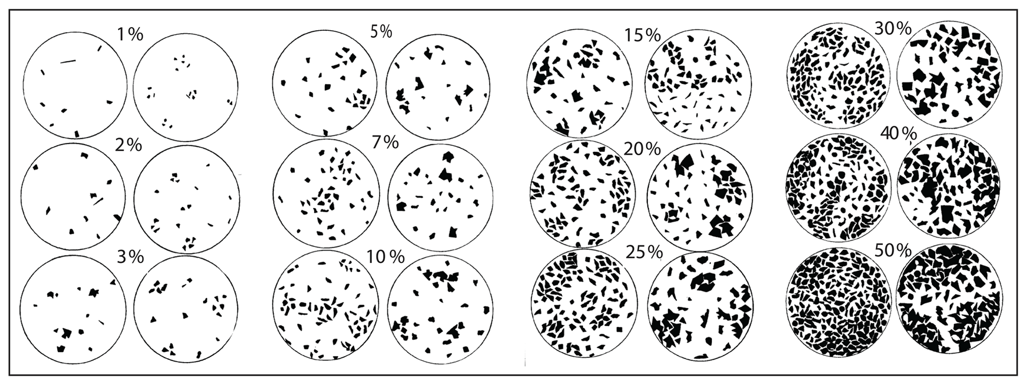
Figure 6A visual percent estimator (modified from Terry and Chilingar, 1955). An estimator should be employed in every estimate of percentages. See Sect. 5.2 for using the estimator to assign a percent coverage index to features that are not countable or vary in size (e.g., lichen coverage, fine mafic minerals).
5.3 Measuring rock characteristics
The following rock characteristics are measured for each observation area – each clast, outcrop, and/or window – that is employed in a study. Some fracture characteristics not captured in individual fracture measurements are also included. In particular, fracture connectivity and fracture spacing should be measured after all individual fractures within the observation area have been identified and measured.
5.3.1 Clast, outcrop, or window dimensions
Rock or outcrop size, aspect, and slope can impact stress loading through, for example, thermal stress distribution (e.g., Molaro et al., 2017). Or, for instance, natural outcrop height has been linked to its exposure age and/or erosion rates (e.g., Hancock and Kirwan, 2007; Anderson, 2002). The dimensions of the clast, outcrop, or window employed for fracture observations are also required for calculations of fracture number density and intensity (i.e., the number or length of fractures per unit area; see Sect. 6.1).
The length and width of planar windows are measured directly. If a window “bends” across multiple faces of the rock surface, then separate length and width measurements should be made for each face with a distinct aspect. These areas are then added together for fracture number density and intensity calculations.
The vast majority of rock clasts and outcrops found in nature have “cuboid” forms (Domokos et al., 2020). Thus, length, width, and height of individual clasts or outcrops may be reasonably employed to calculate the exposed surface area (see Sect. 6.1 for calculations). If clasts or outcrops are well-rounded, spherical or half-spherical surface areas can be employed, depending on burial.
For all dimension measurements regardless of rock shape, metrics are measured as point-to-point orthogonal measurements. By convention, length is measured parallel to the longest axis. Width is measured on the widest extent that is perpendicular to length, and height is measured vertically from the uppermost surface of the rock down to the ground surface. In past surface process work (e.g., Aldred et al., 2016; Eppes et al., 2010; McFadden et al., 2005), we have developed the rule of thumb that if a throughgoing fracture splits the rock into two pieces that remain in situ, it should still be considered one rock and measured accordingly. Such fractures formed in place and provide information about the fracturing history of the rock (e.g., D'arcy et al., 2014). If a clast or outcrop is spheroidal in shape, that should be noted for future surface area calculations.
For site preservation and to minimize geoheritage and environmental impacts, we believe that rocks should not be moved from their natural state; therefore, the height measurement of a highly embedded rock will only represent the height of the exposed rock surface above the ground. A metric derived to estimate the degree to which clasts are exposed versus embedded is provided in Sect. 5.3.8.
5.3.2 Sphericity and roundness
Sphericity and roundness from standard sedimentology practices (e.g., Krumbein and Sloss, 1951) provide metrics for rock shape. Shape can influence stress distribution in a mass and therefore a rock fracture. For example, generally, corners tend to concentrate stresses, and “corner fractures” are a recognized phenomenon in fracture mechanics (e.g., Kobayashi and Enetanya, 1976). Thus, this metric has been included as one to be measured for both outcrops and clasts.
Sphericity refers to the length by width ratio, or elongation, of the clast or outcrop, whereas roundness is a measure of angularity (Fig. 7). The roundness and sphericity designation for the square on the chart in Fig. 7 most closely matching the dominant shape of the entire clast or outcrop should be noted (ex. r-SR; s-SE). If a more precise rock shape analysis is needed, a modified Kirkbride device can be used to quantitatively measure rock roundness (see Cox et al., 2018, for device modifications and methodology).
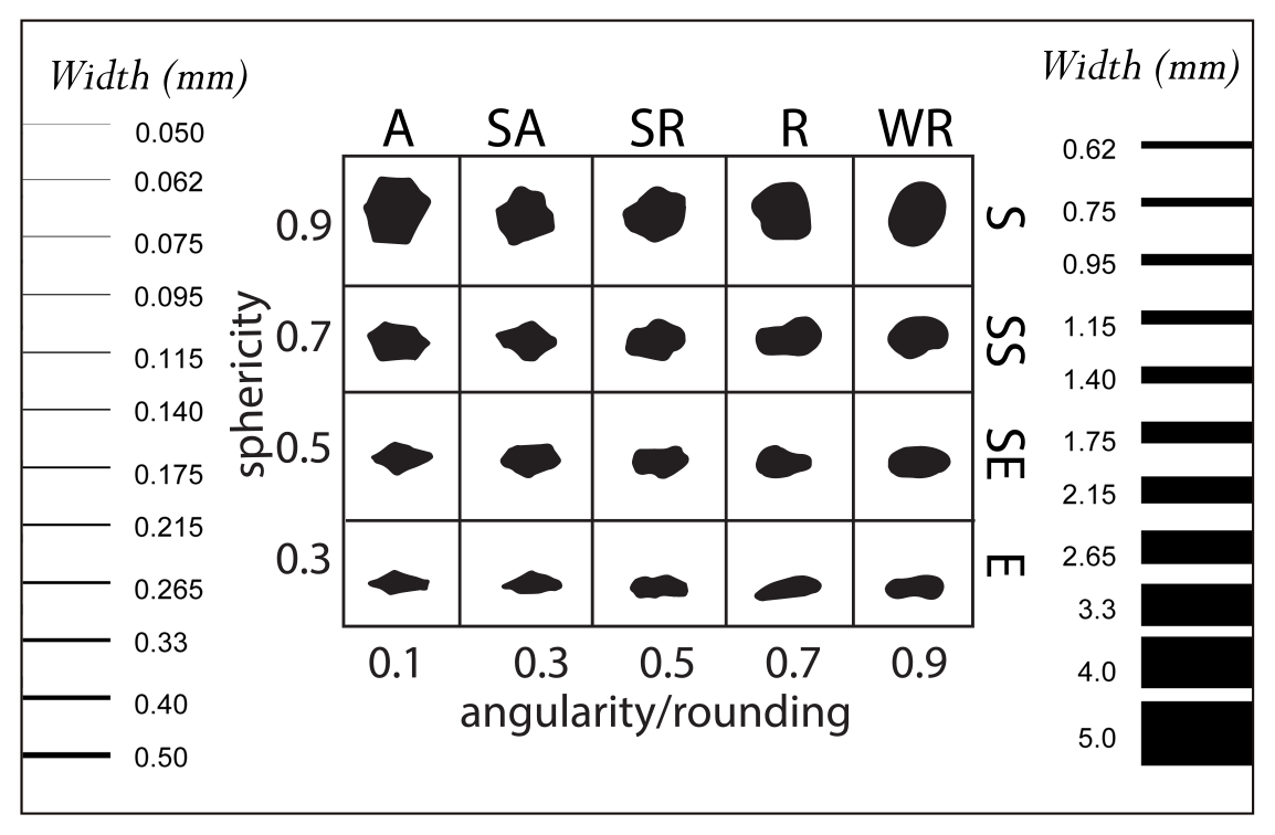
Figure 7Inset: roundness and sphericity chart – modified from Krumbein and Sloss (1951) to add the roundness and sphericity lettering. Roundness: A – angular; SA – subangular; SR – subrounded; R – rounded; WR – well-rounded. Sphericity: S – spherical; SS – subspherical; SE – sub-elongate; E – elongate. Edges: binned fracture width comparator after Ortega et al. (2006) whereby the width most closely matching the fracture aperture is noted. Note: a to-scale pdf is available in the Supplement; however, owing to printing and publication scaling, it is highly recommended to calibrate the comparator prior to using it in the field.
5.3.3 Grain size
Mean grain size can impact numerous fracture and stress characteristics including the proclivity for granular disintegration (Gomez-Heras et al., 2006), fracture toughness (Zhang et al., 2018), initial fracture length, thermal stress disequilibrium (Janio De Castro Lima and Paraguassú, 2004), and bulk elastic properties (Vazquez et al., 2015). The mean grain size is visually estimated by comparing the dominant size of individual grains or mineral crystals to a standard grain size card. This size can be reported as one average value for all minerals or different values for different suites of minerals (e.g., felsic vs. mafic), depending on the lithological assemblage(s) of the observation area(s) and the goals of the study.
5.3.4 Fabric and fracture filling
Here, the term “fabric” is employed to refer to any pre-existing (prior to weathering) primary or diagenetic planar, linear, or randomly oriented anisotropies within the rock comprising the outcrop or clast of interest. Fabric is most commonly observed as fossils or lithological bedding planes in sedimentary rocks and as crystal horizons or foliation structures in igneous or metamorphic rocks. Also, all rocks can have diagenetic mineral deposits within parts of otherwise open fractures or contain fully filled veins and dikes. Finding mineral deposits in open fractures points to a deeper origin. Rock fabric can impart anisotropy that influences rock strength, fluid flow, and fracture clustering, rates, and orientations (e.g., Nara and Kaneko, 2006; Zhou et al., 2022). Thus, any visible fabric type – as well as the strike(s) and dip(s) or trend(s) and plunge(s) – of each parallel or sub-parallel set is noted in the fracture sheet for each observation area. Through comparison of orientations, the extent to which fractures in the dataset are influenced by these fabrics can be determined.
5.3.5 Fractures <2 cm in length
Fractures <2 cm in length can comprise a significant portion of all fractures on a given rock exposure, particularly in coarse crystalline rock types (e.g., Alneasan and Behnia, 2021). Thus, it is recommended that an index is recorded (Sect. 5.2) using an observation frame that quantifies the abundance of fractures less than 2 cm in length (hereafter “small fractures”). In our experience, these data can help to explain, for example, fracture densities that are lower than expected when derived from the >2 cm fracture length dataset alone.
The approximate number of small fractures visible each time the frame is moved should be observed. A rough average of all theoretical frames should be taken, and the categories in Fig. 5 should be used to assign an abundance. For example, if there are generally either zero fractures or one small fracture in any given 10×10 cm frame, the abundance would be “1” – i.e., few, <1 per unit area.
5.3.6 Granular disintegration
Granular disintegration refers to evidence of active loss of individual crystals or grains due to fracturing along grain boundaries (i.e., sedimentary particles or igneous or metamorphic crystals). This feature is observed on the rock surface as individual grains or small clusters of grains of the rock that can be brushed away by hand. Granular disintegration is commonly observed in coarse igneous, metamorphic, and sedimentary rocks, and over the long term it leads to the accumulation of “grus” – sediment comprised of individual crystals or small clusters of a few crystals on the ground surface (Eppes and Griffing, 2010; Isherwood and Street, 1976; Gomez-Heras et al., 2006).
By necessity, this disintegration comprises the complete separation of intergranular fractures, and similar to fractures <2 cm, we have experienced that it can provide information about smaller-scale fracturing of the rock (e.g., Eppes et al., 2018). Because the fractures that comprise granular disintegration are typically too small to be readily measured in the field, its presence is assumed when loose grains are present on the rock surface. The worker marks affirmatively (circling the G on the fracture sheet) if there is evidence of granular disintegration on the rock surface of observation. If more detail is desired, an abundance index (e.g., Fig. 5) may be employed to quantify what percentage of the surface of observation contains loose grains.
5.3.7 Pitting
Pitting is the occurrence of small holes or fissures that form on the rock surface due to granular disintegration or to preferential chemical weathering of certain mineral types, typically feldspars and micas in silicate rocks. Pitting is distinct from granular disintegration as it is not necessarily “actively” occurring – i.e., pitting can exist without loose grains on the rock surface. It is included here as a rock property because of its possible linkage to intergranular fracturing. Furthermore, measuring the extent and depth of pitting due to chemical weathering has long been employed as a relative age dating tool in Quaternary geology applications (Burke and Birkeland, 1979).
Pitted surfaces form as individual grains become weathered and fall out or are dissolved or, for soluble rocks like carbonates, as entire rock regions are dissolved. Pitting is quantified either as present or absent (circling P on the fracture sheet) or as a quantity index (Figs. 4 and 5).
5.3.8 Clast exposure
This metric is used to record to what degree individual clasts appear to be exposed above the ground surface. Individual clasts are known to weather and erode from the upper rock surface down until they become “flat” rocks at the ground surface (e.g., Ollier, 1984), and the degree of embeddedness can impact preservation of fracture orientations (e.g., Aldred et al., 2015). We have found in our experience that surface exposure can be estimated as the amount and shape of a boulder's exposed surface that is currently not covered by loose sediment, vegetation, or other material, and it also relates to erosion rate in some settings. This exposure is grouped into four categories: 0 – the clast is sitting above the ground, and its sides curve downward toward the ground surface, almost meeting; 1 – the clast is partially covered, with sides curving downward toward the ground surface but not meeting; 2 – the clast is “half-covered”, with sides projecting roughly vertically into the ground surface; 3 – the clast has only one upward-facing side visible at the ground surface. In a field study, a correlation test on data from 300 boulders revealed a positive correlation of 0.66 between the indices and the fraction of boulder embeddedness (in vertical height) (Shaanan et al., 2023).
5.3.9 Lichen and varnish
Lichens and other plant life can act to push rocks apart during growth (Scarciglia et al., 2012) but have also been shown to strengthen rocks through infilling of voids or shielding from stress-inducing sunlight (Coombes et al., 2018). It is noted that lichens are living organisms that would be killed by removal. We have found that in order to determine if a lichen-coated lineation is in fact a measurable fracture (see Sect. 4.1), a large needle or straight pin may be employed to poke through the lichen into the possible void of the fracture.
Rock varnish (oxide staining that can appear as a dark gray–black or orange coating on rock and typically contains Fe or Mn oxides) is well-documented to evolve over time. The extent of varnish cover has frequently been employed as a relative age indicator, particularly in arid environments (e.g., McFadden and Hendricks, 1985; Macholdt et al., 2018). Thus, we infer that variations in varnish across the rock face can provide evidence of loss of surface material through in situ fracturing.
Lichen and varnish can come in many forms and be difficult to distinguish from each other and from primary rock minerals, hiding in fractures, in pitting holes, and atop mafic crystals. So, careful consideration of the types of lichen and varnish that may be found in field sites and close inspection with a hand lens is recommended. A fresher exposure of the rock surface can help in the identification of lichen and varnish relative to the natural rock composition and color. Due to the geodiversity impact, however, such exposures should not be made with force.
The quantities of lichen and varnish (secondary chemical precipitates deposited on the subaerial rock surface) visible on the rock observation surface are separately estimated using a visual percentage estimator (Fig. 6) and a quantity index is assigned (Fig. 5; Sect. 5.2).
5.3.10 Collecting samples for microfracture analyses
Rock microfractures (those not visible with hand lens in the field) play a central role in contributing to rock strength, anisotropy, and subsequent macrofracturing processes (Kranz, 1983; Anders et al., 2014). It is beyond the scope of the field-based methods presented herein to describe microfracture measurement and analysis, which continue to evolve (e.g., Griffiths et al., 2017; Healy et al., 2017). Instead, suggestions for rock sampling and placement of thin-section billets are provided.
Thin-section analysis of microfractures can be a time-consuming process, particularly when considering the per-capita rock volume examined. It is therefore extremely important to select rock or portions of rock that are precisely the rock type of interest and to carefully orient the sample. For loose clasts, an entire clast can be sampled and a thin-section billet processed in the lab. For larger clasts and bedrock, a smaller portion must be extracted. By sampling pieces that are already naturally detached or nearly detached, fracturing that arises due to chiseling or hammering is avoided. Epoxying samples prior to thin-section preparation helps preserve delicate features and avoids introducing artifacts. Extra-thick sections are recommended for microfracture work, since conventional sections are prone to developing fractures during grinding. For population sampling, continuous sections can be created of any length (Gomez and Laubach, 2006).
For both clasts and outcrops, the natural orientation of the sampled rock (its horizontal and azimuthal directions) is always marked on the specimen. The sample should be photographed prior to removing it from its location. It is essential to ensure that all permits are in place prior to sampling.
Similar to clast or outcrop selection, care must be taken when considering the location within the rock where the thin-section billet will be cut. Because microfracture strike and dip can be influenced by environmental, gravitational, and tectonic forces, both the depth and orientation of the billet should be noted and controlled for as appropriate for all samples compared within a single study.
5.3.11 Fracture connectivity
Fracture connectivity refers to the arrangement of fractures relative to each other. Connectivity has long been recognized as being key to rock strength and fluid flow (e.g., Rossen et al., 2000; Long and Witherspoon, 1985; Manzocchi, 2002; Viswanathan et al., 2022) and presumably contributes to rock erodibility, given that fractures must intersect for rock to erode. There is a large body of literature that addresses fracture connectivity and how to measure it (e.g., Berkowitz, 2002; Barton et al., 1993; Healy et al., 2017; Sanderson and Nixon, 2018), especially in the context of reservoirs and rock quality index studies. As yet, fracture connectivity has been less studied in the context of surface processes but likely holds high potential given its relationship to water access and erodibility. Here, the focus is on a simple rule-based observation of fracture intersection “nodes” (e.g., Barton and Hsieh, 1989; Manzocchi, 2002; Forstner and Laubach, 2022; Sanderson and Nixon, 2018) that comprise the basis for fracture network connectivity assessment (e.g., Andresen et al., 2013).
After all fractures within each observation area have been identified and measured (Sect. 5.4), all fracture links within the observation area should be counted and recorded by noting their relationship to other fractures (Fig. 8): dead end (I node), crossing (X node), and/or abutting without crossing (Y node). Numbers of nodes per area can then be used as a proxy for fracture connectivity. If fracture connectivity is of particular interest for the research, rule-based “contingent-mode” (C-node) intersections may also be added (Forstner and Laubach, 2022). An example of a C-node rule might be that if fractures >100 mm in length terminate within 10 mm of another fracture, its termination would be a C node. Another C-node definition could comprise intersection relations where visible connected traces are sealed with secondary minerals. These C nodes may be important when there are ambiguous at-depth relationships between fracture terminations (e.g., Fig. 2b).
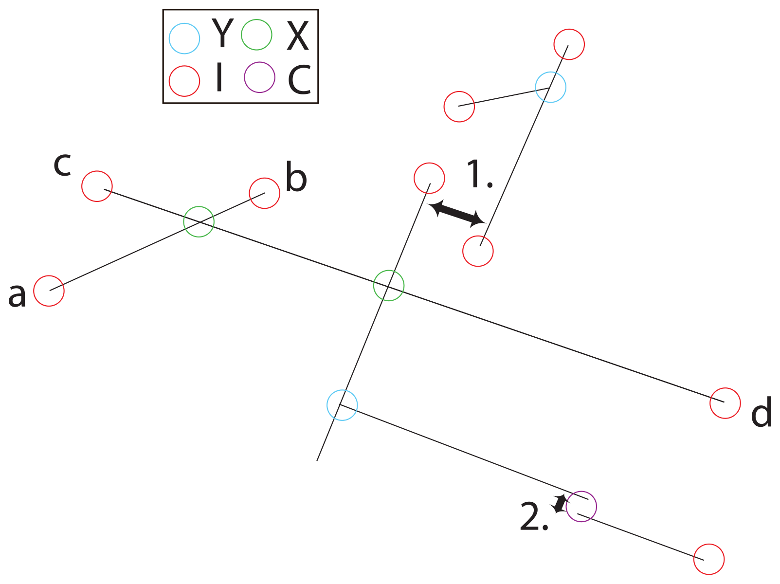
Figure 8Depiction of types of fracture intersection nodes. I nodes comprise fracture terminations with no connections. Y nodes are abutting fractures that do not cross. X nodes are fractures that cross. C nodes are “contingent nodes” defined by the user. In this example the rule is related to the distance between I nodes. For no. 1, the distance is wider than the criteria, so the terminations are designated as I nodes. For no. 2, the distance is within the limits, and the “connection” is designated as a C node.
5.3.12 Fracture spatial arrangement
In addition to overall fracture density, intensity, and connectivity, the arrangement of fractures in space (e.g., evenly spaced, random, clustered in space) can impact loci of rock mass weakness, fluid flow, and landscape morphology. The study by Laubach et al. (2018) comprises a special issue of the Journal of Structural Geology devoted to spatial arrangement of fractures, and much work has been published since. The mathematical analysis of spatial arrangement and rigorous identification of clustering are beyond the scope of this field guide. Software is freely available for analyzing one-dimensional fracture arrangement along scanlines (Marrett et al., 2018) and for analysis of trace patterns in two dimensions (Corrêa et al., 2022; Shakiba et al., 2023).
For scanline-based methods, following similar methods as those used for locating windows (Sect. 3.4), lines should be established across representative parts, or the center, of each observation area. For 1D analysis, good practice is to establish at least two perpendicular lines to capture different orientations of fractures, but the optimal number and configuration depend on the pattern under investigation. A tape or other linear measuring tool is then arranged along the lines, and, beginning with the edge of the observation area as distance 0, the distance along the tape of each fracture is noted (in other words, the sequence of spacing between fractures is recorded), with each measurement linked to the fracture ID already established for that fracture on the fracture sheet. If fractures are already marked with chalk, we find that this is an easy process. In that way, the size of each fracture and its adjacent distances are noted (analysis procedures allow weighting by fracture height, length, or aperture). As with any measure of fracture aggregate properties such as intensity or connectivity, for fractures having a wide range of sizes, arrangement results depend on the size range of fractures included in the analysis (scale-dependent) (e.g., Ortega et al., 2006). These spatial arrangement data can go on the back of the fracture sheet.
5.4 Individual fracture characteristics
The following properties are measured for each fracture found within the observation area that meets all the fracture selection criteria listed in Table 1. In order to keep track, we have found from experience that it is useful to mark fractures with chalk within the observation area after you have made their appropriate measurements.
5.4.1 Length
Fracture length is measured for the entire surface exposure length of the fracture, i.e., around corners and up and down rock topography (Fig. 2a). We have found these surface exposure distances to be the most repeatable and representative for the amount of fracture exposed on the rock surface (Aldred et al., 2016). Measurements can be made with flexible seamstress tape to follow the curve of a fracture's exposure on the rock surface. Length is only measured where there is an open void (Fig. 2b; Sect. 4.1) because to measure across bridges of secondary cemented material or rock would be to infer future fracture propagation that has not yet occurred. By only measuring the open portion of voids, the user avoids arbitrary interpretation of possible behavior. Thus, if a seemingly continuous fracture (Fig. 2b, left inset) is in fact separated by bridges of solid rock (Fig. 2b, right inset), then these should be measured as two different fractures and their lengths should terminate at the rock bridges (Sect. 4.1). The inset in Fig. 2b reveals four fractures possibly meeting all Table 1 criteria. If two fractures intersect in X or Y nodes (Fig. 8), each fracture is defined by its own distinct strike, and the full length of the full open fracture with that strike is measured (e.g., the length of segments a–b and c–d in Fig. 8).
Importantly, when using a window approach to rock observation area, both the total length of the fracture extending beyond the window and the total length within the window should be recorded. The latter is employed in fracture intensity calculations (Sect. 6.1); the former provides representative information about all fracture lengths on the rock being measured.
5.4.2 Width
Fracture aperture widths (hereafter, “widths”) can impact both the strength and permeability of rock. Generally, they scale with fracture length and, thus, can possibly reflect the innate subcritical cracking parameters of the rock (Olson, 2004). Fracture widths typically vary along their exposure and pinch out at fracture tips. Determining an average or representative width within a single fracture can thus be somewhat arbitrary and subject to bias. Locating the widest aperture is less subject to bias and can also provide information about fracturing processes (for example, the widest aperture in a series of mechanically interacting en echelon fractures should be in the center fracture; Anderson, 2005). Also, we find that the center of the open fracture is an objectively repeatable location and also where the fracture might be expected mechanistically to be the widest. However, given that this relationship can become complicated as fractures fill or branch, unless there is reason to do otherwise, we recommend the rule of thumb to record fracture width at both the midpoint of the measured length of the exposed fracture and its maximum width along its exposure.
We assert that in order to delineate the fracture – as opposed to measuring subsequent weathering or erosion – width measurements should only be made in regions of the fracture where fracture walls are parallel or sub-parallel (e.g., green arrows in Fig. 9), avoiding locations where fracture edges have been obviously rounded by erosion or chemical weathering or where large pieces have been chipped off or are missing (e.g., red arrows in Fig. 9). If it is unclear if a portion of the fracture has chipped off (e.g., orange arrow in Fig. 9), a notation can be made and employed later to eliminate potential outliers in the dataset. Fractures greater than about 3 mm in width can be easily measured by inserting the back-blades of digital calipers into the widest opening of the fracture. For narrower fractures, a logarithmically binned “crack comparator” (Fig. 7) is recommended (Ortega et al., 2006), whereby the line on the comparator most closely matching the fracture aperture is chosen.
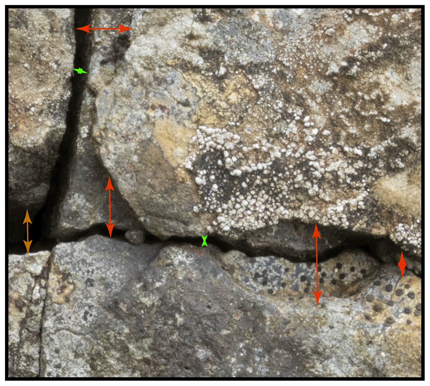
Figure 9Examples of aperture transects that are appropriate for measurement of fracture aperture widths (green) and transects where there is evidence that the fracture walls have been eroded or chipped and therefore should not be employed for a width measurement (red). In cases where it is not clear if erosion or chipping has occurred (orange), a note can be made for the fracture width to possibly eliminate outliers during data analysis.
5.4.3 Strike and dip
Fracture orientation (i.e., strike and dip) is a function of the orientation of existing anisotropy within the rock and the orientation of the principal stresses that drove its propagation (e.g., Anderson, 2005). Fracture orientations are commonly related to tectonic forces; however, both gravitational and environmental stresses can also be directional (e.g., St. Clair et al., 2015; McFadden et al., 2005). When fractures are growing at subcritical rates, they can lengthen through a series of “jumps” that link parallel or sub-parallel smaller fractures (e.g., Ma et al., 2023). The following suggestions are for research aimed not at characterizing these small millimeter- to centimeter-scale heterogeneities but rather identifying major stresses and heterogeneity in the entire rock body.
Fracture orientation is measured with a geological compass or similar tool that has both azimuthal direction and inclinometer functionality. When measuring strike and dip of fractures, we find it is helpful to visualize how the fracture plane intersects the rock surface, as if slipping a sheet of paper into the “file folder” of the fracture. For larger fractures, weathering and erosion may have resulted in loss of rock along the upper edge of the fracture, so it is imperative to measure the angle at the interior of the fracture where its walls are parallel (Fig. 9) to avoid measuring the angle of the eroded face instead.
Fractures grow until they intersect other fractures and/or branch, segment, and link. If fractures appear to intersect, branch, or link (i.e., two connected planar voids with noticeably different orientations joined by a sharp angle), their lengths should be measured separately as should their orientations (e.g., two strikes and dips) as previously mentioned. This phenomenon is in some cases evident in 2D spatial analysis that takes length scales into account (e.g., Corrêa et al., 2022). For fractures that meander around millimeter- to centimeter-scale heterogeneities like phenocrysts or fossils, the overall trend is measured. A 1 to 10 rule of thumb (Sect. 4.1) can be used, whereby, as long as the “jog” in the fracture orientation is of the fracture length, it is not measured.
Fracture-tip propagation direction may also slowly change as the orientation of external stresses or internal stress concentrations change within the rock mass. For curvilinear fractures, the average orientation can be measured as the orientation of the non-curved plane whose ends are defined by the ends of the fracture. Alternatively, the fracture curvilinear plane may be subdivided into roughly linear planes and each orientation measured. If this latter approach is taken, the intersection should be marked as a node and two lengths recorded. It is important to note which method was employed and to remain consistent for all measurements, as no widely acknowledged rule of thumb exists to our knowledge for this measurement.
There are numerous commonly employed conventions for measurements of strike and dip. If the worker is consistent and clear in the use of their preferred convention and in the presentation of their data, any are acceptable. If the worker has no such prior habits, we recommend, from our experience, that recording strikes as an azimuthal orientation from 0–359∘ and dip angle as an angle deviation from horizontal of 0–90∘ makes data analysis easier than recording, for example, direction by quadrant. For dip direction, we recommend that a convention such as the “right-hand rule” be employed whereby the dip direction is always known from the orientation of the strike alone. For example, the right-hand rule states that the down-dip direction is always to the right of the measured and recorded strike when the observer is facing the same direction of the strike. Therefore, the strike that is recorded is the one whereby the dip direction is always +90∘ clockwise (to the right) from the strike direction.
5.4.4 Fracture parallelism
Noting the parallelism of the fractures can help to better understand the origins of the population of fractures at a site. Parallelism is common because fractures often follow rock heterogeneities or anisotropies such as bedding, foliation, veins, or even the rock surface (e.g., McFadden et al., 2005). Fractures in a single bedrock outcrop or clast are also commonly parallel because they have formed due to external stress loading with a consistent orientation (e.g., those influenced by regional tectonics or directional insolation). Thus, noting parallelism may help to distinguish the origins of fractures, though not always. For example, “surface-parallel fractures” (e.g., Fig. 2a) – commonly referred to as exfoliation, sheeting joints (e.g., Martel, 2017), or spalling – vary dramatically in scale and can have origins related to several different factors including tectonic–topographic interactions (Martel, 2006), chemical weathering and volumetric expansion (Røyne et al., 2008), and thermal stresses related to insolation (e.g., Lamp et al., 2017; Collins and Stock, 2016) and fire (e.g., Buckman et al., 2021). Likewise, fractures having a strong preferred orientation parallel to topographic features like escarpments or stream channels may predate the topography and have localized the geomorphic feature, or they may postdate the feature and themselves be a response to topographic loads (e.g., Molnar, 2004). For this reason, fracture pattern sampling that seeks to avoid or characterize these effects should include exposures distant from such ambiguous situations (i.e., close to and distant from topographic features).
In the fracture sheet, features to which the fracture is parallel should be documented. We find that a visual inspection will suffice for most applications, but for applications where more precision is needed, the fracture may be considered parallel if the strike and dip of a fracture are within ± 10∘ of the orientation of the feature (the rock's long axis, its fabric, or its outer surface). We base this cutoff on the ± 4–7∘ strike and dip orientation precision of a typical Brunton compass under ideal measuring conditions (e.g., Whitmeyer et al., 2019). A fracture may be parallel to more than one feature in the rock. Categories may be added as necessary for rocks with other repeating features unique to the field site (fossils, veins, etc.). Assertions of parallelism (or similar) are a potential source of ambiguity, so careful consistency in the quantification of the basis of the claim is needed.
5.4.5 Sheet height
Surface-parallel fractures naturally detach “sheets” of rock between the fracture and the rock surface (h in Fig. 2a). Sheet height is thus only measured for surface-parallel fractures. We infer that the thickness of these sheets may be of interest for understanding the size of sediment produced from the fracture or for understanding the stresses that produced the fracture. We provide the rule of thumb that sheet height is measured using calipers at the location of the maximum height of the sheet because thin edges often break off and vary. To limit these measurements to those that have likely formed in situ as related to the current morphology of the rock, another rule of thumb we have employed is to only measure sheets that would result in removal of <10 % from the outer surface of the rock downward into the dimension(s) of the rock face(s) to which they are perpendicular.
5.4.6 Weathering index
Rock fracture is ultimately a molecular-scale bond-breaking process; so, when fractures propagate, they initially form a razor-sharp lip or edge where their two planes intersect the rock surface. Over time, these edges naturally round through subsequent chemical and physical weathering, erosion, and abrasion (e.g., regions of the red arrows in Fig. 9). Fracture tips may also blunt through time, but that observation may be complicated by the presence of mineral deposits. Following similar research that has demonstrated time-dependent changes in rock surface morphology due to such weathering processes (e.g., Shobe et al., 2017; Gómez-Pujol et al., 2006; McCarroll, 1991), we established an index of the relative degree of such rounding along a fracture edge (rather than fracture tip) to be noted in the fracture sheet:
-
fresh with evidence of recent rupture (flakes and/or pieces still present, but not attached);
-
sharp, no rounded edges anywhere;
-
mostly sharp with occasional rounded edges;
-
mostly rounded edges with occasional sharp edges;
-
all rounded edges.
When the data collection has been completed, it is necessary to provide statistics. For initial data exploration, general properties may be calculated for rock and fracture data like the mean, median, variance, skewness, kurtosis, and overall “appearance” of distributions. Data can be compared using normal cross-plots, or quantile–quantile plots, as well as standard correlation analysis. For categorical data, normal analytical techniques (histograms, discrete correlation analysis, etc.) can be applied. As with all heavy-tailed data, the median is preferred over the mean value to understand a characteristic value – though power-law-distributed data generally do not have a characteristic dimension. Distribution characterization is discussed in Sect. 1.3. 2D spatial analysis methods can also be applied to entire outcrops or clasts or to subdivisions of these features (Corrêa, et al., 2022; Shakiba et al., 2023). These methods are well-suited to large outcrops and well-exposed fracture arrays.
6.1 Fracture number density and fracture intensity
Here, following a large portion of fracture mechanics literature and for clarity, the term “fracture number density” is employed to refer to the number of fractures per unit area (e.g., no. fractures m−2) and the term “fracture intensity” to the sum length of all fractures per unit area (e.g., cm m−2). However, it is crucial to note that these terms are frequently defined differently and in inconsistent ways across disciplines and even within disciplines (e.g., Barthélémy et al., 2009; Narr and Lerche, 1984; Ortega et al., 2006; Dershowitz and Herda, 1992). To avoid confusion, it is imperative that workers clearly define their usage in each work. In particular, fracture intensity is scale-dependent. If the outcrops or clasts on which fractures are measured vary greatly in size, intensity calculations that account for the fracture distribution may be appropriate (e.g., Ortega et al., 2006).
In the suggested simple use herein, the area refers to the surface area of an observation area. For fractures measured in windows (Sect. 3.4), the length of fractures only within the window is used, and the area of the window (e.g., 10 cm × 10 cm) is used for the calculations. For loose clasts and outcrops, the appropriate calculation of surface area will depend on the shape and angularity of the rock. For most rocks, calculations for the surface area of the exposed sides of a rectangular cuboid () are appropriate.
6.2 Circular data
Standard “linear” statistics cannot be employed for circular data. Instead, circular statistical and plotting software is used for the visualization and analysis of strike and dip data. The statistics employed by such software are typically based on established circular statistical research methods (e.g., Mardia and Jupp, 1972; Fisher, 1993). The following statistics are from that work and are useful in reporting strike and dip data.
The mean resultant direction (also called the vector mean or mean vector) is analogous to the slope in a linear regression. Circular variance can be quantified using either a Rayleigh uniformity test (for single-mode datasets) or a Rao spacing test (for datasets with multiple modes), whereby p values <0.05 indicate non-random orientations. If p values for these tests are below a threshold (e.g., <0.05), then data are considered non-uniform or non-random.
The Rayleigh statistic is based on a von Mises distribution (i.e., a normal distribution for circular data) of data about a single mean (i.e., unimodal data). Therefore, for multi-modal data, the variance might be high, but nevertheless, the data might be non-uniform. The Rayleigh uniformity test calculates the probability of the null hypothesis that the data are distributed in a uniform manner. Again, this test is based on statistical parameters that assume that the data are clustered about a single mean.
Rao's spacing test is also a test for the null hypothesis that the data are uniformly distributed; however, the Rao statistic examines the spacing between adjacent points to see if they are roughly equal (random with a spacing of ) around the circle. Thus, Rao's spacing test is appropriate for multi-modal data and may find statistical significance where other tests do not.
Here we present a simple, brief example of how the presented methods promote consistency of results across users in fracture measurements; providing a full case study is beyond the scope of this paper. We provided minimal training (one demonstration with some minor oversight of initial work) to four groups of two students each. The fifth pair of workers included a scientist who had logged over 500+ hours of experience using the standardized methods. Each of the five groups followed the methods to measure the length and abundance of fractures on boulders (15–50 cm in length) on the same geomorphic surface (a 6000-year-old alluvial fan in Owens Valley California, primarily comprised of granitic rock types). Each group followed the methods described herein for rock and fracture selection and measurements. As such, the results from each group could be compared not only for fracture selection and measurements, but also for observation area selection – a key component of collecting data that are representative of a particular site.
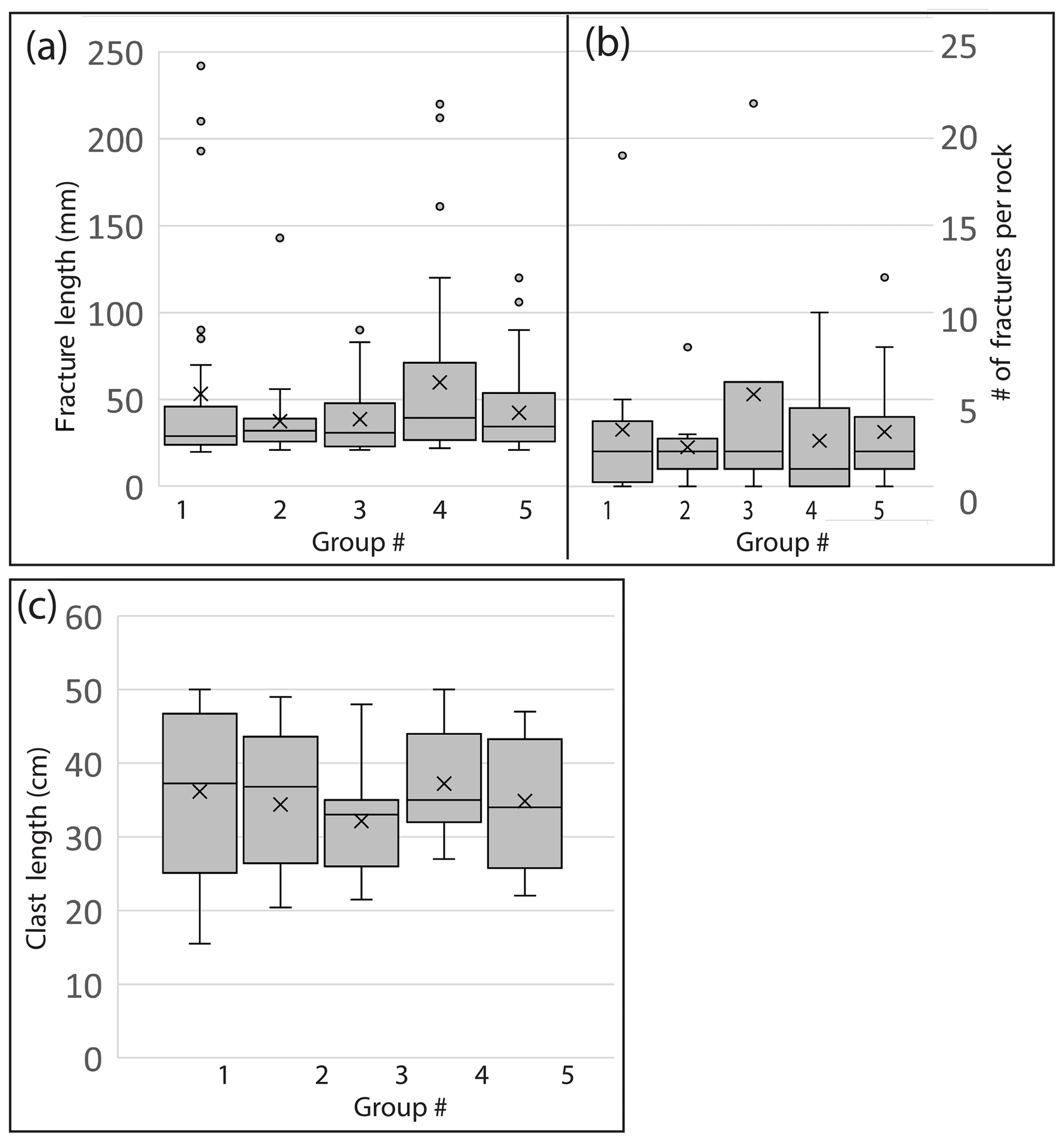
Figure 10Box-and-whisker plots of case example data collected by five different pairs of workers on the same geomorphic surface. X symbols mark the means. Groups 1–4 were novice workers. Group 5 comprised one experienced worker. (a) Fracture lengths. (b) Fractures per rock. (c) Clast length.
We find that the data collected by each of the groups for fracture length, number of fractures per rock, and rock size are statistically indistinguishable by a Student's t test (all pairs of p values >0.1; Fig. 10). Also, there is no consistent difference between measurements made by the novice groups and those of the trained group. The mean fracture lengths from the four novice groups (37±23 to 59±51 mm) span across the mean collected by the well-trained group (42±22 mm; Supplement), as does the number of fractures per rock (2±2 to 6±8 for novice groups compared to 3±3 for the trained group). With only one exception (fracture length for Group 1), variance between groups does not range by more than a factor of 3 in any of the data – a common rule of thumb for the threshold of “similar” variance between small datasets. Overall, especially given the relatively small size of the datasets (∼ 10–20 rocks and ∼ 40–60 fractures each), this comparison suggests that the results using the standardized methods are reproducible, even with novice workers with minimal training. A full case study and analysis would be required to fully and quantitatively evaluate all of the procedures presented herein.
The methods proposed herein comprise a “first stab” at standardization of field data collected in rock fracture research surrounding surface processes and weathering-based geologic problems. The outlined methods comprise best practices derived in large part from existing work in the context of structural geology and geotechnical engineering. They also comprise general guidance and nuances developed from experiences (and mistakes) over the last 2 decades of fracture-focused field research applied to geomorphology and soil science. We readily acknowledge that additional, fewer, or altered methods may be appropriate for some applications. Nevertheless, it is our hope that providing these rule-based, detailed, accessible, standardized procedures for gathering and reporting field-based fracture data will open the door to rapidly building a rigorous galaxy of new datasets as these guidelines and methods become more widely adopted. In turn, they may enable future workers to better compare and merge fracture data across a wide range of studies. Doing so will permit future refinements not only of the methods themselves, but also and most importantly of our understanding of rock fracture. Compiling such a standardized global dataset is the best hope for fully characterizing the role and nature of fractures in Earth surface systems and processes.
All data presented in the paper are available in the Supplement.
The supplement related to this article is available online at: https://doi.org/10.5194/esurf-12-35-2024-supplement.
MCE spearheaded the evolution of the development of the guiding principles and methods described herein as well as writing of the paper. AR and SEL significantly contributed to the editing of the paper content and expanding the breadth and depth of its applicability and approaches. JA, SB, MPD, SGE, FM, SP, MR, and US all extensively participated in field campaigns during which the methods were developed and refined, and they contributed to editing the paper and editing and development of figures. MM, AR, and RK contributed to the development of theoretical statistical analysis practices that are outlined in the document and the editing of the paper.
The contact author has declared that none of the authors has any competing interests.
Publisher's note: Copernicus Publications remains neutral with regard to jurisdictional claims made in the text, published maps, institutional affiliations, or any other geographical representation in this paper. While Copernicus Publications makes every effort to include appropriate place names, the final responsibility lies with the authors.
The body of knowledge presented herein was derived in large part over the course of research funded by the National Science Foundation and NASA. Several photographs in figures were cropped and employed with permission from Marek Ranis, artist-in-residence for the NSF (no. 1744864). We thank Claire Bossennec and Colin Stark for their constructive reviews. In addition, the authors wish to acknowledge the contributions from countless undergraduate and graduate students who contributed to the application and development of these methods in classes taught by MCE at the University of North Carolina at Charlotte.
This research has been supported by the National Science Foundation under grant nos. EAR 0844335 (with supplement nos. 844401, 0705277), 1744864, and NSF-BSF 1839148, as well as the NASA ROSES Mars Data Analysis Program under award no. NNX09AI43G.
This paper was edited by Richard Gloaguen and reviewed by Claire Bossennec, Adedibu Sunny Akingboye, C. P. Stark, and one anonymous referee.
Aich, S. and Gross, M. R.: Geospatial analysis of the association between bedrock fractures and vegetation in an arid environment, Int. J. Remote Sens., 29, 6937–6955, https://doi.org/10.1080/01431160802220185, 2008.
Al-Fahmi, M. M., Hooker, J. N., Al-Mojel, A. S., and Cartwright, J. A.: New scaling of fractures in a giant carbonate platform from outcrops and subsurface, J. Struct. Geol., 140, 104142, https://doi.org/10.1016/j.jsg.2020.104142, 2020.
Aldred, J., Eppes, M. C., Aquino, K., Deal, R., Garbini, J., Swami, S., Tuttle, A., and Xanthos, G.: The influence of solar-induced thermal stresses on the mechanical weathering of rocks in humid mid-latitudes, Earth Surf. Proc. Land., 41, 603–614, 2015.
Alneasan, M. and Behnia, M.: An experimental investigation on tensile fracturing of brittle rocks by considering the effect of grain size and mineralogical composition, Int. J. Rock Mech. Min., 137, 104570, https://doi.org/10.1016/j.ijrmms.2020.104570, 2021.
Anders, M. H., Laubach, S. E., and Scholz, C. H.: Microfractures: a review, J. Struct. Geol., 69, 377–394, https://doi.org/10.1016/j.jsg.2014.05.011, 2014.
Anderson, R. S.: Modeling the tor-dotted crests, bedrock edges, and parabolic profiles of high alpine surfaces of the Wind River Range, Wyoming, Geomorphology, 46, 35–58, 2002.
Anderson, T. L.: Fracture Mechanics: Fundamentals and Applications, third edn., Taylor & Francis Group, Boca Raton, FL, ISBN10 9781498728133, 2005.
Andresen, C. A., Hansen, A., Le Goc, R., Davy, P., and Hope, S. M.: Topology of fracture networks, AIP Conf. Proc., 1, 7, https://doi.org/10.3389/fphy.2013.00007, 2013.
Andrews, B. J., Roberts, J. J., Shipton, Z. K., Bigi, S., Tartarello, M. C., and Johnson, G.: How do we see fractures? Quantifying subjective bias in fracture data collection, Solid Earth, 10, 487–516, https://doi.org/10.5194/se-10-487-2019, 2019.
Andričević, P., Sellwood, E. L., Freiesleben, T., Hidy, A. J., Kook, M., Eppes, M. C., and Jain, M.: Dating fractures using luminescence, Earth Planet. Sc. Lett., 624, 118461, https://doi.org/10.1016/j.epsl.2023.118461, 2023.
ASTM: D7012-14: Standard Test Methods for Compressive Strength and Elastic Moduli of Intact Rock Core Specimens Under Varying States of Stress and Temperatures, ASTM D7012-14e1, 2017.
Atkinson, B. K.: Fracture Mechanics of Rock, Academic Press Geology Series, Academic Press Inc., Orlando, Florida, https://doi.org/10.1016/C2009-0-21691-6, 1987.
Ayatollahi, M. R. and Akbardoost, J.: Size and geometry effects on rock fracture toughness: Mode I fracture, Rock Mech. Rock Eng., 47, 677–687, https://doi.org/10.1007/s00603-013-0430-7, 2014.
Aydin, A. and Basu, A.: The Schmidt hammer in rock material characterization, Eng. Geol., 81, 1–14, https://doi.org/10.1016/j.enggeo.2005.06.006, 2005.
Baecher, G. B.: Statistical analysis of rock mass fracturing, J. Int. Ass. Math. Geol., 15, 329–348, https://doi.org/10.1007/BF01036074, 1983.
Balco, G.: Technical note: A prototype transparent-middle-layer data management and analysis infrastructure for cosmogenic-nuclide exposure dating, Geochronology, 2, 169–175, https://doi.org/10.5194/gchron-2-169-2020, 2020.
Barthélémy, J.-F., Guiton, M. L. E., and Daniel, J.-M.: Estimates of fracture density and uncertainties from well data, Int. J. Rock Mech. Min., 46, 590–603, https://doi.org/10.1016/j.ijrmms.2008.08.003, 2009.
Barton, C. C. and Hsieh, P. A.: Physical and Hydrologic-Flow Properties of Fractures: Las Vegas, Nevada – Zion Canyon, Utah – Grand Canyon, Arizona – Yucca Mountain, Nevada, 20–24 July 1989 (Field Trip Guidebook T385), American Geophysical Union, Washington, D. C., ISBN 9780875906508, 1989.
Barton, C. C., Larsen, E., Page, W. R., and Howard, T. M.: Characterizing fractured rock for fluid-flow, geomechanical, and paleostress modeling: Methods and preliminary results from Yucca Mountain, Nevada, United States, 74 pp., US Geological Survey, Denver, CO (United States), https://doi.org/10.2172/145208, 1993.
Bell, F. G.: Engineering Geology, 2nd edition, Butterworth-Heinemann Press, Burlington, MA, USA, 581 pp., ISBN 978-0-7506-8077-6, 2007.
Berberich, S.: A chronosequence of cracking in Mill Creek, California, Geography and Earth Sciences, The University of North Carolina Charlotte, ProQuest, 2478766717, 2020.
Berkowitz, B.: Characterizing flow and transport in fractured geological media: A review, Adv. Water Resour., 25, 861–884, https://doi.org/10.1016/S0309-1708(02)00042-8, 2002.
Betlem, P., Birchall, T., Lord, G., Oldfield, S., Nakken, L., Ogata, K., and Senger, K.: High resolution digital outcrop model of faults and fractures in caprock shales, Konusdalen West, central Spitsbergen, Earth Syst. Sci. Data Discuss. [preprint], https://doi.org/10.5194/essd-2022-143, in review, 2022.
Birkeland, P. W.: Soils and Geomorphology, Oxford University Press, New York, New York, ISBN 0195078861, 1999.
Bonnet, E., Bour, O., Odling, N. E., Davy, P., Main, I., Cowie, P., and Berkowitz, B.: Scaling of fracture systems in geological media, Rev. Geophys., 39, 347–383, 2001.
Borg, I. and Handin, J.: Experimental deformation of crystalline rocks, Tectonophysics, 3, 249–367, https://doi.org/10.1016/0040-1951(66)90019-9, 1966.
Brantley, S. L., Eissenstat, D. M., Marshall, J. A., Godsey, S. E., Balogh-Brunstad, Z., Karwan, D. L., Papuga, S. A., Roering, J., Dawson, T. E., Evaristo, J., Chadwick, O., McDonnell, J. J., and Weathers, K. C.: Reviews and syntheses: on the roles trees play in building and plumbing the critical zone, Biogeosciences, 14, 5115–5142, https://doi.org/10.5194/bg-14-5115-2017, 2017.
Brantut, N., P. Baud, M. J. Heap, and Meredith, P. G.: Micromechanics of brittle creep in rocks, J. Geophys. Res. 117, B08412, https://doi.org/10.1029/2012JB009299, 2012.
Brantut, N., Heap, M. J., Meredith, P. G., and Baud, P.: Time-dependent cracking and brittle creep in crustal rocks: A review, J. Struct. Geol., 52, 17–43, 2013.
Brilha, J., Gray, M., Pereira, D. I., and Pereira, P.: Geodiversity: An integrative review as a contribution to the sustainable management of the whole of nature, Environ. Sci. Policy, 86, 19–28, https://doi.org/10.1016/j.envsci.2018.05.001, 2018.
Buckman, S., Morris, R. H., and Bourman, R. P.: Fire-induced rock spalling as a mechanism of weathering responsible for flared slope and inselberg development, Nat. Commun., 12, 2150, https://doi.org/10.1038/s41467-021-22451-2, 2021.
Burghelea, C., Zaharescu, D. G., Dontsova, K., Maier, R., Huxman, T., and Chorover, J.: Mineral nutrient mobilization by plants from rock: influence of rock type and arbuscular mycorrhiza, Biogeochemistry, 124, 187–203, https://doi.org/10.1007/s10533-015-0092-5, 2015.
Burke, R. M. and Birkeland, P. W.: Reevaluation of multiparameter relative dating techniques and their application to the glacial sequence along the eastern escarpment of the Sierra Nevada, California, Quaternary Res., 11, 21–51, https://doi.org/10.1016/0033-5894(79)90068-1, 1979.
Burnett, B. N., Meyer, G. A., and McFadden, L. D.: Aspect-related microclimatic influences on slope forms and processes, northeastern Arizona, J. Geophys. Res.-Earth, 113, F03002, https://doi.org/10.1029/2007JF000789, 2008.
Buss, H. L., Sak, P. B., Webb, S. M., and Brantley, S. L.: Weathering of the Rio Blanco quartz diorite, Luquillo Mountains, Puerto Rico: Coupling oxidation, dissolution, and fracturing, Geochim. Cosmochim. Ac., 72, 4488–4507, 2008.
Chen, X., Eichhubl, P., and Olson, J. E.: Effect of water on critical and subcritical fracture properties of Woodford shale, J. Geophys. Res.-Sol. Ea., 122, 2736–2750, https://doi.org/10.1002/2016JB013708, 2017.
Chilton, K. D. and Spotila, J. A.: Preservation of Valley and Ridge topography via delivery of resistant, ridge-sourced boulders to hillslopes and channels, Southern Appalachian Mountains, USA, Geomorphology, 365, 107263, https://doi.org/10.1016/j.geomorph.2020.107263, 2020.
Clauset, A., Shalizi, C. R., and Newman, M. E. J.: Power-law distributions in empirical data, SIAM Rev., 51, 661–703, https://doi.org/10.1137/070710111, 2009.
Collins, B. D. and Stock, G. M.: Rockfall triggering by cyclic thermal stressing of exfoliation fractures, Nat. Geosci., 9, 395–401, 2016.
Coombes, M. A., Viles, H. A., and Zhang, H.: Thermal blanketing by ivy (Hedera helix L.) can protect building stone from damaging frosts, Nature: Scientific Reports, 8, 1–12, 2018.
Corrêa, R. S. M., Marrett, R., and Laubach, S. E.: Analysis of spatial arrangement of fractures in two dimensions using point process statistics, J. Struct. Geol., 163, 104726, https://doi.org/10.1016/j.jsg.2022.104726, 2022.
Cox, R., Lopes, W. A., and Jahn, K. L.: Quantitative roundness analysis of coastal boulder deposits, Mar. Geol., 396, 114–141, https://doi.org/10.1016/j.margeo.2017.03.003, 2018.
Cuccuru, S., Casini, L., Oggiano, G., and Cherchi, G. P.: Can weathering improve the toughness of a fractured rock? A case study using the San Giacomo granite, Bulletin of Engineering Geology Environments, 71, 557–567, 2012.
D'Arcy, M., Roda Boluda, D. C., Whittaker, A. C., and Carpineti, A.: Dating alluvial fan surfaces in Owens Valley, California, using weathering fractures in boulders, Earth Surf. Proc. Land. 40, 487–501, 2014.
Davy, P., Le Goc, R., Darcel, C., Bour, O., de Dreuzy, J. R., and Munier, R.: A likely universal model of fracture scaling and its consequence for crustal hydromechanics, J. Geophys. Res.-Sol. Ea., 115, https://doi.org/10.1029/2009JB007043, 2010.
Deere, D. U.: Technical descritpion of cores for engineering purposes, Rock Mechanics and Engineering Geology, 1, 18–22, 1964.
Dershowitz, W. S. and Herda, H. H.: Interpretation of fracture spacing and intensity, The 33rd U.S. Symposium on Rock Mechanics (USRMS), edited by: Tillerson & Wawersik, 1992 Balkema, Rotterdam, ISBN 90 5410 045, 1992.
DiBiase, R. A., Rossi, M. W., and Neely, A. B.: Fracture density and grain size controls on the relief structure of bedrock landscapes, Geology, 48, 399–402, 2018.
Domokos, G., Jerolmack, D. J., Kun, F., and Torok, J.: Plato's cube and the natural geometry of fragmentation, P. Natl. Acad. Sci. USA, 117, 18178–18185, 2020.
Dove, P. M.: Geochemical controls on the kinetics of quartz fracture at subcritical tensile stresses, J. Geophys. Res., 100, 349–359, 1995.
Engelder, T.: Stress Regimes in the Lithosphere, Princeton University Press, ISBN 9780691636474, 1993.
Engelder, T.: Tectonic implications drawn from differences in the surface morphology on two joint sets in the Appalachian Valley and Ridge, Virginia, Geology, 32, 413–416, 2004.
English, J. M. and Laubach, S. E.: Opening-mode fracture systems: insights from recent fluid inclusion microthermometry studies of crack-seal fracture cements, Geological Society of London Special Publications, 458, 257–272, https://doi.org/10.1144/SP458.1, 2017.
Eppes, M.-C.: Mechanical Weathering: A Conceptual Overview, in: Treatise on Geomorphology, edited by: Shroder, J. J. F., vol. 3, Elsevier, Academic Press, 30–45, https://doi.org/10.1016/B978-0-12-818234-5.00200-5, 2022.
Eppes, M. C. and Griffing, D.: Granular disintegration of marble in nature: A thermal-mechanical origin for a grus and corestone landscape, Geomorphology, 117, 170–180, 2010.
Eppes, M. C. and Keanini, R.: Mechanical weathering and rock erosion by climate-dependent subcritical cracking, Rev. Geophys., 55, 470–508, 2017.
Eppes, M. C., McFadden, L. D., Wegmann, K. W., and Scuderi, L. A.: Cracks in desert pavement rocks: Further insights into mechanical weathering by directional insolation, Geomorphology, 123, 97–108, 2010.
Eppes, M. C., Magi, B., Hallet, B., Delmelle, E., Mackenzie-Helnwein, P., Warren, K., and Swami, S.: Deciphering the role of solar-induced thermal stresses in rock weathering, GSA Bulletin, 128, 1315–1338, 2016.
Eppes, M. C., Hancock, G. S., Chen, X., Arey, J., Dewers, T., Huettenmoser, J., Kiessling, S., Moser, F., Tannu, N., Weiserbs, B., and Whitten, J.: Rates of subcritical cracking and long-term rock erosion, Geology, 46, 951–954, 2018.
Eppes, M. C., Magi, B., Scheff, J., Warren, K., Ching, S., and Feng, T.: Warmer, wetter climates accelerate mechanical weathering in field data, independent of stress-loading, Geophys. Res. Lett., 47, 1–11, 2020.
Fisher, N. I.: Statistical Analysis of Circular Data, Cambridge University Press, Cambridge, England, https://doi.org/10.1017/CBO9780511564345, 1993.
Forstner, S. R. and Laubach, S. E.: Scale-dependent fracture networks, J. Struct. Geol., 165, 104748, https://doi.org/10.1016/j.jsg.2022.104748, 2022.
Girard, L., Gruber, S., Weber, S., and Beutel, J.: Environmental controls of frost cracking revealed through in situ acoustic emission measurements in steep bedrock, Geophys. Res. Lett., 40, 1748–1753, https://doi.org/10.1002/grl.50384, 2013.
Gischig, V. S., Moore, J. R., Evans, K. F., Amann, F., and Loew, S.: Thermomechanical forcing of deep rock slope deformation: 1. Conceptual study of a simplified slope, J. Geophys. Res., 116, F04010, https://doi.org/10.1029/2011JF002006, 2011.
Glade, R. C., Shobe, C. M., Anderson, R. S., and Tucker, G. E.: Canyon shape and erosion dynamics governed by channel-hillslope feedbacks, Geology, 47, 650–654, https://doi.org/10.1130/G46219.1, 2019.
Gomez, L. A. and Laubach, S. E.: Rapid digital quantification of microfracture populations, J. Struct. Geol., 28, 408–420, 2006.
Gomez-Heras, M., Smith, B. J., and Fort, R.: Surface temperature differences between minerals in crystalline rocks: Implications for granular disaggregation of granites through thermal fatigue, Geomorphology, 78, 236–249, 2006.
Gómez-Pujol, L., Fornós, J. J., and Swantesson, J. O. H.: Rock surface millimetre-scale roughness and weathering of supratidal Mallorcan carbonate coasts (Balearic Islands), Earth Surf. Proc. Land., 31, 1792–1801, https://doi.org/10.1002/esp.1379, 2006.
Griffiths, L., Heap, M. J., Baud, P., and Schmittbuhl, J.: Quantification of microcrack characteristics and implications for stiffness and strength of granite, Int. J. Rock Mech. Min., 100, 138–150, https://doi.org/10.1016/j.ijrmms.2017.10.013, 2017.
Hancock, G. S. and Kirwan, M.: Summit erosion rates deduced from 10Be: Implications for relief production in the central Appalachians, Geology, 35, 89–92, https://doi.org/10.1130/g23147a.1, 2007.
Hancock, P. L.: Brittle microtectonics: Principles and practice, J. Struct. Geol., 7, 437–457, https://doi.org/10.1016/0191-8141(85)90048-3, 1985.
Handin, J. and Hager Jr., R. V.: Experimental deformation of sedimentary rocks under confining pressure: Tests at room temperature on dry samples, AAPG Bull., 41, 1–50, https://doi.org/10.1306/5ceae5fb-16bb-11d7-8645000102c1865d, 1957.
Handin, J. and Hager Jr., R. V.: Experimental deformation of sedimentary rocks under confining pressure: Tests at high temperature, AAPG Bull., 42, 2892–2934, https://doi.org/10.1306/0bda5c27-16bd-11d7-8645000102c1865d, 1958.
Handin, J., Hager Jr., R. V., Friedman, M., and Feather, J. N.: Experimental deformation of sedimentary rocks under confining pressure: Pore pressure tests, AAPG Bull., 47, 717–755, 1963.
Hasenmueller, E. A., Gu, X., Weitzman, J. N., Adams, T. S., Stinchcomb, G. E., Eissenstat, D. M., Drohan, P. J., Brantley, S. L., and Kaye, J. P.: Weathering of rock to regolith: The activity of deep roots in bedrock fractures, Geoderma, 300, 11–31, https://doi.org/10.1016/j.geoderma.2017.03.020, 2017.
Hatır, M. E.: Determining the weathering classification of stone cultural heritage via the analytic hierarchy process and fuzzy inference system, J. Cult. Herit., 44, 120–134, https://doi.org/10.1016/j.culher.2020.02.011, 2020.
He, M., Xia, H., Jia, X., Gong, W., Zhao, F., and Liang, K.: Studies on classification, criteria, and control of rockbursts, Journal of Rock Mechanics and Geotechnical Engineering, 4, 97–114, https://doi.org/10.3724/SP.J.1235.2012.00097, 2012.
Healy, D., Rizzo, R. E., Cornwell, D. G., Farrell, N. J. C., Watkins, H., Timms, N. E., Gomez-Rivas, E., and Smith, M.: FracPaQ: A MATLAB™ toolbox for the quantification of fracture patterns, J. Struct. Geol., 95, 1–16, https://doi.org/10.1016/j.jsg.2016.12.003, 2017.
Heard, H. C.: Effect of large changes in strain rate in the experimental deformation of Yule Marble, J. Geol., 71, 162–195, 1963.
Hencher, S.: Practical Engineering Geology, Spon Press, New York, NY, USA, 450 pp., ISBN 97800-203-89482-8. 2015.
Hencher, S.: Practical Rock Mechanics, Spon Press, New York, NY, USA, 356 pp., ISBN 978-1-4822-1726-1. 2019.
Heidbach, O., Rajabi, M., Cui, X., Fuchs, K., Müller, B., Reinecker, J., Reiter, K., Tingay, M., Wenzel, F., Xie, F., Ziegler, M. O., Zoback, M.-L., and Zoback, M.: The World Stress Map database release 2016: Crustal stress pattern across scales, Tectonophysics, 744, 484–498, https://doi.org/10.1016/j.tecto.2018.07.007, 2018.
Holder, J., Olson, J. E., and Philip, Z.: Experimental determination of subcritical crack growth parameters in sedimentary rock, Geophys. Res. Lett., 28, 599–602, https://doi.org/10.1029/2000GL011918, 2001.
Hooke, R.: Geomorphic evidence for Late-Wisconsin and Holocene tectonic deformation, Death Valley, California, GSA Bulletin, 83, 2073–2098, https://doi.org/10.1130/0016-7606(1972)83[2073:Geflah]2.0.Co;2, 1972.
Hooker, J. N., Gale, J. F. W., Gomez, L. A., Laubach, S. E., Marrett, R., and Reed, R. M.: Aperture-size scaling variations in a low-strain opening-mode fracture set, Cozzette Sandstone, Colorado, J. Struct. Geol., 31, 707–718, https://doi.org/10.1016/j.jsg.2009.04.001, 2009.
Hooker, J. N., Laubach, S. E., and Marrett, R.,: Fracture-aperture size–frequency, spatial distribution, and growth processes in strata-bounded and non-strata-bounded fractures, Cambrian Mesón Group, NW Argentina, J. Struct. Geol., 54, 54–71, doi.org/10.1016/j.jsg.2013.06.011, 2013.
Hooker, J. N., Laubach, S. E., and Marrett, R.: A universal power-law scaling exponent for fracture apertures in sandstones, GSA Bulletin, 126, 1340–1362, https://doi.org/10.1130/b30945.1, 2014.
Isherwood, D. and Street, A.: Biotite-induced grussification of the Boulder Creek Granodiorite, Boulder County, Colorado, GSA Bulletin, 87, 366–370, https://doi.org/10.1130/0016-7606(1976)87<366:Bgotbc>2.0.Co;2, 1976.
Janio de Castro Lima, J. and Paraguassú, A. B.: Linear thermal expansion of granitic rocks: influence of apparent porosity, grain size and quartz content, Bulletin of Engineering Geology and the Environment, 63, 215–220, https://doi.org/10.1007/s10064-004-0233-x, 2004.
Jenny, H.: Factors of Soil Formation: A System of Quantitative Pedology, McGraw-Hill, New York, New York, ISBN 0598537856, 1941.
Kobayashi, A. S. and Enetanya, A. N.: Stress intensity factor of a corner crack, Mechanics of Crack Growth, ASTM STP, 590, 477–495, 1976.
Kranz, R. L.: Microcrack in rocks: A review, Tectonophysics, 100, 449–480, 1983.
Krumbein, W. C.: Fundamental attributes of sedimentary particles, University of Iowa Student Engineering Bulletin, 27, 318–331, 1943.
Krumbein, W. C. and Sloss, L. L.: Stratigraphy and Sedimentation, W. H. Freeman and Company, San Francisco, California, ISBN-10 0716702193, 1951.
Lander, R. H. and Laubach, S. E.: Insights into rates of fracture growth and sealing from a model for quartz cementation in fractured sandstones, GSA Bulletin, 127, 516–538, https://doi.org/10.1130/B31092.1, 2015.
Lamp, J. L., Marchant, D. R., Mackay, S. L., and Head, J. W.: Thermal stress weathering and the spalling of Antarctic rocks, J. Geophys. Res.-Earth, 122, 3–24, https://doi.org/10.1002/2016JF003992, 2017.
Laubach, S. E., Olson, J. E., and Gross, M. R.: Mechanical and fracture stratigraphy, AAPG Bull., 93, 1413–1426, https://doi.org/10.1306/07270909094, 2009.
Laubach, S. E., Lamarche, J., Gauthier, B. D. M., Dunne, W. M., and Sanderson, D. J.: Spatial arrangement of faults and opening-mode fractures, J. Struct. Geol., 108, 2–15, https://doi.org/10.1016/j.jsg.2017.08.008, 2018.
Laubach, S. E., Lander, R. H., Criscenti, L. J., Anovitz, L. M., Urai, J. L., Pollyea, R. M., Hooker, J. N., Narr, W., Evans, M. A., Kerisit, S. N., Olson, J. E., Dewers, T., Fisher, D., Bodnar, R., Evans, B., Dove, P., Bonnell, L. M., Marder, M. P., and Pyrak-Nolte, L.: The role of chemistry in fracture pattern development and opportunities to advance interpretations of geological materials, Rev. Geophys., 57, 1065–1111, https://doi.org/10.1029/2019RG000671, 2019.
Leith, K., Moore, J. R., Amann, F., and Loew, S.: In situ stress control on microcrack generation and macroscopic extensional fracture in exhuming bedrock, J. Geophys. Res., 119, 1–22, 2014.
Leone, J. D., Holbrook, W. S., Reibe, C. S., Chorover, J., Ferre, T. P. A., Carr, B. J., and Callahan, R. P.: Strong slope-aspect control of regolith thickness by bedrock foliation, Earth Surf. Proc. Land., 45, 2998–3010, 2020.
Long, J., Jones, R., Daniels, S., Gilment, S., Oxlade, D., and Wilkinson, M.: Reducing uncertainty in fracture modelling: Assessing user bias in interpretations from satellite imagery, AAPG 2019 Annual Convention & Exhibition, San Antonio, TX, USA, https://doi.org/10.1306/42427Long2019, 26 August 2019.
Long, J. C. S. and Witherspoon, P. A.: The relationship of the degree of interconnection to permeability in fracture networks, J. Geophys. Res.-Sol. Ea., 90, 3087–3098, https://doi.org/10.1029/JB090iB04p03087, 1985.
Ma, J., Li, D., Du, S., Han, Z., Luo, P., and Zhao, J.: Comparison of subcritical crack growth and dynamic fracture propagation in rocks under double-torsion tests, Int. J. Rock Mech. Min., 170, 105481, https://doi.org/10.1016/j.ijrmms.2023.105481, 2023.
Macholdt, D. S., Al-Amri, A. M., Tuffaha, H. T., Jochum, K. P., and Andreae, M. O.: Growth of desert varnish on petroglyphs from Jubbah and Shuwaymis, Ha'il region, Saudi Arabia, The Holocene, 28, 1495–1511, https://doi.org/10.1177/0959683618777075, 2018.
Maffucci, R., Bigi, S., Corrado, S., Chiodi, A., Di Paolo, L., Giordano, G., and Invernizzi, C.: Quality assessment of reservoirs by means of outcrop data and “discrete fracture network” models: The case history of Rosario de La Frontera (NW Argentina) geothermal system, Tectonophysics, 647–648, 112–131, https://doi.org/10.1016/j.tecto.2015.02.016, 2015.
Manzocchi, T.: The connectivity of two-dimensional networks of spatially correlated fractures, Water Resour. Res., 38, 1-1–1-20, https://doi.org/10.1029/2000WR000180, 2002.
Mardia, K. V. and Jupp, P. E.: Directional Statistics, Academic Press Inc., London, England, ISBN 9780470316979, 1972.
Marrett, R., Gale, J. F. W., Gómez, L. A., and Laubach, S. E.: Correlation analysis of fracture arrangement in space, J. Struct. Geol., 108, 16–33, https://doi.org/10.1016/j.jsg.2017.06.012, 2018.
Marshall, J., Clyne, J., Eppes, M. C., and Dawson, T.: Barking up the wrong tree? Tree root tapping, subcrtitical cracking, and potential influence on bedrock porosity, AGU 2021 Fall Abstracts, 2021AGUFMEP55G1186M, 2021a.
Marshall, J. A., Roering, J. J., Rempel, A. W., Shafer, S. L., and Bartlein, P. J.: Extensive frost weathering across unglaciated North America during the Last Glacial Maximum, Geophys. Res. Lett., 48, e2020GL090305, https://doi.org/10.1029/2020GL090305, 2021b.
Martel, S. J.: Effect of topographic curvature on near-surface stresses and application to sheeting joints, Geophys. Res. Lett., 33, https://doi.org/10.1029/2005GL024710, 2006.
Martel, S. J.: Mechanics of curved surfaces, with application to surface-parallel cracks, Geophys. Res. Lett., 38, https://doi.org/10.1029/2011GL049354, 2011.
Martel, S. J.: Progress in understanding sheeting joints over the past two centuries, J. Struct. Geol., 94, 68–86, 2017.
Matsuoka, N. and Murton, J.: Frost weathering: Recent advances and future directions, Permafrost Periglac., 19, 195–210, https://doi.org/10.1002/ppp.620, 2008.
Matthews, J. A. and Winkler, S.: Schmidt-hammer exposure-age dating: A review of principles and practice, Earth-Sci. Rev., 230, 104038, https://doi.org/10.1016/j.earscirev.2022.104038, 2022.
McAuliffe, J. R., McFadden, L. D., Persico, L. P., and Rittenour, T. M.: Climate and vegetation change, hillslope soil erosion, and the complex nature of Late Quaternary environmental transitions, Eastern Mojave Desert, USA, Quaternary, 5, 43, https://doi.org/10.3390/quat5040043, 2022.
McCarroll, D.: The Schmidt hammer, weathering, and rock surface roughness, Earth Surf. Proc. Land., 16, 477–480, https://doi.org/10.1002/esp.3290160510, 1991.
McFadden, L. D. and Hendricks, D. M.: Changes in the content and composition of pedogenic iron oxyhydroxides in a chronosequence of soils in southern California, Quaternary Res., 23, 189–204, https://doi.org/10.1016/0033-5894(85)90028-6, 1985.
McFadden, L. D., Eppes, M. C., Gillespie, A. R., and Hallet, B.: Physical weathering in arid landscpaes due to diurnal variation in the direction of solar heating, GSA Bulletin, 117, 161–173, 2005.
Mogi, K.: Effect of the intermediate principal stress on rock failure, J. Geophys. Res., 72, 5117–5131, https://doi.org/10.1029/JZ072i020p05117, 1967.
Mogi, K.: Fracture and flow of rocks under high triaxial compression, J. Geophys. Res., 76, 1255–1269, https://doi.org/10.1029/JB076i005p01255, 1971.
Molaro, J. L., Byrne, S., and Le, J.-L.: Thermally induced stresses in boulders on airless body surfaces, and implications for rock breakdown, Icarus, 294, 247–261, 2017.
Molaro, J. L., Hergenrother, C. W., Chesley, S. R., Walsh, K. J., Hanna, R. D., Haberle, C. W., Schwartz, S. R., Ballouz, R.-L., Bottke, W. F., Campins, H. J., and Lauretta, D. S.: Thermal fatigue as a driving mechanism for activity on asteroid Bennu, J. Geophys. Res., 125, 1–24, https://doi.org/10.1029/2019JE006325, 2020.
Molnar, P.: Interactions among topographically induced elastic stress, static fatigue, and valley incision, J. Geophys. Res., 109, 1–9, https://doi.org/10.1029/2003JF000097, 2004.
Moon, S., Perron, J. T., Martel, S. J., Goodfellow, B. W., Ivars, D. M., Hall, A., Heyman, J., Munier, R., Naslund, J., Simeonov, A., and Stroeven, A. P.: Present-day stress field influences bedrock fracture openness deep into the subsurface, Geophys. Res. Lett., 47, 1–10, 2020.
Moon, S., Perron, J. T., Martel, S. J., Goodfellow, B. W., Mas Ivars, D., Simeonov, A., Munier, R., Naslund, J.-O., Hall, A., Stroeven, A. P., Ebert, K., and Heyman, J.: Landscape features influence bedrock fracture openness in the deep subsurface, Geological Society of American Annual Meeting, Phoenix, AZ, USA, https://doi.org/10.1130/abs/2019AM-336309, 2019.
Moser, F.: Spatial and temporal variance in rock dome exfoliation and weathering near Twain Harte, California, USA, Geography and Earth Sciences, The University of North Carolina Charlotte, ProQuest, 10263805, 2017.
Mushkin, A., Sagy, A., Trabelci, E., Amit, R., and Porat, N.: Measure the time and scale-dependency of subaerial rock weathering rates over geologic time scales with ground-based lidar, Geology, 42, 1063–1066, 2014.
Narr, W. and Lerche, I.: A method for estimating subsurface fracture density in core, AAPG Bull., 68, 637–648, https://doi.org/10.1306/ad461354-16f7-11d7-8645000102c1865d, 1984.
Nara, Y. and Kaneko, K.: Sub-critical crack growth in anisotropic rock, Int. J. Rock Mech. Min., 43, 437–453, https://doi.org/10.1016/j.ijrmms.2005.07.008, 2006.
Nara, Y., Kashiwaya, K., Nishida, Y., and Ii, T.: Influence of surrounding environment on subcritical crack growth in marble, Tectonophysics, 706–707, 116–128, 2017.
Nara, Y., Morimoto, K., Hiroyoshi, N., Yoneda, T., Kaneko, K., and Benson, P. M.: Influence of relative humidity on fracture toughness of rock: Implications for subcritical crack growth, Int. J. Solids Struct., 49, 2471–2481, https://doi.org/10.1016/j.ijsolstr.2012.05.009, 2012.
Neely, A. B., DiBiase, R. A., Corbett, L. B., Bierman, P. R., and Caffee, M. W.: Bedrock fracture density controls on hillslope erodibility in steep, rocky landscapes with patchy soil cover, southern California, USA, Earth Planet. Sc. Lett., 522, 186–197, https://doi.org/10.1016/j.epsl.2019.06.011, 2019.
Ollier, C. D.: Weathering, 2nd, Longman, London, England, ISBN-10 0050017950, 1984.
Olson, J. E.: Predicting fracture swarms - the influence of subcritical crack growth and the crack-tip process zone on joint spacing in rock, Geological Society of London Special Publications, 231, 73–87, 2004.
Olsen, T., Borella, J., and Stahl, T.: Clast transport history influences Schmidt hammer rebound values, Earth Surf. Proc. Land., 45, 1392–1400, https://doi.org/10.1002/esp.4809, 2020.
Ortega, O. and Marrett, R.: Prediction of macrofracture properties using microfracture information, Mesaverde Group sandstones, San Juan basin, New Mexico, J. Struct. Geol., 22, 571–588, https://doi.org/10.1016/S0191-8141(99)00186-8, 2000.
Ortega, O. J., Marrett, R. A., and Laubach, S. E.: A scale-independent approach to fracture intensity and average spacing measurement, AAPG Bull., 90, 193–208, https://doi.org/10.1306/08250505059, 2006.
Paris, P. and Erdogan, F.: A critical analysis of crack propagation laws, J. Basic Eng.-T ASME, 85, 528–533, https://doi.org/10.1115/1.3656900, 1963.
Phillips, J. D.: An evaluation of the factors determining the effectiveness of water quality buffer zones, J. Hydrol., 107, 133–145, https://doi.org/10.1016/0022-1694(89)90054-1, 1989.
Ponti, S., Pezza, M., and Guglielmin, M.: The development of Antarctic tafoni: Relations between differential weathering rates and spatial distribution of thermal events, salts concentration, and mineralogy, Geomorphology, 373, 107475, https://doi.org/10.1016/j.geomorph.2020.107475, 2021.
Ramcharan, A., Hengl, T., Nauman, T., Brungard, C., Waltman, S., Wills, S., and Thompson, J.: Soil property and class maps of the conterminous United States at 100-meter spatial resolution, Soil. Sci. Soc. Am. J., 82, 186–201, https://doi.org/10.2136/sssaj2017.04.0122, 2018.
Ramulu, M., Chakraborty, A. K., and Sitharam, T. G.: Damage assessment of basaltic rock mass due to repeated blasting in a railway tunnelling project – A case study, Tunn. Undergr. Sp. Tech., 24, 208–221, https://doi.org/10.1016/j.tust.2008.08.002, 2009.
Rasmussen, M., Eppes, M. C., and Berberich, S.: Untangling the impacts of climate, lithology, and time on rock cracking rates and morphology in arid and semi-arid Eastern California, AGU Fall Meeting, New Orleans, LA, 2021AGUFMEP41C..05R, December 2021.
Ravaji, B., Ali-Lagoa, V., Delbo, M., and Wilkerson, J. W.: Unraveling the mechanics of thermal stress weathering rate-effects, size-effects, and scaling laws., J. Geophys. Res., 121, 3304–3328, https://doi.org/10.1029/2019JE006019, 2019.
Riebe, C. S., Callahan, R. P., Granke, S. B.-M., Carr, B. J., Hayes, J. L., Schell, M. S., and Sklar, L. S.: Anisovolumetric weathering in granitic saprolite controlled by climate and erosion rate, Geology, 49, 1–5, https://doi.org/10.1130/G48191.1, 2021.
Rossen, W. R., Gu, Y., and Lake, L. W.: Connectivity and permeability in fracture networks obeying power-law statistics, SPE Permian Basin Oil and Gas Recovery Conference, https://doi.org/10.2118/59720-ms, Midland, Texas, March 2000.
Røyne, A., Jamtveit, B., Mathiesen, J., and Malthe-Sørenssen, A.: Controls on rock weathering rates by reaction-induced hierarchical fracturing, Earth Planet. Sc. Lett., 275, 364–369, https://doi.org/10.1016/j.epsl.2008.08.035, 2008.
Rysak, B., Gale, J. F., Laubach, S. E., and Ferrill, D. A.: Mechanisms for the generation of complex fracture networks: Observations from slant core, analog models, and outcrop, Front. Earth Sci., 10, 848012, https://doi.org/10.3389/feart.2022.848012, 2022.
Sanderson, D. J.: Field-based structural studies as analogues to sub-surface reservoirs, Geological Society of London Special Publications, 436, 207–217, https://doi.org/10.1144/SP436.5, 2016.
Sanderson, D. J. and Nixon, C. W.: Topology, connectivity and percolation in fracture networks, J. Struct. Geol., 115, 167–177, https://doi.org/10.1016/j.jsg.2018.07.011, 2018.
Scarciglia, F., Saporito, N., La Russa, M. F., Le Pera, E., Macchione, M., Puntillo, D., Crisci, G. M., and Pezzino, A.: Role of lichens in weathering of granodiroite in the Sila uplands (Calabria, Southern Italy), Sediment. Geol., 280, 119–134, 2012.
Schoeneberger, P. J., Wysocki, D. A., and Benham, E. C.: Field Book for Describing and Sampling Soils: Version 3.0, Natural Resources Conservation Service, National Soil Survey Center, Lincoln, Nebraska, https://www.nrcs.usda.gov/sites/default/files/2022-09/field-book.pdf (last access: 3 January 2024), 2012.
Schultz, R. A.: Geologic Fracture Mechanics, Cambridge University Press, Cambridge, England, https://doi.org/10.1017/9781316996737, 2019.
Shakiba, M., Lake, L. W., Gale, J. F. W., Laubach, S. E., and Pyrcz, M. J.: Multiscale spatial analysis of fracture nodes in two dimensions, Mar. Petrol. Geol., 149, 106093, https://doi.org/10.1016/j.marpetgeo.2022.106093, 2023.
Shaanan, U., Mushkin, A., Rasmussen, M., Sagy, A., Meredith, P., Nara, Y., Keanini, R., and Eppes, M.-C.: Progressive fracturing in alluvial clasts. GSA Bulletin, https://doi.org/10.1130/B36670.1, 2023.
Sharifigaliuk, H., Mahmood, S. M., Ahmad, M., and Rezaee, R.: Use of outcrop as substitute for subsurface shale: Current understanding of similarities, discrepancies, and associated challenges, Energ. Fuel., 35, 9151–9164, https://doi.org/10.1021/acs.energyfuels.1c00598, 2021.
Shobe, C. M., Hancock, G. S., Eppes, M. C., and Small, E. E.: Field evidence for the influence of weathering on rock erodibility and channel form in bedrock rivers, Earth Surf. Proc. Land., 42, 1997–2012, 2017.
Sklar, L. S., Riebe, C. S., Marshall, J. A., Genetti, J., Leclere, S., Lukens, C. L., and Merces, V.: The problem of predicting the size distribution of sediment supplied by hillslopes to rivers, Geomorphology, 277, 31–49, 2017.
Snowdon, A. P., Normani, S. D., and Sykes, J. F.: Analysis of crystalline rock permeability versus depth in a Canadian Precambrian rock setting, J. Geophys. Res.-Sol. Ea., 126, e2020JB020998, https://doi.org/10.1029/2020JB020998, 2021.
Sousa, L. M. O.: Evaluation of joints in granitic outcrops for dimension stone exploitation, Q. J. Eng. Geol. Hydroge., 43, 85–94, https://doi.org/10.1144/1470-9236/08-076, 2010.
St. Clair, J., Moon, S., Holbrook, W. S., Perron, J. T., Riebe, C. S., Martel, S. J., Carr, B., Harman, C., Singha, K., and Richter, D. D.: Geophysical imaging reveals topographic stress control of bedrock weathering, Geomorphology, 350, 534–538, 2015.
Soil Survey Staff: Soil Taxonomy: A basic system of soil classification for making and interpreting soil surveys, ISBN-13 978-0160608292, 1999.
Terzaghi, R. D.: Sources of error in joint surveys, Geotechnique, 15, 287–304, 1965.
Terry, R. D. and Chilingar, G. V.: Summary of “Concerning some additional aids in studying sedimentary formations”, by M. S. Shvetsov, J. Sediment. Res., 25, 229–234, https://doi.org/10.1306/74d70466-2b21-11d7-8648000102c1865d, 1955.
Turner, F. J., Griggs, D. T., and Heard, H. C.: Experimental deformation of calcite crystals, GSA Bulletin, 65, 883–934, https://doi.org/10.1130/0016-7606(1954)65[883:Edocc]2.0.Co;2, 1954.
Ukar, E., Laubach, S. E., and Hooker, J. N.: Outcrops as guides to subsurface natural fractures: Example from the Nikanassin Formation tight-gas sandstone, Grande Cache, Alberta foothills, Canada, Mar. Petrol. Geol., 103, 255–275, https://doi.org/10.1016/j.marpetgeo.2019.01.039, 2019.
Ulusay, R. and Hudson, J. A.: The Complete ISRM Suggested Methods for Rock Characterization, Testing and Monitoring: 1974–2006, Commission on Testing Methods, International Society of Rock Mechanics, Ankara, Turkey, 2007.
Ulusay, R. (Ed.): The ISRM suggested methods for rock characterization, testing and monitoring: 2007–2014, Springer, Cham, Switzerland, https://doi.org/10.1007/978-3-319-007713-0, 2015.
Vazquez, P., Shushakova, V., and Gomez-Heras, M.: Influence of mineralogy on granite decay induced by temperature increase: Experimental observations and stress simulation, Eng. Geol., 189, 58–67, 2015.
Viswanathan, H. S., Ajo-Franklin, J., Birkholzer, J. T., Carey, J. W., Guglielmi, Y., Hyman, J. D., Karra, S., Pyrak-Nolte, L. J., Rajaram, H., Srinivasan, G., and Tartakovsky, D. M.: From fluid flow to coupled processes in fractured rock: recent advances and new frontiers, Rev. Geophys., 60, e2021RG000744, https://doi.org/10.1029/2021RG000744, 2022.
Wang, H. F., Bonner, B. P., Carlson, S. R., Kowallis, B. J., and Heard, H. C.: Thermal stress cracking in granite, J. Geophys. Res.-Sol. Ea., 94, 1745–1758, https://doi.org/10.1029/JB094iB02p01745, 1989.
Wang, Q., Narr, W., and Laubach, S. E.: Quantitative characterization of fracture spatial arrangement and intensity in a reservoir anticline using horizontal wellbore image logs and an outcrop analog, Mar. Petrol. Geol., 152, 106238, https://doi.org/10.1016/j.marpetgeo.2023.106238, 2023.
Watkins, H., Bond, C. E., Healy, D., and Butler, R. W. H.: Appraisal of fracture sampling methods and a new workflow to characterise heterogeneous fracture networks at outcrop, J. Struct. Geol., 72, 67–82, https://doi.org/10.1016/j.jsg.2015.02.001, 2015.
Weiserbs, B. I.: The morphology and history of exfoliation on rock domes in the Southeastern United States, Geography and Earth Sciences, The University of North Carolina Charlotte, ProQuest, 10601336, 2017.
Weiss, M.: Techniques for estimating fracture size: A comparison of methods, Int. J. Rock Mech. Min., 45, 460–466, https://doi.org/10.1016/j.ijrmms.2007.07.010, 2008.
Wenk, H.-R.: Some roots of experimental rock deformation, B. Mineral., 102, 195–202, https://doi.org/10.3406/bulmi.1979.7277, 1979.
West, N., Kirby, E., Bierman, P. R., and Clarke, B. A.: Aspect-dependent variations in regolith creep revealed by meteoric 10Be, Geology, 42, 507–510, https://doi.org/10.1130/g35357.1, 2014.
Whitmeyer, S., Pyle, E., Pavlis, T., Swanger, W., and Roberts, L.: Modern approaches to field data collection and mapping: Digital methods, crowdsourcing, and the future of statistical analyses, J. Struct. Geol., 125, 29–40, 2019.
Wohl, E. E.: The effect of bedrock jointing on the formation of straths in the Cache la Poudre River drainage, Colorado Front Range, J. Geophys. Res.-Earth, 113, F01007, https://doi.org/10.1029/2007JF000817, 2008.
Wolman, M. G.: A method of sampling coarse river-bed material, Eos, Transactions American Geophysical Union, 35, 951–956, https://doi.org/10.1029/TR035i006p00951, 1954.
Wu, H. and Pollard, D. D.: An experimental study of the relationship between joint spacing and layer thickness, J. Struct. Geol., 17, 887–905, https://doi.org/10.1016/0191-8141(94)00099-L, 1995.
Zeeb, C., Gomez-Rivas, E., Bons, P. D., and Blum, P.: Evaluation of sampling methods for fracture network characterization using outcrops, AAPG Bull., 97, 1545–1566, https://doi.org/10.1306/02131312042, 2013.
Zeng, F., Biao, S., and Qiwu, S.: A combination of Light Detection and Ranging with Digital Panoramic Borehole Camera System in fracture mapping to characterize discrete fracture networks, B. Eng. Geol. Environ. 82, 249, https://doi.org/10.1007/s10064-023-03274-5, 2023.
Zhang, C., Hu, X., Wu, Z., and Li, Q.: Influence of grain size on granite strength and toughness with reliability specified by normal distribution, Theor. Appl. Fract. Mec., 96, 534–544, https://doi.org/10.1016/j.tafmec.2018.07.001, 2018.
Zhang, L.: Determination and applications of rock quality designation (RQD), Journal of Rock Mechanics and Geotechnical Engineering, 8, 389–397, https://doi.org/10.1016/j.jrmge.2015.11.008, 2016.
Zhou, W., Shi, G., Wang, J., Liu, J., Xu, N., and Liu, P.: The influence of bedding planes on tensile fracture propagation in shale and tight sandstone, Rock Mech. Rock Eng., 55, 1111–1124, https://doi.org/10.1007/s00603-021-02742-2, 2022.
- Abstract
- Introduction
- Guiding principles
- Selecting the clasts, outcrops, or rock surface locations that will comprise the fracture observation area
- Selecting fractures for measurement
- Proposed baseline field data for fracture-focused surface process research
- Suggestions for data analyses
- Case example
- Conclusions
- Data availability
- Author contributions
- Competing interests
- Disclaimer
- Acknowledgements
- Financial support
- Review statement
- References
- Supplement